Loop quantum cosmology of Bianchi IX: Effective dynamics
Abstract
We study solutions to the effective equations for the Bianchi IX class of spacetimes within loop quantum cosmology (LQC). We consider Bianchi IX models whose matter content is a massless scalar field, by numerically solving the loop quantum cosmology effective equations, with and without inverse triad corrections. The solutions are classified using certain geometrically motivated classical observables. We show that both effective theories –with lapse = and =1– resolve the big bang singularity and reproduce the classical dynamics far from the bounce. Moreover, due to the positive spatial curvature, there is an infinite number of bounces and recollapses. We study the limit of large field momentum and show that both effective theories reproduce the same dynamics, thus recovering general relativity. We implement a procedure to identify amongst the Bianchi IX solutions, those that behave like = FLRW as well as Bianchi I, II, and VII0 models. The effective solutions exhibit Bianchi I phases with Bianchi II transitions and also Bianchi VII0 phases, which had not been studied before. We comment on the possible implications of these results for a quantum modification to the classical BKL behaviour.
pacs
04.60.Pp, 04.60.Bc, 98.80.QcI Introduction
In recent years various homogeneous cosmological models have been studied within the context of loop quantum cosmology (LQC) [1]. In particular, for the models that have been exactly solved at the quantum level, the dynamics of sharply peaked, semiclassical states is very well described by an effective theory that incorporates the main quantum corrections to the dynamics [2, 3, 4, 5]. These examples give one confidence that the effective LQC description will provide reliable information about semiclassical states for models which have not been fully solved. It is in this context that we study the Bianchi IX model. Within homogeneous and anisotropic models of the universe, the Bianchi IX model exhibits very interesting features. One of them is due to the positive curvature of the underlying spatial manifold, which has the consequence that all classical solutions exhibit a recollapse for generic matter content following Einstein’s dynamics. At the effective level that we shall consider here, an infinite number of bounces and recollapses appear, a feature that was first seen in the Friedman-Lemaître-Robertson-Walker (FLRW) model with [6, 7, 8, 9, 10]. Furthermore, in the Bianchi IX model, the so called inverse triad corrections of LQC play an important role and modify the quantum theory yielding different descriptions. A valid question is whether there exist physical criteria to select one theory over another, as was done in the isotropic case [11, 12, 13]. In other words, can the semiclassical limit choose the ‘physically correct’ theory? After all, the semiclassical limit of the quantum theory is expected to make contact with the classical theory, and this can be useful to select the theory that satisfies some physically motivated requirements. If we assume that the semiclassical limit of each quantum theory is well described by their effective theory, we can try to answer this question by studying the effective theory. One should note that this issue has already been explored for some models [14, 15]. Here we want to explore this issue further, and consider an improved quantization of the Bianchi IX model, put forward in [16], that incorporates the so-called inverse triad corrections.
The answer that we find in the numerical exploration of the different effective theories, is that each of them describes different dynamics but, as we show, in the limit of large field momentum the dynamics of all the different theories is almost the same. For the Bianchi IX models, large field momentum amounts to spacetimes that attain a large volume (in Planck units) before re-collapsing. From this point of view, even if there are different quantum theories with different semiclassical limits, if the universe grows to be ‘large’ then both theories describe the same physics in the large field momentum regime.
The Bianchi IX model has long been studied in the context of Loop Quantum Cosmology. The first study [17], was within the so called dynamics, whose infrared limit has been shown to be unphysical [2, 11]. In order to solve the problems with the infrared limit, the improved dynamics for Bianchi IX was constructed [18]. It is within the framework of the improved dynamics that we consider the effective theories for this work. We will show how to recover the correct infrared limit and resolve the big bang singularity in the ultraviolet limit.
Another important feature of the Bianchi IX model comes from the BKL (Belinskii-Khalatnikov-Lifshitz) conjecture [19, 20, 21], which suggest that the local dynamics of inhomogeneous cosmologies near the big bang singularity is dominated by the time derivatives, which become more important than the spatial derivatives. This fact makes the local dynamics at each spatial point independent and, therefore, can be approximated by a homogeneous universe. In general, the dynamics is described by a Bianchi IX universe, which exhibits an oscillatory behaviour between different Bianchi I phases with Bianchi II transitions. Another important feature of the BKL conjecture and the evolution near the big bang singularity is that, in general, the dynamical contribution from matter is negligible and the universe can be described as a vacuum universe. If one puts together these two elements that follow from the BKL conjecture, then one can conclude that the dynamics of any universe near the initial singularity can be described locally as a homogeneous universe where all the dynamical contribution comes from the anisotropies or, in other words, a vacuum Bianchi IX universe. An important caveat is that this is true only if the matter content is different from a massless scalar field. In this particular case the dynamical contribution from the matter turns out to be important [22, 23]. This peculiar and unique behaviour of the massless scalar field justifies its study within the LQC Bianchi IX model. First, if the model under consideration consists of a scalar field together with another kind of matter, it is only the mass-less scalar field that contributes to the dynamics in a significant way. Second, if there is no scalar field in the universe, then the conjecture states that the dynamics is dominated by a vacuum universe, which can be seen itself as a limiting case of a universe with a massless scalar field, when the momentum of the field goes to zero (for more details on the classical behaviour of Bianchi IX see [23, 24]). As this discussion suggests, the massless scalar field together with the vacuum case, represent the most interesting cases to be studied in a Bianchi IX model. In this manuscript we restrict ourselves to the massless scalar case within LQC. We shall only briefly comment on the vacuum case.
Since the Bianchi I and II models play an important role in the classical behaviour of Bianchi IX, we shall also consider the effective models of Bianchi type I and II, highlighting the most important aspects of these models, with the purpose of understanding the Bianchi IX effective dynamics. Additionally, given that the quantization process can produce unexpected results, we include also the study of the isotropic FLRW models with , in order to illustrate some new results in the dynamics of Bianchi IX. Finally, since our study is numeric, we use some known results of the isotropic models and Bianchi I [25, 26], in order to test the validity of the numerical implementation. It is important to point out that these cosmological models are not sub-cases within the quantum Bianchi IX model [18], but are limiting cases instead. A special case is given by the classical isotropic model which is embedded in the Bianchi IX universe. For the LQC effective models, this is also the case only when the inverse triad corrections are not included. If one includes them, then the isotropic model is only a limiting case [7, 8, 16]. Here we shall show that in, the large momentum regime, the isotropic limits of the effective Bianchi IX and the effective FLRW coincide, regardless of whether there are inverse triad corrections or not.
This paper is the second in a series. In the first one [16], different version of the loop quantization of Bianchi IX model are introduced. In contrast to previous treatments, the inverse corrections are fully implemented. The effective theory is constructed and some of its properties are analysed. In the third manuscript of the series [27] we shall present some discussion regarding qualitative features of the effective dynamics for generic Bianchi IX LQC models, including the vacuum case. One should also note that a summary of some of these results has already been reported in [28].
This article is organized as follows: In Sec. II we review the relevant results for the classical Bianchi IX and discuss some classical observables relevant for the effective theory. Next, in Sec. III we summarize the two effective theories used in our study. In Sec. IV we discuss the numerical results of the effective theories. Since we do not have an analytical understanding of the space of solutions, nor of the “generic” behaviour, we explore several limiting cases. Finally, the conclusions are outlined in Sec. V. Additionally, we include an Appendix with all the Hamiltonians and equations of motion used in this manuscript, and a second Appendix where we display the numerical convergence tests of our integrations.
II Classical Dynamics
In this section we shall recall the classical description of the Bianchi IX model. This section has two parts. In the first one we review the basic variables used in both the geometric and the connection dynamics formulations. In the second part, we introduce the geometrical invariants and observables that are useful to extract physical information.
II.1 The model
In the Bianchi IX model (like in the FLRW with ) the spatial manifold has the topology of a three sphere . The physical metric on is , where the physical forms are and the fiducial ones are [18]
with , and . The radius of the three sphere as measured by the fiducial metric is , therefore the volume with respect to the fiducial metric is . We define , that can be rewritten as , with . The triads and connections are
Using these definitions and the lapse function (with ), the Hamiltonian constraint is [18]
Poisson brackets of the basic variables are and . The equations of motion come from the Poisson bracket of the basic variables with the Hamiltonian constraint
which are given by
The other equations can be obtained by permutations of the labels.
II.2 Observables
In order to study the homogeneous cosmological models, there are two interesting physical time variables. The first one is harmonic time , which corresponds to the choice of lapse equal to the volume, . The other one is the cosmic (proper) time (corresponding to the choice of lapse ). These two time variables are related by the equation
| (1) |
The observables are usually defined with respect to the cosmic time. The derivative with respect to the cosmic time is denoted as , therefore , where the ‘dot’ stands for derivative with respect to harmonic time (we are using the notation from references [18, 32, 33]). In order to understand the singularity resolution and the evolution of the system as defined by the classical and effective equations, we study the following observables:
- 1.
Directional scale factors,
which come from the relation , with and .
- 2.
Directional Hubble parameters,
with .
- 3.
Expansion
An equivalent function is the Average Hubble parameter
- 4.
Matter density
The dynamical contribution due to the matter is measured by the Density parameter
(2) - 5.
Shear 11 1 Note that this definition of differs from the standard definition .
The dynamical contribution due to the anisotropies is measured by the Shear parameter
(3) - 6.
Ricci scalar
(4) The and are computed from the equations of motion. In the classical case is given by the Raychaudhuri equation
- 7.
Intrinsic curvature, one feature of Bianchi II and IX models is that the spatial curvature is different from zero. The intrinsic spatial curvature is given by
(5) where
(6) The values of are:
- •
Bianchi I, .
- •
Bianchi II, or permutations.
- •
Bianchi IX, , with .
- •
The isotropic FLRW model with , is obtained from the Bianchi IX model by setting .
One can also define another quantity that gives information about the dynamical contribution of the intrinsic curvature, named Curvature parameter,
(7) The parameters and satisfied the classical relation
(8) As we shall see later, these parameters are ill defined at the quantum bounce (where ). Therefore they are only useful away from the bounce, and in the classical region.
- •
- 8.
Kasner exponents
(9) These parameters are useful to determine when the solutions are of type Bianchi I. The sign of determines whether the direction is expanding () or contracting ().
The classical Bianchi IX model does not have complete exact solutions, so there are only some general results. We summarize those results that are important to us (a more complete review can be found in [23]):
- •
All the Bianchi IX solutions recollapse if the matter satisfies the dominant energy condition and has a non-negative average pressure [29].
- •
Bianchi IX has, as a limiting case, the Bianchi I model when , with .
- •
Bianchi IX has, as a limiting case, the Bianchi II model when , and permutations of .
- •
Bianchi IX reduces to FLRW when and .
- •
Bianchi IX has, as a limiting case, the FLRW when , and , with .
- •
The solutions to the vacuum Bianchi IX can be approximated near the big bang singularity as evolving in Bianchi I phases with Bianchi II transitions [24].
- •
Bianchi IX reduces to Bianchi VII0 when (and permutations) and is a limiting case when , and one of the goes to zero, with .
The variables will be very useful when we study the evolution of the effective solutions of Bianchi IX, because they give information about the transitions of the solutions. In order to distinguish between the transitions that Bianchi IX has, we chose Bianchi IX () and study the evolution of the variables. The different limits that the Bianchi IX solutions can approach may be classified as follows,
- •
Bianchi I: .
- •
Bianchi II: or or ().
- •
Bianchi VII0: or () or ().
Note that Bianchi VII0 is included in this classification given that, classically, it forms part of the Bianchi IX dynamics. At the effective level it is not known whether this is still true, therefore it is good to include this case in our study. It is important to emphasize that, so far, there does not exist a Loop Quantum Cosmology version of Bianchi VII0 and therefore neither its effective version. Then, when we describe a particular regime behaving as Bianchi VII0, this refers to solutions in which one of the goes to zero. It would probably be worthwhile to quantize the Bianchi VII0 model, obtain its effective dynamics, and compare with what we get here for Bianchi IX and call Bianchi VII0.
The evolution of each can give us information on how close to other Bianchi models is the solution of the full Bianchi IX dynamics. Moreover, the values of and can give us information about how the dynamics of the system is affected due to the contributions from matter, anisotropies and curvature. Classically, the identity is always satisfied, and this can be used to verify when the evolution of the system is approaching the classical region. Furthermore, the Kasner exponents can be helpful to classify which kind of Bianchi I solutions we get.
All of these elements will be useful to study the solutions to the effective equations. Even when our goal is to study the Bianchi IX dynamics, due to its complexity it is necessary to study the simpler Bianchi models as well as the isotropic models. The effective Hamiltonian of each of these theories are shown in the next section. All the equations of motion are displayed in Appendix A.
III Effective Dynamics
The “improved dynamics” quantization of the Bianchi IX model [18] consists in calculating the connection from the holonomies and use this connection to define the curvature, which is then promoted to a quantum operator. There exists a freedom in the choice of the lapse function; this freedom is not important physically at classical level, but at quantum level it defines different quantum theories. In this manuscript we consider two effective theories that come from two different quantum theories for the Bianchi IX model. The first choice is when the lapse function is equal to the volume , and the second one when . The effective Hamiltonian for is [18]
| (10) |
with , , the Barbero-Immirzi parameter and
When the lapse function is the effective Hamiltonian is given by [30, 16]
| (11) | |||||
with and
The Poisson brackets are and . The equations of motion are shown in appendix A.
Given that the classical Bianchi IX model has phases of Bianchi I and transitions of Bianchi II [24], it is interesting to study what happens at the effective level. Furthermore, we also consider the effective Hamiltonians for Bianchi I [31] and Bianchi II [32], which can be written as [32]
| (12) | |||||
where plays the role of a switch between Bianchi I () and Bianchi II (). The solutions to the effective equations derived from this Hamiltonian were already studied in [33], and we shall use them to study the solutions of the effective Bianchi IX models.
The two effective Hamiltonians of Bianchi IX (10,11) can be seen as the generalization of the two effective theories for the closed FLRW (), that are obtained using the same quantization method for the curvature and the two lapses and [7, 8]. The effective Hamiltonian for the closed FLRW model with is given by [6],
| (13) |
with . The effective Hamiltonian with is given by [8],
| (14) |
The quantum theory from which this effective Hamiltonian comes includes more negative powers of the volume, i.e., inverse triad corrections. A more detailed discussion about these quantizations and the solutions to their effective equations can be found in [7, 8, 30].
The variables are related with by [3]:
| (15) |
The Poisson brackets are
| (16) |
Finally, we want to consider the effective Hamiltonian for the flat FLRW model , since it is a limit of Bianchi IX spacetime and can be useful to check the correct numerical implementation. Furthermore, it can also be used to understand the behaviour of Bianchi IX near to the isotropic universes. The effective Hamiltonian for FLRW with is given by
| (17) |
with lapse , and the physical volume of the fiducial cell.
Once one gets all the effective theories, the next step is to study their numerical solutions and use them to classify and understand the Bianchi IX dynamics. This will be reported in the next section.
IV Numerical Solutions
In this section we study the numerical solutions to the effective equations of the LQC Bianchi IX model. We consider two effective theories of Bianchi IX, one with lapse [18], and another with [16]. Given the difficulty to study the solutions of these theories our strategy follows two paths. The first one is the discussion of the two effective theories from the analytical point of view. Second, we study the space of solutions where the two theories describe the same physics and justify the relevance of this region in solution space. Next, we consider several regimes that the solutions space may have, in order to exhibit different types of behaviour. We do not expect those cases to be exhaustive, but they give us important, physical, information. In particular, we consider the Bianchi I limit, the non-shear limit and the isotropic limit, within this set of solutions.
One of the objectives of this part is to answer some questions regarding the effective solutions. First, we would like to know whether the singularity is resolved and whether the solutions reduce to the classical ones far from the bounce. As we shall describe in detail, the answer is in the affirmative. Second, we would like to verify that Bianchi IX reduces to the closed FLRW () when and . Third, we study the limit of flat FLRW () when , and . Finally, we investigate whether the LQC Bianchi IX model has (LQC) Bianchi I as a limit when .
In order to answer the second question we must discuss the differences between the two effective theories from the analytical point of view. It can be shown [30] that the Hamiltonian for Bianchi IX with lapse , Eq. (10), reduces to the effective closed FLRW with , Eq. (13), when and , in which case . This means that, when one quantizes both the isotropic and the anisotropic models, the solutions to the anisotropic effective model must contain the solutions of the isotropic effective model. For the full quantum theory, one expects that the quantization of a less symmetrical model reduces to the quantization a more symmetrical one, as is explicitly the case for the Bianchi I model [26]. In the case of Bianchi IX such reduction is still to be shown at the quantum level. On the other hand, the new quantization for Bianchi IX with =1 and inverse corrections put forward in [7, 30], has a different behaviour. When we consider its effective Hamiltonian , Eq. (11), and choose , , it does not reduce to the closed FLRW with , Eq. (14), namely . Therefore, the dynamics that describe the two Hamiltonians for the isotropic case are different. In this case the process of quantization and the symmetry reduction do not commute. A more detailed study regarding the differences of these two theories at the quantum and effective levels can be found in [30, 16].
As the detailed study of the closed FLRW model with different quantizations [7, 8] has shown, their effective theories, while providing different dynamics for the bounce, yield the same results in the limit of large volume or large momentum of the field. The natural question is whether such feature extends to the anisotropic scenario. With this question in mind is that we study the numerical solutions of Bianchi IX. The idea is to look for solutions in the limit of large momentum of the field, i.e., where the volume at the bounce is expected to be much larger than the Planck volume (as is the case for the =0,1 models). It is important to recall that in both the closed FLRW and the Bianchi IX model it is valid to talk about large volumes, since the spatial manifold is compact and has a finite physical volume. This does not happen in neither of the Bianchi I, II and open FLRW models where the quantity represents the physical volume of the fiducial cell.
This section contains five parts. In the first one, we study the limit of large field momentum and show that the two effective theories of Bianchi IX reproduce the same dynamics. In the second part, we show that the effective solutions resolve the big bang singularity, and reproduce the classical solutions far from the bounce. In the third one, we explore the isotropic limits, for both flat and closed FLRW models. This allows us to compare the numerical solutions with the known analytical and numerical results for the isotropic models. In the fourth part, we consider the limit of small shear, which shows a very different behaviour than the isotropic limit. In the final part, we study the Bianchi I limit, explore the transitions and discuss new results concerning to Bianchi IX and Bianchi VII0. Throughout the units used to perform the simulations are: . The numerical method used to integrate the equations is a Runge-Kutta 4 method.22 2 The program is available up on request. All the plots show simulations done with the cosmic time (lapse ). When we choose as the time that the bounce occurs, we should clarify that this is the bounce in the geometric mean of the scale factors, or equivalently when the expansion (or average Hubble rate) vanishes.
IV.1 Large Field Momentum Limit

 |

 |

 |
First we are going to study the region in the space of solutions where both effective equations give the same dynamics. This region correspond to the solutions with large field momentum. In this limit we can say that the two theories are equivalent, in the sense that, given an interval of time and a tolerance , it is always possible to find initial conditions such that the solutions of both theories evolve within the tolerance for the interval of time . It is important to clarify that all the assertions about the effective solutions apply to the numerical solutions that we study, and not for all the space of solutions. Nevertheless, we expect that the qualitative results found in our numerical explorations can be extended to other, generic within the respective class, initial data.
In Figs. 1 ,2, 3 the comparison between the solutions of both effective theories can be appreciated: the three scale factors have the same behavior in both theories. The bigger the volume at bounce is (or the momentum of the field), the closer the two effective solutions are. The initial conditions are: , , , , and . The momentum of the field is , that comes from the Hamiltonian constraint.
From now on, the study of the effective solutions will be at the regime of large field momentum. Since we have shown that in that limit both effective theories are indistinguishable, all the conclusions that we reach will apply for both effective theories of the Bianchi IX model. In particular, the big bang is replaced by a bounce in all cases. This will be the subject of study in the next section, together with the comparison with the classical solutions.
IV.2 Classical Limit

 |


 |
We want to verify that the classical big bang singularity is resolved by the effective dynamics and check that the classical dynamics is recovered in some interval of time. This add self-consistency to the effective theory, in the sense that it reproduces the classical dynamics far from the bounce (consistent with general relativity), and it solves the big bang singularity incorporating then what we expect to be the dynamics of the semiclassical states of the quantum theory.
We choose the initial conditions near to the bounce for the effective equations and evolve them back and forward in time. The initial conditions are: , , , , , . In order to do an easy comparison with the classical solutions, we take the values of the variables at the maximal volume, that come from the effective evolution, and later on we introduce them as initial data for the classical equations, and then we evolve back and forward in time.
The effective and classical solutions are compared in Fig. 4, 5, 6. Here we show the time evolution of the total volume and the scale factors. Note that the effective and classical solutions coincide up to a point close to the bounce, then the classical solutions have a singularity, while the effective solutions bounce and connect with the classical solutions before and after the bounce. The recollapse is due to the positive spatial curvature and that holds for any matter content that satisfies the dominant energy condition. The bounce is due to the loop quantum cosmology effects. Therefore the universe continue bouncing and recollapsing forever.
Once we verify that the effective solutions reproduce the classical solutions and solve the big bang singularity, the next step is to study the space of effective solutions. Since the dynamics of Bianchi IX is non trivial and there are no analytical solutions for the classical dynamics, one is not expected to get a complete and fully detailed study of the effective solutions. Still, it is possible to perform a qualitative study and get a better control on the space of solutions. For this reason we study different limits of the solutions. One interesting limit is when the solutions are isotropic, which is the case we shall explore next.
IV.3 Isotropic Limit

 |
 |

Within the Bianchi IX solutions, the ones that are close to the isotropic solutions are very important, since it is expected that any ‘realistic’ model of the universe must contain these solutions. After all, our universe is almost homogeneous and isotropic at large scales. Since the numerical solutions for the full quantum isotropic universes are known [34, 35, 2, 6, 5], they can be compared against the effective Bianchi IX solutions in the isotropic limit to test its validity.
In figure 7 we show the evolution of the Kasner exponents and their sum . It can be seen from the figure that all the exponents have the same value () and the total sum is one. This proves that the expansion rate in each direction is the same. The sign of the Kasner exponents indicates that its corresponding direction is expanding () or contracting (), while the sign of the sum tells us the sign of the total expansion . The bounce or the recollapse is when , if the universe is expanding and for it is contracting. This dynamics can be seen in figure 8, where it is shown the evolution of the volume and the expansion . Note that there are two types of bounces. The volume at the bounce differs for each type of bounce and it has two different values. This feature was first studied, for the =1 FLRW model in [7], and correspond to the dynamics of the effective theory associated with a connection based quantization (as opposed to the curvature based quantization of [6]). This allows us to verify the results for the isotropic case, and be confident of our numerical results. The initial conditions are: , , with .
In figure 9 we plot the density () as a function of cosmic time. It shows how the density changes as the momentum of the field changes. One interesting thing to note is that the density at the bounce () approaches the critical density () as the momentum of the field becomes larger, while the density of the bounce seems to increase as the momentum decreases. Recall that we are in the isotropic limit, so the change in density at the bounce can be interpreted as a transition from the =1 to the =0 cases. Recall that the =1 FLRW model possesses an absolute bound on density only when inverse triad corrections are introduced, but the density at the bounce is always larger than in the =0 case where the density is always bounded by [7, 8]. Additionally, the time between each bounce is longer as the momentum of the field increases, since the universe reaches larger values of the volume and, therefore, it takes more time to recollapse. Thus, as one performs simulations with larger values of the momentum of the field one approaches, as a limiting case, the isotropic flat FLRW universe. This universe is not embedded within the Bianchi IX model but is rather a limit for the solutions, which can be approached as much as one wants in a finite interval of time. The initial conditions for each of the solutions in Fig. 9 are: , , with ; , , with and , , with .
Let us end this part by clarifying the situation at hand. Strictly speaking, we are not studying the isotropic limit corresponding to FLRW with , given that we choose exactly isotropic initial conditions, while in the case, it is truly a limiting case since the FLRW model is not contained within the Bianchi IX model. Once we have cleared up what we mean by the isotropic limit, we proceed in the next section to study the solutions near to the isotropic limit, which we call the non-shear limit, since the shear has a small contribution throughout the dynamical evolution.
IV.4 Non-Shear Limit
 |
 |
 |
 |
In the previous section we clarified that the isotropic limit is really made of isotropic solutions between the Bianchi IX, given that we chose exactly isotropic initial conditions. Now, we want to study the evolution of full Bianchi IX near to the isotropic solutions, namely, we want a small contribution from the shear. In order to do that, we choose initial data that contain exactly zero shear at the bounce, and then study how the shear changes during time evolution. While it is not a generic solution, it is an interesting limiting case. Furthermore, it can also be used to test the accuracy of the numerical code by checking whether the dynamics is symmetric across the bounce. The dynamics is expected to be time-symmetric given that all velocities () vanish at the bounce point, and therefore there is no difference in time evolution forwards or backwards. We choose the initial conditions at the bounce for the effective equations and evolve them back and forward in time, the initial conditions are: , , , .
Figure 10 shows the evolution of the volume and the scale factors. It is clear from the figure that the evolution is symmetric across the bounce. This fact can be seen to validate the numerical code, but more intriguing, this solution is very different from the isotropic solution shown in the previous section. A new feature appears in the figure 11 where it is shown the evolution of the shear, which vanishes at the bounce point, due to the initial conditions, and is different from zero during the evolution. The shear has a small value and the maxima are less than (recall that the units are: ), which is a very small value. Note that the shear has four maxima and three minima, with one minimum being exactly zero and there are two maxima with a larger value. If we consider initial conditions for with larger values, then the maxima of the shear become smaller than the current solution, shown in figures 10 and 11. Next, we shall add a level of complexity and study the Bianchi I limit in what follows.
IV.5 Bianchi I Limit

 |
 |

 |
 |
 |
In order to find those Bianchi IX solutions that are close to the Bianchi I solutions we employ the following strategy:
- •
Impose the initial conditions at the bounce for the effective Bianchi I equations, such that the field momentum is large.
- •
Evolve forward in time the Bianchi I equations until the classical region.
- •
Take the values from the Bianchi I evolution and use them as initial conditions for the Bianchi IX effective equations.
- •
Evolve back in time the effective Bianchi IX equations.
Using this procedure we get Bianchi IX solutions that start as a Bianchi I. The initial conditions that come from the Bianchi I evolution are: , , , , , , the momentum of the field is . The initial time is and the Bianchi IX equations are evolved back and forward in time. The momentum of the field for the Bianchi IX constraint is , note that it is not exactly equal to the Bianchi I constraint, this is due to fact that Bianchi IX solutions should not necessarily follow the Bianchi I solutions the entire time, even in General Relativity. It is shown in figure 12, where can be seen that the Bianchi IX and Bianchi I solutions coincide only at the initial conditions, and both follow the classical behaviour for each corresponding model.
Figure 13 depicts the evolution of the Kasner exponents and the parameters , which remain almost constant in the region after the bounce. This is what we expect from a solution that evolves as a Bianchi I universe. The Kasner transitions in Bianchi I were studied in detail in [36]. In figure 13 it can be seen than the dynamical contribution from the intrinsic curvature is near zero (), which is a condition that Bianchi I universes satisfy, but it has a non trivial behaviour, figure 14. Note that becomes negative even at classical level.
The are the quantities that contribute to the intrinsic curvature , Eq. (5), whose evolution is shown in figure 15, where it can be seen that after the bounce, while at the bounce is large, and the other two are close to zero (). Recall that these are precisely the conditions that define the Bianchi II limit. Therefore, at the bounce there is a Bianchi II transition. The evolution before the bounce is highly non trivial, the dynamical contribution is changing constantly between and (Fig. 13), now and are contributing to and remains close to zero, which we have classified as the “Bianchi VII0 limit”. Of course, as we mentioned before, the Bianchi VII0 is just a label and needs to be properly studied to determine whether this dynamics really correspond to the effective dynamics of the loop quantum cosmology Bianchi VII0 model.
To summarize, in Figs. 13 and 15 it can be appreciated that the evolution has different stages. At first the system evolves close to the Bianchi VII0 limit ( and ). Later on, it has a Bianchi II transition ( and ) at the bounce and, finally, it evolves like a the Bianchi I (, constants). This is a full Bianchi IX effective dynamics that can be characterized with some phases and transitions. Note that one can not assure that all the solutions can be characterized in this way; indeed it is highly probable that the dynamics in the full space of solutions would have even richer behaviours.
Finally, we want to add some comments about the evolution of in Fig. 13. First, the discontinuity of is because they are ill-defined at the bounce (they are defined as a ratio over ). Second, it is not completely clear in the figure, but the curvature parameter is negative in some interval of time before the bounce. Third, the evolution before could not be performed due to the accumulation of numerical errors. Thus, it is not possible to try to reach any conclusions without a better numerical integration. This is due to the equations of motion being stiff and needing a special treatment for long time evolutions.
V Conclusions
In this manuscript, we studied the numerical solutions to the effective Bianchi IX equations in loop quantum cosmology. This allowed us to answer some of the questions that motivated this work. Let us start by summarizing our results. Throughout this work, we considered two sets of effective equations, differing in their treatment of inverse triad corrections. We started with the question regarding the resolution of the big bang singularity. In sections IV.1 and IV.2 we showed that both effective theories in the large field momentum limit describe the same dynamics, resolve the singularity, and replace it by a bounce, and far from the bounce reproduce the classical dynamics. Furthermore, given that the Bianchi IX model has positive spatial curvature, then there is a infinite number of bounces and recollapses.
We found in sections IV.3 and IV.5 that the set of effective Bianchi IX has as a limit the effective Bianchi I, and the effective isotropic FLRW with . The FLRW with is contained within the Bianchi IX model only if the inverse triad corrections are not included (for the case with lapse =). When they are included (for lapse =1), the FLRW is not embedded in Bianchi IX, but it is rather a limiting case when the volume at the bounce is large.
Additionally, in section IV.5 we showed that the effective dynamics of Bianchi IX can be characterized by different phases. These phases can be classified according to the values of the parameters introduced in section II.2, which contribute to the intrinsic curvature. Moreover, the Kasner parameters are useful to characterize the Bianchi IX dynamics. In our case, the universe evolves from a universe close to Bianchi VII0 (), later on it undergoes a bounce in which it exhibits a Bianchi II type transition (), and finally evolves close to a Bianchi I solution ( and constants) far from the bounce. Note that this is the first time that the Bianchi VII0 model is mentioned in the context of loop quantum cosmology. This model has not been studied yet, but we are speculating that the solutions that we get are close to what would be the effective dynamics of Bianchi VII0, which would come from the “improved dynamics” Bianchi VII0 loop quantization.
All the result that we have obtained are in the limit of large field momentum, where both effective theories of Bianchi IX have the same dynamics. If these two theories really describe the quantum dynamics of the semiclassical states, as it is expected, then our results indicate that the semiclassical dynamics of both quantum theories describe the same physics for a realistic large universe.
We shall end by discussing some related issues to what we have studied in this manuscript.
- 1.
When one considers many bounces and recollapses, then new features and interesting behaviours appear, when looking at the dynamics of the observables [28], especially in the vacuum case that is probably the most interesting one.
- 2.
One can also perform qualitative studies that are independent of the matter content of the theory, by just imposing energy conditions. In that case, one can explore what happens to the BKL behaviour when quantum corrections –as captured by the effective dynamics– are incorporated. Those rather intriguing results will be published in a forthcoming communication [27].
- 3.
- 4.
Acknowledgments
We thank A. Karami and B. Gupt for helpful discussions and comments, and the referees, whose comments have improved the manuscript. This work was in part supported by DGAPA-UNAM IN103610 grant, by CONACyT 0177840 and 0232902 grants, by the PASPA-DGAPA program, by NSF PHY-1505411 and PHY-1403943 grants, by the Eberly Research Funds of Penn State and by Patrimonio Autónomo fondo nacional de financiamiento para la ciencia, la tecnología y la innovación, Francisco José de Caldas.
Appendix A Effective Equations of Motion
In this section we collect all the effective equations of motion that we use in the numerical study of the solutions. Some of these equations of motion come directly from the original articles, we just want to put all together in this appendix. The programs developed are available upon request.
Flat FLRW,
where the lapse is , with the physical volume of the fiducial cell. The Poisson brackets are and . The variables are related with by
| (19) |
The equations of motion for are
| (20) | |||||
| (21) |
Closed FLRW,
For the closed FLRW model there are different quantum theories that depend on the quantization method used for defining the curvature [7], and also depending on whether the inverse triads corrections are included or not. For our study we choose the equations that come from the quantization where the curvature is calculated using the connection, which is obtained from the ‘open’ holonomies. Even so the freedom to choose the inverse triad correction remains. Therefore we are going to consider two effective theories, depending of the lapse function. The effective Hamiltonian with lapse is given by [7, 30]
| (22) |
The equations of motion are
| (23) | |||||
| (24) |
and . The equations of motion are
| (27) | |||||
| (28) | |||||
where
| (29) |
In both theories the definition of the variables is the same than the flat FLRW case (), but now the volume correspond to the physical volume of all the space.
Bianchi I and II
The effective Hamiltonians for Bianchi I and II can be written in one single expression [32]
| (30) | |||||
where allows to choose between Bianchi I () and Bianchi II (). The Poisson brackets are and . The equations of motion are [32]
| (31) | |||||
| (32) | |||||
| (33) |
| (34) | |||||
| (35) | |||||
| (36) | |||||
with
| (37) |
Bianchi IX
The effective Hamiltonian for Bianchi IX with lapse is [18]
| (38) | |||||
The equations of motion are [18]
| (39) | |||||
| (40) | |||||
The other equations of motion are obtain by permutations. The effective Hamiltonian for Bianchi IX with lapse is given by [16, 30]
| (41) | |||||
with
| (42) |
The derivatives of and are given by
| (43) |
and
| (44) |
The other equations of motion are obtain by permutations.
Appendix B Convergence and Conservation
 |
 |
 |
 |
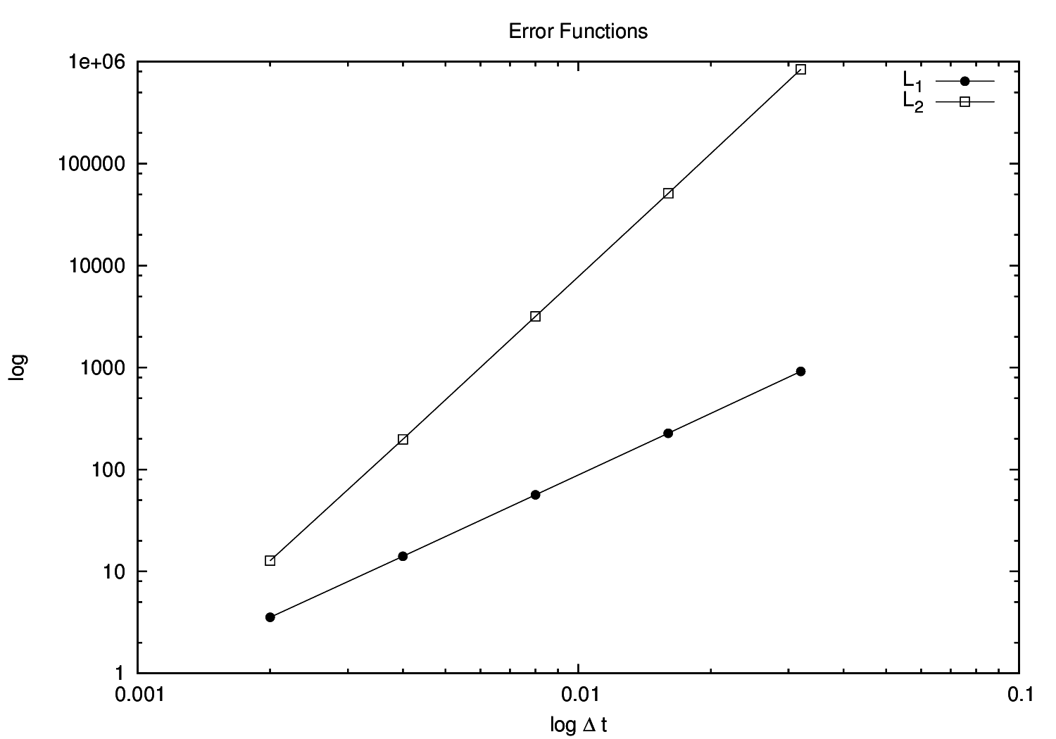
There are two important points that need to be addressed in a numerical work: one is the convergence of solutions and the other is the evolution of conserved quantities. Numerical solutions must also evolve on the constraint surface and they must preserve the conserved quantities. This ensures that they are evolving on the physical phase space. In figure 16 we show the convergence of the Hamiltonian constraint () and the field momentum evolution, which shows that is conserved. The quantities plotted in Figure 17 are the error functions
| (47) |
where the sub-indexes in the Hamiltonian constraint mean resolution (with ) and resolution (with ), such that . The method used to integrate the equations is a Runge-Kutta 4 (RK4), while the resolutions used for the convergence tests are . We can define the convergence order as
| (48) |
with any evolved function at resolution , with . The convergence factor for a RK4 must be and we get in our solutions , where denotes the average in time and taking the mean of different samples.
References
- [1] A. Ashtekar and P. Singh, “Loop Quantum Cosmology: A Status Report,” Class. Quant. Grav. 28 (2011) 213001 arXiv:1108.0893v2 [gr-qc]; I. Agullo and A. Corichi, “Loop Quantum Cosmology,” arXiv:1302.3833 [gr-qc].
- [2] A. Ashtekar, T. Pawlowski and P. Singh, “Quantum nature of the big bang: Improved dynamics,” Phys. Rev. D 74, 084003 (2006) arXiv:gr-qc/0607039.
- [3] A. Ashtekar, A. Corichi and P. Singh, “Robustness of key features of loop quantum cosmology,” Phys. Rev. D 77, 024046 (2008). arXiv:0710.3565 [gr-qc].
- [4] A. Corichi and E. Montoya, “Coherent semiclassical states for loop quantum cosmology,” Phys. Rev. D 84, 044021 (2011) arXiv:1105.5081 [gr-qc]; A. Corichi and E. Montoya, “On the Semiclassical Limit of Loop Quantum Cosmology,” Int. J. Mod. Phys. D 21, 1250076 (2012) arXiv:1105.2804 [gr-qc].
- [5] P. Diener, B. Gupt and P. Singh, “Numerical simulations of a loop quantum cosmos: robustness of the quantum bounce and the validity of effective dynamics,” Class. Quant. Grav. 31, 105015 (2014) arXiv:1402.6613 [gr-qc]; P. Diener, B. Gupt, M. Megevand and P. Singh, “Numerical evolution of squeezed and non-Gaussian states in loop quantum cosmology,” Class. Quant. Grav. 31, 165006 (2014) arXiv:1406.1486 [gr-qc].
- [6] L. Szulc, W. Kaminsk and J. Lewandowski, “Closed FRW model in Loop Quantum Cosmology,” Class. Quant. Grav. 24 (2007) 2621.A. Ashtekar, T. Pawlowski, P. Singh, and K. Vandersloot, “Loop quantum cosmology of k=1 FRW models,” Phys. Rev. D 75 (2007) 024035.
- [7] A. Corichi and A. Karami, “Loop quantum cosmology of k=1 FRW: A tale of two bounces”, Phys. Rev. D 84:044003 (2011), arXiv:1105.3724 [gr-qc].
- [8] A. Corichi and A. Karami, “Loop quantum cosmology of k=1 FLRW: Effects of inverse volume corrections,” Class. Quant. Grav. 31, 035008 (2014) arXiv:1307.7189 [gr-qc].
- [9] P. Singh and A. Toporensky, “Big Crunch Avoidance in k=1 Semiclassical Loop Quantum Cosmology,” Phys. Rev. D 69, 104008 (2004) arXiv:0312110 [gr-qc].
- [10] J. L. Dupuy, P. Singh, “Implications of quantum ambiguities in k=1 loop quantum cosmology: distinct quantum turnarounds and the super-Planckian regime,” arXiv:1608.07772 [gr-qc].
- [11] A. Corichi and P. Singh, “Is loop quantization in cosmology unique?,” Phys. Rev. D 78, 024034 (2008) arXiv:0805.0136 [gr-qc]; “A geometric perspective on singularity resolution and uniqueness in loop quantum cosmology,” Phys. Rev. D 80, 044024 (2009) arXiv:0905.4949 [gr-qc].
- [12] P. Singh and F. Vidotto, “Exotic singularities and spatially curved Loop Quantum Cosmology,” Phys. Rev. D 83, 064027 (2011) arXiv:1012.1307 [gr-qc].
- [13] P. Singh, “Curvature invariants, geodesics and the strength of singularities in Bianchi-I loop quantum cosmology”, Phys.Rev., D85, 104011,(2012).
- [14] P. Singh and E. Wilson-Ewing, “Quantization ambiguities and bounds on geometric scalars in anisotropic loop quantum cosmology”, Class. Quant. Grav. 31 035010 (2014) arXiv:1310.6728 [gr-qc].
- [15] P. Singh, “Is classical flat Kasner spacetime flat in quantum gravity?”, arXiv:1604.03828 [gr-qc]. Prepared for IJMPD special issue on Loop Quantum Cosmology.
- [16] A. Corichi and A. Karami, “Loop quantum cosmology of Bianchi IX: Inclusion of inverse triad corrections”, Int. J. Mod. Phys. D 25, 1642011 (2016). arXiv:1605.01383 [gr-qc].
- [17] M. Bojowald, G. Date and K. Vandersloot, “Homogeneous Loop Quantum Cosmology: The Role of the Spin Connection”, Class. Quant. Grav. 21, 1253 (2004); M. Bojowald and G. Date, “Quantum suppression of the generic chaotic behavior close to cosmological singularities”, Phys. Rev. Lett., 92, 071302, (2004); M. Bojowald, G. Date and G. M. Hossain, “The Bianchi IX model in Loop Quantum Cosmology”, Class. Quant. Grav. 21, 3541 (2004).
- [18] E. Wilson-Ewing, “Loop quantum cosmology of Bianchi type IX models,” Phys. Rev. D 82, 043508 (2010). arXiv:1005.5565 [gr-qc].
- [19] V. A. Belinskii, I. M. Khalatnikov, and E. M. Lifshitz, “Oscillatory approach to a singular point in relativistic cosmology”, Adv. Phys. 19, 525 (1970).
- [20] V. A. Belinskii, I. M. Khalatnikov, and E. M. Lifshitz, “A general solution of the Einstein equations with a time singularity”, Adv. Phys. 31, 639 (1982).
- [21] A. Ashtekar, A. Henderson and D. Sloan, “A Hamiltonian Formulation of the BKL Conjecture,” Phys. Rev. D 83, 084024 (2011) arXiv:1102.3474 [gr-qc].
- [22] K. C. Jacobs, “Spatially homogeneous and euclidean cosmological models with shear,” Astrophys. J. 153 (1968) 661.
- [23] J. Wainwright, G. F. R. Ellis, Dynamical Systems in Cosmology, Cambridge University Press (1997).
- [24] C. W. Misner, “Quantum Cosmology,” Phys. Rev. 186, 1319-1327 (1969); C. W. Misner, “Mixmaster Universe,” Phys. Rev. Lett. 22, Issue 20, 1071-1074 (1969).
- [25] D. W. Chiou and K. Vandersloot, “The behavior of non-linear anisotropies in bouncing Bianchi I models of loop quantum cosmology,” Phys. Rev. D 76, 084015 (2007) arXiv:0707.2548 [gr-qc]; D. W. Chiou, “Effective Dynamics, Big Bounces and Scaling Symmetry in Bianchi Type I Loop Quantum Cosmology,” Phys. Rev. D 76, 124037 (2007). arXiv:0710.0416 [gr-qc].
- [26] A. Ashtekar and E. Wilson-Ewing, “Loop quantum cosmology of Bianchi I models,” Phys. Rev. D79, 083535 (2009). arXiv:0903.3397 [gr-qc].
- [27] A. Corichi, A. Karami and E. Montoya, “Loop Quantum Cosmology of Bianchi IX: Qualitative effective dynamics”, unpublished, (2015).
- [28] A. Corichi, A. Karami and E. Montoya, “Loop Quantum Cosmology: Anisotropy and singularity resolution”, Springer Proc. Phys. 157 (2014) 469-477.
- [29] X. Lin and R. M. Wald, “Proof of the closed-universe-recollapse conjecture for diagonal Bianchi type-IX cosmologies”, Phys. Rev. D 40, 3280-6 (1989), Phys. Rev. D 41, 2444-8 (1990).
- [30] A. Karami, Aspects of loop quantization in cosmological models, Ph.D. Dissertation, Universidad Michoacana de San Nicolás de Hidalgo, Mexico (2014).
- [31] A. Ashtekar and E. Wilson-Ewing, “Loop quantum cosmology of Bianchi I models,” Phys. Rev. D79, 083535 (2009). arXiv:0903.3397 [gr-qc].
- [32] A. Ashtekar and E. Wilson-Ewing, “Loop quantum cosmology of Bianchi type II models,” Phys. Rev. D 80, 123532 (2009). arXiv:0910.1278 [gr-qc].
- [33] A. Corichi and E. Montoya, “Effective Dynamics in Bianchi Type II Loop Quantum Cosmology”, Phys. Rev. D, 85, 104052, (2012). arXiv:1201.4853; A. Corichi and E. Montoya, “Qualitative effective dynamics in Bianchi II loop quantum cosmology,” AIP Conf. Proc. 1473, 113 (2011).
- [34] A. Ashtekar, T. Pawlowski and P. Singh, “Quantum Nature of the Big Bang,” Phys. Rev. Lett. 96 (2006) 141301, arXiv:gr-qc/0602086.
- [35] A. Ashtekar, T. Pawlowski and P. Singh, “Quantum Nature of the Big Bang: An Analytical and Numerical Investigation,” Phys. Rev. D 73 (2006) 124038. arXiv:gr-qc/0604013.
- [36] B. Gupt and P. Singh, “Quantum gravitational Kasner transitions in Bianchi-I spacetime”, Phys. Rev. D, 86, 024034, (2012). arXiv:1205.6763 [gr-qc].
- [37] B. Gupt and P. Singh, “Contrasting features of anisotropic loop quantum cosmologies: the role of spatial curvature”, Phys. Rev. D, 85, 044011, (2012). arXiv:1109.6636 [gr-qc];