Measuring the functional connectome ‘on-the-fly’ — towards a new control signal for fMRI-based brain-computer interfaces
Abstract
There has been an explosion of interest in functional Magnetic Resonance Imaging (MRI) during the past two decades. Naturally, this has been accompanied by many major advances in the understanding of the human connectome. These advances have served to pose novel challenges as well as open new avenues for research. One of the most promising and exciting of such avenues is the study of functional MRI in real-time. Such studies have recently gained momentum and have been applied in a wide variety of settings; ranging from training of healthy subjects to self-regulate neuronal activity to being suggested as potential treatments for clinical populations. To date, the vast majority of these studies have focused on a single region at a time. This is due in part to the many challenges faced when estimating dynamic functional connectivity networks in real-time. In this work we propose a novel methodology with which to accurately track changes in functional connectivity networks in real-time. We adapt the recently proposed SINGLE algorithm for estimating sparse and temporally homogeneous dynamic networks to be applicable in real-time. The proposed method is applied to motor task data from the Human Connectome Project as well as to real-time data obtained while exploring a virtual environment. We show that the algorithm is able to estimate significant task-related changes in network structure quickly enough to be useful in future brain-computer interface applications.
Acknowledgements
The authors wish to thank Dr. Gregory Scott for providing help with the programming and preparation of the virtual reality platform used in the final application.
Data were provided (in part) by the Human Connectome Project, WU-Minn Consortium (Principal Investigators: David Van Essen and Kamil Ugurbil; 1U54MH091657) funded by the 16 NIH Institutes and Centers that support the NIH Blueprint for Neuroscience Research; and by the McDonnell Center for Systems Neuroscience at Washington University
1 Introduction
The notion of mind-controlled technology has been fueled by rapid advances in brain imaging over the last century. Since their early beginnings in the 1970s (Vidal, 1973; Vidal, 1977), brain-computer interfaces (BCI) have evolved into “one of the fastest growing areas of scientific research” (Mak and Wolpaw, 2009). Formally, a BCI is a system that measures brain activity and uses it to replace, restore, enhance, supplement, or improve normal output channels of peripheral nerves and muscles (Wolpaw and Wolpaw, 2011). While initial BCI research sought to enable communication with locked-in patients, its motivations and aspirations have since grown to encompass a wide range of applications such as motor rehabilitation (Birbaumer and Cohen, 2007) and movement restoration for the paralyzed (Müller-Putz et al., 2005). Moreover, BCI serves not only to bypass the brain’s natural motor output, but it can also transform brain signals into sensory input that can subsequently be used to modify cognitive state or behavior, a process referred to as neurofeedback (Ruiz et al., 2014).
Neurofeedback is a specific form of biofeedback whereby subjects are made aware of their brain activity in real-time. Such methods have been successfully employed to train the self-regulation of brain activity (Wolpaw et al., 2002; deCharms, 2008; Birbaumer et al., 2009; Weiskopf, 2012). Due to its inexpensive equipment and high temporal resolution, early neurofeedback research focused mainly on electroencephalography (EEG) as the preferred recording method. Yet, the lack of precise localization and the limited access to deep cortical and sub-cortical areas have limited future progress of EEG-based research. In contrast, functional magnetic resonance imaging (fMRI) has relatively high spatial resolution and whole brain coverage. Recent technical and methodological advances in acquisition and analysis have made real-time fMRI (rt-fMRI) a viable alternative when performing neurofeedback studies (Sitaram et al., 2011).
A recent literature review by Ruiz et al. (2014) highlighted that the vast majority of studies to-date have employed rt-fMRI for training healthy individuals to volitionally control BOLD activity in specific brain areas. Such region of interest (ROI) based neurofeedback training has been reported to dynamically reconfigure functional brain networks (Haller et al., 2013) and reinforce effective connectivity (Ruiz et al., 2013; Lee et al., 2012). However, while such ROI based studies have provided fundamental insights into functional architecture and cognition, they do no take into consideration the fact that complex cognitive processes are not limited to single brain regions but rather result from interactions between brain regions and between networks of regions (Sporns et al., 2004; Bressler and Menon, 2010; Koush et al., 2013; Ruiz et al., 2014). The next frontier for rt-fMRI studies corresponds to providing accurate and timely feedback to subjects based on entire functional connectivity networks as opposed to single ROIs, thereby providing a far richer description of a subjects’ brain state.
To date, there have been only a limited number of studies involving neurofeedback based on connectivity. One of the first studies to demonstrate self-regulation of functional connectivity networks was performed by Ruiz et al. (2014). Here a sliding window was used to provide subjects with a visual measure of functional connectivity between two ROIs. Zilverstand et al. (2014) performed an offline analysis showing that windowed correlations provide valuable information relating to task difficulty. Moreover, such measures of functional connectivity were shown to be more informative than univariate activation-based approaches. In a hypothesis-led study, Koush et al. (2013) presented a near real-time approach in which subjects learned to modulate the effective connectivity (assessed using dynamic causal modeling) between two pairs of ROIs.
These studies suggest that rt-fMRI connectivity is a useful tool for neurofeedback. However, such an endeavor presents considerable methodological challenges. Firstly, due to the nature of neurofeedback the resulting time series are expected to be non-stationary. The accurate estimation of non-stationary functional connectivity networks in an offline setting is a difficult problem in its own right and has recently received considerable attention (Bassett et al., 2011; Allen et al., 2012; Cribben et al., 2012; Monti et al., 2014; Davison et al., 2015). In this work we look to address this issue by extending recently proposed methods from the offline domain to the real-time domain. Second, due to potentially rapid changes that may occur in a subjects’ functional connectivity the proposed method must be both computationally efficient as well as highly adaptive to change. In order to satisfy the latter, the proposed method must be capable of accurately estimating functional connectivity networks using only a reduced (and adequately re-weighted) subset of current and past BOLD measurements.
To address these challenges, we first propose the use of exponentially weighted moving average (EWMA) models as well as more general adaptive forgetting techniques. This decision is motivated by the superior statistical properties of such approaches (Lindquist et al., 2014) as well as the need to ensure that the proposed methods are as adaptive as possible. We then extend the recently proposed Smooth Incremental Graphical Lasso Estimation (SINGLE) algorithm (Monti et al., 2014). Here functional relationships between pairs of nodes are estimated using partial correlations as opposed to Pearson’s correlation. Partial correlations are employed as they estimates pairwise correlations between nodes once the effects of all other nodes have been removed and have been shown to be better suited to detecting changes in network structure (Smith et al., 2011; Marrelec et al., 2009). We are able to re-cast the estimation of a new functional connectivity network as a convex optimization problem which can be quickly and efficiently solved in real-time.
The remainder of this manuscript is organized as follows: in Section 2 we introduce and describe the proposed method. In Section 3 we demonstrate the capabilities of the proposed method via a series of simulations. Finally, in Sections 4 and 5 we present two applications of the proposed algorithm. The first corresponds to a proof-of-concept study involving task-based data from the Human Connectome Project (Elam and Van Essen, 2014; Van Essen et al., 2012). While this data is not implicitly real-time, it may be treated as such to demonstrate the capabilities of the proposed method. The second application involves real-time fMRI data obtained from a single individual exploring a virtual environment.
2 Methods
We assume we have access to a stream of multivariate fMRI measurements across nodes where each node represents a region of interest (ROI). We write to denote the BOLD measurements at the time point across ROIs; thus corresponds to the BOLD measurement of the th node at time . In this work we are interested in sequentially using all observations up to and including to recursively learn the underlying functional connectivity networks. At time it is assumed we receive a new observation , which we use to update our network estimates accordingly. Throughout the remainder of this manuscript it is assumed that each follows a multivariate Gaussian distribution, , where both the mean and covariance structure are assumed to vary over time.
The functional connectivity network at time can be estimated by learning the corresponding precision (inverse covariance) matrices, . Such approaches have been employed extensively in neuroimaging applications (Varoquaux et al., 2010; Smith et al., 2011; Ryali et al., 2012) and have also recently been proposed to estimate time-varying estimates of functional connectivity networks (Allen et al., 2012; Cribben et al., 2012; Monti et al., 2014). Here encodes the partial correlations as well as the conditional independence structure at time . We then encode as a graph, , where the presence of an edge implies a non-zero entry in the corresponding entry of the precision matrix (Lauritzen, 1996).
Therefore, our aim is to estimate an increasing sequence of functional connectivity networks, where each captures the functional connectivity structure at the th observation. We wish for the proposed method to have the following properties:
- (a)
Real-time: first and foremost, networks should be estimated in real-time in order to provide subjects with feedback in a timely manner. This is of great importance as subjects require prompt feedback in order to successfully learn self-regulation.
- (b)
Adaptivity: we are particularly interested in the changes caused by the direct interaction with subjects while they are in the scanner. As such, it is crucial to be able to rapidly quantify changes in functional connectivity structure once these have occurred. The need for highly adaptive estimation methodologies is further exacerbated by the lagged nature of the hemodynamic response function, where changes in functional measurements typically occur six seconds after performing a task (LaConte et al., 2007).
- (c)
Accuracy: we also wish to accurately estimate network structure over time. This involves both the accurate estimation of network connectivity at each time point as well as the temporal evolution of pairwise relationships over time. That is to say, estimated networks should provide accurate representations of the true underling functional connectivity structure at any point in time as well as accurately describing how networks evolve over time.
Arguably the dominant approach used to obtain adaptive functional connectivity estimates involves the use of sliding windows (Hutchison et al., 2013) and this also holds true in the rt-fMRI setting (Gembris et al., 2000; Esposito et al., 2003; Ruiz et al., 2014; Zilverstand et al., 2014). Such methods are able to obtain adaptive functional connectivity estimates in real-time by only considering a fixed number of past observations, defined as the window. Using only the observations within the predefined window, a local (i.e., adaptive) estimate of functional connectivity is obtained. A natural extension of sliding windows are exponentially weighted moving average (EWMA) models, where observations are downweighted based on their chronological proximity — thereby giving more recent observations greater importance (Hunter, 1986). In such models, information from past observations is discarded at a constant rate determined by a fixed forgetting factor. Furthermore, adaptive forgetting methods can be seen as a generalization of EWMA models where the rate at which previous information is discarded is allowed to vary depending on the nature of the data (Haykin, 2008). This allows such algorithms to actively reduce the rate at which past information is discarded while networks remain relatively stable — resulting in more reliable network estimation — while also adapting rapidly to changes by increasing the rate at which past information is discarded in the presence of changes. These three methods, as well as their relationship, are discussed in detail in Section 2.1.
In order to ensure estimated networks provide an accurate representation of true functional connectivity networks we encourage two properties in estimated functional connectivity networks, . The first is sparsity; while functional connectivity networks are theorized to have evolved to achieve high efficiency of information transfer at a low connection cost (Bullmore and Sporns, 2009), the main motivation behind the introduction of sparsity here is statistical. Formally, the introduction of sparsity ensures the estimation problem remains feasible when the number of relevant observations falls below the number of parameters to estimate (Michel et al., 2011; Ryali et al., 2012). In the presence of rapid changes the number of relevant observations falls drastically. In such a scenario, sparse methods are able to guarantee the accurate estimation of functional connectivity networks without compromising the adaptivity of the proposed method. The second property we wish to encourage is temporal homogeneity; from a neurofeedback perspective we expect changes in functional connectivity structure to occur predominantly when paradigm changes occur (e.g., a subject begins performing a different task). Thus we expect network structure to remain constant within a neighbourhood of any observation but to vary over a longer period of time. We therefore encourage sparse innovations in network structure over time, ensuring that a change in connectivity is only reported when strongly substantiated by evidence in the data. Finally, real-time performance is achieved by casting the estimation as a convex optimization problem which can be efficiently solved.
The task of estimating in real time can be broken into two independent steps. First, an updated estimate of the sample covariance, , is calculated. We propose two methods with which an adaptive and accurate estimate of can be obtained: EWMA models and adaptive forgetting. In a second step, the corresponding precision matrix, , is estimated given the sample covariance. This is achieved by extending the recently proposed Smooth Incremental Graphical Lasso Estimation (SINGLE) algorithm (Monti et al., 2014) from the offline domain to the real-time domain.
The remainder of this section is organized as follows: in Section 2.1 we describe how adaptive estimates of the sample covariance can be obtained in real-time via the use of EWMA models or adaptive forgetting techniques. In Section 2.2 we outline the optimization algorithm employed. Parameter selection is discussed in Section 2.3.
2.1 Real-time, adaptive covariance estimation
The estimation of functional connectivity networks is fundamentally a statistical challenge (Friston, 1994) which is often studied by quantifying the pairwise correlations across various ROIs. Such approaches correspond directly to estimating and studying the covariance structure. When the functional time series is assumed to be stationary, this coincides with studying the sample covariance matrix for the entire dataset. However, in the case of rt-fMRI studies we are faced with data that is inherently non-stationary. Moreover, we have the additional constraint that data arrives sequentially over time, implying that information from new observations must be efficiently incorporated to update network estimates.
Addressing the non-stationary nature of the data is a challenging problem, even in the offline setting. Approaches such as change-point detection have been proposed (Robinson et al., 2010; Cribben et al., 2012), however the most widespread methodology involves the use of sliding windows or generalizations thereof. The advantage of such methods is that they are conceptually simple and can be easily extended to the real-time scenario as we describe below. A sliding window may be used to obtain a local estimate of the sample covariance, , at time as follows:
| (1) |
where is the mean of all observations falling within the sliding window and parameter is the length of the sliding window. It follows that determines the period of time over which previous observations are considered and will directly affect the adaptivity of the proposed algorithm.
A natural extension of sliding windows is the use of an exponentially weighted moving averages (EWMA), first introduced by Roberts (1959). Here observations are re-weighted according to their chronological proximity. The rate at which past information is discarded is determined by a fixed forgetting factor, . In this way, EWMA models are able to give greater importance to more recent observations thus increasing the adaptivity of the resulting algorithm. Moreover, as described in Lindquist et al. (2014), these methods enjoy superior statistical properties when compared to sliding window algorithms. EWMA models thereby provide a conceptually simple and robust method with which to handle a wide range of non-stationary processes. They are also particularly well suited to the real-time setting as we discuss below.
For a given forgetting factor, , the estimated mean at time can be recursively defined as:
| (2) |
where is a normalizing constant which is calculated as:
| (3) |
The sample covariance at time is subsequently defined as11 1 We note that equations (4) and (5) are equivalent to estimating the sample covariance in the more intuitive manner , however we choose to follow this parameterization in order to simplify future discussion.:
| (4) | ||||
| (5) |
From equations (2) and (4) we note that past observations gradually receive less importance. This is a contrast to sliding windows, where all observations receive equal weighting. It follows that the choice of parameter determines the rate at which information from previous observations is discarded and is directly related to the adaptivity of the proposed method. This can be seen by considering the extreme cases where and . Here we have that and consequently that and correspond to the sample mean and covariance estimated in an offline setting (using all observations up to time ). As a result equal importance is given to all observations, leading to reduced adaptivity to changes. As the value of is reduced, greater importance is given to more recent observations resulting in an increasingly adaptive estimate. Of course, as the value of decreases the estimated mean and covariance become increasing susceptible to outliers and noise. The choice of therefore constitutes a trade-off between adaptivity and stability.
Much like the length of the sliding window, , the choice of essentially determines the effective sample size used to estimate both and . Therefore the same logic applies when choosing both and : the value must be sufficiently large so as to allow robust estimation of the sample covariance without becoming too large (Sakoglu et al., 2010). This is discussed further in Section 2.3.
We further note that equations (3) - (5) make it clear how an real-time implementation of such methods would work. In practice only the most recent estimates of and would be stored together with from which new updates can efficiently be calculated.
2.1.1 Adaptive Forgetting
The use of both a sliding window or an EWMA model requires the specification of a fixed window length, , or forgetting factor, . The choice of these parameters makes implicit assumptions relating to the dynamics of the available data. It follows that large choices of and reflect an assumption that the data is close to being stationary. In such a scenario, large choices of and allow for accurate estimation of sample covariance matrices by adequately leveraging information across a wide range of observations. By the same token, smaller choices of and correspond to an assumption that the statistical properties of the data are changing at a faster rate.
However, it is important to note that for any non-stationary data the optimal choice of these parameters may depend on the location within the dataset. By this we mean that in the proximity to a change-point it would clearly be desirable to have smaller choice of and ; thereby reducing the influence of old, irrelevant observations. Whereas within a locally stationary region we wish to have a larger choices of and in order to effectively learn from a wide range of pertinent observations. This concept is demonstrated pictorially in the top panel of Figure [1].
Bottom: An illustration of how an ideal adaptive forgetting factor would behave; decreasing directly after a change occurs and quickly recovering thereafter.
In the case of real-time fMRI and neurofeedback we inherently expect the statistical properties of a subject’s functional connectivity networks to vary depending on both the task at hand as well as the neurofeedback. Therefore, the choice of a fixed window length, , or forgetting factor, , may be inappropriate.
In order to address this issue we propose the use of an adaptive forgetting methodology (Haykin, 2008). This corresponds to a selection of methods where the magnitude of the forgetting factor is adjusted directly from the data in real-time. As a result, the value of the forgetting factor has a direct dependence on the time index, . To make this relationship explicit we write to denote the adaptive forgetting factor at time . The bottom panel of Figure [1] provides an illustration of desirable behaviour for an adaptive forgetting factor. We note that immediately after a change occurs the forgetting factor drops. This helps discard past information which is no longer relevant and gives additional weighting to new observations. Moreover, it is also important to note that in the presence of piece-wise stationarity data the value of the adaptive forgetting factor increases, allowing for a larger number of observations to be leveraged and yielding more accurate and stable estimates.
Moreover, the use of adaptive forgetting also provides an additional monitoring mechanism. By considering the estimated value of the forgetting factor at any given point in time we can gain an understanding as to the current degree of non-stationarity in the data (Anagnostopoulos et al., 2012). This follows from the fact that the estimated forgetting factor quantifies the influence of recent observations on the sample mean and covariance. Thus it follows that large values of are indicative of piece-wise stationarity whereas small values of provide evidence for changes in the network structure.
In order to effectively learn the forgetting factor in real-time we require a data-driven approach. One popular solution is to empirically measure performance of current estimates by calculating the likelihood of incoming observations. In this way we are able to measure the performance of an estimated mean, , and sample covariance, , when provided with unseen data; thereby providing the basis on which to update our choice of forgetting factor. Under the assumption that all observations follow a multivariate Gaussian distribution, this likelihood of a new observation is:
| (6) |
While it would be possible to maximize using a cross-validation framework in an offline setting, such an approach is challenging in a real-time setting. This is because cross-validation approaches typically consider general performance over many subsets of past observations; therefore incurring a high computational cost. Moreover due to the highly autocorrelated nature of fMRI time series, splitting past observations into subsets is itself non-trivial. Here we build on the work of Anagnostopoulos et al. (2012) and employ adaptive forgetting methods to maximize this quantity in a computationally efficient manner. This is achieved by approximating the derivative of with respect to . This derivative can subsequently be used to update in a stochastic gradient ascent framework (Bottou, 2004).
From equations (2), (4) and (5) we can see the direct dependence of estimates and on a fixed forgetting factor . This suggests that the likelihood is itself a function of the forgetting factor, allowing us to calculate its derivative with respect to as follows:
| (7) | ||||
| (8) |
where have written to denote the derivative of with respect to (i.e., ). Full details are provided in Appendix A.
Given the derivative, , we can subsequently update our choice of forgetting factor using gradient ascent:
| (9) |
where is a small step-size parameter. Equation (9) serves to highlight the strengths of adaptive forgetting; by calculating we are able to learn the direction along which maximizes the log-likelihood of unseen observations. It follows that if is positive, should be increased, while the converse is true if is negative. Moreover, in calculating we also learn a magnitude. This implies that all updates in equation (9) will be of a different order of magnitude. This is fundamental as it allows for rapid adjustments in the presence of abrupt changes.
2.2 Real-time network estimation
We now turn to the problem of estimating the precision matrix at time . In this section, we describe how we can adapt the SINGLE algorithm in such a manner that we can obtain an estimated precision matrix that is both sparse and temporally homogeneous in real time.
Given a sequence of estimated sample covariance matrices , the SINGLE algorithm is able to estimate corresponding precision matrices, , by solving the following convex optimization problem:
| (11) |
The first sum in equation (11) corresponds to a likelihood term while the remaining terms, parameterized by and respectively, enforce sparsity and temporal homogeneity constraints. Estimated precision matrices, , therefore balance a trade-off between adequately describing observed data and satisfying sparsity and temporal homogeneity constraints.
However, in the real-time setting, a new is constantly obtained implying that the dimension of the solution to equation (11) grows over time. It follows that iteratively re-solving equation (11) is both wasteful and computationally expensive. In particular, valuable computational resources will be spent estimating past networks which are no longer of interest. In order to address this issue the following objective function is proposed to estimate the functional connectivity network at time :
| (12) |
where corresponds to the estimate of the precision matrix at time and is assumed to be fixed. The proposed real-time SINGLE (rt-SINGLE) algorithm is thus able to accurately estimate by minimizing equation (12) — in doing so the proposed method must find a balance between goodness-of-fit and satisfying the conditions of sparsity and temporal homogeneity. The former is captured by the likelihood term:
| (13) |
and provides a measure of how precisely describes the current estimate of the sample covariance, . The latter two terms of the objective correspond to regularization penalty terms:
| (14) |
The first of these, parameterized by , encourages sparsity while the second, parameterized by , determines the extent of temporal homogeneity. By penalizing changes in functional connectivity networks, the second penalty encourages sparse innovations in edge structure over time. As a result, network changes are only reported when heavily substantiated by evidence in the data. It is also important to note that equations (13) and (14) serve to formalize the separable nature of our objective function; a property we use to our advantage in the optimization algorithm.
2.2.1 Optimization algorithm
In order to efficiently minimize the rt-SINGLE objective function we introduce further adjustments. Equations (12)-(14) clearly expose the separable nature of the objective, which can be expressed as the sum of two sub-functions. It is precisely this property which is exploited in the original SINGLE algorithm by employing an Alternating Directions Method of Multipliers (ADMM) algorithm (Boyd et al., 2010). The ADMM is a form of augmented Lagrangian algorithm that is particularly well suited to addressing this class of separable and highly structured minimization problems. Formally, such an algorithm proceeds by iteratively minimizing each of the sub-functions together with an additional Lagrangian penalty term. As we demonstrate below, each of these minimization problems will either have a closed form solution or can be efficiently solved.
As in the SINGLE algorithm, we proceed by introducing an auxiliary variable . Here corresponds directly to and we require for convergence. Minimizing equation (12) can subsequently be cast as the following constrained optimization problem:
| (15) | ||||
| subject to | (16) |
We note that is now only involved in the likelihood component while is involved exclusively in the penalty component. Thus, by introducing we have decoupled the initial objective function — allowing us to take advantage of the individual structure associated with each term.
As in the SINGLE algorithm, we formulate the augmented Lagrangian corresponding to equations (15) and (16), which is defined as:
| (17) | ||||
where is the (scaled) Lagrange multiplier. Equation (17) corresponds to the Lagrangian together with an additional quadratic penalty term which serves to both increase the robustness of the proposed method (Bertsekas, 1982) as well as greatly simplify the resulting computations, as we describe below.
The proposed estimation algorithm works by iteratively minimizing equation (17) with respect to and while maintaining all other variables fixed. In this way, we are able to decouple the augmented Lagrangian and exploit the individual structure corresponding to each of these variables. Due to the iterative nature of the algorithm, in what follows we write to denote the estimate of at the th iteration. The same notation is used for both and . The algorithm is initialized with , . We note that the and update steps remain unchanged from the original offline algorithm. However, in the case of the update an adjustment is required due to the fact that past networks, , are treated as constants. Subsequently, is updated by solving:
| (18) |
where and are treated as constants. Here we note that equation (18) involves a series of one-dimensional problems as only element-wise operations are applied. This implies that we may solve an independent problem of the following form for each entry in :
| (19) |
where we write to denote the entry for any square matrix . Thus each element of can be updated by solving a one-dimensional convex problem. While there is no closed form solution, we may employ efficient line search algorithms (Boyd and Vandenberghe, 2004; Nocedal and Wright, 2006). Due to the symmetric nature of it follows that only of such problems must be solved.
2.2.2 Burn-in period
It is common for real-time algorithms to incorporate a brief burn-in phase a when they are initialized. This involves collecting the first observations and using these to collectively obtain the first estimate. Many times such an approach is motivated by the need to ensure sample statistics are well-defined, however due to the presence of regularization the proposed method does not require a burn-in per se. That said the use of a burn-in phase can improve initial network estimates and thereby result in improved network estimation overall. As a result, the first observations are collected and used to estimate the corresponding precision matrices by directly applying the offline SINGLE algorithm. This involves solving equation (11). From then onward, new estimates of the precision matrix are obtained as described previously.
2.3 Parameter tuning
Parameter estimation is challenging in the real-time setting. Approaches such as cross-validation, which are inherently difficult to implement due to the non-stationarity of the data, are further hampered by the limited computational resources. As an alternative, information theoretic approaches such as minimizing the AIC or BIC may be taken but these too may incur a high computational burden. In this section we discuss the three parameters required in the proposed method and provide a clear interpretation as well as a general overview on how each should be set.
The use of a sliding window or EWMA model implies an assumption about the non-stationarity of the data. Specifically, the underlying assumption behind such approaches is one of local, as opposed to global, stationarity. That is to say, we expect network structure to remain constant within a neighbourhood or any observation but to vary over a larger period of time. In choosing window length, , or the fixed forgetting factor, , we are inherently quantifying the size of this neighbourhood — a small value of or implies a small neighbourhood and is indicative of a system that varies quickly, while larger values imply slower, more gradual changes.
Defined in equation (3), provides an estimate for the effective sample size. That is, is indicative of the number of observations used in the calculation of the mean and sample covariance respectively. We note that as becomes large we have:
| (20) |
This allows us to directly quantify the effect of on the number of observations employed in each calculation. Furthermore, equation (20) also provides a clear relationship between the choice of window length and forgetting factor .
In practice, it is possible to choose the window length, , or forgetting factor, based on prior belief regarding the degree of non-stationarity in the data or using a maximum likelihood framework (Lindquist et al., 2007; Lindquist et al., 2014). A more elegant solution is provided via the use of adaptive forgetting methods. These methods designate the choice of to the data. As a result, only the stepsize parameter, , must be specified. Typical choices of range from to .
Parameters and enforce sparsity and temporal homogeneity respectively. The choice of these parameters affects the degrees of freedom of estimated networks, suggesting the use of information theoretic approaches such as AIC. However, in a real-time setting, choosing and in such a manner presents a computational burden. As a result, we propose two heuristics for choosing appropriate values of and respectively. One potential approach involves studying a previous scan of the subject in question. If this is available then the regularization parameters may be chosen by minimizing AIC over this scan. Alternatively, the burn-in phase may be used to choose adequate parameters. Such an approach would involve choosing and which minimized AIC over the burn in period. Moreover, it is worth noting that tuning and adaptively in a similar manner to the forgetting factor presents theoretical and computational challenges due to the non-differentiable nature of the regularization penalties.
3 Simulation study
3.1 Simulation settings
In this section we evaluate the performance of the rt-SINGLE algorithm through a series of simulation studies. In each simulation we produce simulated time series data giving rise to a number of connectivity patterns which reflect those reported in real fMRI data. The objective is then to measure whether our proposed algorithm is able recover the underlying patterns in real-time. We are primarily interested in studying the performance of the proposed methods in two ways; first we wish to study the quality of the estimated covariance matrices over time. That is to say, we study how accurately our sample covariances represent the true underlying covariance structure. Second, we are also interested in the correct estimation of the presence or absence of edges.
There are two main properties of fMRI data which we wish to recreate in the simulation study. The first is the high autocorrelation which is typically present in fMRI data (Poldrack et al., 2011). The second and main property we wish to recreate is the structure of the connectivity networks themselves. It is widely reported that brain networks have a small-world topology as well as highly connected hub nodes (Bullmore and Sporns, 2009) and we therefore look to enforce these properties in our simulated data.
Vector Autoregressive (VAR) processes are well suited to the task of producing autocorrelated multivariate time series as they are capable of encoding autocorrelations within components as well as cross correlations across components (Cribben et al., 2012). The focus of these simulations is to study the performance of the proposed method in the presence of non-stationary data. As a result the simulated datasets are only locally stationary. This is achieved by concatenating multiple VAR process which are simulated independently — this results in abrupt changes which are representative of the typical block structure of task based fMRI experiments.
Moreover, when simulating connectivity structures we study the performance of the proposed algorithm using two types of random graphs; scale-free random graphs obtained by using the preferential attachment model of Barabási and Albert (1999) and small-world random graphs obtained using the Watts and Strogatz (1998) model. The use of each of these types of networks is motivated by the fact that they are each known to each resemble different aspects of fMRI networks. Throughout each of the simulations, first the network architecture was simulated using either of the aforementioned methods. Then edge strength was uniformly sampled from . This introduced further variability into the simulated networks, increasing the difficulty of each task.
The simulations presented in this work look to quantify the ability of the rt-SINGLE algorithm to accurately estimate time-varying networks in real-time. In simulation I we study the quality of estimated covariance matrices over time. In simulations II and III we consider the overall performance of the proposed method by generating connectivity structures according to scale-free and small-world networks respectively. Finally, in Simulation IV we look to quantify the computational cost of the proposed method as the number of nodes, , increases. This simulation is fundamental in the neurofeedback setting as subjects must receive prompt and accurate feedback. Throughout this section we compare results for the rt-SINGLE algorithm where a fixed forgetting factor (corresponding to an EWMA model) is employed as well as adaptive forgetting techniques. Further, we also consider the performance of the offline SINGLE algorithm as a benchmark. Naturally we expect the rt-SINGLE algorithms to generally perform below its offline counterpart, however, the difference in performance will be indicative of how well the proposed methods work.
Throughout each of these simulations, the parameters for the offline SINGLE algorithm where determined as described in Monti et al. (2014). That is, the choice of kernel width was obtained by maximizing leave-one-out log-likelihood while the choice of regularization parameters where chosen by minimizing AIC. In the case of the real-time algorithms the parameters where chosen as follows. The fixed forgetting factor was chosen to be as this corresponded approximately to an effective sample size of twenty observations. While in the case of adaptive forgetting was chosen and a burn-in period of 15 observations was used. Regularization parameters where chosen to minimize AIC over the burn-in period.
3.2 Performance measures
As alluded to previously, we wish to evaluate the performance of the proposed method in two distinct ways. First, we wish to study the reliability with which we can track changes in covariance structure using either a fixed forgetting factor or an adaptive forgetting factor. In order to quantify the difference between the true covariance structure and our estimated covariance we consider the distance defined by the trace inner product:
| (21) |
It follows that if the estimated sample covariance, , is a good estimate of the true covariance, , we will have that . However, if is a poor estimate, the distance will be large. Moreover, since both and are positive definite we have that will always be positive.
Second, we wish to consider the estimated functional connectivity networks at each point in time. In this application we are particularly interested in correctly identifying the non-zero entries in estimated precision matrices, , at each . An edge is assumed to be present between the th and th nodes if . At the th observation we define the set of all reported edges as . We define the corresponding set of true edges as where we write to denote the true precision matrix at the th observation. Given and we consider a number of performance measures at each observation.
First we measure the precision, . This measures the percentage of reported edges which are actually present (i.e., true edges). Formally, the precision is given by:
Second we also calculate the recall, , formally defined as:
This measures the percentage of true edges which were reported by each algorithm. Ideally we would like to have both precision and recall as close to one as possible. Finally, the score, defined as
| (22) |
summarizes both the precision and recall by taking their harmonic mean. It follows that will lie on the interval with indicating perfect performance.
3.2.1 Simulation I — Covariance tracking
In this simulation we look to assess how accurately we are able to track changes in covariance structure via the use of fixed (i.e., EWMA models) and adaptive forgetting factors. As discussed previously, obtaining accurate estimates of the sample covariance in real-time is a fundamental problem both when studying functional connectivity networks in general and in particular for the proposed methods.
Here datasets were simulated as follows: each dataset consisted of five segments each of length 100 (i.e., overall duration of 500). The network structure within each segment were simulated according to either to either the Barabási and Albert (1999) preferential attachment model or using the Watts and Strogatz (1998) model. The use of each of these models was motivated by the fact that they are able to generate scale-free and small-world networks respectively; two classes of networks which are frequently encountered in the analysis of fMRI data (Eguiluz et al., 2005; Bassett and Bullmore, 2006; Sporns et al., 2004).
In this simulation the estimated sample covariances from the proposed methods were compared to the results when using a symmetric Gaussian kernel, as in the offline SINGLE algorithm. The choice of kernel width was determined by maximizing leave-one-out log-likelihood. In the case of the fixed forgetting factor, was chosen as this corresponded to an effective sample size of twenty observations. Finally, in the case of adaptive forgetting was chosen.
Figure [2] shows results when scale-free (left) and small-world (right) network structures are simulated. We note that the quality of the estimated covariances drops in the proximity of a change-point for all three algorithms. In the case of the offline SINGLE algorithm this drop is symmetric due to the symmetric nature of the Gaussian kernel employed. However, in the case of the real-time algorithms the drop is highly asymmetric and occurs directly after the change-point, as is to be expected. Due to the sudden change in covariance structure, these methods suffer immediately after abrupt changes in covariance structure, but are able to quickly recover. Moreover, from Figure [2] we note that the covariance tracking capabilities of the proposed methods are not adversely affected by the choice of underling network structure.
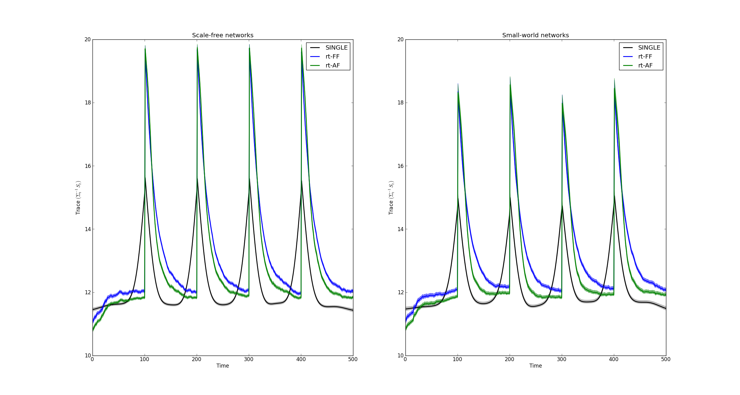
Left: Covariance tracking results when underling network structure is simulated according to the scale-free preferential attachment model of (Barabási and Albert, 1999). A change occurred every 100 observations. We note that the symmetric Gaussian kernel employed for the offline SINGLE algorithm outperforms the online algorithms as expected. However, when the covariance structure remains piece-stationary for extended periods of time the online algorithms are able to outperform their offline counterparts.
Right: Covariance tracking results when the underlying network structure was simulated using small-world random networks according to the model of Watts and Strogatz (1998).
3.2.2 Simulation II — Scale-free networks
In this simulation we look to obtain a general comparison between the rt-SINGLE algorithm and its offline counterpart. We simulated datasets with the following structure: each dataset consisted of five segments each of length 100 (i.e., overall duration of 500). The network structure within each segment was independently simulated according to the Barabási and Albert (1999) preferential attachment model. The motivation behind the use of the Barabási and Albert (1999) model is based on evidence that brain networks are scale-free, implying that the degree distribution follows a power law. This implies the presence of a reduced number of hub nodes which have access to many other regions, while the remaining majority of nodes have a small number of edges (Eguiluz et al., 2005).
In this simulation the entire dataset was simulated apriori. In the case of the rt-SINGLE algorithms, one observation was provided at time, thereby treating the dataset as if it was a stream arriving in real-time. The offline SINGLE algorithm was provided with the entire dataset and this was treated as an offline task.
In the left panel of Figure [3] we see the average scores for each of the real-time algorithms as well as the offline algorithm over 100 simulations. We note that all three algorithms experience a drop in -score in the proximity of change-points. The offline SINGLE algorithm is based on a symmetric Gaussian kernel, as a result, we note that there it has a symmetric drop in performance in the vicinity of a change-point before quickly recovering. Alternatively, the drop in performance of the rt-SINGLE algorithms is asymmetric. This is due to the real-time nature of these algorithms. Moreover, we note that while the rt-SINGLE algorithm performs worse than its offline counterpart directly after change-points, it is able to quickly recover to the level of the offline SINGLE algorithm. Specifically, in the case where adaptive forgetting is used, the real-time algorithm is able to outperform its offline counterpart in sections where the data remains piece-wise stationary for long periods of time. This is because it is able to increase the value of the adaptive forgetting factor accordingly. This allows the algorithm to exploit a larger pool of relevant information compared to its offline counterpart. This is demonstrated on the right panel of Figure [3] where the mean value of the adaptive forgetting factor is plotted. We see there is a drop directly after changes occur; this allows the algorithm to quickly forget past information which is no longer relevant. We also note that the estimate value of the forgetting factor increases quickly after changes occur.
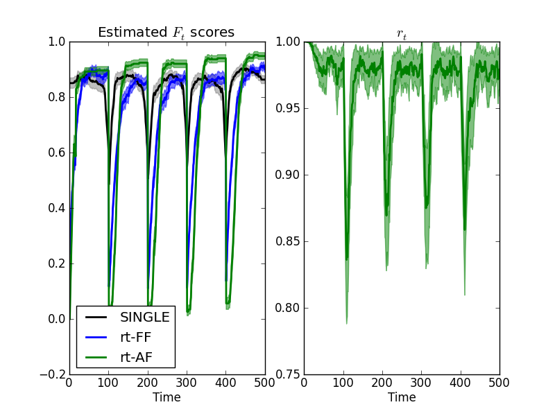
Right: mean values for the estimated adaptive forgetting factor, , over time. We note there is a sudden drop directly after changes occurs allowing the algorithm to adequately discard irrelevant information.
3.2.3 Simulation III — Small-world networks
While in Simulation II scale-free networks were studied, it has been reported that brain networks follow a small-world topology (Bassett and Bullmore, 2006). Such networks are characterized by their high clustering coefficients which has been reported in both anatomical as well as functional brain networks (Sporns et al., 2004).
The Watts and Strogatz (1998) model works as follows: starting with a regular lattice, the model is parameterized by which quantifies the probability of randomly rewiring an edge. It follows that setting results in a regular lattice, while setting results in an Erdős-Rényi (i.e., completely random) network structure. Throughout this simulation we set as this yielded networks with sufficient variability but which still displayed the desired small-world properties.
As in Simulation II the entire dataset was simulated apriori. In the case of the rt-SINGLE algorithms, one observation was provided at a time, thereby treating the dataset as if it were arriving in real-time. In the case of the offline SINGLE algorithm, the algorithm was provided with the entire dataset.
In the left panel of Figure [4] we see the average scores for each of the real-time algorithms as well as the offline SINGLE algorithm over 100 simulations. Due to the increased complexity of small-world networks, we note that the performance drops compared to scale-free networks considered in Simulation II. We further note that the rate at which the real-time networks recover after a change-point is reduced. As with Simulation II, we note that both of the real-time algorithms are able to reach the same level of performance as their offline counterpart if given sufficient time. Moreover, in the case where adaptive forgetting is employed we once again find that the performance of the real-time algorithm exceeds that of the offline algorithm when the data is remains piece-wise stationary for a sufficiently long period of time. In the right panel of Figure [4] we see the estimated adaptive forgetting factor over each of the 100 simulations. Again, we see the drop in the value of the forgetting factor directly after change-points; allowing past information to be efficiently discarded.
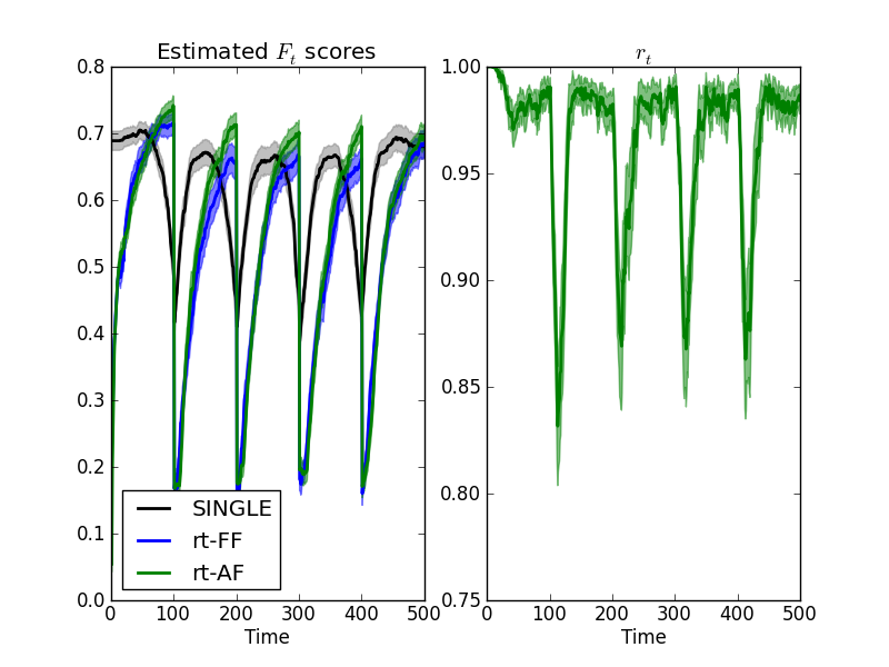
Right: mean values for the estimated adaptive forgetting factor, , over time. We note there is a sudden drop directly after changes occurs allowing the algorithm to adequately discard irrelevant information.
3.2.4 Simulation IV — Computational cost
A fundamental aspect of real-time algorithms is that they must be computationally efficient in order to be able to update parameter estimates in the limited time provided. The main computational cost of the rt-SINGLE algorithm is related to the eigendecomposition of the update, which has a complexity of (Monti et al., 2014).
In this simulation we look to empirically study the computational cost. In this manner, we are able to provide a rough guide as to the number of ROIs which can be employed in a real-time neurofeedback study while still reporting network estimates at every point in time. This was achieved by measuring the mean running time of each update iteration of the rt-SINGLE algorithm for various numbers of ROIs, .
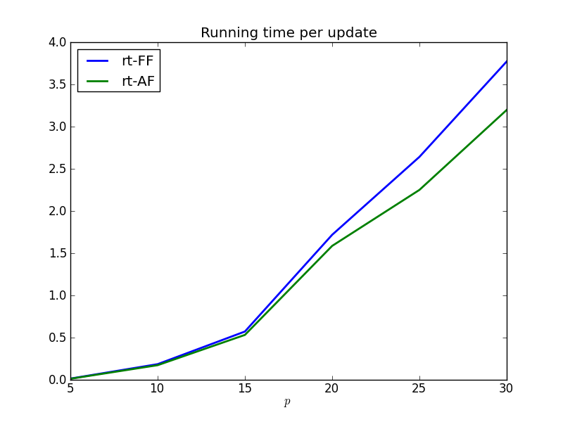
Here each dataset was simulated as in Simulation II; that is the underlying correlation was randomly generated according to a small-world network. However, here we choose to only simulate three segments, each of length 50, resulting in a dataset consisting of 150 observations. For increasing values of , the time taken to estimate a new precision matrix was calculated. Figure [5] shows the mean running time for the rt-SINGLE algorithm where either a fixed forgetting factor (i.e., an EWMA model) or adaptive forgetting was used. We note that the difference in computational cost between each of the algorithms is virtually indistinguishable.
Finally we note that for nodes, it is possible to estimate functional connectivity networks in under two seconds, making the proposed method practically feasible in many real-time studies. This simulation was run on a computer with an Intel Core i5 CPU at 2.8 GHz.
4 Application: HCP motor-task fMRI data
In this section we present the first of our applications. Here a motor-task dataset from the Human Connectome Project (Elam and Van Essen, 2014; Van Essen et al., 2012) is studied. While this dataset is not acquired and analyzed in real-time, it may be treated as such by only considering one observation at a time. This allows us to benchmark the rt-SINGLE algorithm to its offline counterpart using fMRI data as opposed to simulated examples, as we have done in Section 3.
4.1 Motor-task data
Twenty of the 500 available task-based fMRI datasets provided by the Human Connectome Project were selected at random. Here subjects were asked to perform a simple motor task adapted from those developed by Buckner et al. (2011) and Yeo et al. (2011). This involved the presentation of visual cues asking subjects to either tap their fingers (left or right), squeeze their toes (left or right) or move their tongue. Each movement type was blocked, lasting 12 seconds, and was preceded by a three second visual cue. In addition there were three 15 second fixation blocks per run22 2 for further details please see http://www.humanconnectome.org/documentation/Q1/task-fMRI-protocol-details.html.
While this data is not intrinsically real-time — in that the preprocessing was conducted after data acquisition — it is included as a proof-of-concept study. The data was preprocessed offline as the focus lies on the comparison between the real-time and offline network estimation approaches rather than different preprocessing pipelines. Preprocessing involved regression of Friston’s 24 motion parameters and high-pass filtering using a cut-off frequency of Hz.
Eleven bilateral cortical ROIs were defined based on the Desikan-Killiany atlas (Desikan et al., 2006) covering occipital, parietal and temporal lobe (see Table 1). The extracted time courses from these regions were subsequently used for the analysis. By treating the extracted time course data as if it was arriving in real-time (i.e., considering one observation at a time) we can compare the results of the proposed real-time method to offline algorithms while using the same underlying preprocessed data.
| Name | Right hem. | Left hem. | |||||
|---|---|---|---|---|---|---|---|
| Lateral Occipital | 31 | -84 | 1 | -29 | -87 | 1 | |
| Inferior Parietal | 43 | -62 | 30 | -39 | -68 | 30 | |
| Superior Parietal | 22 | -62 | 48 | -21 | -64 | 47 | |
| Precuneus | 11 | -56 | 37 | -10 | -57 | 37 | |
| Fusiform | 34 | -39 | -20 | -34 | -43 | -19 | |
| Lingual | 15 | -66 | -3 | -14 | -67 | -3 | |
| Inferior Temporal | 49 | -26 | -25 | -49 | -31 | -23 | |
| Middle Temporal | 57 | -22 | -14 | -56 | -27 | -12 | |
| Precentral | 39 | -8 | 43 | -38 | -9 | 43 | |
| Postcentral | 42 | -21 | 44 | -42 | -23 | 44 | |
| Paracentral | 9 | -26 | 58 | -8 | -28 | 59 | |
4.2 Results
Both the SINGLE as well as the rt-SINGLE algorithms where applied to the motor-task fMRI dataset. Our primary interest here is to report task-driven activations in functional connectivity. In this way, we are able to examine if the rt-SINGLE algorithm is capable of reporting changes in functional connectivity resulting from changes in motor task.
As a result, the functional relationships that were modulated by the motor task were studied; this corresponds to studying the edges in the estimated networks which are significantly correlated with task onset. This was achieved by first estimating time-varying functional connectivity networks using both the offline SINGLE algorithm as well as the proposed real-time algorithm. In the case of the SINGLE algorithm, parameters where chosen as described in Monti et al. (2014). This involved estimating the width of the Gaussian kernel via leave-one-out cross validation and estimating regularization parameters via minimizing AIC. In the case of the real-time algorithm, adaptive forgetting was employed with . The sparsity and temporal homogeneity parameters where set to the same values as the offline SINGLE algorithm as the focus here was to study differences induced by estimating networks in real-time as opposed to differences resulting from different parameterizations.
The correlation between estimated functional relationships (i.e., edges) and the task-evoked HRF function were estimated using Spearman’s rank correlation coefficient; a non-parametric measure of statistical dependence. The resulting -values (one for each edge) were then corrected for multiple comparisons via the Holm-Bonferroni method (Holm, 1979). This allowed us to obtain an activation network, summarizing which edges are statistically activated by task onset, for each algorithm.
Figure [6] shows task activation networks for both the SINGLE and rt-SINGLE algorithms. Here edges are only present if they were reported as being significantly correlated with task-evoked HRF function. Edge thickness is proportional to the estimated partial correlation between nodes. We note that there are visible similarities across each of the algorithms, indicating that the rt-SINGLE algorithm is accurately detecting task-modulated changes in functional connectivity. In particular there are clear similarities in functional connectivity patterns across the motorsensory regions.

These results serve as further evidence that the rt-SINGLE algorithm is capable of accurately detecting changes in real-time. Formally, the rt-SINGLE algorithm is able to detect patterns in functional connectivity associated with a motor task. It therefore follows that the estimated functional connectivity networks at each point in time could serve as input when looking to predict a subject’s brain state, as would be required in BCI applications.
5 Application: virtual world real-time fMRI data
While the HCP dataset introduced in Section 4 serves to demonstrate the reliability of the real-time network estimates, our proposed method was also tested using data that was processed and studied alongside data acquisition. In this proof-of-concept example study, we employed a more naturalistic and complex task that is similar to the type of situation likely to be used in closed-loop BCI systems. The study presented in this section involved a subject playing Minecraft, a popular virtual reality game, whilst in the scanner. The subject was instructed to explore the virtual world, during which time the background setting alternated between daylight and night. Here the objective was to measure if these changes could be reported by the proposed method in real-time.
5.1 Minecraft game
The subject was instructed to interactively explore a virtual game environment whilst lying in the MRI scanner. The game environment was created within the Minecraft framework (Mojang AB, Stockholm, Sweden). The experiment was repeated five times with each run consisting of the subject exploring the virtual world for 5 minutes (corresponding to 150 TRs). During this time, background brightness alternated between daylight and night in a 20 second blocked fashion. An example screenshot of changes seen by the subject is given in Figure [7]. The subject used button response boxes in both hands to move forward and turn left/right. The game was run on a separate machine which was connected to the real-time fMRI processing computer via a shared wireless network.

The study of the dataset is challenging for several reasons; first, correctly preprocessing and preparing the data in real-time is non-trivial and must be implemented efficiently in order to keep up with data acquisition. Moreover, further challenges arise due to the nature of the task performed. Formally, the task performed will activate visual, motor as well as higher level cognitive networks. Estimating such diverse networks with limited observations as well as limited computational resources therefore poses a large challenge.
5.2 Real-time fMRI setup
Whole brain coverage images were acquired in real-time by a Siemens Verio 3T scanner using an EPI sequence (T2*- of view mm, flip angle , time repetition (TR) / time echo (TE) = ms, 35 ascending slices). The reconstructed single EPI volume was exported from the MR scanner console to the real-time fMRI processing computer (Mac mini, 2.3 GHz Intel Quad Core i7, 16 GB RAM) via a shared network folder. Prior to the online run, a high-resolution gradient-echo T1-weighted structural anatomical volume (reference anatomical image, RAI with voxel size mm, flip angle , TR / TE = ms, 160 ascending slices, inversion time = 900 ms) and one EPI volume (reference functional image, RFI) needed to be acquired. The first step comprised the brain extraction of the RAI and RFI using BET (56), followed by an affine co-registration of the RFI to RAI and subsequent linear registration (12 DOF) to a standard brain atlas (MNI) using FLIRT (Jenkinson and Smith, 2001). The resulting transformation matrix was used to register the 11 anatomical ROIs (as described in Section 4.1 and Table 1) from MNI to the functional space of the respective subject. For online runs, incoming EPI images were converted from dicom to nifti file format and real-time motion correction was carried out using MCFLIRT (Jenkinson et al., 2002) with the previously obtained RFI acting as reference. ROI means of the anatomical maps for each TR were simultaneously extracted using a GLM approach and written into text file that was accessed by the rt-SINGLE algorithm. A burn-in period of 10 observations was employed. The first of the five runs was used to estimate sparsity and temporal homogeneity parameters by minimizing AIC. These parameters were subsequently used in the remaining four runs. Adaptive filtering was employed to estimate subject covariance matrices with tuning parameter . Preprocessing together with the rt-SINGLE optimization required under one second of computational time, making the proposed algorithm feasible within a neurofeedback setting.
5.3 Results
For each TR, updated ROI time courses were studied in real-time using the rt-SINGLE algorithm. Adaptive forgetting was employed with and regularization parameters where estimated by minimizing AIC over the subjects first run, these values where subsequently fixed throughout the remaining four runs.
As discussed previously, one of the additional benefits of adaptive forgetting is that further information can be gathered by studying the value of adaptive forgetting factor, , over time. Large values of are indicative of piece-wise stationary connectivity structures while small values serve to denote a period of instability. More importantly, sudden drops in the value of , as shown in Figures [3] and [4], can serve as a suggestion that a change has occurred and that the algorithm is quickly adapting. Figure [8] shows both the mean adaptive forgetting factors over all four runs as well as the adaptive forgetting factor estimated for a single run. The vertical dashed lines indicate when the background was changed from daylight to night or vice versa. We note that the forgetting factor quickly drops after most of these changes as we would expect. Moreover, there are no drops present during the first 20 seconds as this corresponds to the burn-in period employed.

The estimated networks can be used to study how functional connectivity is affected by changes related to daylight. By quantifying differences in the estimated functional connectivity networks we are able to report the edges that are indicative of daylight and night respectively. Figure [9] shows the edges that were significantly activated during daylight blocks. To determine the statistical significance of the reported changes a Wilcoxon rank-sum test was employed and the resulting -values where adjusted to correct for multiple comparisons using the Holm-Bonferroni method (Holm, 1979).
Figure [9] plots the statistically significant changes in functional connectivity modulated by changes in daylight settings. In particular, an increase in connectivity was detected during daylight blocks for visual-spatial and higher-level visual areas as well as higher-level visual and motorsensory areas. This is evident in Figure [9] which shows a clear hub of activated functional edges centered around the Lingual gyrus and the Fusiform gyrus regions; two regions typically associated with higher-order visual processing. It follows that information of this nature could be used to dictate feedback to subjects in real-time or as part of a BCI interface in future. Moreover, more advanced machine learning classifiers could be employed as described in LaConte et al. (2007).

6 Discussion
In this work we introduce a novel methodology with which to estimate dynamic functional connectivity networks in real-time. The strengths of the proposed method can be summarized as follows. First, the proposed method may leverage adaptive forgetting methods in order to obtain highly adaptive estimates of the sample covariance over time. Such methods designate that choice of the forgetting factor to the data, making them highly adaptive as well as flexible. The latter point is of particular importance in the rt-fMRI setting; since changes in functional connectivity may occur abruptly and at varying intervals the assumptions behind a fixed forgetting factor do not necessarily hold true. Second, by extending the recently proposed SINGLE algorithm we are able to accurately estimate functional connectivity networks based on precision matrices in real-time. The proposed method enforces constraints on both the sparsity as well as the temporal homogeneity of estimated functional connectivity networks. The former is required in order to ensure the estimation problem remains well-posed when the number of relevant observations drops, as is bound to occur when adaptive forgetting is employed. On the other hand, the temporal homogeneity constraint ensures changes in functional connectivity are only reported when heavily substantiated by evidence in the data. As a result, the rt-SINGLE algorithm is able to both obtain accurate estimates of functional connectivity networks at each point in time as well as accurately describe the evolution of networks over time.
The rt-SINGLE algorithm is closely related to sliding window methods which have been employed extensively in the real-time setting (Gembris et al., 2000; Esposito et al., 2003; Ruiz et al., 2014; Zilverstand et al., 2014). Extensions of sliding window methods, such as EWMA models, have been successfully applied to offline fMRI studies (Lindquist et al., 2007) and have been shown to be better suited to estimating dynamic functional connectivity (Lindquist et al., 2014). In this work EWMA models are considered alongside adaptive forgetting. The latter can be interpreted as a natural extension of EWMA models, where the rate at which past observations are discarded is learnt from the data. The proposed method is flexible and can be implemented using either a fixed forgetting factor (corresponding to an EWMA model) or using adaptive forgetting.
The proposed method requires the input of three parameters. The first of these parameters affects the manner in which sample covariance matrices are estimated. As noted previously, this can be achieved either using an EWMA model or via adaptive forgetting. If the former is used a fixed forgetting factor, , must be specified. As discussed in Section 2.3, the choice of can be interpreted as defining a weighted window. It therefore follows that the choice of must balance a trade-off between stability and adaptivity. A small choice of implies past observations are quickly discarded. While this will result in highly adaptive estimates, it may also result in network estimates that are dominated by noise. Conversely, a large value of will diminish the adaptive properties of the proposed method whilst producing more stable estimates. Alternatively, the use of adaptive forgetting requires the input of a stepsize parameter . This parameter governs the rate at which an adaptive forgetting factor, , varies and can be interpreted as the stepsize in a stochastic gradient descent scheme (Bottou, 2004). As such, it is typically suggested to set in the range of to . The final two parameters enforce sparsity and temporal homogeneity respectively. These parameters remain fixed throughout in a similar manner to the fixed forgetting factor and two heuristic approaches are proposed to tune these parameters. A future improvement for the proposed algorithm would involve adaptive regularization penalties. However, such approaches are computationally and theoretically challenging due to the non-differentiable nature of the penalty terms.
Several simulations are presented to examine the properties of the proposed method. These serve to demonstrate that the proposed method is capable of accurately estimating functional connectivity networks in real-time. Formally, we investigate three specific properties of the proposed method. First, in simulation I, we quantify how effectively the proposed method can track changes in covariance structure over time. Second, simulations II and III we study how accurately the rt-SINGLE algorithm can estimate functional connectivity networks. Finally, the computational cost of the proposed method is considered in simulation IV. This is fundamental in the case of real-time algorithms as estimated networks must be reported for each observation.
Two applications of the proposed method are provided. The first involves motor-task data from the HCP. While this data is not intrinsically real-time, it is included as a proof-of-concept study to validate the proposed method. The results demonstrate that the rt-SINGLE algorithm is able to accurately detect functional networks which are modulated by motor task. The second application corresponds to a more complex real-time study which is more closely related to the type of situation which may be employed in a closed-loop BCI system. This study required the subject to explore a virtual game environment while in the scanner. Throughout this time, the background brightness alternated between daylight and night in a block fashion. The changes in background brightness induced changes in functional connectivity that were subsequently reported, in real-time, by the proposed method. Specifically, the proposed method is able to detect a network of edges that was activated during daylight. In future, such information could be incorporated into a neurofeedback or BCI setting.
In conclusion, the rt-SINGLE algorithm provides a novel method for estimating functional connectivity networks in real-time. We present two applications demonstrating that the rt-SINGLE algorithm is capable of reporting changes in functional connectivity related to changes in task as well as external stimuli. In future, we look forward to incorporating the proposed method in a more extensive real-time neurofeedback study.
Appendix
A Full derivation of Adaptive filtering derivative
The results shown in this section are taken from Anagnostopoulos et al. (2012).
The log-likelihood for unseen observation, is given by
| (23) |
The approach taken here is to approximate the derivative of with respect to adaptive forgetting factor by calculating the exact derivative of with respect to a fixed forgetting factor . Then under the assumption that changes in occur sufficiently slowly, this will serve as a good approximation to the derivative of with respect to .
We begin by noting the following results from Petersen and Pedersen (2008):
| (24) | ||||
| (25) |
Moreover, we note that we do not need to explicitly invert . By noting that is a rank one update of we are able to directly obtain using the Sherman-Woodbury formula.
References
- Allen et al. [2012] E. Allen, E. Damaraju, S. Plis, E. Erhardt, T. Eichele, and V. Calhoun. Tracking whole-brain connectivity dynamics in the resting state. Cerebral cortex, page bhs352, 2012.
- Anagnostopoulos et al. [2012] C. Anagnostopoulos, D. Tasoulis, N. Adams, N. Pavlidis, and D. Hand. Online linear and quadratic discriminant analysis with adaptive forgetting for streaming classification. Statistical Analysis and Data Mining, 5(2):139–166, 2012.
- Barabási and Albert [1999] A. Barabási and R. Albert. Emergence of scaling in random networks. Science, 286(5439):509–512, 1999.
- Bassett and Bullmore [2006] D. Bassett and E. Bullmore. Small-world brain networks. The Neuroscientist, 12(6):512–523, 2006.
- Bassett et al. [2011] D. Bassett, N. Wymbs, M. Porter, P. Mucha, J. Carlson, and S. Grafton. Dynamic reconfiguration of human brain networks during learning. Proceedings of the National Academy of Sciences, 108(18):7641–7646, 2011.
- Bertsekas [1982] D. P. Bertsekas. Constrained Optimisation and Lagrange Multiplier Methods. Academic Press, 1982.
- Birbaumer and Cohen [2007] N. Birbaumer and L. Cohen. Brain-computer interfaces: communication and restoration of movement in paralysis. The Journal of physiology, 579(3):621–636, 2007.
- Birbaumer et al. [2009] N. Birbaumer, A. Ramos Murguialday, C. Weber, and P. Montoya. Neurofeedback and brain–computer interface: clinical applications. International Review of Neurobiology, 86:107–117, 2009.
- Bottou [2004] L. Bottou. Stochastic learning. In Advanced lectures on machine learning, pages 146–168. Springer, 2004.
- Boyd and Vandenberghe [2004] S. Boyd and L. Vandenberghe. Convex Optimization. Cambridge University Press, 2004.
- Boyd et al. [2010] S. Boyd, N. Parikh, E. Chu, B. Peleato, and J. Eckstein. Distributed Optimization and Statistical Learning via the Alternating Direction Method of Multipliers. Foundations and Trends in Machine Learning, 3(1):1–122, 2010.
- Bressler and Menon [2010] S. Bressler and V. Menon. Large-scale brain networks in cognition: emerging methods and principles. Trends in cognitive sciences, 14(6):277–290, 2010.
- Buckner et al. [2011] R. Buckner, F. Krienen, A. Castellanos, J. Diaz, and B.T. Yeo. The organization of the human cerebellum estimated by intrinsic functional connectivity. Journal of neurophysiology, 106(5):2322–2345, 2011.
- Bullmore and Sporns [2009] E. Bullmore and O. Sporns. Complex brain networks: graph theoretical analysis of structural and functional systems. Nature, 10:186–198, 2009.
- Cribben et al. [2012] I. Cribben, R. Haraldsdottir, Y. L. Atlas, T. D. Wager, and M. A Lindquist. Dynamic Connectivity Regression: Determining state-related changes in brain connectivity. NeuroImage, 61(4):907–920, 2012.
- Davison et al. [2015] E. Davison, K. Schlesinger, D. Bassett, M. Lynall, M. Miller, S. Grafton, and J. Carlson. Brain network adaptability across task states. PLoS computational biology, 11(1):e1004029, 2015.
- deCharms [2008] C. deCharms. Applications of real-time fMRI. Nature Reviews Neuroscience, 9(9):720–729, 2008.
- Desikan et al. [2006] R. Desikan, F. Ségonne, B. Fischl, B. Quinn, B. Dickerson, D. Blacker, R Buckner, A. Dale, R. Maguire, and B. Hyman. An automated labeling system for subdividing the human cerebral cortex on mri scans into gyral based regions of interest. Neuroimage, 31(3):968–980, 2006.
- Eguiluz et al. [2005] V. M. Eguiluz, D. R. Chialvo, G. A. Cecchi, M. Baliki, and A. V. Apkarian. Scale-free brain functional networks. Physical review letters, 94(1):018102, 2005.
- Elam and Van Essen [2014] J. Elam and D. Van Essen. Human Connectome Project. In Encyclopedia of Computational Neuroscience, pages 1–4. Springer, 2014.
- Esposito et al. [2003] F. Esposito, E. Seifritz, E. Formisano, R. Morrone, T. Scarabino, G. Tedeschi, S. Cirillo, R. Goebel, and F. Di Salle. Real-time independent component analysis of fmri time-series. Neuroimage, 20(4):2209–2224, 2003.
- Friston [1994] K. Friston. Functional and effective connectivity in neuroimaging: a synthesis. Human Brain Mapping, 2(1):56–78, 1994.
- Gembris et al. [2000] D. Gembris, J. Taylor, S. Schor, W. Frings, D. Suter, and S. Posse. Functional magnetic resonance imaging in real time (fire): Sliding-window correlation analysis and reference-vector optimization. Magnetic Resonance in Medicine, 43(2):259–268, 2000.
- Haller et al. [2013] S. Haller, R. Kopel, P. Jhooti, T. Haas, F. Scharnowski, K. Lovblad, K. Scheffler, and D. Van De Ville. Dynamic reconfiguration of human brain functional networks through neurofeedback. NeuroImage, 81:243–252, 2013.
- Haykin [2008] S. Haykin. Adaptive filter theory. Pearson, 2008.
- Holm [1979] S. Holm. A simple sequentially rejective multiple test procedure. Scandinavian journal of statistics, pages 65–70, 1979.
- Hunter [1986] J. S. Hunter. The exponentially weighted moving average. Journal of Quality Technology, 18(4):203–210, 1986.
- Hutchison et al. [2013] M. Hutchison, T. Womelsdorf, E. Allen, P. Bandettini, V. Calhoun, M. Corbetta, S. Della Penna, J. Duyn, G. Glover, J. Gonzalez-Castillo, et al. Dynamic functional connectivity: promise, issues, and interpretations. Neuroimage, 80:360–378, 2013.
- Jenkinson and Smith [2001] M. Jenkinson and S. Smith. A global optimisation method for robust affine registration of brain images. Medical image analysis, 5(2):143–156, 2001.
- Jenkinson et al. [2002] M. Jenkinson, P. Bannister, M. Brady, and S. Smith. Improved optimization for the robust and accurate linear registration and motion correction of brain images. Neuroimage, 17(2):825–841, 2002.
- Koush et al. [2013] Y. Koush, M. Rosa, F. Robineau, K. Heinen, S. Rieger, N. Weiskopf, P. Vuilleumier, D. Van De Ville, and F. Scharnowski. Connectivity-based neurofeedback: dynamic causal modeling for real-time fMRI. NeuroImage, 81:422–430, 2013.
- LaConte et al. [2007] S. LaConte, S. Peltier, and X. Hu. Real-time fMRI using brain-state classification. Human brain mapping, 28(10):1033–1044, 2007.
- Lauritzen [1996] S. Lauritzen. Graphical models. Oxford University Press, 1996.
- Lee et al. [2012] J. Lee, J. Kim, and S. Yoo. Real-time fMRI-based neurofeedback reinforces causality of attention networks. Neuroscience research, 72(4):347–354, 2012.
- Lindquist et al. [2007] M. Lindquist, C. Waugh, and T. Wager. Modeling state-related changes in fMRI activity using change-point theory. NeuroImage, 5(3):1125–1141, 2007.
- Lindquist et al. [2014] M. Lindquist, Y. Xu, M. Nebel, and B. Caffo. Evaluating dynamic bivariate correlations in resting-state fMRI: A comparison study and a new approach. NeuroImage, 2014.
- Mak and Wolpaw [2009] J. Mak and J. Wolpaw. Clinical applications of brain-computer interfaces: current state and future prospects. Biomedical Engineering, IEEE Reviews in, 2:187–199, 2009.
- Marrelec et al. [2009] G. Marrelec, J. Kim, J. Doyon, and B. Horwitz. Large-scale neural model validation of partial correlation analysis for effective connectivity investigation in functional MRI. Human brain mapping, 30(3):941–950, 2009.
- Michel et al. [2011] V. Michel, A. Gramfort, G. Varoquaux, E. Eger, and B. Thirion. Total variation regularization for fMRI-based prediction of behavior. Medical Imaging, IEEE Transactions on, 30(7):1328–1340, 2011.
- Monti et al. [2014] R. P. Monti, P. Hellyer, D. Sharp, R. Leech, C. Anagnostopoulos, and G. Montana. Estimating time-varying brain connectivity networks from functional MRI time series. NeuroImage, 103:427–443, 2014.
- Müller-Putz et al. [2005] G. Müller-Putz, R. Scherer, G. Pfurtscheller, and R. Rupp. EEG-based neuroprosthesis control: a step towards clinical practice. Neuroscience letters, 382(1):169–174, 2005.
- Nocedal and Wright [2006] J. Nocedal and S. J. Wright. Numerical Optimisation. Springer, 2006.
- Petersen and Pedersen [2008] K. Petersen and M. Pedersen. The matrix cookbook. Technical University of Denmark, pages 7–15, 2008.
- Poldrack et al. [2011] R. A. Poldrack, J. A. Mumford, and T. E. Nichols. Handbook of Functional MRI Data Analysis. Cambridge University Press, 2011.
- Roberts [1959] S. Roberts. Control chart tests based on geometric moving averages. Technometrics, 1(3):239–250, 1959.
- Robinson et al. [2010] L. Robinson, T. Wager, and M. Lindquist. Change point estimation in multi-subject fMRI studies. NeuroImage, 49(2):1581–1592, 2010.
- Ruiz et al. [2013] S. Ruiz, S. Lee, S. Soekadar, A. Caria, R. Veit, T. Kircher, N. Birbaumer, and R. Sitaram. Acquired self-control of insula cortex modulates emotion recognition and brain network connectivity in schizophrenia. Human Brain Mapping, 34(1):200–212, 2013.
- Ruiz et al. [2014] S. Ruiz, K. Buyukturkoglu, M. Rana, N. Birbaumer, and R. Sitaram. Real-time fMRI brain computer interfaces: self-regulation of single brain regions to networks. Biological psychology, 95:4–20, 2014.
- Ryali et al. [2012] S. Ryali, T. Chen, K. Supekar, and V. Menon. Estimation of functional connectivity in fmri data using stability selection-based sparse partial correlation with elastic net penalty. Neuroimage, 59(4):3852–3861, 2012.
- Sakoglu et al. [2010] U. Sakoglu, G. D. Pearlson, K. A. Kiehl, Y. M. Wang, A. M. Micheal, and V. D. Calhoun. A method for evaluating dynamic functional network connectivity and task modulation: application to Schizophrenia. Magnetic Resonance Materials in Physics, Biology and Medicine, 23:351–366, 2010.
- Sitaram et al. [2011] R. Sitaram, S. Lee, S. Ruiz, and N. Birbaumer. Real-time regulation and detection of brain states from fMRI signals. Neurofeedback and Neuromodulation Techniques and Applications, page 227, 2011.
- Smith et al. [2011] S. Smith, K. Miller, G. Salimi-Khorshidi, M. Webster, C. Beckmann, T. Nichols, J. Ramsey, and M. Woolrich. Network modelling methods for fMRI. Neuroimage, 54(2):875–891, 2011.
- Sporns et al. [2004] O. Sporns, D. R. Chialvo, M. Kaiser, and C. C. Hilgetag. Organization, development and function of complex brain networks. Trends in Cognitive Sciences, 8(9):418–425, 2004.
- Van Essen et al. [2012] D. Van Essen, K. Ugurbil, E. Auerbach, D. Barch, T. Behrens, R. Bucholz, A. Chang, L. Chen, M. Corbetta, and S. Curtiss. The Human Connectome Project: a data acquisition perspective. Neuroimage, 62(4):2222–2231, 2012.
- Varoquaux et al. [2010] G. Varoquaux, A. Gramfort, J. Poline, and B. Thirion. Brain covariance selection: better individual functional connectivity models using population prior. In Advances in Neural Information Processing Systems, pages 2334–2342, 2010.
- Vidal [1973] J. Vidal. Toward direct brain-computer communication. Annual review of Biophysics and Bioengineering, 2(1):157–180, 1973.
- Vidal [1977] J. Vidal. Real-time detection of brain events in EEG. Proceedings of the IEEE, 65(5):633–641, 1977.
- Watts and Strogatz [1998] D. J. Watts and S. H. Strogatz. Collective dynamics of small-world networks. Nature, 393(6684):440–442, 1998.
- Weiskopf [2012] N. Weiskopf. Real-time fMRI and its application to neurofeedback. Neuroimage, 62(2):682–692, 2012.
- Wolpaw and Wolpaw [2011] J. Wolpaw and E. Wolpaw. Brain-computer interfaces: principles and practice. Oxford University Press, 2011.
- Wolpaw et al. [2002] J. Wolpaw, N. Birbaumer, D. McFarland, G. Pfurtscheller, and T. Vaughan. Brain–computer interfaces for communication and control. Clinical neurophysiology, 113(6):767–791, 2002.
- Yeo et al. [2011] B.T. Yeo, F. Krienen, J. Sepulcre, M. Sabuncu, D. Lashkari, M. Hollinshead, J. Roffman, J. Smoller, L. Zöllei, and J. Polimeni. The organization of the human cerebral cortex estimated by intrinsic functional connectivity. Journal of neurophysiology, 106(3):1125–1165, 2011.
- Zilverstand et al. [2014] A. Zilverstand, B. Sorger, J. Zimmermann, A. Kaas, and R. Goebel. Windowed correlation: a suitable tool for providing dynamic fMRI-based functional connectivity neurofeedback on task difficulty. PloS one, 9(1):e85929, 2014.