Algorithms for Finding Copulas
Minimizing Convex Functions of
Sums
Abstract
We develop improved rearrangement algorithms to find the dependence structure that minimizes a convex function of the sum of dependent variables with given margins. We propose a new multivariate dependence measure, which can assess the convergence of the rearrangement algorithms and can be used as a stopping rule. We show how to apply these algorithms for example to finding the dependence among variables for which the marginal distributions and the distribution of the sum or the difference are known. As an example, we can find the dependence between two uniformly distributed variables that makes the distribution of the sum of two uniform variables indistinguishable from a normal distribution. Using MCMC techniques, we design an algorithm that converges to the global optimum.
Key-words: Multivariate risk measure, Block RA, Rearrangement algorithm, minimum variance, discrete optimization, MCMC, copula.
Algorithms for Finding Copulas
Minimizing Convex Functions of Sums
Introduction
For specified marginal distributions such as the uniform or the normal distribution, can we find a dependence structure or copula, which provides a specific distribution for the sum of variables? What if we were to require that the sum be constant? Questions like this have been addressed theoretically in the literature in a number of papers with the concept of complete mixability (Wang and Wang (2011), Puccetti and Wang (2015b), Wang and Wang (2016) to cite only a few), and computationally, with the rearrangement algorithm (RA) (Puccetti and Rüschendorf (2012), Embrechts, Puccetti, and Rüschendorf (2013)). The RA aims to minimize the expectation of a convex function of a sum of random variables (including the case of minimization of the variance of the sum as a special case).11 1 More details on the RA can be found at https://sites.google.com/site/rearrangementalgorithm/. This algorithm is fast and simple but may not converge to the global minimum. In particular, it does not depend on the convex function to minimize. Our main objective in this paper is to further this discussion by developing an improved version of this algorithm.
The minimization of convex functions of a sum of dependent random variables can be formulated using a matrix , and is linked to the problem of minimizing a convex function of the row sums over all permutations within the columns. It is a highly computationally complex problem, as even in the special case of columns, it has been shown to be NP-complete (Haus (2015)). It means that no algorithm will guarantee convergence to the optimum in polynomial time. Enumeration might be considered, but for reasonable sized matrices this is also not feasible. For a matrix, the number of essentially distinct matrices that can be obtained is the number of permutations of the columns other than the first, which is For example, for a small matrix this is obviously completely impossible by enumeration. Various versions of this problem have been treated in the literature, and algorithms proposed for special cases, but because the problem is NP complete (see Hsu (1984)), these algorithms do not converge to an optimal. For example Coffman and Yannakakis (1984) propose an algorithm designed to minimize the maximum of the row sums (the assembly line crew scheduling problem) and show that this algorithm converges to a solution less than 1.5 times the optimal. The NP complete nature of the problem indicates that the worst case performance of algorithms may be unsatisfactory, but it is still possible to develop algorithms, which normally find the optimum very quickly. We present Markov Chain algorithms here, which guarantee finding the global optimum in finite time, usually very rapidly.
There are many more applications for the Rearrangement Algorithm (RA) of Puccetti and Rüschendorf (2012). It has been used successfully in recent advances to the risk management field. Specifically, the RA is used to measure model risk on dependence, also called “dependence uncertainty,” and can help regulators to make decisions on which risk measure is most appropriate to compute capital requirements (see Embrechts, Puccetti, Rüschendorf, Wang, and Beleraj (2014)). It was successfully used to approximate VaR bounds on the sum of dependent risks with given marginal distributions by Embrechts, Puccetti, and Rüschendorf (2013) by applying the RA to the largest rows of the matrix such that all risks are comonotonic. Many more applications of this RA have been recently developed. Among others, Aas and Puccetti (2014) use the standard RA to compute capital requirements of DNB bank, Bernard, Rüschendorf, and Vanduffel (2016), Bernard, Rüschendorf, Vanduffel, and Yao (2016) to assess portfolios’ credit risk and Bernard and Vanduffel (2015) to incorporate partial information on dependence in the computation of bounds on capital requirements, Bernard, Jiang, and Wang (2014) to derive bounds on convex risk measures and quantify dependence uncertainty and Puccetti and Wang (2015a) to detect complete mixability. As we expect many more applications of such algorithms, it is important to develop efficient and accurate algorithms that converge to a minimum, a feature of our algorithms.
In this paper, we develop a novel application. We are able to find the dependence structure such that the sum of dependent variables has a prescribed distribution. We will refer to two distributions and as “close" if a large sample from one, say from , cannot be detected as not coming from with high probability using a standard test. We will use the Kolmogorov-Smirnov test and the Wasserstein distance test. This allows us, for example, to find two dependent Uniform[0,1] random variables such that is nearly 0 where is a normally distributed variable with mean and variance , in other words so that is nearly normal.
This toy example illustrates a potential use of the methodology to infer the dependence among variables that can explain a given distribution for the sum. At first, it may sound limited and more a mathematical curiosity but this methodology can also be useful in practice. For example, it can be used in finance. Assuming that prices of basket options or spread options are available at the same time as prices of regular options written on individual stocks, our methodology can then be useful to infer a multivariate model for the assets that is consistent with this information. It is then particularly interesting in fitting the bivariate distribution between gas and electricity prices given that spark spread options are actively traded (see Alexander and Scourse (2004), Carmona and Durrleman (2003), Rosenberg (2000)).
The paper is organized as follows. In Section 1, we present a new multivariate measure inspired by the notion of -countermonotonicity discussed by Puccetti and Wang (2015b). Then, in Section 2, we develop improved rearrangement algorithms that may use this multivariate dependence measure as a stopping rule and discuss their relative performance. Our algorithms can converge in fewer steps by selecting the blocks optimally and converge to a point much closer to the global optimum than the standard RA, often by orders of magnitude. Section 3 illustrates the methodology with the explicit construction of the dependence that makes the sum of two uniformly distributed variables indistinguishable from a normal distribution. More generally, we are interested in whether a copula exists such that the sum of random variables from one distribution has another prescribed distribution. We then briefly discuss an application to finance. Finally, in Section 4, we show how to modify the block RA using Markov Chain Monte Carlo methods to guarantee finding the global minimum in finite time and accounting for a given convex measure of the sum.
1 A new multivariate measure of dependence
In this section, we propose to extend any dependence measure defined between two random variables to a multivariate dependence measure in a natural way.
1.1 A new multivariate measure based on -countermonotonicity
This multivariate measure will play a crucial role in assessing the convergence of the rearrangement algorithm that minimizes the variance of the sum of dependent risks with given marginals (Puccetti and Rüschendorf (2012) and Embrechts, Puccetti, and Rüschendorf (2013)). It is inspired by the recent notion of -countermonotonicity introduced by Puccetti and Wang (2015b) in which all sums over disjoint subsets and such that are countermonotonic (see also Lee and Ahn (2014)).
Definition 1.1.
Let be a measure of dependence between two columns of data and such as Spearman’s rho, Kendall’s tau, or Pearson correlation coefficient. For a matrix of data with columns, we define the multivariate measure of dependence
| (1) |
where the sum is over the set consisting of distinct partitions of into non-empty subsets and its complement 22 2 There are partitions so that and . But the measure is usually meaningless when either or are empty. Moreover the partition ( , is essentially counted twice. So there are relevant “distinct” partitions into non-empty subsets.
For the remainder of the paper, we assume that is the Spearman correlation. Let us recall its definition for two continuous random variables and with respective marginal c.d.f. and . The Spearman correlation is then equal to
| (2) |
which corresponds to the correlation between the two uniformly distributed generators of and respectively. The results using alternatives such as Kendall’s tau would be similar. The minimum Spearman correlation is -1 and it is achieved by the countermonotonicity structure (originally called “antithetic" dependence in the language of Hammersley and Handscomb (1964)).
This measure is different from the multivariate Kendall’s tau, multivariate Spearman correlation, the average pairwise Kendall’s tau, or the average pairwise Spearman correlation recalled in Definition 8 of Lee and Ahn (2014). In (1), we average the bivariate dependence measure between two sums taken over the two subsets and of a partition of i.e. two disjoint non-empty sets and with . Contrary to existing multivariate dependence measures, it is not driven by the dependence pairwise. In addition, it has a nice connection with convex order as outlined in Remark 1.2 hereafter.
This -dimensional dependence measure, can be unbiasedly estimated either by choosing some of the such partitions without replacement or by assigning columns at random, e.g. put
and average the values of
| (3) |
over many samples of random independent Bernoulli variables for which .
Remark 1.1.
As a side remark, we give the continuous formulation of our newly proposed multivariate risk measure Starting from the definition of the Spearman correlation in (2), and using the moments of a uniformly distributed variable, and
(see for example Nelsen (2006)). Therefore, with we define the multivariate measure of dependence related to the joint distribution of a random vector of dimension
This can be estimated unbiasedly by choosing one or more partitions and at random in the set of all possible partitions and corresponding uniformly distributed random numbers and using 12 times the proportion of times that and minus 3.
1.2 Necessary condition to minimize convex functions of a sum
It has been noted in Puccetti and Rüschendorf (2012) that the situation in which all the columns are countermonotonic with the sum of all others is a necessary condition to have a dependence structure that minimizes the expectation of a convex function of a sum. Proposition 1.1 below is a straightforward extension. The result holds for the minimization of any expectation of a convex function and as a special case for the variance of the sum . We provide a counterexample to show that the condition is not sufficient.
Proposition 1.1 (Necessary condition to minimize expected convex functions of a sum).
Let be a convex function. If is at a minimum then is minimized for every partition into two sets and However, the converse does not hold in general.
Proof.
The sufficient condition is proved in Theorem 3.8 (d) of Puccetti and Wang (2015b). The other direction is unfortunately false. For example, consider the matrix below:
| (4) |
It is straightforward to check (with basic calculations) that for all possible partitions we have that are countermonotonic so that for all such partitions. The variance of the row sums is 0.04346. However, the matrix
| (5) |
obtained by a slightly different permutation of the columns provides constant () row sums with a strictly smaller value of the variance of the row sums (as the variance is then equal to zero). It is a counterexample for the expectation of any convex function and not just for the variance.
Remark 1.2.
Recall that the Spearman correlation between and is minimized with the value -1 achieved by the countermonotonicity between the pair of sums and . Therefore, Proposition 1.1 shows that a necessary condition to attain a dependence between that minimizes the expectation of a convex function and thus the variance is that
Note also that Proposition 1.1 can be applied more generally to supermodular functions and convex functions of a sum are only special cases.
2 Improved Rearrangement Algorithms
In this section, we start by recalling the standard rearrangement algorithm (RA) of Puccetti and Rüschendorf (2012) and Embrechts, Puccetti, and Rüschendorf (2013). We then show how to improve it by designing the Block RA. We then illustrate the improvement through some numerical examples. To facilitate the exposition in this section, we develop algorithms aimed at minimizing the variance of the sum. In Section 4, we will show how to adapt these algorithms to ensure convergence to the global minimum of the expectation of a specific convex function of the sum that is not necessarily the variance.
2.1 Standard Rearrangement Algorithm
The standard rearrangement algorithm is a method of constructing dependence between variables such that the variance of the sum becomes as small as possible. Consider a matrix , corresponding to a multivariate vector .
Standard Rearrangement Algorithm
For from 1 to , make the column countermonotonic with the sum of the other columns. Repeat this process (by starting again from the first column) until each column is countermonotonic with the sum of the other columns.
At each step of this algorithm, we make the column countermonotonic with the sum , so that the variance of the sum of all columns before rearranging is larger than the variance of the sum of all columns after rearranging. At each step of the algorithm the variance decreases, it is bounded from below (by 0) and thus converges (given that there is a finite number of permutations of rows and columns). If it gets to 0, we have found a perfect mixability situation in which the dependence makes the sum constant. Otherwise, there is no guarantee that we have found the global minimum of the variance of the sum over all dependence structures.
We note however that it is possible to converge to a matrix for which and therefore, that does not satisfy the necessary condition of Proposition 1.1. For example, consider the following matrix
| (6) |
The matrix is such that and are countermonotonic whenever . In this case, the multivariate dependence measure is because certain subsets are not countermonotonic, in particular and with and For this matrix, the standard RA has already declared convergence.
2.2 Block Rearrangement Algorithm
We now construct a version of the rearrangement algorithm designed to reduce the measure in order to improve the convergence to the minimum variance. Suppose for each partition we know the values of In order to reduce the variance of the sum, we wish to reduce the covariances and in particular, rearrange so as to reduce the largest of these values. We will therefore apply a rearrangement of the elements of so that the sums are countermonotonic to
Suppose that the matrix has covariance matrix Note that and so
This consists of the sum of three classes of elements of the covariance matrix:
(a) the sum of for both
(b) the sum of for both
(c) the sum of for
An algorithm which proceeds at each step by keeping the values of , constant while minimizing the value of over rearrangements of the blocks, is bound to result in a non-increasing variance and will therefore converge. In order to obtain a maximum benefit from this single rearrangement, we wish to choose a subset for which the Spearman correlation is the largest and then rearrange the second block so that is countermonotonic to the values of , thereby rendering Since are unchanged and is reduced, this results in a reduction of It turns out that choosing the largest Spearman correlation among a relatively small number of possible partitions speeds up the algorithm and is adequate. For a matrix with columns, there are possible subsets of such that is non-empty so there are possible partitions in . In our algorithm, at each stage we choose to compare over different partitions , chosen at random from this set of possible partitions.
Block Rearrangement Algorithm (Block RA1)
- 1.
Select a random sample of possible partitions of the columns into non-empty subsets Note if , all partitions are considered.
- 2.
For each of the above partitions compute Identify the partition with the largest value of
- 3.
Rearrange the second block so that is countermonotonic to the values of
- 4.
Compute the value of
- 5.
If33 3 This condition can be replaced by a number close to -1 such as -0.9999. return to step 1. Otherwise, output the current matrix .
Remark 2.1.
In the selection of a candidate partition (in step 2 above), Pearson correlation can be used in place of Spearman correlation. On the one hand, there is a significant computational advantage because Pearson correlation between all possible partitions is a function of the covariance matrix, which can be computed once only. On the other hand, the effect of the RA on the Spearman correlation is very clear as it replaces it by -1 after the algorithm is applied, whereas the effect of Pearson correlation on the variance of the sum cannot be easily predicted before running the RA. Using Pearson correlation is more appropriate for large matrices.
The example of matrix given in (6) shows that the block rearrangement algorithm is more likely to identify a dependence structure that minimizes the variance since the standard RA may converge to a matrix such that whereas the block RA presented above ensures that the resulting matrix is such that is However, the contraposive of Proposition 1.1 is not true, thus there are situations for which , and thus is minimized for every partition in two sets and the variance is not minimized. That is, we find a local minimum for the block RA presented above. Consider for example the matrices and :
Applying the block RAs described above to these initial matrices and (with a stopping rule of ), results in convergence to two different matrices and given by (4) and (5) with different row sums having variances 0.04346, and 0 respectively, and multivariate dependence measure . For the various possible permutations of the columns of the matrix , there is a number of possible limit matrices or local minima, with variance of the row sums equal to , and and over one third of the possible starting permutations (27 of 72) lead to limits that do not minimize the variance of the row sums. For small matrices this appears to be the rule rather than the exception. For example, for randomly generated matrices with independent distributed elements, the vast majority (more than 80%) appear to possess multiple local minima, in many cases five or more as in the example above. It should not be surprising that there may be several local minima, since this is a discrete optimization problem, less smooth when there is a small number of rows. Moreover the order in which the partitions are selected may effect which local minimum convergence is to. If the global minimum is required, then we can begin with a number of different starting configurations, and also rely on the randomness of the Block RA2 and see whether convergence is to a common point. Note that this algorithm can be applied instead to a subset of the rows of , but when , no further improvement is possible even on a subset of the rows.
The block RA will, in a finite amount of time, end up with a -countermonotonic structure (Puccetti and Wang (2015b); Lee and Ahn (2014)) in which all sums over and are countermonotonic. To avoid the computationally expensive calculation of and for each we have the following variation on the Block RA that we will use throughout our examples.
Block Rearrangement Algorithm 2 (Block RA2)
- 1.
Select a random sample of possible partitions of the columns into non-empty subsets Note if all partitions are considered.
- 2.
For each of the above partitions, rearrange the second block so that is countermonotonic to the values of
- 3.
If there is no improvement in var output the current matrix , otherwise return to step 1.
Remark 2.2.
Note that the choice of governs a trade-off between complexity of one step of the algorithm and the number of steps required for eventual convergence. Regardless of the value of the algorithms converge to the same set of possible local minima but the value of governs the speed of that convergence. The relationship between the speed of convergence and is complicated since it depends on the values in the matrix and the current set of correlations Of course the computational speed also depends on the size of the matrix, which affects the time required to calculate the set of correlations The ideal choice of from a computational point of view in a particular problem may have to be determined experimentally but theoretically, as mentioned above, the same set of candidate minima result from any choice of
2.3 Comparison of performance of the RA and Block RA
In this section, we compare the performance of the RA and BRA in achieving the global minimum or in approximating it. When there are three variables , the RA and the BRA are equivalent as all blocks from the Block RA correspond to 1 column in one block and 2 columns in the other block. Therefore, there is no reduction in variance for . In what follows, we concentrate ourselves to cases when .
When there is a small number of columns (for example ), we are able to do a block RA taking all possible partitions into two blocks (), with the multivariate correlation computed exactly and, on termination, equal to -1.
For small matrices (less than 10 rows and 4 columns), we can determine the global minimum by trying every permutation of the columns.44 4 It is also possible to use a linear programming solver to solve for the global minimum. It could typically handle slightly larger matrices. We then run the RA and the BRA to test whether they reach the global minimum, and if they do not, then we compute how far they are from this global minimum. Specifically, we repeat 10,000 times the following experiment:
- •
Initialize the matrix by simulating independent Uniform[0,1] for the first column and then placing random permutations of these same values in the remaining columns.
- •
If rows and columns, permute columns in all ways, and arranging column so that it is countermonotonic with the sum of the other columns. Among all these configurations, find the matrix whose row sums have the global minimum variance
- •
Apply the standard RA to to obtain a local minimum in which all columns are countermonotonic to the sum of the others. Compute the variance of the row sums of .
- •
Apply the block RA, BRA2, to to obtain the matrix and the variance of the row sums of .
How much does the BRA improve upon the RA?
In order to compare the RA and the BRA, we compute the average value for and for . The results are reported in Table 1.
| average of | ||||||
|---|---|---|---|---|---|---|
| 0.001 | 0.0006 | 0.0004 | 1.1 | 0.00018 | 1.8 | |
| 1.2 | 5.5 | 3.4 | 8 | 1.6 | 1.3 | |
| 1.2 | 5.5 | 3.2 | 7.6 | 1.6 | 1.2 | |
We make the following observation on Table 1. The larger the number of variables or the number of discretization steps , the larger the improvement of the Block RA over the RA. We have performed other experiments with other distributions and we obtain similar results.
Convergence of the RA and BRA algorithms to the global minimum
variance
Both the RA and the Block RA2 terminate because they are based on the variance of the row sums that decreases strictly at each step and is bounded from below by 0, and because there is a finite number of permutations, hence a finite number of values of this quantity. However, as we have shown, it is possible to end up at a local minimum of the variance instead of the global minimum.
In Figure 1, we plot the percentage of cases in which resp. is within a given tolerance55 5 in this case. of It shows that this percentage decreases quickly to 0 as increases. Table 2 reports the averages of the difference and We find that the Block RA outperforms the RA by several orders of magnitude.
| RA | 0.0020 | 0.0015 | 0.0026 | 0.0015 |
| BRA | 0.0001 | 0.0002 | 0.0003 | 0.0003 |

Remark 2.3.
The comparison in Table 2 is necessarily done with very small matrices as the global minimum is computed by computing the variance in all possible permutations of the matrix. For larger matrices, such a technique cannot be used. In fact, there are very few cases for which we know the value of the minimum. One option is to use the result of Haus (2015) that gives the minimum variance in the case of a matrix by that contains in each column the integers . But this is a very specific case. In this case (at the minimum variance matrix), the mean of the sum is and the sum takes two values with probability and with probability so that the minimum global variance can be computed explicitly. We are then able to check the percentage of the time the RA, respectively the BRA, achieves the global minimum by starting from a randomized matrix (where each column has been randomly permuted). We obtain similar conclusions as in Figure 1 and Table 2, namely the percentage of the cases in which one achieves the global minimum decreases with and and the BRA is closer to the global minimum by several order of magnitude.
In order to assess the convergence of the algorithm with larger matrices in a more general setting, we propose to generate matrices that all have constant row sums so that the variance of the row sums is zero. We then randomly rearrange the values in each column, and then the RA and block RA2 can be applied to the matrix to see to what extent the minimum variance is achieved. For instance, we can generate a matrix of random variables with constant row sums as follows. First, generate independent random variables, then subtract the row mean from each row so that the sum is now Lastly, multiply by the factor in order to return the marginals to
Applying the Block RA2 with this matrix of variables, we obtain the results in Table 3. Neither the RA nor the BRA guaranteed achieving the minimum possible variance in the simulations because of the complexity of the problem. Note, however that the BRA is between 10 and 40 times closer to the optimum than is the RA for These two conclusions are consistent with the previous examples.
| RA | 0.02 | 0.001 | 0.007 | 0.005 | 0.004 |
| BRA | 0.005 | 0.0009 | 0.0003 | 0.0001 | 0.00009 |
The RA and Block RA have been developed to minimize the expectation of a convex function of the sum of dependent random variables with given marginal distributions. As shown in Haus (2015), checking the complete mixability condition is a NP-complete problem (even in the case of 3 variables only), and therefore there exists no algorithm with polynomial complexity that converges to the global minimum with certainty. Neither the RA nor the Block RA guarantees convergence to the global minimum. Furthermore, our counterexample (4) and (5) in Section 1 shows that the block RA may end up in a strict local minimum with a positive variance while the global minimum for the variance is equal to 0. Nevertheless the Block RA seems to approximate the global minimum to a reasonable degree of precision for large matrices.
3 Application to finding the dependence to get a target distribution for the sum
As discussed in the introduction, the Rearrangement Algorithm has been widely used in finance and risk management. In this section, we discuss a new application as to infer the joint distribution among variables for which the distribution of the sum, the difference, or a weighted sum is known. We first illustrate the methodology with sums of normal or uniform variables. Next, we discuss a real-world application with the example of spread options.
3.1 Indistinguishability
We base our analysis on two goodness of fit test statistics. The first one is the Kolmogorov-Smirnov (KS) test. It is fully non-parametric and applies to all target distributions. The second one is less well-known but based on a more appropriate measure of distance in our context, the -Wasserstein distance measure. The KS test is based on the following results. Suppose is the empirical c.d.f. from a sample of size with true distribution . Define , then the asymptotic distribution of is well-known.66 6 We may use this asymptotic result to determine the median of the distribution for large or use simulations to approximate this value for finite . For example, when , using simulations, we obtain that the median of , is approximately equal to 8.2 so that any distribution within a region will fall in a pointwise 50% confidence interval around This is a very strong result as it implies for example that it falls in all standard (e.g., 95%, 99%) confidence intervals.
If falls in such an interval based on a sample of observations, it is usually indistinguishable from the target cdf . So for the purpose of this paper, we define:
Definition 3.1.
is empirically KS-indistinguishable from with a sample size of if
| (7) |
The KS test and therefore Definition 3.1 applies to any cdf . Of course, other test statistics might also be used with empirical data to determine the fit of the normal distribution. Observe also that the KS test is based on the distance between the cdfs, using the distance defined above. But the test statistic most consistent with the rearrangement algorithm is the -Wasserstein metric, which measures the squared distance between the quantile functions (see for example Krauczi (2009)), .
Let us define the following distance from an empirical quantile function to the distribution (related to the -Wasserstein squared distance)
| (8) |
Analogous to Definition 3.1, we define
Definition 3.2.
is empirically -indistinguishable from if for
The asymptotic distribution of depends on (unlike to the KS distance that was discussed above). The asymptotic distribution of is known for various (see for example del Barrio, Cuesta-Albertos, Matrán, et al. (1999)). However, it is a functional of a Brownian bridge and so for finite we again determine the median from a simulation.
When the distribution is the standard normal distribution , then is approximately and when is , then it is approximately Combining these two test statistics, we thus define the notion of empirical indistinguishability.
Definition 3.3.
is empirically indistinguishable from if it is both empirically -indistinguishable from and empirically -indistinguishable from .
3.2 Sum of two or more uniform distributions
Perhaps surprisingly, there is a copula such that the sum of uniform random variables is empirically indistinguishable from a normal distribution. For convenience, we choose expected values equal to 0 and are uniformly distributed over , i.e. . We want to show there is a dependence structure such that the sum of a given number of uniform random variables on is close to Normal distributed. In other words, we seek a copula for random variables where and is such that is minimized.
Block RA with to achieve a
- 1.
Start with an initial value of
- 2.
Run the block RA. Periodically, at each step 1 of the block RA, replace by a constant chosen such that
- 3.
Terminate the block RA when both var and the value of fail to change by a given tolerance.
This algorithm permits finding a copula such that the sum of uniform is indistinguishable from a normal random variable. We can change the target distribution to a variety of distributions and still get near equality up to a change in the location and scale of the target.
Proposition 3.1.
For each there exist a copula and a value of such that the sum of dependent with that copula is empirically indistinguishable from the .
This theoretical result is not surprising. Ruodu Wang pointed out to us that all unimodal-symmetric distributions supported in can be represented as the distribution of the sum of 2 variables uniformly distributed on . The existence of such dependence structure between two uniform variables can be proved using arguments of joint mixability (Wang and Wang (2016)). The proof of this proposition requires only that we choose large enough that the KS and the Wasserstein differences between the standard normal distribution and the normal distribution constrained to lie in the interval is small, say less than , and then represent this conditional normal distribution with the sum of two random variables uniformly distributed on . Our approach makes it possible to construct the explicit dependence between the two uniform variables numerically and identify a suitable value of
We will verify it by a numerical evaluation of the integrals in KS distance (7) and -W distance (8) with 50,000 steps. Table 4 confirms the result for . The critical value are respectively given by and
| n | KS distance | distance | a |
|---|---|---|---|
| 2 | 2.08 | ||
| 3 | 1.38 | ||
| 4 | 1.31 |
We used a numerical evaluation of the distances (7) and (8) using a grid of 50,000 points. For any if is odd, we can build the copula for the first three columns and then add countermonotonic pairs of uniform random variables , etc., where are and independent of the first three columns. Similarly, we treat the case when is even. Indeed we obtain Kolmogorov Smirnov distances well within the above-mentioned bound of Moreover, the observed value of is again well within the 50% confidence interval based on the statistic
The joint density of this copula is obtained in Panel A of Figure 2 using a nonparametric density estimator for 10,000 data values. In general, the standard RA leads to a bivariate density that is significantly less smooth than the one obtained by the Block RA.
3.3 Sum of two or more normal distributions
If we reverse the roles of these two distributions, we can show that the sum of two dependent random variables is KS-empirically indistinguishable from a random variable with joint density of the copula displayed in Panel B of Figure 2 below. In this case the target distribution is the and the asymptotic results for the -Wasserstein test are complex so we obtained the critical value from simulations with
 |
 |
| Panel A | Panel B |
Proposition 3.2.
For each there exist a copula and a value of such that the sum of dependent with that copula is empirically indistinguishable from .
Table 5 hereafter provides the result for and . However, for any we can build the copula for the first two or three columns and then add countermonotonic pairs of random variables etc. where are independent independent of the first two or three columns. Once again we use a numerical evaluation of the distances (7) and (8) using a grid of 50,000 points. This verifies that such a copula exists for any .
| n | KS distance | distance | |
|---|---|---|---|
| 2 | 4.8 | 2.3 | 0.3363 |
| 3 | 2.7 | 4 | 0.4 |
| 4 | 1.9 | 7 | 0.45 |
3.4 Application in Finance
The above examples using normal and uniform variables may suggest that the methodology has limited practical implications. This is not correct as the methodology can be very useful in finance to infer the dependence among assets in the risk-neutral world (i.e., using option prices as sole available information). We briefly outline the methodology and show how it can be used to choose a pricing model for spread options that is consistent with option prices on each asset and on the spread (difference). It is particularly interesting in fitting the bivariate distribution between the gas price and the electricity price given that spark spread options are actively traded. Spark spread options are options on the spread between natural gas and electric power as where and denote futures prices of power and gas, and is the heat rate or efficiency ratio of a typical gas fired power plant (see Alexander and Scourse (2004), Carmona and Durrleman (2003), Rosenberg (2000)). Let be the maturity of all options under consideration. From option prices on an asset with a large number of strikes it is possible to infer the marginal distribution of this asset (Aït-Sahalia and Lo (2000), Breeden and Litzenberger (1978), Bondarenko (2003)). Assuming that prices of spread options are available at the same time as options written on gas and electricity, it is possible to infer the marginal distributions of gas and electricity returns and of the spread. Our methodology can then be used to infer the dependence between gas and electricity returns as follows
- 1.
Use options on gas prices, on electricity prices and on the spark spread to derive the distribution function of , of , of respectively (e.g., following the methodology of Aït-Sahalia and Lo (2000), Breeden and Litzenberger (1978), Bondarenko (2003)).
- 2.
For a given maturity, apply the block RA on a matrix with 3 columns and rows (where is the number of discretization steps). Each column contains a discretized distribution:
- •
In the first column
- •
In the second column
- •
In the third column
- •
Apply the Block RA on the full matrix
Output: Extract the first two columns to describe a discrete copula that is consistent with the information on the marginal distributions of , , and of the spread .
- •
By repeating the above experiments sufficiently many times, one can describe models that are consistent with the information of the margins , and .
4 Alternative approach: MCMC Block RA
As mentioned earlier, the problem of converging to the minimum of a convex function of the sum is NP-complete. It is thus not possible to find a deterministic algorithm that converges to the global minimum in polynomial time. We end the paper with an alternative direction that relies on a stochastic algorithm to achieve the convergence to the global minimum asymptotically in polynomial time (Theorem 4.1).
The RA and the Block RA converge to a possible solution for the global minimum of the expectation of a convex function of the sum (Proposition 1.1). However, when there are more than 3 variables involved, the dependence structure that achieves the global minimum variance does not necessarily minimize other convex functions of the row sums. In this section, we develop a stochastic algorithm that is able to identify the global minimum in finite time.
Consider the matrix For a set of columns we denote by the vector of sums
and by the submatrix , , Assume, without loss of generality, that the column sums of are all zero. For simplicity, consider the partition and We consider operations, which rearrange the rows in while keeping those in unchanged. The mean of the vector is unchanged. For a positive convex function of these row sums,
where consists of the same components as but arranged to be countermonotonic to An operation, which rearranges the rows in countermonotonically, while keeping those in unchanged results in a reduction in a convex loss function. This choice is the basis of the block RA.
We now design a stochastic algorithm to determine local and global minima of where denotes the sums over all columns. In particular, we define
and construct a Markov Chain designed to find the maxima of Any other distribution whose probabilities are decreasing functions of such as for some would also suffice. We choose a random partition uniform over the possible partitions. We then propose a random rearrangement of the rows of designed so that after the rearrangement, will tend to be countermonotonic. We then “accept" the move to this new matrix , say, with probability
Note that larger values of tend to lead to acceptance of the move, and smaller values tend to result in remaining at We arrange that for a given partition the proposal depends only on the matrix . If for all , this algorithm results in a finite state ergodic Markov Chain, which converges to a stationary distribution with positive probability on all possible states of the chain so that states with a very small value of appear with higher frequency.
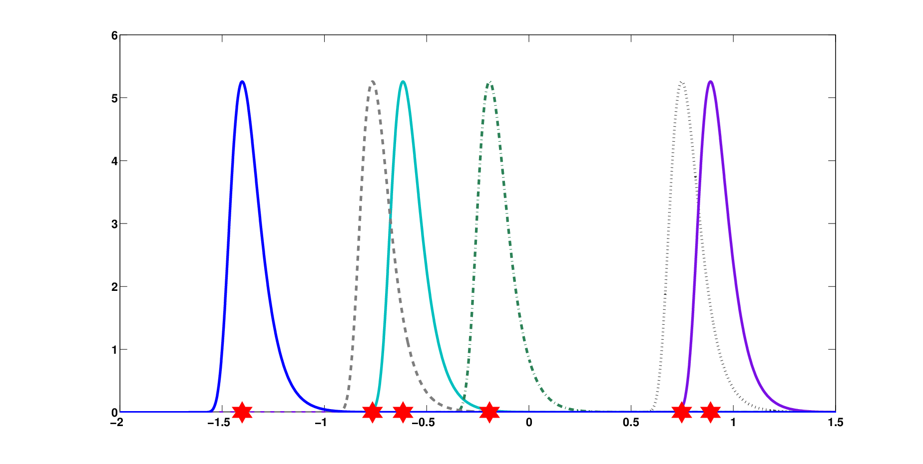
We wish to select a random permutation of the rows of , which depends only on in such a way that, after rearrangment, tend to be countermonotonic. To do so, we choose to be ranked identically to independent observations from a location family of distributions where . We might choose to be normally distributed with mean and variance or any other location family of distributions. We used following the Gumbel extreme value distribution77 7 A similar family of distributions is obtained as the logarithm of a Gamma distributed random variable and provides a random permutation from the well-known Gamma ranking family (Stern (1990)).
| (9) |
When the scale parameter of this location family approaches this ranking approaches a countermonotonic one and the algorithm approaches the Block RA. An illustration of the densities from which we simulate independently is represented in Figure 3.
Algorithm: Repeat times, with initial matrix
- 1.
Propose Determine and . For independent random variables , drawn from (9) generate a random permutation by ranking the observations . We then reorder the rows of using this permutation to obtain a proposal matrix with and leaving the columns in unchanged. The distribution of the permutation depends only on .
- 2.
Accept the proposed rearrangement of the rows of with probability proportional to otherwise do not rearrange.
- 3.
Record the states of the system having small values for and their frequencies.
We wish to identify the stationary distribution of this Markov Chain. Suppose is a matrix identical to on the columns and with columns a permutation of those of , i.e. Then the transition probability matrix is defined by:
Here, is the probability of proposing the permutation based on the row sums . The equilibrium distribution must satisfy
| (10) |
Although it may be difficult in general to solve this system of equations, provided for all this is a finite state irreducible positive recurrent (ergodic) Markov Chain. Therefore the stationary distribution is such that every state has positive probability (see Theorem, page 393, Feller (1957)). Thus it guarantees that every state is visited in finite time, and that the expected time before the chain visits the global minimum is finite. If there is a matrix such that , then the chain is absorbed and the algorithm terminates at this optimum.
This algorithm offers a compromise between rapid initial convergence and a guarantee that the global minimum variance will eventually be achieved. Depending on the choice of scale parameter, it offers a rapid convergence to a region in which the objective function is small, followed by fluctuations around the local minima of the function. Since every point in the sample space of all possible column permutations is visited with frequency proportional to we are guaranteed that the global minimum will be reached in a finite amount of time. Indeed the stationary probabilities represent the reciprocals of the mean recurrence time to this state.
Theorem 4.1.
The above algorithm generates a Markov Chain on the state space of matrices , which converges to its stationary distribution (see (10)). The probability that the global optimum is not found after simulations is for some
Proof.
The proof is a consequence of well-known results concerning the convergence of a finite state ergodic Markov Chain. For the geometric rate of convergence to the stationary distribution, see for example Cinlar (1975). ∎
We run this algorithm using as starting matrix the matrix discussed earlier, for which for all possible partitions we have that are countermonotonic so that This is a local optimum for the Block RA. The variance of the row sums is 0.04346.
| (11) |

Figure 4 illustrates the trajectory of the above algorithm for this initial matrix. Note that it successfully climbs out of local valleys and in less than 500 steps is able to find the matrix corresponding to the global minimum variance of 0. Of course the number of steps required to find this optimum is, in general, random but if we were to use enumeration, we would require evaluating the rows sums over a sample space of different matrices.
The preceding example is somewhat atypical of the performance of the algorithm because the minimum variance is and eventually this Markov Chain is absorbed in this state. When the minimum is strictly positive, the chain tends to fluctuate around its equilibrium distribution described by Theorem 4.1 above.
For example, suppose we begin with the matrix below, which was obtained by generating the first column as ordered variables and the second and third columns are random permutations of the first.
In this case, the minimizing matrix is
with variance of the row sums equal to 0.0012.
The trajectory in Figure 5 clearly shows the fluctuations around a stationary distribution in the variance of the row sums over these 5,000 iterations.

5 Conclusions
This paper proposes an improved rearrangement algorithm and a stopping rule. It can efficiently find the dependence structure that minimizes the variance of the sum of dependent variables. It is thus able to infer the dependence between variables such that the last variable is equal to the sum of the first variables. As already discussed extensively in the introduction, this idea is useful in identifying the optimal structure to achieve the Value-at-Risk bounds with a variance constraint where the aggregate risk that maximizes and minimizes the Value-at-Risk is a two-point distribution (Bernard, Rüschendorf, and Vanduffel (2016)). This idea can also be exploited in finance to infer the joint distribution among assets for which prices of spread option or basket options are available.
Acknowledgments
C. Bernard thanks the CAE research grant as well as the Alexander von Humboldt foundation and the hospitality of the chair of Mathematical Statistics in Munich where a first draft of this paper was completed in 2014. D. McLeish acknowledges support from NSERC. We would also like to thank René Carmona, Emmanuel Gobet, Giovanni Puccetti, Chris Rogers, Steven Vanduffel, Ruodu Wang and Ralf Werner for suggestions and helpful discussions on earlier drafts of this paper.
References
- Aas and Puccetti (2014) Aas, K., and G. Puccetti (2014): “Bounds on total economic capital: the DNB case study,” Extremes, 17(4), 693–715.
- Aït-Sahalia and Lo (2000) Aït-Sahalia, Y., and A. W. Lo (2000): “Nonparametric risk management and implied risk aversion,” Journal of econometrics, 94(1), 9–51.
- Alexander and Scourse (2004) Alexander, C., and A. Scourse (2004): “Bivariate normal mixture spread option valuation,” Quantitative Finance, 4(6), 637–648.
- Bernard, Jiang, and Wang (2014) Bernard, C., X. Jiang, and R. Wang (2014): “Risk aggregation with dependence uncertainty,” Insurance Mathematics and Economics, 54, 93–108.
- Bernard, Rüschendorf, and Vanduffel (2016) Bernard, C., L. Rüschendorf, and S. Vanduffel (2016): “Value-at-Risk bounds with variance constraints,” Journal of Risk and Insurance, forthcoming.
- Bernard, Rüschendorf, Vanduffel, and Yao (2016) Bernard, C., L. Rüschendorf, S. Vanduffel, and J. Yao (2016): “How robust is the value-at-risk of credit risk portfolios?,” The European Journal of Finance, forthcoming.
- Bernard and Vanduffel (2015) Bernard, C., and S. Vanduffel (2015): “A new approach to assessing model risk in high dimensions,” Journal of Banking and Finance, 58, 166–178.
- Bondarenko (2003) Bondarenko, O. (2003): “Estimation of risk-neutral densities using positive convolution approximation,” Journal of Econometrics, 116(1), 85–112.
- Breeden and Litzenberger (1978) Breeden, D. T., and R. H. Litzenberger (1978): “Prices of state-contingent claims implicit in option prices,” Journal of business, pp. 621–651.
- Carmona and Durrleman (2003) Carmona, R., and V. Durrleman (2003): “Pricing and hedging spread options,” Siam Review, 45(4), 627–685.
- Cinlar (1975) Cinlar, E. (1975): Introduction to Stochastic Processes. Springer-Verlag, New York.
- Coffman and Yannakakis (1984) Coffman, E., and M. Yannakakis (1984): “Permuting Elements within Columns of a Matrix in Order to Minimize Maximum Row Sum,” Mathematics of Operations Research, 9(3), 384–390.
- del Barrio, Cuesta-Albertos, Matrán, et al. (1999) del Barrio, E., J. A. Cuesta-Albertos, C. Matrán, et al. (1999): “Tests of goodness of fit based on the -Wasserstein distance,” The Annals of Statistics, 27(4), 1230–1239.
- Embrechts, Puccetti, and Rüschendorf (2013) Embrechts, P., G. Puccetti, and L. Rüschendorf (2013): “Model uncertainty and VaR aggregation,” Journal Banking and Finance, 37(8), 2750–2764.
- Embrechts, Puccetti, Rüschendorf, Wang, and Beleraj (2014) Embrechts, P., R. Puccetti, L. Rüschendorf, R. Wang, and A. Beleraj (2014): “An academic response to Basel 3.5,” Risks, 2(1), 25–48.
- Feller (1957) Feller, W. (1957): An Introduction to Probability Theory and Its Applications. Wiley New York.
- Hammersley and Handscomb (1964) Hammersley, J. M., and D. C. Handscomb (1964): Monte Carlo Methods, vol. 1. Springer.
- Haus (2015) Haus, U.-U. (2015): “Bounding Stochastic Dependence, Complete Mixability of Matrices, and Multidimensional Bottleneck Assignment Problems,” Operations Research Letters, 43, 74–79.
- Hsu (1984) Hsu, W.-L. (1984): “Approximation Algorithms for the Assembly Line Crew Scheduling Problem,” Mathematics of Operations Research, 9(3), 376–383.
- Krauczi (2009) Krauczi, É. (2009): “A study of the quantile correlation test for normality,” Test, 18(1), 156–165.
- Lee and Ahn (2014) Lee, W., and J. Y. Ahn (2014): “On the multidimensional extension of countermonotonicity and its applications,” Insurance: Mathematics and Economics, 56, 68–79.
- Nelsen (2006) Nelsen, R. (2006): An introduction to Copulas, vol. 2nd edition. Springer series in Statistics.
- Puccetti and Rüschendorf (2012) Puccetti, G., and L. Rüschendorf (2012): “Computation of sharp bounds on the distribution of a function of dependent risks.,” Journal of Computational and Applied Mathematics, 236(7), 1833–1840.
- Puccetti and Wang (2015a) Puccetti, G., and R. Wang (2015a): “Detecting complete and joint mixability,” Journal of Computational and Applied Mathematics, 280, 174–187.
- Puccetti and Wang (2015b) (2015b): “Extremal dependence concepts,” Statistical Science, 30(4), 485–517.
- Rosenberg (2000) Rosenberg, J. V. (2000): “Nonparametric pricing of multivariate contingent claims,” NYU Working Paper No. FIN-00-001.
- Stern (1990) Stern, H. (1990): “Models for distributions on permutations,” Journal of the American Statistical Association, 85(410), 558–564.
- Wang and Wang (2011) Wang, B., and R. Wang (2011): “The complete mixability and convex minimization problems with monotone marginal densities,” Journal of Multivariate Analysis, 102(10), 1344–1360.
- Wang and Wang (2016) Wang, B., and R. Wang (2016): “Joint mixability,” Mathematics of Operations Research, forthcoming.