Massively Multitask Networks for Drug Discovery

Bharath Ramsundar^{*, $\dagger$ , $\circ$} Steven Kearnes^{*, $\dagger$} Patrick Riley^$\circ$ Dale Webster^$\circ$ David Konerding^$\circ$ Vijay Pande^$\dagger$ Address: (^*Equal contribution, ^$\dagger$Stanford University, ^$\circ$Google Inc.)

Abstract

Massively multitask neural architectures provide a learning framework for drug discovery that synthesizes information from many distinct biological sources. To train these architectures at scale, we gather large amounts of data from public sources to create a dataset of nearly 40 million measurements across more than 200 biological targets. We investigate several aspects of the multitask framework by performing a series of empirical studies and obtain some interesting results: $(1)$ massively multitask networks obtain predictive accuracies significantly better than single-task methods, $(2)$ the predictive power of multitask networks improves as additional tasks and data are added, $(3)$ the total amount of data and the total number of tasks both contribute significantly to multitask improvement, and $(4)$ multitask networks afford limited transferability to tasks not in the training set. Our results underscore the need for greater data sharing and further algorithmic innovation to accelerate the drug discovery process.

Keywords:

deep learning, bioinformatics

1 Introduction

Discovering new treatments for human diseases is an immensely complicated challenge. Prospective drugs must attack the source of an illness, but must do so while satisfying restrictive metabolic and toxicity constraints. Traditionally, drug discovery is an extended process that takes years to move from start to finish, with high rates of failure along the way.

After a suitable target has been identified, the first step in the drug discovery process is “hit finding.” Given some druggable target, pharmaceutical companies will screen millions of drug-like compounds in an effort to find a few attractive molecules for further optimization. These screens are often automated via robots, but are expensive to perform. Virtual screening attempts to replace or augment the high-throughput screening process by the use of computational methods (Shoichet, 2004). Machine learning methods have frequently been applied to virtual screening by training supervised classifiers to predict interactions between targets and small molecules.

There are a variety of challenges that must be overcome to achieve effective virtual screening. Low hit rates in experimental screens (often only $1$ – $2$ % of screened compounds are active against a given target) result in imbalanced datasets that require special handling for effective learning. For instance, care must be taken to guard against unrealistic divisions between active and inactive compounds (“artificial enrichment”) and against information leakage due to strong similarity between active compounds (“analog bias”) (Rohrer & Baumann, 2009). Furthermore, the paucity of experimental data means that overfitting is a perennial thorn.

The overall complexity of the virtual screening problem has limited the impact of machine learning in drug discovery. To achieve greater predictive power, learning algorithms must combine disparate sources of experimental data across multiple targets. Deep learning provides a flexible paradigm for synthesizing large amounts of data into predictive models. In particular, multitask networks facilitate information sharing across different experiments and compensate for the limited data associated with any particular experiment.

In this work, we investigate several aspects of the multitask learning paradigm as applied to virtual screening. We gather a large collection of datasets containing nearly 40 million experimental measurements for over 200 targets. We demonstrate that multitask networks trained on this collection achieve significant improvements over baseline machine learning methods. We show that adding more tasks and more data yields better performance. This effect diminishes as more data and tasks are added, but does not appear to plateau within our collection. Interestingly, we find that the total amount of data and the total number of tasks both have significant roles in this improvement. Furthermore, the features extracted by the multitask networks demonstrate some transferability to tasks not contained in the training set. Finally, we find that the presence of shared active compounds is moderately correlated with multitask improvement, but the biological class of the target is not.

2 Related Works

Machine learning has a rich history in drug discovery. Early work combined creative featurizations of molecules with off-the-shelf learning algorithms to predict drug activity (Varnek & Baskin, 2012). The state of the art has moved to more refined models, such as the influence relevance voting method that combines low-complexity neural networks and k-nearest neighbors (Swamidass et al., 2009), and Bayesian belief networks that repurpose textual information retrieval methods for virtual screening (Abdo et al., 2010). Other related work uses deep recursive neural networks to predict aqueous solubility by extracting features from the connectivity graphs of small molecules (Lusci et al., 2013).

Deep learning has made inroads into drug discovery in recent years, most notably in 2012 with the Merck Kaggle competition (Dahl, November 1, 2012). Teams were given pre-computed molecular descriptors for compounds with experimentally measured activity against 15 targets and were asked to predict the activity of molecules in a held-out test set. The winning team used ensemble models including multitask deep neural networks, Gaussian process regression, and dropout to improve the baseline test set $R^{2}$ by nearly 17%. The winners of this contest later released a technical report that discusses the use of multitask networks for virtual screening (Dahl et al., 2014). Additional work at Merck analyzed the choice of hyperparameters when training single- and multitask networks and showed improvement over random forest models (Ma et al., 2015). The Merck Kaggle result has been received with skepticism by some in the cheminformatics and drug discovery communities (Lowe, December 11, 2012, and associated comments). Two major concerns raised were that the sample size was too small (a good result across 15 systems may well have occurred by chance) and that any gains in predictive accuracy were too small to justify the increase in complexity.

While we were preparing this work, a workshop paper was released that also used massively multitask networks for virtual screening (Unterthiner et al., ). That work curated a dataset of 1,280 biological targets with 2 million associated data points and trained a multitask network. Their network has more tasks than ours (1,280 vs. 259) but far fewer data points (2 million vs. nearly 40 million). The emphasis of our work is considerably different; while their report highlights the performance gains due to multitask networks, ours is focused on disentangling the underlying causes of these improvements. Another closely related work proposed the use of collaborative filtering for virtual screening and employed both multitask networks and kernel-based methods (Erhan et al., 2006). Their multitask networks, however, did not consistently outperform single-task models.

Within the greater context of deep learning, we draw upon various strands of recent thought. Prior work has used multitask deep networks in the contexts of language understanding (Collobert & Weston, 2008) and multi-language speech recognition (Deng et al., 2013). Our best-performing networks draw upon design patterns introduced by GoogLeNet (Szegedy et al., 2014), the winner of ILSVRC 2014.

3 Methods

3.1 Dataset Construction and Design

Models were trained on $259$ datasets gathered from publicly available data. These datasets were divided into four groups: PCBA, MUV, DUD-E, and Tox21. The PCBA group contained $128$ experiments in the PubChem BioAssay database (Wang et al., 2012). The MUV group contained $17$ challenging datasets specifically designed to avoid common pitfalls in virtual screening (Rohrer & Baumann, 2009). The DUD-E group contained $102$ datasets that were designed for the evaluation of methods to predict interactions between proteins and small molecules (Mysinger et al., 2012). The Tox21 datasets were used in the recent Tox21 Data Challenge (https://tripod.nih.gov/tox21/challenge/) and contained experimental data for $12$ targets relevant to drug toxicity prediction. We used only the training data from this challenge because the test set had not been released when we constructed our collection. In total, our $259$ datasets contained $37.8$ M experimental data points for $1.6$ M compounds. Details for the dataset groups are given in Table 1. See the Appendix for details on individual datasets and their biological target categorization.

Table 1: Details for dataset groups. Values for the number of data points per dataset and the percentage of active compounds are reported as means, with standard deviations in parenthesis.

Group	Datasets	Data Points / ea.	% Active
PCBA	128	$282\text{K}$ $(122\text{K})$	$1.8$ $(3.8)$
DUD-E	$102$	$14\text{K}$ $(11\text{K})$	$1.6$ $(0.2)$
MUV	$17$	$15\text{K}$ $(1)$	$0.2$ $(0)$
Tox21	$12$	$6\text{K}$ $(500)$	$7.8$ $(4.7)$

It should be noted that we did not perform any preprocessing of our datasets, such as removing potential experimental artifacts. Such artifacts may be due by compounds whose physical properties cause interference with experimental measurements or allow for promiscuous interactions with many targets. A notable exception is the MUV group, which has been processed with consideration of these pathologies (Rohrer & Baumann, 2009).

3.2 Small Molecule Featurization

We used extended connectivity fingerprints (ECFP4) (Rogers & Hahn, 2010) generated by RDKit (Landrum, ) to featurize each molecule. The molecule is decomposed into a set of fragments—each centered at a non-hydrogen atom—where each fragment extends radially along bonds to neighboring atoms. Each fragment is assigned a unique identifier, and the collection of identifiers for a molecule is hashed into a fixed-length bit vector to construct the molecular “fingerprint”. ECFP4 and other fingerprints are commonly used in cheminformatics applications, especially to measure similarity between compounds (Willett et al., 1998). A number of molecules (especially in the Tox21 group) failed the featurization process and were not used in training our networks. See the Appendix for details.

3.3 Validation Scheme and Metrics

The traditional approach for model evaluation is to have fixed training, validation, and test sets. However, the imbalance present in our datasets means that performance varies widely depending on the particular training/test split. To compensate for this variability, we used stratified $K$ -fold cross-validation; that is, each fold maintains the active/inactive proportion present in the unsplit data. For the remainder of the paper, we use $K=5$ .

Note that we did not choose an explicit validation set. Several datasets in our collection have very few actives ( $\sim 30$ each for the MUV group), and we feared that selecting a specific validation set would skew our results. As a consequence, we suspect that our choice of hyperparameters may be affected by information leakage across folds. However, our networks do not appear to be highly sensitive to hyperparameter choice (see Section 4.1), so we do not consider leakage to be a serious issue.

Following recommendations from the cheminformatics community (Jain & Nicholls, 2008), we used metrics derived from the receiver operating characteristic (ROC) curve to evaluate model performance. Recall that the ROC curve for a binary classifier is the plot of true positive rate (TPR) vs. false positive rate (FPR) as the discrimination threshold is varied. For individual datasets, we are interested in the area under the ROC curve (AUC), which is a global measure of classification performance (note that AUC must lie in the range $[0,1]$ ). More generally, for a collection of $N$ datasets, we consider the mean and median $K$ -fold-average AUC:

\Mean/\Median\left\{\frac{1}{K}\sum_{k=1}^{K}\text{AUC}_{k}(D_{n})\middle|\ n=1,\dotsc,N\right\},

where $\text{AUC}_{k}(D_{n})$ is defined as the AUC of a classifier trained on folds $\{1,\dotsc,K\}\setminus k$ of dataset $D_{n}$ and tested on fold $k$ . For completeness, we include in the Appendix an alternative metric called “enrichment” that is widely used in the cheminformatics literature (Jain & Nicholls, 2008). We note that many other performance metrics exist in the literature; the lack of standard metrics makes it difficult to do direct comparisons with previous work.

3.4 Multitask Networks

A neural network is a nonlinear classifier that performs repeated linear and nonlinear transformations on its input. Let $\mathbf{x}_{i}$ represent the input to the $i$ -th layer of the network (where $\mathbf{x}_{0}$ is simply the feature vector). The transformation performed is

\mathbf{x}_{i+1}=\sigma(\mathbf{W}_{i}\mathbf{x}_{i}+\mathbf{b}_{i})

where $\mathbf{W}_{i}$ and $\mathbf{b}_{i}$ are respectively the weight matrix and bias for the $i$ -th layer, and $\sigma$ is a nonlinearity (in our work, the rectified linear unit (Nair & Hinton, 2010)). After $L$ such transformations, the final layer of the network $\mathbf{x}_{L}$ is then fed to a simple linear classifier, such as the softmax, which predicts the probability that the input $\mathbf{x}_{0}$ has label $j$ :

P(y=j|\mathbf{x}_{0})=\frac{e^{(\mathbf{w}^{j})^{T}\mathbf{x}_{L}}}{\sum_{m=1}^{M}e^{(\mathbf{w}^{m})^{T}\mathbf{x}_{L}}},

where $M$ is the number of possible labels (here $M=2$ ) and $\mathbf{w}^{1},\cdots,\mathbf{w}^{M}$ are weight vectors. $\mathbf{W}_{i}$ , $\mathbf{b}_{i}$ , and $\mathbf{w}^{m}$ are learned during training by the backpropagation algorithm (Rumelhart et al., 1988). A multitask network attaches $N$ softmax classifiers, one for each task, to the final layer $\mathbf{x}_{L}$ . (A “task” corresponds to the classifier associated with a particular dataset in our collection, although we often use “task” and “dataset” interchangeably. See Figure 1.)

Figure 1: Multitask neural network.

4 Experimental Section

In this section, we seek to answer a number of questions about the performance, capabilities, and limitations of massively multitask neural networks:

1.

Do massively multitask networks provide a performance boost over simple machine learning methods? If so, what is the optimal architecture for massively multitask networks?
2.

How does the performance of a multitask network depend on the number of tasks? How does the performance depend on the total amount of data?
3.

Do massively multitask networks extract generalizable information about chemical space?
4.

When do datasets benefit from multitask training?

The following subsections detail a series of experiments that seek to answer these questions.

4.1 Experimental Exploration of Massively Multitask Networks

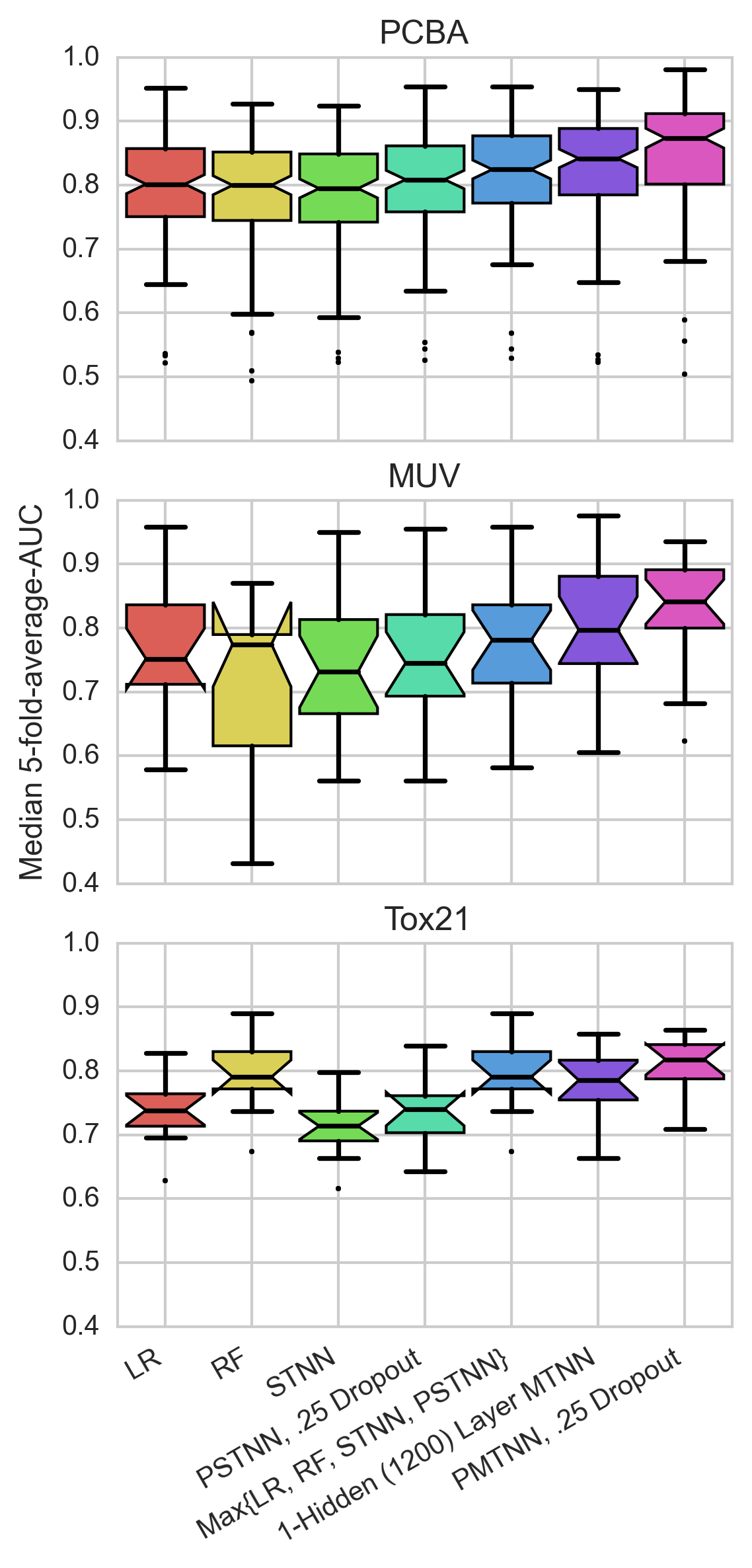
We investigate the performance of multitask networks with various hyperparameters and compare to several standard machine learning approaches. Table 2 shows some of the highlights of our experiments. Our best multitask architecture (pyramidal multitask networks) significantly outperformed simpler models, including a hypothetical model whose performance on each dataset matches that of the best single-task model (Max{LR, RF, STNN, PSTNN}).

Every model we trained performed extremely well on the DUD-E datasets (all models in Table 2 had median $5$ -fold-average AUCs $\geq 0.99$ ), making comparisons between models on DUD-E uninformative. For that reason, we exclude DUD-E from our subsequent statistical analysis. However, we did not remove DUD-E from the training altogether because doing so adversely affected performance on the other datasets (data not shown); we theorize that DUD-E helped to regularize the classifier and avoid overfitting.

Table 2: Median

5

-fold-average AUCs for various models. For each model, the sign test in the last column estimates the fraction of datasets (excluding the DUD-E group, for reasons discussed in the text) for which that model is superior to the PMTNN (bottom row). We use the Wilson score interval to derive a

95\%

confidence interval for this fraction. Non-neural network methods were trained using scikit-learn (Pedregosa et al., 2011) implementations and basic hyperparameter optimization. We also include results for a hypothetical “best” single-task model (Max{LR, RF, STNN, PSTNN}) to provide a stronger baseline. Details for our cross-validation and training procedures are given in the Appendix.

Model	PCBA $(n=128)$	MUV $(n=17)$	Tox21 $(n=12)$	Sign Test CI
Logistic Regression (LR)	$.801$	$.752$	$.738$	$[.04,.13]$
Random Forest (RF)	$.800$	$.774$	$.790$	$[.06,.16]$
Single-Task Neural Net (STNN)	$.795$	$.732$	$.714$	$[.04,.12]$
Pyramidal $(2000,100)$ STNN (PSTNN)	.809	.745	.740	$[.06,.16]$
Max{LR, RF, STNN, PSTNN}	$.824$	$.781$	$.790$	$[.12,.24]$
$1$ -Hidden $(1200)$ Layer Multitask Neural Net (MTNN)	$.842$	$.797$	$.785$	$[.08,.18]$
Pyramidal $(2000,100)$ Multitask Neural Net (PMTNN)	$\mathbf{.873}$	$\mathbf{.841}$	$\mathbf{.818}$

During our first explorations, we had consistent problems with the networks overfitting the data. As discussed in Section 3.1, our datasets had a very small fraction of positive examples. For the single hidden layer multitask network in Table 2, each dataset had $1200$ associated parameters. With a total number of positives in the tens or hundreds, overfitting this number of parameters is a major issue in the absence of strong regularization.

Reducing the number of parameters specific to each dataset is the motivation for the pyramidal architecture. In our pyramidal networks, the first hidden layer is very wide ( $2000$ nodes) with a second narrow hidden layer ( $100$ nodes). This dimensionality reduction is similar in motivation and implementation to the $1$ x $1$ convolutions in the GoogLeNet architecture (Szegedy et al., 2014). The wide lower layer allows for complex, expressive features to be learned while the narrow layer limits the parameters specific to each task. Adding dropout of $0.25$ to our pyramidal networks improved performance. We also trained single-task versions of our best pyramidal network to understand whether this design pattern works well with less data. Table 2 indicates that these models outperform vanilla single-task networks but do not substitute for multitask training. Results for a variety of alternate models are presented in the Appendix.

We investigated the sensitivity of our results to the sizes of the pyramidal layers by running networks with all combinations of hidden layer sizes: $(1000,2000,3000)$ and $(50,100,150)$ . Across the architectures, means and medians shifted by $\leq.01$ AUC with only MUV showing larger changes with a range of $.038$ . We note that performance is sensitive to the choice of learning rate and the number of training steps. See the Appendix for details and data.

4.2 Relationship between performance and number of tasks

The previous section demonstrated that massively multitask networks improve performance over single-task models. In this section, we seek to understand how multitask performance is affected by increasing the number of tasks. A priori, there are three reasonable “growth curves” (visually represented in Figure 2):

Over the hill:: performance initially improves, hits a maximum, then falls.
Plateau:: performance initially improves, then plateaus.
Still climbing:: performance improves throughout, but with a diminishing rate of return.

Refer to caption — Figure 2: Potential multitask growth curves

We constructed and trained a series of multitask networks on datasets containing $10,20,40,80,160,$ and $249$ tasks. These datasets all contain a fixed set of ten “held-in” tasks, which consists of a randomly sampled collection of five PCBA, three MUV, and two Tox21 datasets. These datasets correspond to unique targets that do not have any obvious analogs in the remaining collection. (We also excluded a similarly chosen set of ten “held-out” tasks for use in Section 4.4). Each training collection is a superset of the preceding collection, with tasks added randomly. For each network in the series, we computed the mean $5$ -fold-average-AUC for the tasks in the held-in collection. We repeated this experiment ten times with different choices of random seed.

Figure 3: Held-in growth curves. The

y

-axis shows the change in AUC compared to a single-task neural network with the same architecture (PSTNN). Each colored curve is the multitask improvement for a given held-in dataset. Black dots represent means across the

10

held-in datasets for each experimental run, where additional tasks were randomly selected. The shaded curve is the mean across the

100

combinations of datasets and experimental runs.

Figure 3 plots the results of our experiments. The shaded region emphasizes the average growth curve, while black dots indicate average results for different experimental runs. The figure also displays lines associated with each held-in dataset. Note that several datasets show initial dips in performance. However, all datasets show subsequent improvement, and all but one achieves performance superior to the single-task baseline. Within the limits of our current dataset collection, the distribution in Figure 3 agrees with either plateau or still climbing. The mean performance on the held-in set is still increasing at $249$ tasks, so we hypothesize that performance is still climbing. It is possible that our collection is too small and that an alternate pattern may eventually emerge.

4.3 More tasks or more data?

In the previous section we studied the effects of adding more tasks, but here we investigate the relative importance of the total amount of data vs. the total number of tasks. Namely, is it better to have many tasks with a small amount of associated data, or a small number of tasks with a large amount of associated data?

We constructed a series of multitask networks with $10,15,20,30,50$ and $82$ tasks. As in the previous section, the tasks are randomly associated with the networks in a cumulative manner (i.e., the $82$ -task network contained all tasks present in the $50$ -task network, and so on). All networks contained the ten held-in tasks described in the previous section. The $82$ tasks chosen were associated with the largest datasets in our collection, each containing $300$ K- $500$ K data points. Note that all of these tasks belonged to the PCBA group.

We then trained this series of networks multiple times with $1.6$ M, $3.3$ M, $6.5$ M, $13$ M, and $23$ M data points sampled from the non-held-in tasks. We perform the sampling such that for a given task, all data points present in the first stage ( $1.6$ M) appeared in the second ( $3.3$ M), all data points present in the second stage appeared in the third ( $6.5$ M), and so on. We decided to use larger datasets so we could sample meaningfully across this entire range. Some combinations of tasks and data points were not realized; for instance, we did not have enough data to train a $20$ -task network with $23$ M additional data points. We repeated this experiment ten times using different random seeds.

Figure 4 shows the results of our experiments. The $x$ -axis tracks the number of additional tasks, while the $y$ -axis displays the improvement in performance for the held-in set relative to a multitask network trained only on the held-in data. When the total amount of data is fixed, having more tasks consistently yields improvement. Similarly, when the number of tasks is fixed, adding additional data consistently improves performance. Our results suggest that the total amount of data and the total number of tasks both contribute significantly to the multitask effect.

Figure 4: Multitask benefit from increasing tasks and data independently. As in Figure 2, we added randomly selected tasks (

x

-axis) to a fixed held-in set. A stratified random sampling scheme was applied to the additional tasks in order to achieve fixed total numbers of additional input examples (color, line type). White points indicate the mean over

10

experimental runs of

\Delta

mean-AUC over the initial network trained on the

10

held-in datasets. Color-filled areas and error bars describe the smoothed

95\%

confidence intervals.

4.4 Do massively multitask networks extract generalizable features?

The features extracted by the top layer of the network represent information useful to many tasks. Consequently, we sought to determine the transferability of these features to tasks not in the training set. We held out ten data sets from the growth curves calculated in Section 4.2 and used the learned weights from points along the growth curves to initialize single-task networks for the held-out datasets, which we then fine-tuned.

The results of training these networks (with $5$ -fold stratified cross-validation) are shown in Figure 5. First, note that many of the datasets performed worse than the baseline when initialized from the 10-held-in-task networks. Further, some datasets never exhibited any positive effect due to multitask initialization. Transfer learning can be negative.

Second, note that the transfer learning effect became stronger as multitask networks were trained on more data. Large multitask networks exhibited better transferability, but the average effect even with $249$ datasets was only $\sim.01$ AUC. We hypothesize that the extent of this generalizability is determined by the presence or absence of relevant data in the multitask training set.

Figure 5: Held-out growth curves. The

y

-axis shows the change in AUC compared to a single-task neural network with the same architecture (PSTNN). Each colored curve is the result of initializing a single-task neural network from the weights of the networks from Section 4.2 and computing the mean across the

10

experimental runs. These datasets were not included in the training of the original networks. The shaded curve is the mean across the

100

combinations of datasets and experimental runs, and black dots represent means across the

10

held-out datasets for each experimental run, where additional tasks were randomly selected.

4.5 When do datasets benefit from multitask training?

The results in Sections 4.2 and 4.4 indicate that some datasets benefit more from multitask training than others. In an effort to explain these differences, we consider three specific questions:

1.

Do shared active compounds explain multitask improvement?
2.

Do some biological target classes realize greater multitask improvement than others?
3.

Do tasks associated with duplicated targets have artificially high multitask performance?

4.5.1 Shared Active Compounds

The biological context of our datasets implies that active compounds contain more information than inactive compounds; while an inactive compound may be inactive for many reasons, active compounds often rely on similar physical mechanisms. Hence, shared active compounds should be a good measure of dataset similarity.

Figure 6 plots multitask improvement against a measure of dataset similarity we call “active occurrence rate” (AOR). For each active compound $\alpha$ in dataset $D_{i}$ , $\text{AOR}_{i,\alpha}$ is defined as the number of additional datasets in which this compound is also active:

\text{AOR}_{i,\alpha}=\sum_{d\neq i}\mathbbm{1}{\left(\alpha\in\text{Actives}\left(D_{d}\right)\right)}.

Each point in Figure 6 corresponds to a single dataset $D_{i}$ . The $x$ -coordinate is

\text{AOR}_{i}=\Mean_{\alpha\in\text{Actives}\left(D_{i}\right)}\left(\text{AOR}_{i,\alpha}\right),

and the $y$ -coordinate ( $\Delta$ log-odds-mean-AUC) is

\small\text{logit}\left(\frac{1}{K}\sum_{k=1}^{K}\text{AUC}_{k}^{(M)}\left(D_{i}\right)\right)-\text{logit}\left(\frac{1}{K}\sum_{k=1}^{K}\text{AUC}_{k}^{(S)}\left(D_{i}\right)\right),

where $\text{AUC}_{k}^{(M)}\left(D_{i}\right)$ and $\text{AUC}_{k}^{(S)}\left(D_{i}\right)$ are respectively the AUC values for the $k$ -th fold of dataset $i$ in the multitask and single-task models, and $\text{logit}\left(p\right)=\log\left(p/(1-p)\right)$ . The use of log-odds reduces the effect of outliers and emphasizes changes in AUC when the baseline is high. Note that for reasons discussed in Section 4.1, DUD-E was excluded from this analysis.

There is a moderate correlation between AOR and $\Delta$ log-odds-mean-AUC ( $r^{2}=.33$ ); we note that this correlation is not present when we use $\Delta$ mean-AUC as the $y$ -coordinate ( $r^{2}=.09$ ). We hypothesize that some portion of the multitask effect is determined by shared active compounds. That is, a dataset is most likely to benefit from multitask training when it shares many active compounds with other datasets in the collection.

4.5.2 Target Classes

Figure 7 shows the relationship between multitask improvement and target classes. As before, we report multitask improvement in terms of log-odds and exclude the DUD-E datasets. Qualitatively, no target class benefited more than any other from multitask training. Nearly every target class realized gains, suggesting that the multitask framework is applicable to experimental data from multiple target classes.

4.5.3 Duplicate Targets

As mentioned in Section 3.1, there are many cases of tasks with identical targets. We compared the multitask improvement of duplicate vs. unique tasks. The distributions have substantial overlap (see the Appendix), but the average log-odds improvement was slightly higher for duplicated tasks ( $.531$ vs. $.372$ ; a one-sided $t$ -test between the duplicate and unique distributions gave $p=.016$ ). Since duplicated targets are likely to share many active compounds, this improvement is consistent with the correlation seen in Section 4.5.1. However, sign tests for single-task vs. multitask models for duplicate and unique targets gave significant and highly overlapping confidence intervals ( $[0.04,0.24]$ and $[0.06,0.17]$ , respectively; recall that the meaning of these intervals is given in the caption for Table 2). Together, these results suggest that there is not significant information leakage within multitask networks. Consequently, the results of our analysis are unlikely to be significantly affected by the presence of duplicate targets in our dataset collection.

5 Discussion and Conclusion

In this work, we investigated the use of massively multitask networks for virtual screening. We gathered a large collection of publicly available experimental data that we used to train massively multitask neural networks. These networks achieved significant improvement over simple machine learning algorithms.

We explored several aspects of the multitask framework. First, we demonstrated that multitask performance improved with the addition of more tasks; our performance was still climbing at 259 tasks. Next, we considered the relative importance of introducing more data vs. more tasks. We found that additional data and additional tasks both contributed significantly to the multitask effect. We next discovered that multitask learning afforded limited transferability to tasks not contained in the training set. This effect was not universal, and required large amounts of data even when it did apply.

We observed that the multitask effect was stronger for some datasets than others. Consequently, we investigated possible explanations for this discrepancy and found that the presence of shared active compounds was moderately correlated with multitask improvement, but the biological class of the target was not. It is also possible that multitask improvement results from accurately modeling experimental artifacts rather than specific interactions between targets and small molecules. We do not believe this to be the case, as we demonstrated strong improvement on the thoroughly-cleaned MUV datasets.

The efficacy of multitask learning is directly related to the availability of relevant data. Hence, obtaining greater amounts of data is of critical importance for improving the state of the art. Major pharmaceutical companies possess vast private stores of experimental measurements; our work provides a strong argument that increased data sharing could result in benefits for all.

More data will maximize the benefits achievable using current architectures, but in order for algorithmic progress to occur, it must be possible to judge the performance of proposed models against previous work. It is disappointing to note that all published applications of deep learning to virtual screening (that we are aware of) use distinct datasets that are not directly comparable. It remains to future research to establish standard datasets and performance metrics for this field.

Another direction for future work is the further study of small molecule featurization. In this work, we use only one possible featurization (ECFP4), but there exist many others. Additional performance may also be realized by considering targets as well as small molecules in the featurization. Yet another line of research could improve performance by using unsupervised learning to explore much larger segments of chemical space.

Although deep learning offers interesting possibilities for virtual screening, the full drug discovery process remains immensely complicated. Can deep learning—coupled with large amounts of experimental data—trigger a revolution in this field? Considering the transformational effect that these methods have had on other fields, we are optimistic about the future.

Acknowledgments

B.R. was supported by the Fannie and John Hertz Foundation. S.K. was supported by a Smith Stanford Graduate Fellowship. We also acknowledge support from NIH and NSF, in particular NIH U54 GM072970 and NSF 0960306. The latter award was funded under the American Recovery and Reinvestment Act of 2009 (Public Law 111-5).

References

Abdo et al. (2010) Abdo, Ammar, Chen, Beining, Mueller, Christoph, Salim, Naomie, and Willett, Peter. Ligand-based virtual screening using bayesian networks. Journal of chemical information and modeling, 50(6):1012–1020, 2010.
Collobert & Weston (2008) Collobert, Ronan and Weston, Jason. A unified architecture for natural language processing: Deep neural networks with multitask learning. In Proceedings of the 25th international conference on Machine learning, pp. 160–167. ACM, 2008.
Dahl (November 1, 2012) Dahl, George. Deep Learning How I Did It: Merck 1st place interview. No Free Hunch, November 1, 2012.
Dahl et al. (2014) Dahl, George E, Jaitly, Navdeep, and Salakhutdinov, Ruslan. Multi-task neural networks for QSAR predictions. arXiv preprint arXiv:1406.1231, 2014.
Deng et al. (2013) Deng, Li, Hinton, Geoffrey, and Kingsbury, Brian. New types of deep neural network learning for speech recognition and related applications: An overview. In Acoustics, Speech and Signal Processing (ICASSP), 2013 IEEE International Conference on, pp. 8599–8603. IEEE, 2013.
Erhan et al. (2006) Erhan, Dumitru, L’Heureux, Pierre-Jean, Yue, Shi Yi, and Bengio, Yoshua. Collaborative filtering on a family of biological targets. Journal of chemical information and modeling, 46(2):626–635, 2006.
Jain & Nicholls (2008) Jain, Ajay N and Nicholls, Anthony. Recommendations for evaluation of computational methods. Journal of computer-aided molecular design, 22(3-4):133–139, 2008.
(8) Landrum, Greg. RDKit: Open-source cheminformatics. URL http://www.rdkit.org.
Lowe (December 11, 2012) Lowe, Derek. Did Kaggle Predict Drug Candidate Activities? Or Not? In the Pipeline, December 11, 2012.
Lusci et al. (2013) Lusci, Alessandro, Pollastri, Gianluca, and Baldi, Pierre. Deep architectures and deep learning in chemoinformatics: the prediction of aqueous solubility for drug-like molecules. Journal of chemical information and modeling, 53(7):1563–1575, 2013.
Ma et al. (2015) Ma, Junshui, Sheridan, Robert P, Liaw, Andy, Dahl, George, and Svetnik, Vladimir. Deep neural nets as a method for quantitative structure-activity relationships. Journal of Chemical Information and Modeling, 2015.
Mysinger et al. (2012) Mysinger, Michael M, Carchia, Michael, Irwin, John J, and Shoichet, Brian K. Directory of useful decoys, enhanced (DUD-E): better ligands and decoys for better benchmarking. Journal of medicinal chemistry, 55(14):6582–6594, 2012.
Nair & Hinton (2010) Nair, Vinod and Hinton, Geoffrey E. Rectified linear units improve restricted boltzmann machines. In Proceedings of the 27th International Conference on Machine Learning (ICML-10), pp. 807–814, 2010.
Pedregosa et al. (2011) Pedregosa, Fabian, Varoquaux, Gaël, Gramfort, Alexandre, Michel, Vincent, Thirion, Bertrand, Grisel, Olivier, Blondel, Mathieu, Prettenhofer, Peter, Weiss, Ron, Dubourg, Vincent, et al. Scikit-learn: Machine learning in python. The Journal of Machine Learning Research, 12:2825–2830, 2011.
Rogers & Hahn (2010) Rogers, David and Hahn, Mathew. Extended-connectivity fingerprints. Journal of chemical information and modeling, 50(5):742–754, 2010.
Rohrer & Baumann (2009) Rohrer, Sebastian G and Baumann, Knut. Maximum unbiased validation (MUV) data sets for virtual screening based on pubchem bioactivity data. Journal of chemical information and modeling, 49(2):169–184, 2009.
Rumelhart et al. (1988) Rumelhart, David E, Hinton, Geoffrey E, and Williams, Ronald J. Learning representations by back-propagating errors. Cognitive modeling, 1988.
Shoichet (2004) Shoichet, Brian K. Virtual screening of chemical libraries. Nature, 432(7019):862–865, 2004.
Swamidass et al. (2009) Swamidass, S Joshua, Azencott, Chloé-Agathe, Lin, Ting-Wan, Gramajo, Hugo, Tsai, Shiou-Chuan, and Baldi, Pierre. Influence relevance voting: an accurate and interpretable virtual high throughput screening method. Journal of chemical information and modeling, 49(4):756–766, 2009.
Szegedy et al. (2014) Szegedy, Christian, Liu, Wei, Jia, Yangqing, Sermanet, Pierre, Reed, Scott, Anguelov, Dragomir, Erhan, Dumitru, Vanhoucke, Vincent, and Rabinovich, Andrew. Going deeper with convolutions. arXiv preprint arXiv:1409.4842, 2014.
(21) Unterthiner, Thomas, Mayr, Andreas, ünter Klambauer, G, Steijaert, Marvin, Wenger, Jörg, Ceulemans, Hugo, and Hochreiter, Sepp. Deep learning as an opportunity in virtual screening.
Varnek & Baskin (2012) Varnek, Alexandre and Baskin, Igor. Machine learning methods for property prediction in chemoinformatics: quo vadis? Journal of chemical information and modeling, 52(6):1413–1437, 2012.
Wang et al. (2012) Wang, Yanli, Xiao, Jewen, Suzek, Tugba O, Zhang, Jian, Wang, Jiyao, Zhou, Zhigang, Han, Lianyi, Karapetyan, Karen, Dracheva, Svetlana, Shoemaker, Benjamin A, et al. PubChem’s BioAssay database. Nucleic acids research, 40(D1):D400–D412, 2012.
Willett et al. (1998) Willett, Peter, Barnard, John M, and Downs, Geoffrey M. Chemical similarity searching. Journal of chemical information and computer sciences, 38(6):983–996, 1998.

A Dataset Construction and Design

The PCBA datasets are dose-response assays performed by the NCATS Chemical Genomics Center (NCGC) and downloaded from PubChem BioAssay using the following search limits: TotalSidCount from 10000, ActiveSidCount from 30, Chemical, Confirmatory, Dose-Response, Target: Single, NCGC. These limits correspond to the search query: (10000[TotalSidCount] : 1000000000[TotalSidCount]) AND (30[ActiveSidCount] : 1000000000[ActiveSidCount]) AND “small_molecule”[filt] AND “doseresponse”[filt] AND 1[TargetCount] AND “NCGC”[SourceName]. We note that the DUD-E datasets are especially susceptible to “artificial enrichment” (unrealistic divisions between active and inactive compounds) as an artifact of the dataset construction procedure. Each data point in our collection was associated with a binary label classifying it as either active or inactive.

A description of each of our 259 datasets is given in Table A1. These datasets cover a wide range of target classes and assay types, including both cell-based and in vitro experiments. Datasets with duplicated targets are marked with an asterisk (note that only the non-DUD-E duplicate target datasets were used in the analysis described in the text). For the PCBA datasets, compounds not labeled “Active” were considered inactive (including compounds marked “Inconclusive”). Due to missing data in PubChem BioAssay and/or featurization errors, some data points and compounds were not used for evaluation of our models; failure rates for each dataset group are shown in Table A.1. The Tox21 group suffered especially high failure rates, likely due to the relatively large number of metallic or otherwise abnormal compounds that are not supported by the RDKit package. The counts given in Table A1 do not include these missing data. A graphical breakdown of the datasets by target class is shown in Figure A.1. The datasets used for the held-in and held-out analyses are repeated in Table A.2 and Table A.3, respectively.

As an extension of our treatment of task similarity in the text, we generated the heatmap in Figure A.2 to show the pairwise intersection between all datasets in our collection. A few characteristics of our datasets are immediately apparent:

•

The datasets in the DUD-E group have very little intersection with any other datasets.
•

The PCBA and Tox21 datasets have substantial self-overlap. In contrast, the MUV datasets have relatively little self-overlap.
•

The MUV datasets have substantial overlap with the datasets in the PCBA group.
•

The Tox21 datasets have very small intersections with datasets in other groups.

Figure A.3 shows the $\Delta$ log-odds-mean-AUC for datasets with duplicate and unique targets.

\csvreader

[ longtable=lSSp1inp1.9in, table head=Dataset Actives Inactives Target Class Target
\endhead\endfoot, ] datasets.csv1=\Dataset, 2=\Actives, 3=\Inactives, 4=\Class, 5=\Target\Dataset \Actives \Inactives \Class \Target

Table A.1: Featurization failures.

Group	Original	Featurized	Failure Rate (%)
PCBA	$439\,879$	$437\,928$	$0.44$
DUD-E	$1\,200\,966$	$1\,200\,406$	$0.05$
MUV	$95\,916$	$95\,899$	$0.02$
Tox21	$11\,764$	$7830$	$33.44$

Table A.2: Held-in datasets.

Dataset	Actives	Inactives	Target Class	Target
pcba-aid899	$1809$	$7575$	other enzyme	CYP2C19
pcba-aid485297	$9126$	$311\,481$	promoter	Rab9
pcba-aid651644	$748$	$361\,115$	miscellaneous	Vpr
pcba-aid651768	$1677$	$362\,320$	other enzyme	WRN
pcba-aid743266	$306$	$405\,368$	GPCR	PTHR1
muv-aid466	$30$	$14\,999$	GPCR	S1P1 receptor
muv-aid852	$30$	$15\,000$	protease	FXIIa
muv-aid859	$30$	$15\,000$	GPCR	M1 receptor
tox-NR-Aromatase	$300$	$5521$	other enzyme	Aromatase
tox-SR-MMP	$919$	$4891$	miscellaneous	mitochondrial membrane potential

Table A.3: Held-out datasets.

Dataset	Actives	Inactives	Target Class	Target
pcba-aid1461	$2305$	$218\,561$	GPCR	NPSR
pcba-aid2675	$99$	$279\,333$	miscellaneous	MBNL1-CUG
pcba-aid602233	$165$	$380\,904$	other enzyme	PGK
pcba-aid624417	$6388$	$398\,731$	GPCR	GLP-1
pcba-aid652106	$496$	$368\,281$	miscellaneous	alpha-synuclein
muv-aid548	$30$	$15\,000$	protein kinase	PKA
muv-aid832	$30$	$15\,000$	protease	Cathepsin G
muv-aid846	$30$	$15\,000$	protease	FXIa
tox-NR-AhR	$768$	$5780$	transcription factor	Aryl hydrocarbon receptor
tox-SR-ATAD5	$264$	$6807$	promoter	ATAD5

B Performance metrics

Table B.1: Sign test CIs for each group of datasets. Each model is compared to the Pyramidal

(2000,100)

Multitask Neural Net, .25 Dropout model.

Model	PCBA $(n=128)$	MUV $(n=17)$	Tox21 $(n=12)$
Logistic Regression (LR)	$[.3,.11]$	$[.13,.53]$	$[.00,.24]$
Random Forest (RF)	$[.05,.16]$	$[.00,.18]$	$[.14,.61]$
Single-Task Neural Net (STNN)	$[.02,.10]$	$[.13,.53]$	$[.00,.24]$
Pyramidal $(2000,100)$ STNN, .25 Dropout (PSTNN)	$[.05,.15]$	$[.13,.53]$	$[.00,.24]$
Max{LR, RF, STNN, PSTNN}	$[.09,.21]$	$[.13,.53]$	$[.14,.61]$
$1$ -Hidden $(1200)$ Layer Multitask Neural Net (MTNN)	$[.05,.15]$	$[.22,.64]$	$[.01,.35]$

Table B.2: Enrichment scores for all models reported in Table 2. Each value is the median across the datasets in a group of the mean

k

-fold enrichment values. Enrichment is an alternate measure of model performance common in virtual drug screening. We use the “ROC enrichment” definition from (Jain & Nicholls, 2008), but roughly enrichment is the factor better than random that a model’s top

X\%

predictions are.

Model	PCBA				MUV				Tox21
	0.5%	1%	2%	5%	0.5%	1%	2%	5%	0.5%	1%	2%	5%
LR	19.4	16.5	12.1	7.9	20.0	23.3	15.0	8.0	23.9	18.3	10.6	6.7
RF	40.0	27.4	17.4	9.1	40.0	26.7	16.7	7.3	23.2	19.5	13.6	7.8
STNN	19.0	15.6	11.8	7.7	26.7	20.0	11.7	8.0	16.2	14.4	9.8	6.1
PSTNN	21.8	16.9	12.4	7.9	26.7	16.7	13.3	8.0	23.8	16.1	10.0	6.7
MTNN	33.8	23.6	16.9	9.8	26.7	16.7	16.7	8.7	24.5	18.0	11.4	6.9
PMTNN	43.8	29.6	19.7	11.2	40.0	23.3	16.7	10.0	23.5	18.5	13.7	8.1

C Training Details

The multitask networks in Table 2 were trained with learning rate $.0003$ and batch size $128$ for $50$ M steps using stochastic gradient descent. Weights were initialized from a zero-mean Gaussian with standard deviation $.01$ . The bias was initialized at $.5$ . We experimented with higher learning rates, but found that the pyramidal networks sometimes failed to train (the top hidden layer zeroed itself out). However, this effect vanished with the lower learning rate. Most of the models were trained with 64 simultaneous replicas sharing their gradient updates, but in some cases we used as many as 256.

The pyramidal single-task networks were trained with the same settings, but for $100$ K steps. The vanilla single-task networks were trained with learning rate $.001$ for $100$ K steps. The networks used in Figure 3 and Figure 4 were trained with learning rate $0.003$ for 500 epochs plus a constant 3 million steps. The constant factor was introduced after we observed that the smaller multitask networks required more epochs than the larger networks to stabilize.

The networks in Figure 5 were trained with a Pyramidal (1000, 50) Single Task architecture (matching the networks in Figure 3). The weights were initialized with the weights from the networks represented in Figure 3 and then trained for 100K steps with a learning rate of 0.0003.

As we noted in the main text, the datasets in our collection contained many more inactive than active compounds. To ensure the actives were given adequate importance during training, we weighted the actives for each dataset to have total weight equal to the number of inactives for that dataset (inactives were given unit weight).

Table C contains the results of our pyramidal model sensitivity analysis. Tables and give results for a variety of additional models not reported in Table 2.

Table C.1: Pyramid sensitivity analysis. Median 5-fold-average-AUC values are given for several variations of the pyramidal architecture. In an attempt to avoid the problem of training failures due to the top layer becoming all zero early in the training, the learning rate was set to 0.0001 for the first 2M steps then to 0.0003 for 28M steps.

Model