An Efficient Approach to Graphical Modelling of Time Series
Abstract
A method for selecting a graphical model for -vector-valued stationary Gaussian time series was recently proposed by Matsuda and uses the Kullback-Leibler divergence measure to define a test statistic. This statistic was used in a backward selection procedure, but the algorithm is prohibitively expensive for large A high degree of sparsity is not assumed. We show that reformulation in terms of a multiple hypothesis test reduces computation time by and simulations support the assertion that power levels are attained at least as good as those achieved by Matsuda’s much slower approach. Moreover, the new scheme is readily parallelizable for even greater speed gains.
1 Introduction
There has been much interest in recent years in the construction of graphical models from -vector-valued (or multivariate) stationary time series where and T denotes transposition. The purpose of graphical models is to aid visualization of connections between multiple time series: each of the time series is represented by one vertex and it is wished to define connections via edges between the vertices of the graph. The lack of an edge indicates the lack of a connection between the corresponding series.
Formally, a graph consists of vertices and edges , where (We are considering simple graphs where there are no loops from a vertex to itself, nor multiple edges between two vertices.) To represent the vertices of the graph correspond to the individual series , so . Edges connect ordered pairs of distinct vertices. Edges for which both and are called undirected edges. An undirected graph is one with only undirected edges and it only represents interaction between the series. An edge is called directed if , with A directed graph is one in which all edges are directed and it typically encodes directions of influence or of causation between series.
In this paper we will consider the modelling only of undirected graphs. There are unordered pairs of vertices for the graph and possible distinct graph structures. A high degree of sparsity of edges is not assumed. We are interested in both moderate and large both are practically important and present a challenge to graphical modelling when a high degree of sparsity is not assumed.
The statistical framework for graphical modelling of vector-valued time series was begun by Brillinger [2] who considered both directed and undirected graphs. Two different nonparametric approaches were subsequently developed, by Dahlhaus [3] for undirected graphs, and by Bach and Jordan [1] for directed graphs.
In the approach of [3] the absence of an edge in the graphical model between series and is indicated by the corresponding partial coherence, being zero at all frequencies The partial coherence is a frequency domain version of the partial correlation coefficient and measures, at a frequency the correlation between series and when all other series involved are held constant. The partial coherence is denoted where and the ∙{∖jk} terminology indicates that these series are held constant. The assessment of the interaction between series and thus discounts the indirect effects of the other series. Estimated partial coherencies will include sampling variability and will never be exactly zero, so that hypothesis testing is required to test edge to see if it should be declared to be missing. The problem here is that the partial coherence for edge must be zero-tested for every frequency computed: Dahlhaus [3] suggested a test based simply on the maximum of the nonparametrically-estimated partial coherence over the frequency range, but the exact asymptotic null distribution of his test statistic is not known and only approximations have been used in practice. Nevertheless, this nonparametric approach has seen considerable use [7, 8, 21].
The approach of [1] for directed graphs, while inapplicable here, had as a key component the use of the Kullback-Leibler (KL) divergence between stationary processes, formulated earlier by [10]. In this paper we use the KL divergence for determining undirected graphs.
As an alternative to [3], it was suggested in [5] and [18] to instead use parametric graphical models, known as ‘graphical interaction models’ which utilise vector autoregressive (VAR) processes to model Here the VAR parameters are constrained by an associated graph; by then ranging over all the possible graphs and (typically low) orders of the VAR model, an information criterion (IC) can be used to select an appropriate model. However such an exhaustive search procedure is only suitable for small
As an alternative to such exhaustive searches, a topology selection scheme which uses a more efficient approach was given in [19]. It uses penalized maximum likelihood where the penalty term reflects sparsity constraints. For every pair of series, the resulting partial coherence is then subjected to thresholding to determine whether it can be considered to be everywhere null (for determining the missing edges). Having thus determined the missing edges, the graph is determined and constrained parameters can be estimated. By ranging over a small number of possible VAR orders and penalty weights, and computing an IC in each case, the graph giving the minimum value of the IC is selected. Unfortunately, the correct/optimum level to take for the critical thresholding step is unknown in practice.
A fully nonparametric approach to graphical modelling has the advantage of avoiding the possibility of model misspecification that can arise with parametric modelling when addressing real-world data. Indeed, Matsuda [13] proposed the identification of a graphical model for based on the use of nonparametrically-estimated Kullback-Leibler (KL) divergence between two graphical models. Matsuda’s test statistic is simple to compute and its asymptotic null distribution is Gaussian. It allows to test whether a particular nested subgraph is “correct” — in the sense that it contains the true graph — and thus to determine if restricting the set of edges poses a real constraint. Matsuda used an iterative procedure: at each step the null hypothesis that a subgraph with one edge less is correct is tested. At each such iteration the test therefore has to be carried out as many times as there are edges remaining in the graph; this is computationally very costly because of the number of test statistics needing to be computed, especially for large Moreover, for general non-decomposable graphs the computation of the test statistic employs another iterative procedure to satisfy the constraints imposed by the currently selected graph.
In this paper we introduce a much more efficient approach to identifying the model — while still based on Matsuda’s test statistic. Instead of an iterative procedure, we consider only tests that compare the fully connected or saturated graph (alternative) with graphs that have exactly one missing edge (null hypothesis). These tests are carried out using the well-known Holm method for multiple hypothesis testing. The method provides strong familywise error control which means that the type I error of rejecting any of the tested null hypotheses falsely does not exceed the specified significance level. This obviously decreases the number of tests required as well as the computational burden for evaluating the test statistics themselves as iterative fitting algorithms are no longer required. Indeed, the number of computations for our approach is compared to for Matsuda’s implementation. Additionally, in simulations our algorithm achieves power at least as good as that achieved by Matsuda’s original and much slower approach.
In Section 2 we review background ideas in time series graphical modelling (including the concept of a correct graph). Section 3 summarizes the construction of Matsuda’s test statistic and gives a worked example showing how it is used in his backward stepwise selection procedure. In Section 4 we describe our much more computationally efficient multiple hypothesis test (MHT) employing Matsuda’s test statistic. The computational efficiencies of the two approaches are contrasted in Section 5, justifying the improvement for the MHT algorithm, empirically illustrated in Section 6.1. Statistical powers are compared for the two algorithms in Section 6.2, and the MHT algorithm is seen to do at least as well as Matsuda’s algorithm. That the MHT algorithm performs well for higher-dimensional models (large ), and is readily parallelizable for even greater speed gains, is shown in Section 7. The methodology is satisfactorily applied to EEG data in Section 8. Concluding comments are provided in Section 9.
2 Graphs and VAR Models
Throughout the paper, for a matrix , refers to the th element of and refers to the th element of , unless otherwise stated. Without loss of generality is taken to have a mean of zero.
2.1 Time Series Graphical Models
The edges between the vertices represent partial correlation between two series, i.e., there is no connection between nodes & if and only if and are partially uncorrelated given To be precise, we remove the linear effects of from to obtain the th residual series defined as where the filters give the minimum mean square prediction error. The th residual series is defined likewise. The sequence is called the partial cross-covariance sequence and the two residual series are uncorrelated if it is everywhere zero. If and are partially uncorrelated we write . Let Then is called a partial correlation graph. For Gaussian time series a null partial correlation equates to independence between the th and th conditioned series, and in this case we have a conditional independence graph.
The Fourier transform of the partial cross-covariance sequence is the partial cross-spectral density function, denoted The partial coherence, for , is defined as
Since we see that
Let denote the spectral matrix of at frequency assumed to exist and be of full rank. Denoting the th element of by the partial coherence can be expressed as, (e.g., [3]), and therefore
i.e., if and are partially uncorrelated then there is a zero in the corresponding entry of the inverse spectral matrix [3]. (Partial correlation graphical models for time series are undirected as . )
2.2 Correct Graphs
An important concept in what follows is that of a correct graph. Such graphs can be used to identify the underlying graphical model for multivariate time series. The following definition is a slightly clarified version of that in [13].
Definition 1
If is the true graphical model for , then is correct for , if
| (1) |
Note that by this definition, if an edge is missing in it must also be absent in for to be correct. A correct graph , when imposed on top of , will completely cover all its edges as . Also, the fully saturated graph — containing all edges between vertices — is correct for any graphical model.
By way of an example, let in Fig. 1 be the true graphical model. Then the fully saturated graph completely covers and is correct for Likewise, completely covers and is correct for However, when is imposed over the edge between and in is not covered. So but . Therefore and is not a correct graph for
It should be emphasized that we use the phrasing “ is the true graphical model for ” and reserve the use of the word correct for the special context of Definition 1.

2.3 VAR Models
Here we give a very brief summary of some relevant results on VAR processes, useful for understanding ideas in our simulation examples such as “jointly influencing.” We stress however that the methodology discussed in the paper is more widely applicable.
is a real-valued zero mean -vector-valued autoregressive process of order , or if it is of the form where the are coefficient matrices, and is a -vector-valued white noise process with a mean vector of zero and covariance matrix If where is a identity matrix, then the process is stationary [12, p. 25]. We define and
Let be the th element of where we are interested in the case Then is said to be the influence from on [3]. There is no influence from component on if so that
is the spectral matrix for where H denotes conjugate transpose. Then If it follows [3] that if the th and th series do not jointly influence another series (i.e., and/or ), then the th and th series will be partially uncorrelated if and only if and
Later we will make use of the VAR model
| (2) |
where the -dimensional Gaussian distribution with mean and covariance matrix
For testing and illustration purposes we will make use of several models, named as follows:
-
Model A: Here and
(3) By inspection of , we see that the set of missing edges is
-
Model B: (Matsuda [13]). Here and
(4) and we consider the cases and as used in [13]. For the set of missing edges in our model is where we note that although entries and are both zero, neither entry nor are zero so that series 3 and 4 jointly influence the 5th, and therefore edge (3,4) is not missing. When , the set of missing edges is simply .
-
Model C: This consists of of the form (4) with but now with except that entries and of are equal to 0.5. As a result of these two off-diagonal entries being non-zero, instead of missing edges only is missing.
3 Test Statistic
3.1 Test for Missing Edges
Given with graph and spectral matrix , consider graph and matrix satisfying
| (5) |
Unique existence of is shown in [14, Lemma 7].
Proposition 1
The result in Proposition 1 can be used to determine whether graph is correct, given is correct, where . With assumed correct we have . If we calculate estimators , using observed data, then intuitively a large difference between them suggests and by Proposition 1, would be deemed incorrect.
Assuming is correct, a test can be constructed between a null () and alternative () hypothesis:
where a measure of divergence between and is used to build the test statistic.
For example, suppose we want to determine whether two series are partially uncorrelated, or in fact simply uncorrelated in this case. Define
| (6) |
the estimated spectral matrix. With being the fully saturated model, with the two vertices connected, we can test against , the model where the vertices aren’t connected. The matrix satisfying (5) for is then
| (7) |
3.2 Spectral Estimator
Given vector observations , the matrix periodogram estimator of takes the form where has unit periodicity. Let , the th Fourier frequency, then given a symmetric positive weight sequence for , with the frequency-averaged periodogram is
| (8) |
This estimator was used by Matsuda [13] in the derivation of his test statistic. It is necessary and sufficient for to be non-singular that i.e., we have or more non-zero values in our weight sequence, e.g., [6, p. 3007]. For consistency of the spectral estimator we require such that for the finite sample sizes used in practice we would expect can be chosen using, for example, the method of ‘window closing’ [16] or by cross-validation [13].
3.3 Construction of Test Statistic
Estimators and can be found by applying the constraints in (5) to in (8); the recursion of [22] is used for this purpose along with a result from [20] which justifies convergence — see [13, p. 403].
To measure the difference between and Matsuda [13] used the estimated Kullback-Leibler divergence, With assumed even this is
Under the following assumptions, Matsuda derived a statistic based on which has an asymptotically standard normal, statistic:
- 1.
is a -vector-valued Gaussian stationary process.
- 2.
is positive definite for .
- 3.
is twice continuously differentiable for and .
- 4.
= ( is at most of order ) for and the weight sequence is of the form where is a continuous even function on
Matsuda [13] defined the test statistic as
| (9) |
where (the number of missing edges in the model), and are constants with values determined by see [13]. Given assumptions 1-4 it follows that [13]
- •
Under
(10) - •
Under takes the form
(11) where is the true spectral matrix, denotes the true Kullback-Leibler divergence, and denotes a term of smaller order in probability than
Under , the dominant term of the test statistic, the divergence, is positive and it therefore has a one-sided critical region. So for values of the statistic greater than a critical level, is rejected in favour of . Also from (11) the statistic diverges to infinity at rate under so that the test can be more powerful than other standard tests which diverge at the rate [13].
Remark 1
3.4 Matsuda’s Algortihm
Matsuda [13] used the test statistic (9) and the recursion in [22] in a backward stepwise selection algorithm to identify the best graphical model for . Start by setting equal to the fully saturated graph with no missing edges and choose significance level . Set and begin:
- 1.
Let be the distinct graphs with one more missing edge than . Calculate the test statistics
with the statistic corresponding to model
- 2.
With denoting the standard Gaussian distribution function, find satisfying
(12) and if for all , , then stop the procedure and select as the graphical model for . Otherwise, set where is the smallest statistic calculated.
- 3.
Set and loop back to step 1.
Under the assumption that all are standard Gaussian — which they will be asymptotically if is a correct graph — the result
means that under the hypothesis that all are correct, the type I error rate is asymptotically less than and the critical region is conservative [13, p. 404].
Remark 2
Perhaps a more intuitive definition for the type I error rate, which we use later, would be the probability of not removing an edge when is correct, i.e., it should have been removed. This is because we know the distribution of when ) is correct, so this error rate can be calculated. The error rate used in the stepwise selection is only relevant in terms of the tests carried out at each step. It is unclear how it is related to the overall properties of the procedure [4, p. 158].
3.5 Worked Example
The weight function chosen is with Numerical evaluation of and when gives and . We consider Model A of Section 2.3 with missing edges With for simulations of the VAR process, we ran Matsuda’s algorithm with significance level .
Let be the completely saturated graph. The test statistics for the potential models and the critical levels at which they are tested are given in Table 1. The steps are interpreted as follows:
| Edge | ||||
|---|---|---|---|---|
| (1,2) | 53.71 | 54.03 | 57.02 | 67.63 |
| (1,3) | 12.72 | 14.62 | 17.55 | 17.54 |
| (1,4) | 22.25 | 24.14 | 24.14 | 23.71 |
| (1,5) | 67.92 | 68.96 | 70.12 | 79.62 |
| (2,3) | 0.54 | 0.20 | — | — |
| (2,4) | 18.16 | 17.82 | 17.82 | 22.41 |
| (2,5) | 1.89 | 1.90 | 1.94 | — |
| (3,4) | 0.21 | — | — | — |
| (3,5) | 5.86 | 5.29 | 5.50 | 5.49 |
| (4,5) | 73.17 | 72.60 | 72.60 | 77.23 |
| 2.53 | 2.49 | 2.44 | 2.39 |
-
Not all test statistics are above the critical level, so the process does not stop; is set to the graph with the edge missing as this had the lowest corresponding test statistic.
-
Likewise is set to the graph with the edges missing as had the lowest corresponding test statistic.
-
Likewise is set to the graph with the edges missing as had the lowest corresponding test statistic.
-
At this step all the statistics are above we stop the process here and take as the estimated graph.
This procedure gave the true final graph for the model.
4 An Efficient Testing Procedure
4.1 Multiple Hypothesis Testing
We now introduce a new and much more efficient approach for identifying the true graphical model for . While still based on the test statistic defined in (9), our method doesn’t update at each iteration. Essentially, we carry out Matsuda’s method only for , taking as the fully saturated graph. If the value of the statistic corresponding to graph is below an appropriate critical level, it is deemed a correct graph and the missing edge should also be missing in the estimated graphical model. We construct our estimated model by removing insignificant edges via a MHT.
Our null hypotheses are of the form is correct. The alternative hypothesis in each case is the fully connected or saturated graph. Each test is thus concerned with whether an edge exists between two vertices specified by the value of .
Proposition 2
If the graph is correct for edges corresponding to and incorrect for all others, then the graphical model for is the graph with only edges missing.
Proof: If graph is correct and corresponds to the edge , then by definition for where is the spectral matrix of the true graphical model. This means that edge must also be missing in and this is the case for all . Conversely, if is incorrect, and must necessarily be in , hence the result.
We can list the hypotheses in an obvious way:
Multiple hypothesis testing may be addressed via the maximin stepdown procedure [11, Sec. 9.2]. With for and ordered test statistics the corresponding hypotheses can be tested using the maximin stepdown procedure:
- •
Step 1: if , accept .
- •
Step 2: if but , reject and accept
- •
Step l: if , but reject and accept .
- •
Step L+1: if , reject
Remark 3
For each of these tests and has only a single zero constraint so that finding it does not require the iterative scheme in [22]. Consequently, the test statistics may be assembled very easily and efficiently.
4.2 Critical Levels
The choice of the critical values is related to the idea of the family-wise error rate (FWER). If is the number of true null hypotheses that are falsely rejected, then the FWER is defined as i.e., the probability that at least one true null hypothesis will be falsely rejected. It is desired that for all possible constellations of true and false hypotheses, the so-called strong error control [11, (9.3)]. This can be achieved using the (conservative) Holm approach [11, p. 363]: at each level the critical value can be evaluated using where denotes the common distribution function of the test statistic under the null hypothesis, which from (10) is in fact the standard Gaussian distribution function, in our case. So we choose our critical values according to the easily computed formula
| (13) |
4.3 Worked Examples
Using the same observations as in Section 3.5, we list our hypotheses:
| Missing Edge | |||
|---|---|---|---|
| 10 | (4,5) | 73.17 | 2.58 |
| 9 | (1,5) | 67.92 | 2.54 |
| 8 | (1,2) | 53.71 | 2.50 |
| 7 | (1,4) | 22.25 | 2.45 |
| 6 | (2,4) | 18.16 | 2.39 |
| 5 | (1,3) | 12.72 | 2.33 |
| 4 | (3,5) | 5.86 | 2.24 |
| 3 | (2,5) | 1.89 | 2.13 |
| 2 | (2,3) | 0.54 | 1.96 |
| 1 | (3,4) | 0.21 | 1.64 |
We can see that and , so we reject and accept . Note that this means our estimated graphical model is the graph with edges missing, the true graph for the model.
We also compared behaviours of Model B of Section 2.3 using with Model C, the only parametric difference being that for Model C. The former has missing edges the latter has only missing. Constructing a table like Table 2 for each we find for Model B that edges (2,3) and (2,5) have associated statistics 1.49 and -0.31 and are classified as missing, all other hypotheses are rejected. For Model C edge (2,3) has associated statistics 1.07 and is classified as missing, all other hypotheses are rejected. So again the true graphs were found.
5 Efficiency Contrast
Proposition 3
The number of test statistics calculated in the Matsuda algorithm is and in the MHT is
Proof: For Matsuda’s algorithm, assuming the final output is the true graphical model with missing edges,
| (14) | |||||
test statistics are calculated, where . Setting the ratio of non-edges to total possible edges to , we can write for . Then substituting into (14), the total number of test statistics needing to be calculated, say, satisfies
where denotes terms of smaller order than For sparsity take then asymptotically in
i.e., For the MHT, regardless of the number of missing edges in the model, we always calculate statistics, so asymptotically, i.e., .
Clearly the sample size, and length of weight sequence, will affect the time it takes to calculate each test statistic. Also, if there is only one missing edge in our model, as is the case in the MHT, we do not need to iterate in order to find the matrix satsfying the constraints in (5). If there is more than one missing edge, as in all steps of the Matsuda algorithm excluding the first, iteration is required as set out in [22]. As the number of iterations must increase as more edges are removed from the model for a good estimate, we will denote this number at each stage as . ( in the MHT as we only have to iterate once). It can be shown by considering the steps in the construction process that computation time for each statistic is .
Combining this with the number of test statistics needed to be calculated above, Matsuda’s algorithm has a time and for the MHT,
| (15) |
So the calculation times for the tests would be expected to be
| (16) |
6 Practical Comparison For Small Dimensions
For small values of we are able to make direct practical comparisons of the two algorithms as Matsuda’s can still be calculated in a reasonable time period.
6.1 Timings
Fig. 2 compares calculation times in seconds, for the tests for Fig. 2(a) plots versus for Matsuda’s algorithm, while Fig. 2(b) plots versus for the MHT. In both plots these times increase linearly with as expected.

Fig. 2(c) shows the ratio illustrating the rapid increase in computation time for Matsuda’s algorithm with compared to the MHT approach. These results were derived by randomly generating a model matrix (see the Appendix) for each value considered, and then recording the completion time of each algorithm — Matsuda’s or MHT — for that model.
Fig. 2(d) shows, for fixed and the MHT, a plot of versus where and increases from 200 to From (15)
which for large means that should have a constant gradient with as seen in Fig. 2(d). These results were derived by randomly generating a single model matrix (Appendix), and then recording the completion time for the MHT algorithm for that model using the different combinations specified.
6.2 Power
We will compare the results of the MHT approach against Matsuda’s algorithm using two different models. To do this we utilise the concepts of (i) FWER, defined in Section 4.2, and (ii) effective power, the probability of rejecting all false hypotheses [17].
The first model is the VAR model of (4) and we consider the cases (missing edges ), and (single missing edge ), as used in [13].
We considered combinations of . Results are based on 600 replications for each pair.
For to compare the algorithms, we only consider the edges . This is due to the fact that these produce the three borderline statistics and while others may sometime fall outside the critical region — i.e., we reject them as edges — this is infrequent enough that simply for comparison purposes it is worth saving time by ignoring these. This approach is supported by the results in Table 3 which used the values and . (In the computations the test statistics for other edges were essentially taken to be infinity.)
| Edge | Average | Standard Error |
|---|---|---|
| (1,2) | 26.93 | 4.57 |
| (1,3) | 37.94 | 5.25 |
| (1,4) | 12.55 | 3.10 |
| (1,5) | 41.39 | 5.63 |
| (2,3) | 0.25 | 1.08 |
| (2,4) | 33.21 | 5.03 |
| (2,5) | 0.34 | 1.05 |
| (3,4) | 1.00 | 1.21 |
| (3,5) | 13.40 | 3.39 |
| (4,5) | 15.39 | 3.68 |
| missing edge hypothesis | |||
| (2,3) | (2,5) | (3,4) | |
| 0 | True | True | False |
| 0.1 | False | True | False |
The results displayed in Fig. 3 were constructed as follows. For the multiple hypothesis test, was varied between and in steps of and used as in (13). The MHT was carried out for each of the 600 replications followed by the two steps:
- 1.
the FWER was recorded as the proportion of the replications for which at least one true null hypothesis was falsely rejected;
- 2.
the effective power of the test was recorded as the proportion of replications for which was not included as a missing edge. This is essentially the power of the sub-test on the hypotheses claiming edges to be missing, since of these the only hypothesis that is false is the one; see Table 4.
For Matsuda’s algorithm a parameter was created and varied between and in steps of and then formed from this is the quantity used in (12). This approach allowed us to concentrate more values near zero, resulting in a more even grid for the resultant FWER. Matsuda’s algorithm was carried out for each of the 600 replications and the FWER and effective power recorded.


Figs. 3(a), (c) and (e) show the relationship between the FWER and effective power for the MHT (solid line) and Matsuda’s algorithm (dashed line). As can be seen, there is no significant difference in the power of the test for the two methods.
For the case we see from Table 4 that the hypotheses stating and to be missing edges are both false. So the same basic procedure is carried out as for but now the effective power is computed as the probability of rejecting both the hypotheses involving and The results are shown in Figs. 3(b), (d) and (f) from which it is seen that again the MHT does at least as well as Matsuda’s algorithm.
Turning to model A of Section 2.3, with given in (3) and missing edges we can see in Table 5 that the only other ‘boundary edge’ is .
| Edge | Average | Standard Error |
|---|---|---|
| (1,2) | 50.00 | 5.93 |
| (1,3) | 15.74 | 3.52 |
| (1,4) | 22.02 | 4.34 |
| (1,5) | 64.12 | 6.79 |
| (2,3) | 0.29 | 1.06 |
| (2,4) | 15.66 | 3.38 |
| (2,5) | 0.27 | 1.06 |
| (3,4) | 0.32 | 1.05 |
| (3,5) | 3.86 | 1.95 |
| (4,5) | 66.09 | 6.61 |
Again we considered combinations of and used 600 replications for each pair. The results were calculated using the same method as above, the only difference being the effective power is now the power of the sub-test on hypotheses claiming the edges to be missing. Of these, the false hypothesis is that stating to be a missing edge.
Fig. 4 compares the FWER and effective power for the MHT and Matsuda’s algorithm. Again, there is no significant difference in the power of the test for the two methods.
7 MHT Algorithm For Higher Dimensions
We have shown that the MHT approach performs well for a relatively small number of dimensions We now look at higher dimensions.
7.1 Timings
It might be thought that the inefficiency of Matsuda’s algorithm is not of concern for such moderately large given modern computing power. However Fig. 5 gives timings (see Section 6.1) for the MHT algorithm in seconds for from 10 to 50 (using a 3GHz processor). Here and For the time taken was about 220s; if this is scaled up (crudely) for Matsuda’s algorithm by we arrive at a time of over 6 days.

| Type I | 2.2 | 3.0 | 4.1 |
| Type II | 1.3 | 2.4 | 2.9 |
7.2 Accuracy
Table 6 reports the average type I and type II percentage errors encountered in the model estimation when Here averaging is (i) over the 20 estimated models for (first column), (ii) over 100 repeat simulations for the single case (second column), and (iii) over the 21 estimated models for (third column). The type I percentage error is here the ratio 100(number of edges accepted when missing)/(number missing) and the type II percentage error is the ratio 100(number of edges deleted when present in the true graph)/(number present).
Fig. 6 gives the type I and II percentage errors when is fixed at the large value and is varied. These results were derived using a model matrix (see the Appendix) giving rise to a true graphical model with 36% of connections present. The results seem quite satisfactory and behave in the reciprocal way expected.
7.3 Parallelizability
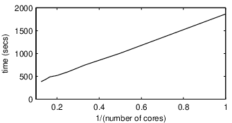
In contrast to Matsuda’s implementation there is no dependency between the calculation of each of the test statistics. On a multicore CPU a test statistic can be assigned to each core, and upon completion the next statistic needing calculation is assigned. Due to the small overheads this introduces, compute-time minus a (near) constant factor for calculating the frequency-averaged periodogram is simply inversely proportional to the number of cores used. The fact that for large most time is spent in calculating the test statistics means that our algorithm can be effectively scaled for higher dimensionality just by using more processor cores. The example of Fig. 7 illustrates the inverse proportionality, using an 8 core processor.

8 Application to EEG Data
We now apply the MHT method to electroencephalogram (EEG) data, (resting conditions with eyes closed), for 33 males, 19 diagnosed with negative-syndrome schizophrenia, and 24 controls. This rare heritage clinical dataset from unmedicated patients was discussed in detail in [15]. Interest is in detecting any differences in patterns of brain connectivity between the groups.


For each individual EEG was recorded on the scalp at sites so that is a vector-valued process. There are possible graph structures, and possible connections between the series (edges to the graph). Each possible connection was assigned a connection index from 1 to 45 as given in [15].
For illustration purposes, the ten channel time series for one of the negative-syndrome patients is shown in Fig. 8. For each of the negative-syndrome patients the MHT algorithm was used to determine whether an index- connection existed, and the percentage of the group of patients exhibiting this connection was recorded. The same was done for the control group. Fig. 9 gives the resulting percentages for each connection and both groups. For 3/4 of the connections the percentage is lower for the controls, suggesting patients exhibit a tendency towards higher connectivity, a result consistent with [15] where completely different methodology was used.
9 Concluding Discussion
Matsuda’s approach to identification of a graphical model involves an appealing Kullback-Leibler statistic but, while improving on exhaustive search approaches, his implementation using a backward stepwise selection is extremely heavy computationally. This paper introduced a multiple hypothesis test implementation using Matsuda’s statistic. The number of statistics needing to be calculated is reduced by and the computational burden for evaluating the test statistics themselves is notably reduced as iterative fitting algorithms are no longer required.
The MHT approach allows us to derive a more relevant control on the error rate in contrast to the stepwise procedure where the error rate used in each test step doesn’t have a clear link to the total error of the procedure. The type I error rate we are controlling is the probability of failing to delete an edge when it is missing in the true graphical model. It may be more intuitive to define the error as deleting an edge that is contained in the true graph. In order to do this we would have to accurately know the distribution of the test statistic under this alternative, which unfortunately we don’t know this.
The conservative nature of the Holm approach can in theory be somewhat offset by using an adaptive approach, (explained in detail by Guo [9]), particularly for large The result is a more powerful test than the standard Holm procedure and although the FWER will be higher, Guo showed it still controls the FWER asymptotically. We implemented this methodology but for our examples and the values of utilised, differences were very small; however, this approach is undoubtedly worthy of further investigation.
It is possible using our method to conduct an efficient stepwise approach by running the MHT and keeping all edges that clearly exist (i.e., have a very large test statistic), thus defining a new to that used previously. Much of the work is thus completed. Then the MHT can be re-run to test models differing from by one edge, but such additional steps require the iterative scheme [22].
Finally, we have shown that the algorithm scales very well — is highly parallelizable — with appropriate computing resources. Future work would involve rendering the algorithm for efficient calculation on high performance computing hardware such as GPUs.
Appendix: Random Model Construction
For our simulations random models were constructed by randomly formulating matrices with the number of zero entries specified as follows.
For a given value a matrix was constructed with null entries. All diagonal elements and non-diagonal elements in position for which were populated by random values sampled from the distribution. The matrix was then subject to spectral decomposition and any eigenvalues with modulus greater than unity were replaced by their reciprocals and reconstructed using the modified eigenvalues. For such a we know [12, pp. 15 & 653] and so a stationary process results. The choice of controls the sparsity; our default choice makes approximately % of the matrix entries zero for
Acknowledgement
The work of Rob Wolstenholme was supported by EPSRC (UK). .
References
- [1] F. R. Bach and M. I. Jordan, “Learning graphical models for stationary time series,” IEEE Trans. Signal Process. vol. 52, pp. 2189–99, 2004.
- [2] D. R. Brillinger, “Remarks concerning graphical models for time series and point processes,” Revista de Econometria (Brazilian Review of Econometrics), vol. 16, pp. 1–23, 1996.
- [3] R. Dahlhaus, “Graphical interaction models for multivariate time series,” Metrika, vol. 51, pp. 157-172, 2000.
- [4] D. M. Edwards, Introduction to Graphical Modelling, 2nd Ed. New York: Springer, 2000.
- [5] M. Eichler, “Fitting graphical interaction models to multivariate time series,” in Proceedings of the Twenty-Second Conference on Uncertainty in Artificial Intelligence. Arlington, VA: AUAI Press, pp. 147–154, 2006.
- [6] M. Fiecas, H. Ombao, C. Linkletter, W. Thompson & J. Sanes, “Functional connectivity: shrinkage estimation and randomization test,” NeuroImage, vol. 49, pp. 3005–3014, 2010.
- [7] R. Fried and V. Didelez, “Decomposability and selection of graphical models for time series,” Biometrika, vol. 90, pp. 251–67, 2003. 251Ð267.
- [8] U. Gather, M. Imhoff and R. Fried, “Graphical models for multivariate time series from intensive care monitoring,” Statist. Med., vol. 21, pp. 2685Ð-701, 2002.
- [9] W. Guo, “A note on adaptive Bonferroni and Holm procedures under dependence,” Biometrika, vol. 96, pp. 1012–1018, 2009.
- [10] D. Kazakos and P. Papantoni-Kazakos, “Spectral distance measures between Gaussian Processes” IEEE Trans. on Automatic Control, vol. 25, pp. 950-59.
- [11] E. L. Lehmann and J. P. Romano, Testing Statistical Hypotheses, 3rd Ed. New York: Springer, 2005.
- [12] H. Lütkepohl, New Introduction to Multiple Time Series Analysis. Berlin: Springer, 2006.
- [13] Y. Matsuda, “A test statistic for graphical modelling of multivariate time series,” Biometrika, vol. 93, pp. 399–409, 2006.
- [14] Y. Matsuda, Y. Yajima & H. Tong, “Selecting models with different spectral density matrix structures by the cross-validated log likelihood criterion,” Bernoulli, vol. 12, pp. 221–249, 2006.
- [15] T. Medkour, A. T. Walden, A. P. Burgess & V. B. Strelets, “Brain connectivity in positive and negative syndrome schizophrenia,” Neuroscience, vol. 169, pp. 1779–88.
- [16] M. B. Priestley, Spectral Analysis and Time Series. London UK: Academic Press, 1981.
- [17] J. P. Shaffer, “Multiple hypothesis testing,” Annual Review of Psychology, vol. 46, pp. 561–584.
- [18] J. Songsiri, J. Dahl & L. Vandenberghe, “Graphical models of autoregressive processes,” in Convex Optimization in Signal Processing and Communications, D. P. Palomar and Y. C. Eldar, Eds. Cambridge UK: Cambridge University Press, 2010.
- [19] J. Songsiri, J. Dahl & L. Vandenberghe, “Topology selection in graphical models of autoregressive processes,” Journal of Machine Learning Research, vol. 11, pp. 2671–2705, 2010.
- [20] T. P. Speed and H. Kiiveri, “Gaussian Markov distributions over finite graphs,” Annals of Statistics, vol. 14, pp. 138–150, 1986.
- [21] J. Timmer, M. Lauk, S. Häußler, V. Radt, B. Köster, B. Hellwig, B. Guschlbauer, C.H. Lücking, M. Eichler and G. Deuschl, “Cross-spectral analysis of tremor time series,” Internat. J. Bifurcation and Chaos, vol. 10, pp. 2595–2610, 2000.
- [22] N. Wermuth and E. Scheidt, “Fitting a covariance selection model to a matrix,” Applied Statistics, vol. 26, pp. 88–92, 1977.
*