跳到论文正文
W Papers独立论文阅读器 arXiv:1502.01920 论文正文 计算阅读时间 · 0%
引用这篇论文根据当前论文元数据生成,正式投稿前建议核对。


License: arXiv.org perpetual non-exclusive license
arXiv:1502.01920v1 [math.DS] 06 Feb 2015

Quantization causes waves:
Smooth finitely computable functions are affine

Vladimir Anashin
Date: August 24, 2026
Abstract.

Given an automaton (a letter-to-letter transducer) 𝔄\mathfrak{A} whose input and output alphabets are 𝔽p={0,1,…,p−1}\mathbb{F}_{p}=\{0,1,\ldots,p-1\}, one visualizes word transformations performed by 𝔄\mathfrak{A} by a point set 𝐏⁡(𝔄)\mathbf{P}(\mathfrak{A}) of real plane ℝ2\mathbb{R}^{2} as follows: To an mm-letter non-empty word v=γm−1​γm−2​…​γ0v=\gamma_{m-1}\gamma_{m-2}\ldots\gamma_{0} over the alphabet 𝒜\mathcal{A} put into the correspondence a rational number 0.v0.v whose base-pp expansion is 0.γm−1​γm−2​…​γ00.\gamma_{m-1}\gamma_{m-2}\ldots\gamma_{0}; then to every mm-letter input word w=αm−1αm−2⋯α0w=\alpha_{m-1}\alpha_{m-2}\cdots\alpha_{0} of the automaton 𝔄\mathfrak{A} and to the respective mm-letter output word 𝔞(w)=βm−1βm−2⋯β0\mathfrak{a}(w)=\beta_{m-1}\beta_{m-2}\cdots\beta_{0} (rightmost letters are feeded to/outputted from the automaton prior to leftmost ones) there corresponds a point (0.w;0.𝔞(w))(0.w;0.{\mathfrak{a}(w)}) of the real unit square [0,1]2[0,1]^{2}; denote 𝐏⁡(𝔄)\mathbf{P}(\mathfrak{A}) a closure (in the topology of ℝ2\mathbb{R}^{2}) of the point set (0.w;0.𝔞(w))(0.w;0.{\mathfrak{a}(w)}) where ww ranges over the set 𝒲\mathcal{W} of all non-empty words over the alphabet 𝔽p\mathbb{F}_{p}.

For a finite-state automaton 𝔄\mathfrak{A}, it is shown that once some points of 𝐏⁡(𝔄)\mathbf{P}(\mathfrak{A}) constitute a smooth (of a class C2C^{2}) curve in ℝ2\mathbb{R}^{2}, the curve is a segment of a straight line with a rational slope; and there are only finitely many straight lines whose segments are in 𝐏⁡(𝔄)\mathbf{P}(\mathfrak{A}). Moreover, when identifying 𝐏⁡(𝔄)\mathbf{P}(\mathfrak{A}) with a subset of a 2-dimensional torus 𝕋2⊂ℝ3\mathbb{T}^{2}\subset\mathbb{R}^{3} (under a natural mapping of the real unit square [0,1]2[0,1]^{2} onto 𝕋2\mathbb{T}^{2}) the smooth curves from 𝐏⁡(𝔄)\mathbf{P}(\mathfrak{A}) constitute a collection of torus windings. In cylindrical coordinates either of the windings can be ascribed to a complex-valued function ψ⁡(x)=ei⁡(A​x−2​π​B​(t))\psi(x)=e^{i(Ax-2\pi B(t))} (x∈ℝ)(x\in\mathbb{R}) for suitable rational A,B⁡(t)A,B(t). Since ψ⁡(x)\psi(x) is a standard expression for a matter wave in quantum theory (where B⁡(t)=t​B​(t0)B(t)=tB(t_{0})), and since transducers can be regarded as a mathematical formalization for causal discrete systems, the main result of the paper might serve as a mathematical reasoning why wave phenomena are inherent in quantum systems: This is because of causality principle and the discreteness of matter.

1. Introduction

In the paper, we examine C2C^{2}-smooth real functions which can be computed (in some new but natural meaning which is rigorously defined below) on finite automata, i.e., on sequential machines that have only finite number of states. We show that all these functions are affine and, moreover, that they can be expressed as complex functions ei⁡(A​x+B)e^{i(Ax+B)} and thus can be ascribed (also in some natural rigorous meaning) to matter waves from quantum theory.

A general problem of evaluation of real functions on abstract discrete machines naturally arose at the very moment the first digital computers had been invented. There are a number of various mathematical statements of the problem which depend both on specific mathematical model of a digital computer (the abstract machine) and on the representation of reals in some ‘digital’ form. For instance, real number computations on Turing machines constitute a core of theory of constructive reals and computable functions. The theory demonstrates intensive development for during more than half a century, see e.g. [36] and references therein. Sequential machines (also known as Mealy automata, or as finite-state letter-to-letter transducers) are, speaking loosely, Turing machines whose heads move only in one direction. Sequential machines are therefore less power computers compared to general Turing machines; however, a number of real world phenomena and processes can be modelled by sequential machines since the latter can be considered as (non-autonomous) discrete dynamical systems. That is why the theory of functions computable by sequential machines, which constitutes a substantial part of automata theory, has numerous applications not only in mathematics itself (e.g., in real analysis, pp-adic analysis, number theory, complexity theory, dynamics, etc.) but also in computer science, physics, linguistics and in many other sciences, see e.g. monographs [2, 3, 8, 9, 15, 29, 47] for details and references.

The paper was motivated by empirical data obtained during a research project related to an applied problem which assumed intensive computer experiments with automata modelling of various cryptographic primitives used in stream ciphers, hash functions, etc. Word transformations performed by the automata where visualised, namely, represented by points of the unit square 𝕀2=[0,1]×[0,1]\mathbb{I}^{2}=[0,1]\times[0,1] in real plane ℝ2\mathbb{R}^{2} so that coordinates of the points relate numerical (radix) representations of input words to the numerical representations of corresponding output words. It was noticed that once the modelled system was finite-state, and once input words were taken sufficiently long, some linear structures (looking like segments of straight lines and somewhat resembling pictures from a double-slit experiment in quantum physics, cf. Figures 4–4 and Figure 14) may appear in the graph, but more complicated structures like smooth curves of higher order had never been observed. A particular aim of the paper is to give mathematical explanation of the phenomenon and to characterize these linear structures.

But during the research it became evident that the problem (which actually is a question what smooth real functions can be modelled on finite automata) has applications not only to cryptography (see e.g. [3, Chapter 11]) but also may be related to mathematical formalism of quantum theory. As a matter of fact, the latter relation (which we believe does exist) can be regarded as a yet another answer to the following question discussed by A. Khrennikov in a series of papers devoted to so-called Prequantum Classical Statistical Field theory, see e.g. [23, 22]: Why mathematical formalism of quantum theory (which is based on the theory of linear operators on Hilbert spaces) is essentially linear although a number of quantum phenomena demonstrate an extremely non-linear behavior?

Thus the goal of the paper is twofold:

  • •

    firstly, to characterize real functions which can be computed by finite automata; and

  • •

    secondly, to give (using obtained description of the functions) some mathematical reasoning why wave phenomena are inherent in quantum systems.

The major part of the paper focuses on real functions which can be computed by finite automata while the said mathematical reasoning is considered in a closing section which contains a discussion of possible applications of mathematical results of the paper to quantum theory. We are not going to discuss cryptographic applications here; they will be postponed to forthcoming papers.

In the paper, by a general automaton (whose set of states is not necessarily finite) we mean a machine which performs letter-by-letter transformations of words over input alphabet into words over output alphabet: Once a letter is feeded to the automaton, the automaton updates its current state (which initially is fixed and so is the same for all input words) to the next one and produces corresponding output letter. Both the next state and the output letter depend both on the current state and on the input letter. Therefore each letter of output word depends only on those letters of input word which have already been feeded to the automaton. An input word is a finite sequence of letters; the letters can naturally be ascribed to ‘causes’ while letters of the corresponding output word can be regarded as ‘effects. ‘Causality’ just means that effects depend only on causes that ‘already have happened’; therefore an automaton is an adequate mathematical formalism for a specific manifestation of causality principle once we assume that there exist only finitely many causes and effects, cf., e.g.,[44, 45].

When studying real functions that can be computed by an automaton 𝔄\mathfrak{A} whose input/output alphabets are 𝒜={0,1,…,p−1}\mathcal{A}=\{0,1,\ldots,p-1\} (where p>1p>1 is an integer from ℕ={1,2,3,…}\mathbb{N}=\{1,2,3,\ldots\}) most authors follow common approach which described in e.g. [15, Chapter XIII, Section 4]: They associate an infinite word α1​α2​…​αn​…\alpha_{1}\alpha_{2}\ldots\alpha_{n}\ldots over 𝒜\mathcal{A} to a real number whose base-pp expansion is 0.α1​α2​…​αn​…=∑i=1∞αi​p−i0.\alpha_{1}\alpha_{2}\ldots\alpha_{n}\ldots=\sum_{i=1}^{\infty}\alpha_{i}p^{-i} and consider a real function d𝔄d_{\mathfrak{A}} defined as follows: Given x∈[0,1]x\in[0,1], take its base-pp expansion x=∑i=1∞αi​p−ix=\sum_{i=1}^{\infty}\alpha_{i}p^{-i}; then produce an infinite output sequence β1​β2​…​βn​…\beta_{1}\beta_{2}\ldots\beta_{n}\ldots of 𝔄\mathfrak{A} by successfully feeding the automaton with the letters α1\alpha_{1}, α2\alpha_{2}, etc., and put d𝔄​(x)=∑i=1∞βi​p−id_{\mathfrak{A}}(x)=\sum_{i=1}^{\infty}\beta_{i}p^{-i}. Being feeded by infinite input sequence α1​α2​…​αn​…\alpha_{1}\alpha_{2}\ldots\alpha_{n}\ldots, the automaton 𝔄\mathfrak{A} produces a unique infinite output sequence β1​β2​…​βn​…\beta_{1}\beta_{2}\ldots\beta_{n}\ldots; therefore the function d𝔄d_{\mathfrak{A}} is well defined everywhere on the real closed unit interval (segment) 𝕀=[0,1]\mathbb{I}=[0,1] with the exception of maybe a countable set D⊂[0,1]D\subset[0,1] of points; namely, of those having two distinct base-pp expansions 0.γ1​γ2​…​γn​0​…​0​…=0.γ1​γ2​…​γn−1​(γn−1)​(p−1)​…​(p−1)​…0.\gamma_{1}\gamma_{2}\ldots\gamma_{n}0\ldots 0\ldots=0.\gamma_{1}\gamma_{2}\ldots\gamma_{n-1}(\gamma_{n}-1)(p-1)\ldots(p-1)\ldots. The point set 𝐌⁡(𝔄)={(x;d𝔄​(x))∈ℝ2:x∈[0,1]}\mathbf{M}(\mathfrak{A})=\{(x;d_{\mathfrak{A}}(x))\in\mathbb{R}^{2}\colon x\in[0,1]\} can be considered as a graph of the real function d𝔄d_{\mathfrak{A}} specified by the automaton 𝔄\mathfrak{A} (every time, before being feeded by the very first letter of each infinite input word the automaton 𝔄\mathfrak{A} is assumed to be in a fixed state s0s_{0}, the initial state). Indeed, d𝔄​(x)d_{\mathfrak{A}}(x) is defined uniquely for x∈[0,1]∖Dx\in[0,1]\setminus D and d𝔄​(x)d_{\mathfrak{A}}(x) can be ascribed to at most two values for x∈Dx\in D; so d𝔄d_{\mathfrak{A}} can be treated a real function which is defined on the unit segment [0,1][0,1] and has not more that a countable number points of discontinuity in [0,1][0,1]. In the sequel we refer 𝐌⁡(𝔄)\mathbf{M}(\mathfrak{A}) as to the Monna graph of the automaton 𝔄\mathfrak{A}, cf. Subsection 2.5.

The said common approach (and its various generalisations) is utilised in numerous papers, see e.g. [10, 11, 27, 28, 39]. Speaking loosely, the common approach looks as if one feeds the automaton 𝔄\mathfrak{A} by a base-pp expansion of a real number x∈[0,1]x\in[0,1] so that leftmost (i.e., the most significant) digits are feeded to the automaton prior to rightmost ones and observes output as real numbers since the automaton outputs accordingly leftmost digits of the base-pp expansion of d𝔄​(x)∈[0,1]d_{\mathfrak{A}}(x)\in[0,1] prior to rightmost ones thus ascribing to the automaton 𝔄\mathfrak{A} the real function d𝔄d_{\mathfrak{A}}. We stress that the function d𝔄d_{\mathfrak{A}} is well defined almost everywhere on [0,1][0,1] due to namely that order in which digits of base-pp expansion are feeded to (and outputted from) the automaton 𝔄\mathfrak{A}.

A crucial difference of the approach used in our paper from the mentioned one is that the order we feed digits to (and read digits from) the automaton is inverse: Namely,

  1. (i)

    given a real number x∈[0,1]x\in[0,1], we represent xx via base-pp expansion x=0.α1​α2​…​αn​…x=0.\alpha_{1}\alpha_{2}\ldots\alpha_{n}\ldots (we take both expansions if xx has two distinct ones);

  2. (ii)

    from the base-pp expansion 0.α1​α2​…​αn​…0.\alpha_{1}\alpha_{2}\ldots\alpha_{n}\ldots we derive corresponding sequence α1,α1​α2,α1​α2​α3,…\alpha_{1},\alpha_{1}\alpha_{2},\alpha_{1}\alpha_{2}\alpha_{3},\ldots of words; then

  3. (iii)

    feeding the automaton 𝔄\mathfrak{A} successively by the words α1,α1​α2,α1​α2​α3,…\alpha_{1},\alpha_{1}\alpha_{2},\alpha_{1}\alpha_{2}\alpha_{3},\ldots so that rightmost letters are feeded to 𝔄\mathfrak{A} prior to leftmost ones we obtain corresponding output word sequence ζ11,ζ12​ζ22,ζ13​ζ23​ζ33,…\zeta_{11},\zeta_{12}\zeta_{22},\zeta_{13}\zeta_{23}\zeta_{33},\ldots;

  4. (iv)

    to the output sequence we put into a correspondence the sequence 𝒮⁡(x)\mathcal{S}(x) of rational numbers whose base-pp expansions are 0.ζ11,0.ζ12​ζ22,0.ζ13​ζ23​ζ33,…0.\zeta_{11},0.\zeta_{12}\zeta_{22},0.\zeta_{13}\zeta_{23}\zeta_{33},\ldots thus obtaining a point set 𝒳(x)={(0.α1…αi;0.ζ1​iζ2​i…ζi​i):i=1,2,…}\mathcal{X}(x)=\{(0.\alpha_{1}\ldots\alpha_{i};0.\zeta_{1i}\zeta_{2i}\ldots\zeta_{ii})\colon i=1,2,\ldots\} in the real unit square 𝕀2=[0,1]×[0,1]\mathbb{I}^{2}=[0,1]\times[0,1]; after that

  5. (v)

    we consider the set ℱ⁡(x)\mathcal{F}(x) of all cluster points of the sequence 𝒮⁡(x)\mathcal{S}(x);

  6. (vi)

    finally, we specify a real plot (or, briefly, a plot) of the automaton 𝔄\mathfrak{A} as a union 𝐏(𝔄)=∪x∈[0,1],y∈ℱ⁡(x)((x;y)∪𝒳(x))\mathbf{P}(\mathfrak{A})=\cup_{x\in[0,1],y\in\mathcal{F}(x)}((x;y)\cup\mathcal{X}(x)).

In other words, 𝐏⁡(𝔄)\mathbf{P}(\mathfrak{A}) is a closure in the unit square 𝕀2\mathbb{I}^{2} of the union ∪i=1∞𝐋i(𝔄)\cup_{i=1}^{\infty}\mathbf{L}_{i}(\mathfrak{A}) where 𝐋i(𝔄)={(0.α1…αi;0.ζ1​iζ2​i…ζi​i):x∈𝕀}\mathbf{L}_{i}(\mathfrak{A})=\{(0.\alpha_{1}\ldots\alpha_{i};0.\zeta_{1i}\zeta_{2i}\ldots\zeta_{ii})\colon x\in\mathbb{I}\} is the ii-th layer of the plot 𝐏⁡(𝔄)\mathbf{P}(\mathfrak{A}). That is, the plot 𝐏⁡(𝔄)\mathbf{P}(\mathfrak{A}) can be considered as a ‘limit’ of the sequence of sets ∪i=1n𝐋i(𝔄)\cup_{i=1}^{n}\mathbf{L}_{i}(\mathfrak{A}), the approximate plots at word length NN, while N→∞N\to\infty (see more formal definitions in Subsection 2.5). Note that according to automata 0-1 law (cf. [3, Proposition 11.15] and [6]) the plot 𝐏⁡(𝔄)\mathbf{P}(\mathfrak{A}) of arbitrary automaton 𝔄\mathfrak{A} can be of two kinds only: Either 𝐏⁡(𝔄)=𝕀2\mathbf{P}(\mathfrak{A})=\mathbb{I}^{2} or 𝐏⁡(𝔄)\mathbf{P}(\mathfrak{A}) is a (Lebesgue) measure-0 closed subset of ℝ2\mathbb{R}^{2}. Moreover, if the number of states of the automaton 𝔄\mathfrak{A} is finite (further in the paper these automata are referred to as finite ones), then the second case takes place.

We stress crucial advantage of real plots over Monna graphs: In a contrast to the Monna graph 𝐌⁡(𝔄)\mathbf{M}(\mathfrak{A}), a real plot 𝐏⁡(𝔄)\mathbf{P}(\mathfrak{A}) is capable of showing true long-term behavior of automaton 𝔄\mathfrak{A} (i.e., when 𝔄\mathfrak{A} is feeded by sufficiently long words) rather than a short-term behaviour displayed by the Monna graph 𝐌⁡(𝔄)\mathbf{M}(\mathfrak{A}) since due to the very construction of the real plot the higher order (i.e., the most significant) digits of the real number represented by the output word are formed by the latest outputted letters of the output word whereas the construction of the Monna graph assumes that the higher order digits are formed by the earliest outputted letters. This results in a drastically different appearances of the real plot and of the Monna graph: Real plot clearly demonstrates that corresponding automaton is ‘ultimately linear’ (that is, exhibits linear long-term behavior), cf. Figures 4–4; whereas the Monna graph is incapable to reveal this important feature of the automaton, cf. Figure 4. This is the main reason why in the paper we focus on real plots of automata rather than on their Monna graphs.

Refer to caption
Figure 1.  Approximate plot of an automaton at word length 16
Refer to caption
Figure 2.  Approximate plot of the same automaton at word length 17
Refer to caption
Figure 3. Cluster points of the plot of the same automaton     
Refer to caption
Figure 4. The Monna graph of the same automaton

Therefore when specifying a notion of computability of a real-valued function g:G→[0,1]g\colon G\rightarrow[0,1] (where G⊂[0,1]G\subset[0,1]) on automata, at least two different approaches do exist: The first one is to speak of the case when the graph 𝐆⁡(g)={(x;g⁡(x)):x∈G}\mathbf{G}(g)=\{(x;g(x))\colon x\in G\} of the function GG lie completely in 𝐌⁡(𝔄)\mathbf{M}(\mathfrak{A}) for some automaton 𝔄\mathfrak{A} while the second one is to consider the case when 𝐆⁡(g)⊂𝐏⁡(𝔄)\mathbf{G}(g)\subset\mathbf{P}(\mathfrak{A}). Papers [10, 11, 27, 28, 39] mentioned above basically deal with the computability in the first meaning whereas our’s paper deals with the computability of the second kind. Note that classes of real functions which are computable on finite automata are different depending on the meaning: For instance, the function ⌊p​x⌋\lfloor px\rfloor (where ⌊a⌋\lfloor a\rfloor stands for the integral part of a∈ℝa\in\mathbb{R}, i.e., for the biggest integer not exceeding aa) is not computable in the first meaning but is computable in the second one whilst the function p−1​xp^{-1}x is computable in the first meaning but is not computable in the second one.

To the best of our knowledge, our approach (which is based on real plots rather than on Monna graphs) was originally used in [3] and was never considered before by other authors.

In the sequel we refer real functions g:G→[0,1]g\colon G\rightarrow[0,1] with domain G⊂[0,1]G\subset[0,1] as to finitely computable if there exists a finite automaton 𝔄\mathfrak{A} whose real plot contains the graph of the function gg; i.e., if 𝐆⁡(g)⊂𝐏⁡(𝔄)\mathbf{G}(g)\subset\mathbf{P}(\mathfrak{A}). Main result of our paper is Theorem 5.1 which characterizes all finitely computable C2C^{2}-functions gg defined on a sub-segment D=[a,b)⊂[0,1]D=[a,b)\subset[0,1]: The theorem yields that if a finitely computable function g:D→[0,1]g\colon D\rightarrow[0,1] is twice differentiable and if its second derivative is continuous everywhere on DD then gg is necessarily affine of the form g⁡(x)=A​x+Bg(x)=Ax+B for suitable rational pp-adic A,BA,B (that is, for AA, BB which can be represented by irreducible fractions whose denominators are co-prime to pp). Moreover, this is true in nn-dimensional case as well (Theorem 5.5).

In view of Theorem 5.1 it is noteworthy that despite the classes of functions computable on finite automata are different depending on the meaning the computability is understood, nonetheless if a function g:[0,1]→[0,1]g\colon[0,1]\rightarrow[0,1] is everywhere differentiable on (0,1)(0,1) and 𝐆⁡(g)⊂𝐌⁡(𝔄)\mathbf{G}(g)\subset\mathbf{M}(\mathfrak{A}) for some finite automaton 𝔄\mathfrak{A} with binary input/output alphabets then gg is necessarily affine, see [28]. In [27] it is shown that a similar assertion holds for multivariate continuously differentiable functions and arbitrary finite alphabets. Therefore finite automata should be judged as rather ‘weak computers’ in all meanings since only quite simple real functions can be evaluated on these devices. From this view, results of the current paper are some contribution to the theory of computable real functions.

It is worth mentioning right now that actually our proof reveals a basic reason why smooth functions which can be represented by finite automata are necessarily affine: This is because squaring can not be performed by a finite automaton; that is, an automaton which, being feeded by a base-pp expansion of nn, outputs a base-pp expansion of n2n^{2} for every positive integer nn, can not be finite (the latter is a well-known fact from automata theory, see e.g., [8, Theorem 2.2.3]).

It is also worth mentioning that the question when 𝐆⁡(g)⊂𝐌⁡(𝔄)\mathbf{G}(g)\subset\mathbf{M}(\mathfrak{A}) is somewhat easier to handle than the question when 𝐆⁡(g)⊂𝐏⁡(𝔄)\mathbf{G}(g)\subset\mathbf{P}(\mathfrak{A}). Indeed, in the first case once the automaton 𝔄\mathfrak{A} is feeded by an infinite word …​α3​α2​α1\ldots\alpha_{3}\alpha_{2}\alpha_{1}, the word is treated as a base-pp expansion of a unique real number x=0.α1​α2​α3​…∈[0,1]x=0.\alpha_{1}\alpha_{2}\alpha_{3}\ldots\in[0,1], corresponding output of 𝔄\mathfrak{A} is also an infinite word …​β3​β2​β1\ldots\beta_{3}\beta_{2}\beta_{1} which also is treated as a base-pp expansion of a unique real number y=0.β1​β2​β3​…∈[0,1]y=0.\beta_{1}\beta_{2}\beta_{3}\ldots\in[0,1]. This results in a unique point (x;y)(x;y) of the unit square 𝕀2\mathbb{I}^{2} in the first case; whilst in the second case the automaton 𝔄\mathfrak{A}, being feeded by the infinite word …​α3​α2​α1\ldots\alpha_{3}\alpha_{2}\alpha_{1}, produces generally an infinite point set of a cardinality continuum: The set is a closure of the point set {(0.αnαn−1…α1;0.βnβn−1…β1):n=1,2,…}\{(0.\alpha_{n}\alpha_{n-1}\ldots\alpha_{1};0.\beta_{n}\beta_{n-1}\ldots\beta_{1})\colon n=1,2,\ldots\} in 𝕀2\mathbb{I}^{2}. Due to this reason during the proofs we have to use more complicated techniques from real analysis which in some cases we combine with methods of pp-adic analysis. Therefore some proofs are involved; but to make general idea of a proof as transparent as possible in the sequel we explain it in loose terms when appropriate.

Last but not least: Our approach reveals another important feature of smooth functions which can be computed on finite automata. From Figure 4 it can be clearly observed that limit points of the plot constitute a torus winding if one converts a unit square into torus by gluing together opposite sides of the square. This is not occasional: Our Theorem 5.1 yields that if the unit square 𝕀2\mathbb{I}^{2} is mapped onto a torus 𝕋2⊂ℝ3\mathbb{T}^{2}\subset\mathbb{R}^{3}, the smooth curves from the plot become torus windings; and these windings after being represented in cylindrical coordinates are described by complex-valued functions ei⁡(A​x+B)e^{i(Ax+B)} (x∈[0,1]x\in[0,1]), see Corollary 3.13. But in quantum theory the latter exponential functions are ascribed to matter waves (cf., de Broglie waves); therefore, since automata can be considered as models for discrete casual systems, the results of our paper give some mathematical evidence that matter waves are inherent in quantum systems merely due to causality principle and discreteness of matter (quantization). We discuss these possible connections to physics in Section 6.

Note that for not to overload the paper with extra calculations we consider only automata whose input and output alphabets consist of pp letters 0,1,…,p−10,1,\ldots,p-1 where p>1p>1 is a prime number though our approach can be expanded to the case when pp is arbitrary integer greater than 1 (and even to the case when pp is not necessarily an integer, see Section 6). For a prime pp, we naturally associate when necessary letters of the alphabet 0,1,…,p−10,1,\ldots,p-1 to residues modulo pp, i.e., to elements of a finite field 𝔽p\mathbb{F}_{p}.

The paper is organized as follows:

  • •

    In Section 2 we recall basic definitions as well as some (mostly known) facts from combinatorics of words, from automata theory, from pp-adic analysis, and from knot theory. Also in this section we formally introduce the notion of real plot of automaton and examine its basic properties.

  • •

    In Section 3 we completely describe cluster points of real plots of finite autonomous automata and of finite affine automata: We show that the points constitute links of torus knots.

  • •

    In Section 4 we prove numerous (mostly technical) results on finitely computable functions; that is, on real functions whose graphs lie in plots of finite automata. Loosely speaking, in the section we (rigorously) develop techniques to examine real functions computed on finite automata as if the automata are feeded by base-pp expansions of real arguments of the functions so that less significant digits are feeded to automaton prior to more significant ones.

  • •

    Section 5 contains main results of the paper: We prove that once a finitely computable function is C2C^{2}-smooth than it is affine and may be associated to a finite collection of complex-valued functions Ψ⁡(x,ℓ)=ei⁡(A​x−2​π​pℓ​B)\Psi(x,\ell)=e^{i(Ax-2\pi p^{\ell}B)}, (x∈ℝ,ℓ∈ℕ0)(x\in\mathbb{R};\ell\in\mathbb{N}_{0}) for suitable rational numbers A,BA,B which are pp-adic integers. We prove a multivariate version of the theorem as well.

  • •

    In Section 6 we discuss possible connections of the main results to informational interpretation of quantum theory. We argue that the results show that wave function is a mathematical consequence of two basic assumptions which are causality principle and discreteness of matter: We show that using β\beta-expansions of real numbers (where β=1+τ\beta=1+\tau and τ>0\tau>0 is small) rather than base-pp expansions for positive integer p>1p>1, main results of the paper imply that a quantum system may be considered as a finite automaton which calculates functions ei⁡(A​x−2​π​βℓ​B)e^{i(Ax-2\pi\beta^{\ell}B)}; but the functions are approximately equal to a⋅ei⁡(A​x−2​π​t​B)a\cdot e^{i(Ax-2\pi tB)} when t=ℓ​τt=\ell\tau since τ\tau is small and thus (1+τ)ℓ≈1+ℓ​τ(1+\tau)^{\ell}\approx 1+\ell\tau; moreover, β=1+τ\beta=1+\tau implies that both input and output alphabets of the automaton must be necessarily binary, i.e., {0,1}\{0,1\}. Therefore one may say that the automaton produces waves a⋅ei⁡(A​x−2​π​t​B)a\cdot e^{i(Ax-2\pi tB)} (since variables x,t∈ℝx,t\in\mathbb{R} may be regarded as ‘position’ and ‘time’ respectively) from bits. This may serve a mathematical evidence in favour of J. A. Wheeler’s It from bit doctrine which suggests that all things physical (‘its’) are information-theoretic in origin (‘from bits’), [46].

2. Preliminaries

Technically the paper is a sort of interplay between real analysis and pp-adic analysis; but although real analysis is the tool we mostly use in proofs, in some important places we also use pp-adic analysis to examine specific properties of automata maps since the maps actually are 1-Lipschitz functions w.r.t. pp-adic metric. This is why we first recall some facts about words over a finite alphabet, pp-adic integers, and automata.

2.1. Few words about words

An alphabet is just a finite non-empty set 𝒜\mathcal{A}; further in the paper usually 𝒜={0,1,…,p−1}=𝔽p\mathcal{A}=\{0,1,\ldots,p-1\}=\mathbb{F}_{p}. Elements of 𝒜\mathcal{A} elements are called symbols, or letters. By the definition, a word of length nn over alphabet 𝒜\mathcal{A} is a finite sequence (stretching from right to left) αn−1⋯α1α0\alpha_{n-1}\cdots\alpha_{1}\alpha_{0}, where αn−1,…,α1,α0∈𝒜\alpha_{n-1},\ldots,\alpha_{1},\alpha_{0}\in\mathcal{A}. The number nn is called the length of the word w=αn−1⋯α1α0w=\alpha_{n-1}\cdots\alpha_{1}\alpha_{0} and is denoted via Λ⁡(w)\Lambda(w). The empty word ϕ\phi is a sequence of length 0, that is, the one that contains no symbols. Given a word w=αn−1⋯α1α0w=\alpha_{n-1}\cdots\alpha_{1}\alpha_{0}, any word v=αk−1⋯α1α0v=\alpha_{k-1}\cdots\alpha_{1}\alpha_{0}, k≤nk\leq n, is called a prefix of the word ww; whereas any word u=αn−1⋯αi+1αiu=\alpha_{n-1}\cdots\alpha_{i+1}\alpha_{i}, 0≤i≤n−10\leq i\leq n-1 is called a suffix of the word ww. Every word αj⋯αi+1αi\alpha_{j}\cdots\alpha_{i+1}\alpha_{i} where n−1≥j≥i≥0n-1\geq j\geq i\geq 0 is called a subword of the word w=αn−1⋯α1α0w=\alpha_{n-1}\cdots\alpha_{1}\alpha_{0}. Given words a=αn−1⋯α1α0a=\alpha_{n-1}\cdots\alpha_{1}\alpha_{0} and b=βk−1⋯β1β0b=\beta_{k-1}\cdots\beta_{1}\beta_{0}, the concatenation a​bab is the following word (of length n+kn+k):

ab=αn−1⋯α1α0βk−1⋯β1β0.ab=\alpha_{n-1}\cdots\alpha_{1}\alpha_{0}\beta_{k-1}\cdots\beta_{1}\beta_{0}.

Given a word ww, its kk-times concatenation is denoted via (w)k(w)^{k}:

(w)k=w​w​…​w⏟k​times.(w)^{k}=\underbrace{ww\ldots w}_{k\ \text{times}}.

We denote via 𝒲\mathcal{W} the set of all non-empty words over 𝒜={0,1,…,p−1}\mathcal{A}=\{0,1,\ldots,p-1\} and via 𝒲ϕ\mathcal{W}_{\phi} the set of all words including the empty word ϕ\phi. In the sequel the set of all nn-letter words over the alphabet 𝔽p\mathbb{F}_{p} we denote as 𝒲n\mathcal{W}_{n}; so 𝒲=∪n=1∞𝒲n\mathcal{W}=\cup_{n=1}^{\infty}\mathcal{W}_{n}. To every word w=αn−1⋯α1α0w=\alpha_{n-1}\cdots\alpha_{1}\alpha_{0} we put into the correspondence a non-negative integer 𝗇𝗎𝗆⁡(w)=α0+α1⋅p+⋯+αn−1⋅pn−1\operatorname{\mathsf{num}}(w)=\alpha_{0}+\alpha_{1}\cdot p+\cdots+\alpha_{n-1}\cdot p^{n-1}. Thus 𝗇𝗎𝗆\operatorname{\mathsf{num}} maps the set 𝒲\mathcal{W} of all non-empty finite words over the alphabet 𝒜\mathcal{A} onto the set ℕ0={0,1,2,…}\mathbb{N}_{0}=\{0,1,2,\ldots\} of all non-negative integers. We will also consider a map ρ\rho of the set 𝒲\mathcal{W} into the real unit half-open interval [0,1)[0,1); the map ρ\rho is defined as follows: Given w=βr−1​…​β0∈𝒲w=\beta_{r-1}\ldots\beta_{0}\in\mathcal{W}, put

ρ⁡(w)=𝗇𝗎𝗆⁡(w)⋅p−Λ⁡(w)=β0+β1​p+⋯+βr−1​pr−1pr=0.βr−1​…​β0∈[0,1).\rho(w)=\operatorname{\mathsf{num}}(w)\cdot p^{-\Lambda(w)}=\frac{\beta_{0}+\beta_{1}p+\cdots+\beta_{r-1}p^{r-1}}{p^{r}}=0.\beta_{r-1}\ldots\beta_{0}\in[0,1). (2.1)

We also use the notation 0.w0.w for 0.βr−1​…​β00.\beta_{r-1}\ldots\beta_{0}.

Along with finite words we also consider (left-)infinite words over the alphabet 𝒜\mathcal{A}; the ones are the infinite sequences of the form …​α2​α1​α0\ldots\alpha_{2}\alpha_{1}\alpha_{0} where αi∈𝒜\alpha_{i}\in\mathcal{A}, i∈ℕ0i\in\mathbb{N}_{0}. For infinite words the notion of a prefix and of a subword are defined in the same way as for finite words; whilst suffix is not defined. Let an infinite word ww be eventually periodic, that is, let w=…​βt−1​βt−2​…​β0​βt−1​βt−2​…​β0​αr−1​αr−2​…​α0w=\ldots\beta_{t-1}\beta_{t-2}\ldots\beta_{0}\beta_{t-1}\beta_{t-2}\ldots\beta_{0}\alpha_{r-1}\alpha_{r-2}\ldots\alpha_{0} for αi​βj∈𝒜\alpha_{i}\beta_{j}\in\mathcal{A}; then the subword βt−1​βt−2​…​β0\beta_{t-1}\beta_{t-2}\ldots\beta_{0} is called a period of the word ww and the suffix αr−2​…​α0\alpha_{r-2}\ldots\alpha_{0} is called the pre-period of the word ww. Note that a pre-period may be an empty word while a period can not. We write the eventually periodic word ww as w=(βt−1​βt−2​…​β0)∞​αr−1​αr−2​…​α0w=(\beta_{t-1}\beta_{t-2}\ldots\beta_{0})^{\infty}\alpha_{r-1}\alpha_{r-2}\ldots\alpha_{0}.

2.2. pp-adic numbers

See [17, 20, 26] for introduction to pp-adic analysis or comprehensive monographs [31, 38] for further reading.

Fix a prime number pp and denote respectively via ℕ={1,2,…}\mathbb{N}=\{1,2,\ldots\} and ℤ={0,±1,±2,…}\mathbb{Z}=\{0,\pm 1,\pm 2,\ldots\} the set of all positive rational integers and the ring of all rational integers. Given n∈ℕ=ℕ0∖{0}n\in\mathbb{N}=\mathbb{N}_{0}\setminus\{0\}, the pp-adic absolute value of nn is |n|p=p−ordp⁡n|n|_{p}=p^{-\operatorname{ord}_{p}n}, where pordp⁡np^{\operatorname{ord}_{p}n} is the largest power of pp which is a factor of nn; so n=n′⋅pordp⁡nn=n^{\prime}\cdot p^{\operatorname{ord}_{p}n} where n′∈ℕn^{\prime}\in\mathbb{N} is co-prime to pp. By putting |0|p=0|0|_{p}=0, |−n|p=|n|p|-n|_{p}=|n|_{p} and |n/m|p=|n|p/|m|p|n/m|_{p}=|n|_{p}/|m|_{p} for n,m∈ℤn,m\in\mathbb{Z}, m≠0m\neq 0 we expand the pp-adic absolute value to the whole field ℚ\mathbb{Q} of rational numbers. Given an absolute value ||p|~|_{p}, we define a metric in a standard way: |a−b|p|a-b|_{p} is a pp-adic metric on ℚ\mathbb{Q}. The field ℚp\mathbb{Q}_{p} of pp-adic numbers is a completion of the field ℚ\mathbb{Q} of rational numbers w.r.t. the pp-adic metric while the ring ℤp\mathbb{Z}_{p} of pp-adic integers is a ring of integers of ℚp\mathbb{Q}_{p}; and the ring ℤp\mathbb{Z}_{p} is a completion of ℤ\mathbb{Z} w.r.t. the pp-adic metric. The ring ℤp\mathbb{Z}_{p} is compact w.r.t. the pp-adic metric: Actually ℤp\mathbb{Z}_{p} is a ball of radius 1 centered at 0; namely ℤp={r∈ℚp:|r|p≤1}\mathbb{Z}_{p}=\{r\in\mathbb{Q}_{p}\colon|r|_{p}\leq 1\}. Balls in ℚp\mathbb{Q}_{p} are clopen; that is, both closed and open w.r.t. the pp-adic metric.

A pp-adic number r∈ℚp∖{0}r\in\mathbb{Q}_{p}\setminus\{0\} admits a unique pp-adic canonical expansion r=∑i=k∞αi​pir=\sum_{i=k}^{\infty}\alpha_{i}p^{i} where αi∈{0,1,…,p−1}\alpha_{i}\in\{0,1,\ldots,p-1\}, k∈ℤk\in\mathbb{Z}, αk≠0\alpha_{k}\neq 0. Note that then any pp-adic integer z∈ℤpz\in\mathbb{Z}_{p} admits a unique representation z=∑i=0∞αi​piz=\sum_{i=0}^{\infty}\alpha_{i}p^{i} for suitable αi∈{0,1,…,p−1}\alpha_{i}\in\{0,1,\ldots,p-1\}. The latter representation is called a canonical form (or, a canonical representation) of the pp-adic integer z∈ℤpz\in\mathbb{Z}_{p}; the ii-th coefficient αi\alpha_{i} of the expansion will be referred to as the ii-th pp-adic digit of zz and denoted via αi=δi​(z)\alpha_{i}=\delta_{i}(z). It is clear that once z∈ℕ0z\in\mathbb{N}_{0}, the ii-th pp-adic digit δi​(z)\delta_{i}(z) of zz is just the ii-th digit in the base-pp expansion of zz. Note also that a pp-adic integer z∈ℤpz\in\mathbb{Z}_{p} is a unity of ℤp\mathbb{Z}_{p} (i.e., has a multiplicative inverse z−1∈ℤpz^{-1}\in\mathbb{Z}_{p}) if and only if δ0​(z)≠0\delta_{0}(z)\neq 0; so any pp-adic number z∈ℚpz\in\mathbb{Q}_{p} has a unique representation of the form z=z′⋅|z|p−1z=z^{\prime}\cdot|z|_{p}^{-1} where z′∈ℤpz^{\prime}\in\mathbb{Z}_{p} is a unity.

The pp-adic integers may be associated to infinite words over the alphabet 𝔽p={0,1,…,p−1}\mathbb{F}_{p}=\{0,1,\ldots,p-1\} as follows: Given a pp-adic integer z∈ℤpz\in\mathbb{Z}_{p}, consider its canonical expansion z=∑i=0∞αi⋅piz=\sum_{i=0}^{\infty}\alpha_{i}\cdot p^{i}; then denote via 𝗐𝗋𝖽⁡(z)\operatorname{\mathsf{wrd}}(z) the infinite word …​α2​α1​α0\ldots\alpha_{2}\alpha_{1}\alpha_{0} (allowing some freedom of saying we will sometimes refer 𝗐𝗋𝖽⁡(z)\operatorname{\mathsf{wrd}}(z) as to a base-pp expansion of z∈ℤpz\in\mathbb{Z}_{p}). Vice versa, given a left-infinite word w=…​α2​α1​α0w=\ldots\alpha_{2}\alpha_{1}\alpha_{0} we denote via 𝗇𝗎𝗆⁡(w)=∑i=0∞αi⋅pi\operatorname{\mathsf{num}}(w)=\sum_{i=0}^{\infty}\alpha_{i}\cdot p^{i} corresponding pp-adic integer whose base-pp expansion is ww thus expanding the mapping 𝗇𝗎𝗆\operatorname{\mathsf{num}} defined in Subsection 2.1 to the case of infinite words as well. It is worth noticing here that addition and multiplication of pp-adic integers can be performed by using the same school-textbook algorithms for addition/multiplication of non-negative integers represented via their base-pp expansions with the only difference: The algorithms are applied to infinite words that correspond to pp-adic canonical forms of summands/multipliers rather than to a finite words which are base-pp expansions of summands/multipliers.

Given n∈ℕn\in\mathbb{N} and a canonical expansion z=∑i=0∞αi​piz=\sum_{i=0}^{\infty}\alpha_{i}p^{i} for z∈ℤpz\in\mathbb{Z}_{p}, denote z𝗆𝗈𝖽pn=∑i=0n−1αi​piz\mathbin{\mathsf{mod}}{p^{n}}=\sum_{i=0}^{n-1}\alpha_{i}p^{i}. The mapping 𝗆𝗈𝖽pn:z↦z𝗆𝗈𝖽pn\mathbin{\mathsf{mod}}{p^{n}}\colon z\mapsto z\mathbin{\mathsf{mod}}{p^{n}} is a ring epimorphism of ℤp\mathbb{Z}_{p} onto the residue ring ℤ/pn​ℤ\mathbb{Z}/p^{n}\mathbb{Z} (under a natural representation of elements of the residue ring by the least non-negative residues {0,1​…,pn−1}\{0,1\ldots,p^{n}-1\}).

The series in the right-hand side of the canonical form converges w.r.t. the pp-adic metric; that is, the sequence of partial sums z𝗆𝗈𝖽pnz\mathbin{\mathsf{mod}}{p^{n}} converges to zz w.r.t. the pp-adic metric: limn→∞p(z𝗆𝗈𝖽pn)=z\lim_{n\to\infty}^{p}(z\mathbin{\mathsf{mod}}p^{n})=z. It is worth noticing here that arbitrary infinite series ∑i=0∞ri\sum_{i=0}^{\infty}r_{i} where ri∈ℚpr_{i}\in\mathbb{Q}_{p} converges in ℚp\mathbb{Q}_{p} (i.e., w.r.t. pp-adic metric) if and only if limi→∞|ri|p=0\lim_{i\to\infty}|r_{i}|_{p}=0 since pp-adic metric is non-Archimedean; that is, it satisfies strong triangle inequality |x−y|p≤max⁡{|x−z|p,|z−y|p}|x-y|_{p}\leq\max\{|x-z|_{p},|z-y|_{p}\} for all x,y,z∈ℚpx,y,z\in\mathbb{Q}_{p}.

Note that z∈ℕ0z\in\mathbb{N}_{0} if and only if all but a finite number of coefficients αi\alpha_{i} in the canonical form are 0 while z∈{−1,−2,−3,…}z\in\{-1,-2,-3,\ldots\} if and only if all but a finite number of αi\alpha_{i} are p−1p-1. Further we will need a special representation for pp-adic integer rationals; that is, for those rational numbers zz which at the same time are pp-adic integers, i.e., for z∈ℤp∩ℚz\in\mathbb{Z}_{p}\cap\mathbb{Q}. Note that z∈ℤp∩ℚz\in\mathbb{Z}_{p}\cap\mathbb{Q} if and only if zz can be represented by an irreducible fraction z=a/bz=a/b, a∈ℤ,b∈ℕa\in\mathbb{Z},b\in\mathbb{N} where bb is co-prime to pp. The following proposition is well known, cf., e.g., [16, Theorem 10]:

Proposition 2.1.

A pp-adic integer zz is rational (i.e., z∈ℤp∩ℚz\in\mathbb{Z}_{p}\cap\mathbb{Q}) if and only if the sequence of coefficients of its canonical form is eventually periodic:

z=α0+α1​p+⋯+αr−1​pr−1+(β0+β1​p+⋯+βt−1​pt−1)​pr+(β0+β1​p+⋯+βt−1​pt−1)​pr+t+(β0+β1​p+⋯+βt−1​pt−1)​pr+2​t+⋯z=\alpha_{0}+\alpha_{1}p+\cdots+\alpha_{r-1}p^{r-1}+(\beta_{0}+\beta_{1}p+\cdots+\beta_{t-1}p^{t-1})p^{r}+\\ (\beta_{0}+\beta_{1}p+\cdots+\beta_{t-1}p^{t-1})p^{r+t}+(\beta_{0}+\beta_{1}p+\cdots+\beta_{t-1}p^{t-1})p^{r+2t}+\cdots (2.2)

for suitable αj,βi∈{0,1,…,p−1}\alpha_{j},\beta_{i}\in\{0,1,\ldots,p-1\}, r∈ℕ0r\in\mathbb{N}_{0}, t∈ℕt\in\mathbb{N} (the sum α0+α1​p+⋯+αr−1​pr−1\alpha_{0}+\alpha_{1}p+\cdots+\alpha_{r-1}p^{r-1} is absent in the above expression once r=0r=0).

In other words, once a pp-adic integer zz is represented in its canonical form, z=∑i+0∞γi​piz=\sum_{i+0}^{\infty}\gamma_{i}p^{i}, the corresponding infinite word …​γ1​γ0\ldots\gamma_{1}\gamma_{0} is eventually periodic: …​γ1​γ0=(βt−1​…​β0)∞​αr−1​…​α0\ldots\gamma_{1}\gamma_{0}=(\beta_{t-1}\ldots\beta_{0})^{\infty}\alpha_{r-1}\ldots\alpha_{0}. It is clear that given z∈ℤp∩ℚz\in\mathbb{Z}_{p}\cap\mathbb{Q}, both rr and tt are not unique: For instance,

(βt−1​…​β0)∞​αr−1​…​α0=(β0​βt−1​…​β1​β0​βt−1​…​β1)∞​αr​αr−1​…​α0,(\beta_{t-1}\ldots\beta_{0})^{\infty}\alpha_{r-1}\ldots\alpha_{0}=(\beta_{0}\beta_{t-1}\ldots\beta_{1}\beta_{0}\beta_{t-1}\ldots\beta_{1})^{\infty}\alpha_{r}\alpha_{r-1}\ldots\alpha_{0},

where αr=β0\alpha_{r}=\beta_{0}. But once both pre-periodic and periodic parts (the prefix αr−1​…​α0\alpha_{r-1}\ldots\alpha_{0} and the word βt−1​…​β0\beta_{t-1}\ldots\beta_{0} ) are taken the shortest possible, both the pre-period length rr and the period length tt are unique for a given pp-adic rational integer z∈ℤp∩ℚz\in\mathbb{Z}_{p}\cap\mathbb{Q}; we refer to αr−1​…​α0\alpha_{r-1}\ldots\alpha_{0} and to βt−1​βt−2​…​β1​β0\beta_{t-1}\beta_{t-2}\ldots\beta_{1}\beta_{0} as to pre-period of zz and period of zz accordingly.

Given z∈ℤp∩ℚz\in\mathbb{Z}_{p}\cap\mathbb{Q} we mostly assume further that in the representation z=α0+⋯+αr−1​pr−1+(β0+⋯+βt−1​pt−1)⋅∑j=0∞pr+t​jz=\alpha_{0}+\cdots+\alpha_{r-1}p^{r-1}+(\beta_{0}+\cdots+\beta_{t-1}p^{t-1})\cdot\sum_{j=0}^{\infty}p^{r+tj} (respectively, in eventually periodic infinite word 𝗐𝗋𝖽⁡(z)=(βt−1​…​β0)∞​αr−1​…​α0\operatorname{\mathsf{wrd}}(z)=(\beta_{t-1}\ldots\beta_{0})^{\infty}\alpha_{r-1}\ldots\alpha_{0} that corresponds to zz) rr is a pre-period length and tt is a period length. Note that a pre-period may be an empty word (i.e., of length 0) while a period can not.

Rational pp-adic integers can also be represented as fractions of a special kind:

Proposition 2.2.

A pp-adic integer z∈ℤpz\in\mathbb{Z}_{p} is rational if and only if there exist t∈ℕt\in\mathbb{N}, c∈ℤc\in\mathbb{Z}, d∈{0,1,…,pt−2}d\in\{0,1,\ldots,p^{t}-2\} such that

z=c+dpt−1.z=c+\frac{d}{p^{t}-1}. (2.3)
Proof.

Indeed, z∈ℤp∩ℚz\in\mathbb{Z}_{p}\cap\mathbb{Q} if and only if zz is of the form (2.2); therefore

z=(α0+α1​p+⋯+αr−1​pr−1−pr)+pr​(1−β0+β1​p+⋯+βt−1​pt−1pt−1)=(α0+α1​p+⋯+αr−1​pr−1−pr+q)+ζ0+ζ1​p+⋯+ζt−1​pt−1pt−1z=(\alpha_{0}+\alpha_{1}p+\cdots+\alpha_{r-1}p^{r-1}-p^{r})+p^{r}\left(1-\frac{\beta_{0}+\beta_{1}p+\cdots+\beta_{t-1}p^{t-1}}{p^{t}-1}\right)=\\ (\alpha_{0}+\alpha_{1}p+\cdots+\alpha_{r-1}p^{r-1}-p^{r}+q)+\frac{\zeta_{0}+\zeta_{1}p+\cdots+\zeta_{t-1}p^{t-1}}{p^{t}-1} (2.4)

where ζ0+ζ1​p+⋯+ζt−1​pt−1\zeta_{0}+\zeta_{1}p+\cdots+\zeta_{t-1}p^{t-1} is a base-pp expansion of the least non-negative residue ss of pr​(pt−1−(β0+β1​p+⋯+βt−1​pt−1))=(pt−1)​q+sp^{r}(p^{t}-1-(\beta_{0}+\beta_{1}p+\cdots+\beta_{t-1}p^{t-1}))=(p^{t}-1)q+s modulo pt−1p^{t}-1. ∎

Note 2.3.

Recall that (1−pm)−1=∑i=0∞pm​i∈ℤp(1-p^{m})^{-1}=\sum_{i=0}^{\infty}p^{mi}\in\mathbb{Z}_{p}, for every m∈ℕm\in\mathbb{N}.

Note 2.4.

Note that once in (2.4) rr is a pre-period length and tt is a period length of z∈ℤp∩ℚz\in\mathbb{Z}_{p}\cap\mathbb{Q}, the representation (2.3) is unique; that is, the choice of cc and dd in (2.3) is unique.

In the sequel we often use base-pp expansions of pp-adic rational integers reduced modulo 1 (recall that if y∈ℝy\in\mathbb{R} then by the definition y𝗆𝗈𝖽1=y−⌊y⌋∈[0,1)⊂ℝy\mathbin{\mathsf{mod}}1=y-\lfloor y\rfloor\in[0,1)\subset\mathbb{R}) along with their pp-adic canonical forms. For reader’s convenience, we now summarize some facts on connections between these representations.

It is very well known that a base-pp expansion of a rational number is eventually periodic; that is, given x∈ℚ∩[0,1]x\in\mathbb{Q}\cap[0,1], the base-pp expansion for xx is

x=0.χ0​…​χk−1​(ξ0​…​ξn−1)∞=χ0​p−1+χ1​p−2+⋯+χk−1​p−k+ξ0​p−k−1+ξ1​p−k−2+⋯+ξn−1​p−k−n+ξ0​p−k−1−n+ξ1​p−k−2−n+⋯+ξn−1​p−k−2​n+⋯=1pk​(χ0​pk−1+χ1​pk−2+⋯+χk−1)+1pk⋅ξ0​pn−1+ξ1​pn−2+⋯+ξn−1pn−1,x=0.\chi_{0}\ldots\chi_{k-1}(\xi_{0}\ldots\xi_{n-1})^{\infty}=\\ \chi_{0}p^{-1}+\chi_{1}p^{-2}+\cdots+\chi_{k-1}p^{-k}+\xi_{0}p^{-k-1}+\xi_{1}p^{-k-2}+\cdots+\xi_{n-1}p^{-k-n}+\\ \xi_{0}p^{-k-1-n}+\xi_{1}p^{-k-2-n}+\cdots+\xi_{n-1}p^{-k-2n}+\cdots=\\ \frac{1}{p^{k}}(\chi_{0}p^{k-1}+\chi_{1}p^{k-2}+\cdots+\chi_{k-1})+\frac{1}{p^{k}}\cdot\frac{\xi_{0}p^{n-1}+\xi_{1}p^{n-2}+\cdots+\xi_{n-1}}{p^{n}-1}, (2.5)

where χi,ξj∈{0,1,…,p−1}\chi_{i},\xi_{j}\in\{0,1,\ldots,p-1\}. Note that in the base-pp expansions of rational integers from [0,1][0,1] we use right-infinite words rather than left-infinite ones that correspond to canonical expansions of pp-adic integers.

Proposition 2.5.

Given z∈ℤp∩ℚz\in\mathbb{Z}_{p}\cap\mathbb{Q}, represent zz in the form (2.2); then

z𝗆𝗈𝖽1=0.(β^t−1−r¯​β^t−2−r¯​…​β^0​β^t−1​β^t−2​…​β^t−r¯)∞𝗆𝗈𝖽1,z\mathbin{\mathsf{mod}}1=0.(\hat{\beta}_{t-1-\bar{r}}\hat{\beta}_{t-2-\bar{r}}\ldots\hat{\beta}_{0}\hat{\beta}_{t-1}\hat{\beta}_{t-2}\ldots\hat{\beta}_{t-\bar{r}})^{\infty}\mathbin{\mathsf{mod}}1,

where β^=p−1−β\hat{\beta}=p-1-\beta for β∈{0,1,…,p−1}\beta\in\{0,1,\ldots,p-1\} and r¯\bar{r} is the least non-negative residue of rr modulo tt if t>1t>1 or r¯=0\bar{r}=0 if otherwise.

Proof.

Indeed, by Note 2.3, ∑j=0∞pr+t​j=−pr​(pt−1)−1\sum_{j=0}^{\infty}p^{r+tj}=-p^{r}(p^{t}-1)^{-1} in ℤp\mathbb{Z}_{p}; so z=u−v​pr​(pt−1)−1z=u-vp^{r}(p^{t}-1)^{-1} where u=α0+α1​p+⋯+αr−1​pr−1u=\alpha_{0}+\alpha_{1}p+\cdots+\alpha_{r-1}p^{r-1} and v=β0+β1​p+⋯+βt−1​pt−1v=\beta_{0}+\beta_{1}p+\cdots+\beta_{t-1}p^{t-1}. Therefore

z𝗆𝗈𝖽1=(−v​prpt−1)𝗆𝗈𝖽1.z\mathbin{\mathsf{mod}}1=\left(-\frac{vp^{r}}{p^{t}-1}\right)\mathbin{\mathsf{mod}}1.

But (pt−1)−1=p−t+p−2​t+p−3​t+⋯(p^{t}-1)^{-1}=p^{-t}+p^{-2t}+p^{-3t}+\cdots in ℝ\mathbb{R}; so

(pt−1)−1=0.(00​…​0⏟t−1​1)∞(p^{t}-1)^{-1}=0.(\underbrace{00\ldots 0}_{t-1}1)^{\infty}

and thus −v⋅(pt−1)−1=−0.(βt−1βt−2…β0)∞-v\cdot(p^{t}-1)^{-1}=-0.(\beta_{t-1}\beta_{t-2}\ldots\beta_{0})^{\infty}.

Now just note that

(p−1−γ0)+(p−1−γ1)​p+⋯+(p−1−γs−1)​ps−1=ps−1−(γ0+γ1​p+⋯+γs−1​ps−1)(p-1-\gamma_{0})+(p-1-\gamma_{1})p+\cdots+(p-1-\gamma_{s-1})p^{s-1}=p^{s}-1-(\gamma_{0}+\gamma_{1}p+\cdots+\gamma_{s-1}p^{s-1})

for γ0,γ1,…∈{0,1,…,p−1}\gamma_{0},\gamma_{1},\ldots\in\{0,1,\ldots,p-1\}, s∈ℕs\in\mathbb{N}; so

(p−1−γ0)+(p−1−γ1)​p+⋯+(p−1−γs−1)​ps−1ps−1=1−γ0+γ1​p+⋯+γs−1​ps−1ps−1\frac{(p-1-\gamma_{0})+(p-1-\gamma_{1})p+\cdots+(p-1-\gamma_{s-1})p^{s-1}}{p^{s}-1}=\\ 1-\frac{\gamma_{0}+\gamma_{1}p+\cdots+\gamma_{s-1}p^{s-1}}{p^{s}-1}

and therefore

(−0.(γs−1γs−2…γ0)∞)𝗆𝗈𝖽1=(0.(γ^s−1γ^s−2…γ^0)∞)𝗆𝗈𝖽1(-0.(\gamma_{s-1}\gamma_{s-2}\ldots\gamma_{0})^{\infty})\mathbin{\mathsf{mod}}1=(0.(\hat{\gamma}_{s-1}\hat{\gamma}_{s-2}\ldots\hat{\gamma}_{0})^{\infty})\mathbin{\mathsf{mod}}1 (2.6)

where γ^=p−1−γ\hat{\gamma}=p-1-\gamma for γ∈{0,1,…,p−1}\gamma\in\{0,1,\ldots,p-1\}. ∎

Combining (2.5) with Proposition 2.2 we see that all real numbers whose base-pp expansions are purely periodic must lie in ℤp∩ℚ\mathbb{Z}_{p}\cap\mathbb{Q}; therefore the following criterion is true:

Corollary 2.6.

A real number xx is in ℤp∩ℚ\mathbb{Z}_{p}\cap\mathbb{Q} if and only if base-pp expansion of x𝗆𝗈𝖽1x\mathbin{\mathsf{mod}}1 is purely periodic: x𝗆𝗈𝖽1=0.(χ0​…​χn−1)∞x\mathbin{\mathsf{mod}}1=0.(\chi_{0}\ldots\chi_{n-1})^{\infty} for suitable χ0,…,χn−1∈𝔽p\chi_{0},\ldots,\chi_{n-1}\in\mathbb{F}_{p}.

The following corollary expresses base-pp expansion of a pp-adic rational integer via its representation in the form given by Proposition 2.2:

Corollary 2.7.

Once a pp-adic rational integer z∈ℤp∩ℚz\in\mathbb{Z}_{p}\cap\mathbb{Q} is represented in the form as of Proposition 2.2 then z𝗆𝗈𝖽1=0.(ζt−1​ζt−2​…​ζ0)∞z\mathbin{\mathsf{mod}}1=0.(\zeta_{t-1}\zeta_{t-2}\ldots\zeta_{0})^{\infty} where d=ζ0+ζ1​p+⋯+ζt−1​pt−1d=\zeta_{0}+\zeta_{1}p+\cdots+\zeta_{t-1}p^{t-1}.

Proof.

Indeed, under notation of Proposition 2.2, z𝗆𝗈𝖽1=(d⋅(pt−1)−1)𝗆𝗈𝖽1z\mathbin{\mathsf{mod}}1=(d\cdot(p^{t}-1)^{-1})\mathbin{\mathsf{mod}}1 and the result follows since (pt−1)−1=p−t+p−2​t+p−3​t+⋯(p^{t}-1)^{-1}=p^{-t}+p^{-2t}+p^{-3t}+\cdots in ℝ\mathbb{R}. ∎

Now we can find a period length of z∈ℤp∩ℚz\in\mathbb{Z}_{p}\cap\mathbb{Q} provided zz is represented as an irreducible fraction z=a/bz=a/b, where a∈ℤa\in\mathbb{Z}, b∈ℕb\in\mathbb{N}.

Proposition 2.8.

Once a pp-adic rational integer z≠0z\neq 0 is represented as an irreducible fraction z=a/bz=a/b, and if b>1b>1, then the period length tt of zz is equal to the multiplicative order of pp modulo bb (i.e., to the smallest ℓ∈ℕ\ell\in\mathbb{N} such that pℓ≡1(modb)p^{\ell}\equiv 1\pmod{b}).

Proof.

Note that the multiplicative order ℓ\ell of pp modulo bb is the smallest positive integer such that pℓ​(a/b)≡a/b(mod1)p^{\ell}(a/b)\equiv a/b\pmod{1}. Indeed, pℓ=e​b+1p^{\ell}=eb+1 for a suitable e∈ℤe\in\mathbb{Z}; so pℓ​(a/b)=e​a+(a/b)p^{\ell}(a/b)=ea+(a/b). On the other hand, if ps​(a/b)=m+(a/b)p^{s}(a/b)=m+(a/b) for some m∈ℤm\in\mathbb{Z} then a⁡(ps−1)=m​ba(p^{s}-1)=mb and thus ps−1≡0(modb)p^{s}-1\equiv 0\pmod{b} since aa is co-prime to bb (as the fraction a/ba/b is supposed to be irreducible).

Now, from Corollary 2.7 it immediately follows that (pt​z)𝗆𝗈𝖽1=z𝗆𝗈𝖽1(p^{t}z)\mathbin{\mathsf{mod}}1=z\mathbin{\mathsf{mod}}1 once tt is a period length of zz and that tt is the smallest positive integer with that property. Finally we conclude that ℓ=t\ell=t. ∎

Now given b∈ℕb\in\mathbb{N}, bb co-prime to pp, we denote via multb⁡p\operatorname{mult}_{b}p the multiplicative order of pp modulo bb if b>1b>1 or put multb⁡p=1\operatorname{mult}_{b}p=1 once b=1b=1. Then multb⁡p\operatorname{mult}_{b}p is the period length of z∈ℤp∩ℚz\in\mathbb{Z}_{p}\cap\mathbb{Q} once zz is represented as an irreducible fraction z=a/bz=a/b where a∈ℤa\in\mathbb{Z} and b∈ℕb\in\mathbb{N}. Note that we consider here only infinite words that correspond to pp-adic rational integers; thus to, e.g., 0 there corresponds a word (0)∞(0)^{\infty} (so a period of 0 is 0 and a pre-period is empty) and the respective base-pp expansion of 0 is 0.(0)∞0.(0)^{\infty}. Also, 1=1+0⋅p+0⋅p2+⋯1=1+0\cdot p+0\cdot p^{2}+\cdots, the corresponding infinite word is (0)∞​1(0)^{\infty}1; therefore 11 is a pre-period of 1, 00 is a period of 1, and the representation of 1 in the form (2.3) is 1=1+(0/p−1)1=1+(0/p-1).

Example 2.9.

Let p=2p=2; then 1/3=1⋅1+1⋅2+0⋅4+1⋅8+0⋅16+⋯=1−2⋅3−11/3=1\cdot 1+1\cdot 2+0\cdot 4+1\cdot 8+0\cdot 16+\cdots=1-2\cdot 3^{-1} is a canonical 2-adic expansion of 1/31/3; so the corresponding infinite binary word is (01)∞​1(01)^{\infty}1. Therefore the period length of 1/31/3 is 2 (and note that the multiplicative order of 22 modulo 33 is indeed 22), the period is 0101, the pre-period is 11. Also, c=0c=0 and d=1d=1 once 1/31/3 is represented in the form of Proposition 2.2; 1/3=0.(01)∞1/3=0.(01)^{\infty} is a base-2 expansion of 1/31/3, cf. Proposition 2.5 and Corollary 2.7.

2.3. Automata: Basics

Here we remind some basic facts from automata theory (see e.g. monographs [8, 9, 15]).

By the definition, a (non-initial) automaton is a 5-tuple 𝔄=⟨ℐ,𝒮,𝒪,S,O⟩\mathfrak{A}=\langle\mathcal{I},\mathcal{S},\mathcal{O},S,O\rangle where ℐ\mathcal{I} is a finite set, the input alphabet; 𝒪\mathcal{O} is a finite set, the output alphabet; 𝒮\mathcal{S} is a non-empty (possibly, infinite) set of states; S:ℐ×𝒮→𝒮S\colon\mathcal{I}\times\mathcal{S}\to\mathcal{S} is a state transition function; O:ℐ×𝒮→𝒪O\colon\mathcal{I}\times\mathcal{S}\to\mathcal{O} is an output function. An automaton where both input alphabet ℐ\mathcal{I} and output alphabet 𝒪\mathcal{O} are non-empty is called a transducer, see e.g. [2, 9]. The initial automaton 𝔄⁡(s0)=⟨ℐ,𝒮,𝒪,S,O,s0⟩\mathfrak{A}(s_{0})=\langle\mathcal{I},\mathcal{S},\mathcal{O},S,O,s_{0}\rangle is an automaton 𝔄\mathfrak{A} where one state s0∈𝒮s_{0}\in\mathcal{S} is fixed; it is called the initial state. We stress that the definition of an initial automaton 𝔄⁡(s0)\mathfrak{A}(s_{0}) is nearly the same as the one of Mealy automaton (see e.g. [8, 9]) with the only important difference: the set of states 𝒮\mathcal{S} of 𝔄⁡(s0)\mathfrak{A}(s_{0}) is not necessarily finite. Note also that in literature the automata we consider in the paper are also referred to as (letter-to-letter) transducers; in the sequel we use terms ‘automaton’ and ‘transducer’ as synonyms.

Given an input word w=χn−1⋯χ1χ0w=\chi_{n-1}\cdots\chi_{1}\chi_{0} over the alphabet ℐ\mathcal{I}, an initial transducer 𝔄⁡(s0)=⟨ℐ,𝒮,𝒪,S,O,s0⟩\mathfrak{A}(s_{0})=\langle\mathcal{I},\mathcal{S},\mathcal{O},S,O,s_{0}\rangle transforms ww to output word w′=ξn−1⋯ξ1ξ0w^{\prime}=\xi_{n-1}\cdots\xi_{1}\xi_{0} over the output alphabet 𝒪\mathcal{O} as follows (cf. Figure 5): Initially the transducer 𝔄⁡(s0)\mathfrak{A}(s_{0}) is at the state s0s_{0}; accepting the input symbol χ0∈ℐ\chi_{0}\in\mathcal{I}, the transducer outputs the symbol ξ0=O⁡(χ0,so)∈𝒪\xi_{0}=O(\chi_{0},s_{o})\in\mathcal{O} and reaches the state s1=S⁡(χ0,s0)∈𝒮s_{1}=S(\chi_{0},s_{0})\in\mathcal{S}; then the transducer accepts the next input symbol χ1∈ℐ\chi_{1}\in\mathcal{I}, reaches the state s2=S⁡(χ1,s1)∈𝒮s_{2}=S(\chi_{1},s_{1})\in\mathcal{S}, outputs ξ1=O⁡(χ1,s1)∈𝒪\xi_{1}=O(\chi_{1},s_{1})\in\mathcal{O}, and the routine repeats. This way the transducer 𝔄=𝔄⁡(s0)\mathfrak{A}=\mathfrak{A}(s_{0}) defines a mapping 𝔞=𝔞s0\mathfrak{a}=\mathfrak{a}_{s_{0}} of the set 𝒲n​(ℐ)\mathcal{W}_{n}(\mathcal{I}) of all nn-letter words over the input alphabet ℐ\mathcal{I} to the set 𝒲n​(𝒪)\mathcal{W}_{n}(\mathcal{O}) of all nn-letter words over the output alphabet 𝒪\mathcal{O}; thus 𝔄\mathfrak{A} defines a map of the set 𝒲⁡(ℐ)\mathcal{W}(\mathcal{I}) of all non-empty words over the alphabet ℐ\mathcal{I} to the set 𝒲⁡(𝒪)\mathcal{W}(\mathcal{O}) of all non-empty words over the alphabet 𝒪\mathcal{O}. We will denote the latter map by the same symbol 𝔞\mathfrak{a} (or by 𝔞s0\mathfrak{a}_{s_{0}} if we want to stress what initial state is meant), and when it is clear from the context what alphabet 𝒜\mathcal{A} is meant we use notation 𝒲\mathcal{W} rather than 𝒲⁡(𝒜)\mathcal{W}(\mathcal{A}).

1,2.5)(20,13)

Figure 5. Initial transducer, schematically

Throughout the paper, ‘automaton’ mostly stands for ‘initial automaton’; we make corresponding remarks if not. Further in the paper we mostly consider transducers. Furthermore, throughout the paper we consider reachable transducers only; that is, we assume that all states of the initial transducer 𝔄⁡(s0)\mathfrak{A}(s_{0}) are reachable from the initial state s0s_{0}: Given s∈𝒮s\in\mathcal{S}, there exists input word ww over alphabet ℐ\mathcal{I} such that after the word ww has been feeded to the automaton 𝔄⁡(s0)\mathfrak{A}(s_{0}), the automaton reaches the state ss. A reachable transducer is called finite if its set 𝒮\mathcal{S} of states is finite, and transducer is called infinite if otherwise.

To the initial automaton 𝔄⁡(s0)\mathfrak{A}(s_{0}) we put into a correspondence a family ℱ⁡(𝔄)\mathcal{F}(\mathfrak{A}) of all sub-automata 𝔄⁡(s)=⟨ℐ,𝒮~,𝒪,S~,O~,s⟩\mathfrak{A}(s)=\langle\mathcal{I},\tilde{\mathcal{S}},\mathcal{O},\tilde{S},\tilde{O},s\rangle, s∈𝒮s\in\mathcal{S}, where 𝒮~=𝒮~​(s)⊂𝒮\tilde{\mathcal{S}}=\tilde{\mathcal{S}}(s)\subset\mathcal{S} is the set of all states that are reachable from the state ss and S~,O~\tilde{S},\tilde{O} are respective restrictions of the state transition and output functions S,OS,O on ℐ×𝒮~\mathcal{I}\times\tilde{\mathcal{S}}. A sub-automaton 𝔄⁡(s)\mathfrak{A}(s) is called proper if the set 𝒮~\tilde{\mathcal{S}} of all its states is a proper subset of 𝒮\mathcal{S}. A sub-automaton 𝔄⁡(s)\mathfrak{A}(s) is called minimal if it contains no proper sub-automata. It is obvious that a finite sub-automaton is minimal if and only if every its state is reachable from any other its state. The set of all states of a minimal sub-automaton of the automaton 𝔄\mathfrak{A} is called an ergodic component of the (set of all states) of the automaton 𝔄\mathfrak{A}. It is clear that once the automaton is in a state that belongs to an ergodic component, all its further states will also be in the same ergodic component. Therefore all states of a finite automaton are of two types only: The transient states which belong to no ergodic component, and ergodic states which belong to ergodic components. It is clear that the set of all ergodic states is a disjoint union of ergodic components. Note that we use the term ‘minimal automaton’ in a different meaning compared to the one used in automata theory, see, e.g., [15]: Our terminology here is from the theory of Markov chains, see, e.g., [21] (since to the graph of state transitions of every automaton there corresponds a Markov chain).

Hereinafter in the paper the word ‘automaton’ stands for a letter-to-letter initial transducer whose input and output alphabet consists of pp symbols, and we mostly assume that pp is a prime. Thus, for every n=1,2,3,…n=1,2,3,\ldots the automaton 𝔄⁡(s0)=⟨𝔽p,𝒮,𝔽p,S,O,s0⟩\mathfrak{A}(s_{0})=\langle\mathbb{F}_{p},\mathcal{S},\mathbb{F}_{p},S,O,s_{0}\rangle maps nn-letter words over 𝔽p\mathbb{F}_{p} to nn-letter words over 𝔽p\mathbb{F}_{p} according to the procedure described above, cf. Figure 5. Given two such automata 𝔄=𝔄⁡(s0)\mathfrak{A}=\mathfrak{A}(s_{0}) and 𝔅=𝔅⁡(t0)\mathfrak{B}=\mathfrak{B}(t_{0}), their sequential composition (or briefly, a composition) ℭ=𝔅∘𝔄\mathfrak{C}=\mathfrak{B}\circ\mathfrak{A} can be defined in a natural way via sending output of the automaton 𝔄\mathfrak{A} to input of the automaton 𝔅\mathfrak{B} so that the mapping 𝔠:𝒲→𝒲\mathfrak{c}\colon\mathcal{W}\to\mathcal{W} the automaton ℭ\mathfrak{C} performs is just a composite mapping 𝔟∘𝔞\mathfrak{b}\circ\mathfrak{a} (cf. any of monographs [8, 9, 15] for exact definition and further facts mentioned in the subsection). Note that a composition of finite automata is a finite automaton.

In a similar manner one can consider automata with multiply inputs/outputs; these can be also treated as automata whose input/output alphabets are Cartesian powers of 𝔽p\mathbb{F}_{p}: For instance, and automaton with mm inputs and nn outputs over alphabet 𝔽p\mathbb{F}_{p} can be considered as an automaton with a single input over the alphabet 𝔽pm\mathbb{F}_{p}^{m} and a single output over the alphabet 𝔽pn\mathbb{F}_{p}^{n}. Moreover, as the letters of the alphabet 𝔽pk\mathbb{F}_{p}^{k} are in a one-to-one correspondence with residues modulo pkp^{k}; the automaton with mm inputs and nn outputs can be considered (if necessary) as an automaton with a single input over the alphabet ℤ/pm​ℤ\mathbb{Z}/p^{m}\mathbb{Z} and a single output over alphabet ℤ/pn​ℤ\mathbb{Z}/p^{n}\mathbb{Z}.

is an automaton with 2 inputs and 1 output which

Compositions of automata with multiple inputs/outputs can also be naturally defined: For instance, given automata 𝔄1\mathfrak{A}_{1}, 𝔄2\mathfrak{A}_{2}, and 𝔄3\mathfrak{A}_{3} with m1,m2,m3m_{1},m_{2},m_{3} inputs and n1,n2,n3n_{1},n_{2},n_{3} outputs respectively, in the case when m3=n1+n2m_{3}=n_{1}+n_{2} one can consider a composition of these automata by connecting every output of automata 𝔄1\mathfrak{A}_{1} and 𝔄2\mathfrak{A}_{2} to some input of the automaton 𝔄3\mathfrak{A}_{3} so that every input of the automaton 𝔄3\mathfrak{A}_{3} is connected to a unique output which belongs either to 𝔄1\mathfrak{A}_{1} or to 𝔄2\mathfrak{A}_{2} but not to the both. This way one obtains various compositions of automata 𝔄1\mathfrak{A}_{1} and 𝔄2\mathfrak{A}_{2}, with the automaton 𝔄3\mathfrak{A}_{3}, and either of these compositions is an automaton with m1+m2m_{1}+m_{2} inputs and n3n_{3} outputs. Moreover, either of the compositions is a finite automaton if all three automata 𝔄1\mathfrak{A}_{1}, 𝔄2\mathfrak{A}_{2}, 𝔄3\mathfrak{A}_{3} are finite.

Automata can be considered as (generally) non-autonomous dynamical systems on different configuration spaces (e.g., 𝒲n\mathcal{W}_{n}, 𝒲\mathcal{W}, etc.); the system is autonomous when neither the state transition function 𝒮\mathcal{S} nor the output function 𝒪\mathcal{O} depend on input; in this case the automaton is called autonomous as well. For purposes of the paper it is convenient to consider automata with input/output alphabets 𝒜=𝔽p\mathcal{A}=\mathbb{F}_{p} as dynamical systems on the space ℤp\mathbb{Z}_{p} of pp-adic integers, i.e., to relate an automaton 𝔄\mathfrak{A} to a special map f𝔄:ℤp→ℤpf_{\mathfrak{A}}\colon\mathbb{Z}_{p}\to\mathbb{Z}_{p}. In the next subsection we recall some facts about the map f𝔄f_{\mathfrak{A}}.

2.4. Automata maps: the pp-adic view

We identify nn-letter words over 𝔽p\mathbb{F}_{p} with non-negative integers in a natural way: Given an nn-letter word w=χn−1χn−2⋯χ0w=\chi_{n-1}\chi_{n-2}\cdots\chi_{0} (i.e., χi∈𝔽p\chi_{i}\in\mathbb{F}_{p} for i=0,1,2,…,n−1i=0,1,2,\ldots,n-1), we consider ww as a base-pp expansion of the number 𝗇𝗎𝗆⁡(w)=χ0+χ1⋅p+⋯+χn−1⋅pn−1∈ℕ0\operatorname{\mathsf{num}}(w)=\chi_{0}+\chi_{1}\cdot p+\cdots+\chi_{n-1}\cdot p^{n-1}\in\mathbb{N}_{0}. In turn, the latter number can be considered as an element of the residue ring ℤ/pn​ℤ\mathbb{Z}/p^{n}\mathbb{Z} modulo pnp^{n}. We denote via 𝗐𝗋𝖽n\operatorname{\mathsf{wrd}}_{n} an inverse mapping to 𝗇𝗎𝗆\operatorname{\mathsf{num}}. The mapping 𝗐𝗋𝖽n\operatorname{\mathsf{wrd}}_{n} is a bijection of the set {0,1​…,pn−1}⊂ℕ0\{0,1\ldots,p^{n}-1\}\subset\mathbb{N}_{0} onto the set 𝒲n\mathcal{W}_{n} of all nn-letter words over 𝔽p\mathbb{F}_{p}.

As the set {0,1​…,pn−1}\{0,1\ldots,p^{n}-1\} is the set of all non-negative residues modulo pnp^{n} , to every automaton 𝔄=𝔄⁡(s)\mathfrak{A}=\mathfrak{A}(s) there corresponds a map fn,𝔄f_{n,\mathfrak{A}} from ℤ/pn​ℤ\mathbb{Z}/p^{n}\mathbb{Z} to ℤ/pn​ℤ\mathbb{Z}/p^{n}\mathbb{Z}, for every n=1,2,3,…n=1,2,3,\ldots. Namely, for r∈ℤ/pn​ℤr\in\mathbb{Z}/p^{n}\mathbb{Z} put fn,𝔄​(r)=𝗇𝗎𝗆⁡(𝔞⁡(𝗐𝗋𝖽n⁡(r)))f_{n,\mathfrak{A}}(r)=\mathfrak{\operatorname{\mathsf{num}}}(\mathfrak{a}(\operatorname{\mathsf{wrd}}_{n}(r))), where 𝔞\mathfrak{a} is a word transformation of 𝒲n\mathcal{W}_{n} performed by the automaton 𝔄\mathfrak{A}, cf. Subsection 2.3.

Speaking less formally, the mapping fn,𝔄f_{n,\mathfrak{A}} can be defined as follows: given r∈{0,1,…,pn−1}r\in\{0,1,\ldots,p^{n}-1\}, consider a base-pp expansion of rr, read it as a nn-letter word over 𝔽p={0,1,…,p−1}\mathbb{F}_{p}=\{0,1,\ldots,p-1\} (put additional zeroes on higher order positions if necessary) and then feed the word to the automaton so that letters that are on lower order positions (‘less significant digits’) are feeded prior to ones on higher order positions (‘more significant digits’). Then read the corresponding output nn-letter word as a base-pp expansion of a number from ℕ0\mathbb{N}_{0} keeping the same order, i.e. when the earliest outputted letters correspond to lowest order digits in the base-pp expansion.

We stress the following determinative property of the mapping fn,𝔄f_{n,\mathfrak{A}} which follows directly from the definition: Given a,b∈{0,1,…,pn−1}a,b\in\{0,1,\ldots,p^{n}-1\}, whenever a≡b(modpk)a\equiv b\pmod{p^{k}} for some k∈ℕk\in\mathbb{N} then necessarily fn,𝔄​(a)≡fn,𝔄​(b)(modpk)f_{n,\mathfrak{A}}(a)\equiv f_{n,\mathfrak{A}}(b)\pmod{p^{k}}. This implication may be re-stated in terms of pp-adic metric as follows:

|fn,𝔄​(a)−fn,𝔄​(b)|p≤|a−b|p.|f_{n,\mathfrak{A}}(a)-f_{n,\mathfrak{A}}(b)|_{p}\leq|a-b|_{p}. (2.7)

Furthermost, every automaton 𝔄=𝔄⁡(s0)\mathfrak{A}=\mathfrak{A}(s_{0}) defines a mapping f𝔄f_{\mathfrak{A}} from ℤp\mathbb{Z}_{p} to ℤp\mathbb{Z}_{p} which can be specified in a manner similar to the one of the mapping fn,𝔄f_{n,\mathfrak{A}}: Given an infinite word w=…χn−1χn−2⋯χ0w=\ldots\chi_{n-1}\chi_{n-2}\cdots\chi_{0} (that is, an infinite sequence) over 𝔽p\mathbb{F}_{p} we consider a pp-adic integer whose pp-adic canonical expansion is z=z⁡(w)=χ0+χ1⋅p+⋯+χn−1⋅pn−1+⋯z=z(w)=\chi_{0}+\chi_{1}\cdot p+\cdots+\chi_{n-1}\cdot p^{n-1}+\cdots; so, by the definition, for every z∈ℤpz\in\mathbb{Z}_{p} we put

δi​(f𝔄​(z))=O⁡(δi​(z),si)(i=0,1,2,…),\delta_{i}(f_{\mathfrak{A}}(z))=O(\delta_{i}(z),s_{i})\qquad(i=0,1,2,\ldots), (2.8)

where si=S⁡(δi−1​(z),si−1)s_{i}=S(\delta_{i-1}(z),s_{i-1}), i=1,2,…i=1,2,\ldots, and δi​(z)\delta_{i}(z) is the ii-th pp-adic digit of zz; that is, the ii-th term coefficient in the pp-adic canonical representation of zz: δi​(z)=χi∈𝔽p\delta_{i}(z)=\chi_{i}\in\mathbb{F}_{p}, i=0,1,2,…i=0,1,2,\ldots (see Subsection 2.2). The so defined map f𝔄f_{\mathfrak{A}} is called the automaton function (or, the automaton map) of the automaton 𝔄\mathfrak{A}. Note that from (2.8) it follows that

δi​(f𝔄​(z))=Φi​(δ0​(z),…,δi​(z)),\delta_{i}(f_{\mathfrak{A}}(z))=\Phi_{i}(\delta_{0}(z),\ldots,\delta_{i}(z)), (2.9)

where Φi\Phi_{i} is a map from the (i+1)(i+1)-th Cartesian power 𝔽pi+1\mathbb{F}_{p}^{i+1} of 𝔽p\mathbb{F}_{p} into 𝔽p\mathbb{F}_{p}.

More formally, given z∈ℤpz\in\mathbb{Z}_{p}, define f𝔄​(z)f_{\mathfrak{A}}(z) as follows: Consider a sequence (z𝗆𝗈𝖽pn)n=1∞(z\mathbin{\mathsf{mod}}p^{n})_{n=1}^{\infty} and a corresponding sequence (fn,𝔄​(z𝗆𝗈𝖽pn))n=1∞(f_{n,\mathfrak{A}}(z\mathbin{\mathsf{mod}}p^{n}))_{n=1}^{\infty}; then, as the sequence (z𝗆𝗈𝖽pn)n=1∞(z\mathbin{\mathsf{mod}}p^{n})_{n=1}^{\infty} converges to zz w.r.t. pp-adic metric (cf. Subsection 2.2), the sequence (fn,𝔄​(z𝗆𝗈𝖽pn))n=1∞(f_{n,\mathfrak{A}}(z\mathbin{\mathsf{mod}}p^{n}))_{n=1}^{\infty} in view (2.7) also converges w.r.t. the pp-adic metric (since the latter sequence is fundamental and ℤp\mathbb{Z}_{p} is closed in ℚp\mathbb{Q}_{p} which is a complete metric space). Now we just put f𝔄​(z)f_{\mathfrak{A}}(z) to be a limit point of the sequence (fn,𝔄​(z𝗆𝗈𝖽pn))n=1∞(f_{n,\mathfrak{A}}(z\mathbin{\mathsf{mod}}p^{n}))_{n=1}^{\infty}. Thus, the mapping f𝔄f_{\mathfrak{A}} is a well-defined function with domain ℤp\mathbb{Z}_{p} and values in ℤp\mathbb{Z}_{p}; by (2.7) the function f𝔄f_{\mathfrak{A}} satisfies Lipschitz condition with a constant 1 w.r.t. pp-adic metric.

The point is that the class of all automata functions that correspond to automata with pp-letter input/output alphabets coincides with the class of all maps from ℤp\mathbb{Z}_{p} to ℤp\mathbb{Z}_{p} that satisfy the pp-adic Lipschitz condition with a constant 1 (the 1-Lipschitz maps, for brevity), cf., e.g., [5]. We note that the claim can also be derived from a more general result on asynchronous automata [18, Proposition 3.7]; for p=2p=2 the claim was proved in [43].

Further we need more detailed information about finite automata functions, that is, about functions f𝔄:ℤp→ℤpf_{\mathfrak{A}}\colon\mathbb{Z}_{p}\rightarrow\mathbb{Z}_{p} where 𝔄=𝔄⁡(s0)\mathfrak{A}=\mathfrak{A}(s_{0}) is a finite automaton (i.e., with a finite set 𝒮\mathcal{S} of states). It is well known (cf. previous subsection 2.3) that the class of finite automata functions is closed w.r.t. composition of functions and a sum of functions: Once f,g:ℤp→ℤpf,g\colon\mathbb{Z}_{p}\rightarrow\mathbb{Z}_{p} are finite automata functions, either of mappings x↦f⁡(g⁡(x))x\mapsto f(g(x)) and x↦f⁡(x)+g⁡(x)x\mapsto f(x)+g(x) (x∈ℤp)(x\in\mathbb{Z}_{p}) is a finite automaton function. Another important property of finite automata functions is that any finite automaton function maps ℤp∩ℚ\mathbb{Z}_{p}\cap\mathbb{Q} into itself. In view of (2.2), the latter property is just a re-statement of a a well-known property of finite automata which yields that any finite automaton feeded by an eventually periodic sequence outputs an eventually periodic sequence, cf., e.g., [8, Corollary 2.6.9], [15, Chapter XIII, Theorem 2.2.]. Since further we often use that property of finite automata, we state it as a lemma for future references:

Lemma 2.10.

If a finite automaton 𝔄\mathfrak{A} is being feeded by a left-infinite periodic word w∞w^{\infty}, where w∈𝒲w\in\mathcal{W} is a finite non-empty word, then the corresponding output left-infinite word is eventually periodic; i.e., it is of the form u∞​vu^{\infty}v, where u∈𝒲u\in\mathcal{W}, v∈𝒲ϕv\in\mathcal{W}_{\phi}. To put it in other words, if a finite automaton is being feeded by an eventually periodic finite word (w)k​t(w)^{k}t, where w∈𝒲w\in\mathcal{W}, t∈𝒲ϕt\in\mathcal{W}_{\phi}, and k∈ℕk\in\mathbb{N} is sufficiently large, then the output word is of the form r​(u)ℓ​vr(u)^{\ell}v, where ℓ∈ℕ\ell\in\mathbb{N}, u∈𝒲u\in\mathcal{W}, r,v∈𝒲ϕr,v\in\mathcal{W}_{\phi} and rr is either empty or a prefix of uu: u=h​ru=hr for a suitable h∈𝒲ϕh\in\mathcal{W}_{\phi}. Therefore the output word is of the form (u¯)ℓ​v′(\bar{u})^{\ell}v^{\prime}, where u¯\bar{u} is a cyclically shifted word uu.

To study finite automata functions it is convenient sometimes to represent 1-Lipschitz maps from ℤp\mathbb{Z}_{p} to ℤp\mathbb{Z}_{p} as special convergent pp-adic series, the van der Put series. Details about the latter series may be found in, e.g., [31, 38]; here we only briefly recall some basic facts. Given a continuous function f:ℤp→ℤpf\colon\mathbb{Z}_{p}\rightarrow\mathbb{Z}_{p}, there exists a unique sequence B0,B1,B2,…B_{0},B_{1},B_{2},\ldots of pp-adic integers such that

f⁡(z)=∑m=0∞Bm​χ​(m,z)f(z)=\sum_{m=0}^{\infty}B_{m}\chi(m,z) (2.10)

for all z∈ℤpz\in\mathbb{Z}_{p}, where

χ⁡(m,z)={1,if​|z−m|p≤p−n0,otherwise\chi(m,z)=\left\{\begin{array}[]{cl}1,&\text{if}\ \left|z-m\right|_{p}\leq p^{-n}\\ 0,&\text{otherwise}\end{array}\right.

and n=1n=1 if m=0m=0; nn is uniquely defined by the inequality pn−1≤m≤pn−1p^{n-1}\leq m\leq p^{n}-1 otherwise. The right side series in (2.10) is called the van der Put series of the function ff. Note that the sequence B0,B1,…,Bm,…B_{0},B_{1},\ldots,B_{m},\ldots of van der Put coefficients of the function ff tends pp-adically to 00 as m→∞m\to\infty, and the series converges uniformly on ℤp\mathbb{Z}_{p}. Vice versa, if a sequence B0,B1,…,Bm,…B_{0},B_{1},\ldots,B_{m},\ldots of pp-adic integers tends pp-adically to 00 as m→∞m\to\infty, then the the series in the right part of (2.10) converges uniformly on ℤp\mathbb{Z}_{p} and thus define a continuous function f:ℤp→ℤpf\colon\mathbb{Z}_{p}\to\mathbb{Z}_{p}.

The number nn in the definition of χ⁡(m,z)\chi(m,z) has a very natural meaning; it is just the number of digits in a base-pp expansion of m∈ℕ0m\in\mathbb{N}_{0}:

⌊logp⁡m⌋=(the number of digits in a base-​p​expansion for​m)−1;\left\lfloor\log_{p}m\right\rfloor=\left(\text{the number of digits in a base-}p\;\text{expansion for}\;m\right)-1;

therefore n=⌊logp⁡m⌋+1n=\left\lfloor\log_{p}m\right\rfloor+1 for all m∈ℕ0m\in\mathbb{N}_{0} (that is why we assume ⌊logp⁡0⌋=0\left\lfloor\log_{p}0\right\rfloor=0).

Note that coefficients BmB_{m} are related to the values of the function ff in the following way: Let m=m0+…+mn−2​pn−2+mn−1​pn−1m=m_{0}+\ldots+m_{n-2}p^{n-2}+m_{n-1}p^{n-1} be a base-pp expansion for mm, i.e., mj∈{0,…,p−1}m_{j}\in\left\{0,\ldots,p-1\right\}, j=0,1,…,n−1j=0,1,\ldots,n-1 and mn−1≠0m_{n-1}\neq 0, then

Bm={f⁡(m)−f⁡(m−mn−1​pn−1),if​m≥p;f⁡(m),if otherwise.B_{m}=\begin{cases}f(m)-f(m-m_{n-1}p^{n-1}),\ &\text{if}\ m\geq p;\\ f(m),\ &\text{if otherwise}.\par\end{cases} (2.11)

It worth noticing also that χ⁡(m,z)\chi(m,z) is merely a characteristic function of the ball 𝐁p−⌊logp⁡m⌋−1​(m)=m+p⌊logp⁡m⌋−1​ℤp\mathbf{B}_{p^{-\left\lfloor\log_{p}m\right\rfloor-1}}(m)=m+p^{\left\lfloor\log_{p}m\right\rfloor-1}\mathbb{Z}_{p} of radius p−⌊logp⁡m⌋−1p^{-\left\lfloor\log_{p}m\right\rfloor-1} centered at m∈ℕ0m\in\mathbb{N}_{0}:

χ⁡(m,z)={1,if​z≡m(modp⌊logp⁡m⌋+1);0,if otherwise={1,if​x∈𝐁p−⌊logp⁡m⌋−1​(m);0,if otherwise\chi(m,z)=\begin{cases}1,\ &\text{if}\ z\equiv m\pmod{p^{\left\lfloor\log_{p}m\right\rfloor+1}};\\ 0,\ &\text{if otherwise}\par\end{cases}=\begin{cases}1,\ &\text{if}\ x\in\mathbf{B}_{p^{-\left\lfloor\log_{p}m\right\rfloor-1}}(m);\\ 0,\ &\text{if otherwise}\par\end{cases} (2.12)
Theorem 2.11 (cf. [4]).

A function f:ℤp→ℤpf\colon\mathbb{Z}_{p}\rightarrow\mathbb{Z}_{p} is 1-Lipschitz (that is, an automaton function) if and only if ff can be represented as

f⁡(z)=∑m=0∞bm​p⌊logp⁡m⌋​χ​(m,z),f(z)=\sum_{m=0}^{\infty}b_{m}p^{\left\lfloor\log_{p}m\right\rfloor}\chi(m,z), (2.13)

where bm∈ℤpb_{m}\in\mathbb{Z}_{p} for m=0,1,2,…m=0,1,2,\ldots

By using the van der Put series it is possible to determine whether a mapping f:ℤp→ℤpf\colon\mathbb{Z}_{p}\rightarrow\mathbb{Z}_{p} is an automaton function of a finite automaton. We first remind some notions and facts from the theory of automata sequences following [2].

An infinite sequence 𝐚=(ai)i=0∞\mathbf{a}=(a_{i})_{i=0}^{\infty} over a finite alphabet 𝒜\mathcal{A}, #​𝒜=L<∞\#\mathcal{A}=L<\infty, is called pp-automatic if there exists a finite transducer 𝔗=⟨𝔽p,𝒮,𝒜,S,O,s0⟩\mathfrak{T}=\langle\mathbb{F}_{p},\mathcal{S},\mathcal{A},S,O,s_{0}\rangle such that for all n=0,1,2,…n=0,1,2,\ldots, if 𝔗\mathfrak{T} is feeded by the word χkχk−1⋯χ0\chi_{k}\chi_{k-1}\cdots\chi_{0} which is a base-pp expansion of n=χ0+χ1p+⋯χkpkn=\chi_{0}+\chi_{1}p+\cdots\chi_{k}p^{k}, χk≠0\chi_{k}\neq 0 if n≠0n\neq 0, then the kk-th output symbol of 𝔗\mathfrak{T} is ana_{n}; or, in other words, such that δk𝒜​(f𝔗​(n))=an\delta_{k}^{\mathcal{A}}(f_{\mathfrak{T}}(n))=a_{n} for all n∈ℕ0n\in\mathbb{N}_{0}, where k=⌊logp⁡n⌋k=\lfloor\log_{p}n\rfloor and δk𝒜​(r)\delta_{k}^{\mathcal{A}}(r) stands for the kk-th digit in the base-LL expansion of r∈ℕ0r\in\mathbb{N}_{0}.

A pp-kernel of the sequence 𝐚\mathbf{a} is a set kerp⁡(𝐚)\ker_{p}(\mathbf{a}) of all subsequences (aj​pm+t)j=0∞(a_{jp^{m}+t})_{j=0}^{\infty}, m=0,1,2,…m=0,1,2,\ldots, 0≤t<pm0\leq t<p^{m}.

Theorem 2.12 (Automaticity criterion, cf. [2, Theorem 6.6.2]).

A sequence 𝐚\mathbf{a} is pp-automatic if and only if its pp-kernel is finite.

Theorem 2.13 (Finiteness criterion, cf. [5]).

Let a 1-Lipschitz function f:ℤp→ℤpf\colon\mathbb{Z}_{p}\rightarrow\mathbb{Z}_{p} be represented by van der Put series (2.13). The function ff is a finite automaton function if and only if the following conditions hold simultaneously:

  1. (i)

    all coefficients bmb_{m}, m=0,1,2,…m=0,1,2,\ldots, constitute a finite subset Bf⊂ℚ∩ℤpB_{f}\subset\mathbb{Q}\cap\mathbb{Z}_{p}, and

  2. (ii)

    the pp-kernel of the sequence (bm)m=0∞(b_{m})_{m=0}^{\infty} is finite.

Note 2.14.

Condition (ii) of the theorem is equivalent to the condition that the sequence (bm)m=0∞(b_{m})_{m=0}^{\infty} is pp-automatic, cf. Theorem 2.12.

Criteria to determine if an automaton function is finite which are based on expansions other than van der Put are also known, cf. [41, 44].

In literature, automata with multiple inputs and outputs over the same alphabet are also studied. We remark that in the case when the alphabet is 𝔽p\mathbb{F}_{p}, the automata can be considered as automata whose input/output alphabets are Cartesian powers 𝔽pn\mathbb{F}_{p}^{n} and 𝔽pm\mathbb{F}_{p}^{m}, for suitable m,n∈ℕm,n\in\mathbb{N}. For these automata a theory similar to that of automata with a single input/output can be developed: Corresponding automata function are then 1-Lipshitz mappings from ℤpn\mathbb{Z}_{p}^{n} to ℤpm\mathbb{Z}_{p}^{m} w.r.t. pp-adic metrics. Recall that pp-adic absolute value on ℤpk\mathbb{Z}_{p}^{k} is defined as follows: Given (z1,…,zk)∈ℤpk(z_{1},\ldots,z_{k})\in\mathbb{Z}_{p}^{k}, put |(z1,…,zk)|p=max{|zi|p:i=1,2,…,k}|(z_{1},\ldots,z_{k})|_{p}=\max\{|z_{i}|_{p}\colon i=1,2,\ldots,k\}. The so defined absolute value (and the corresponding metric) are non-Archimedean as well. The main theorem of the paper holds (after a proper re-statement) for these automata as well, see Theorem 5.5.

It is worth recalling here a well-known fact (which also can be proved by using Theorem 2.13) that addition of two pp-adic integers can be performed by a finite automaton with two inputs and one output: Actually the automaton just finds successively (digit after digit) the sum by a standard addition-with-carry algorithm which is used to find a sum of two non-negative integers represented by base-pp expansions thus calculating the sum with arbitrarily high accuracy w.r.t. the pp-adic metric. On the contrary, no finite automaton can perform multiplication of two arbitrary pp-adic integers since it is well known that no finite automaton can calculate a base-pp expansion of a square of an arbitrary non-negative integer given a base-pp expansion of the latter, cf., e.g., [8, Theorem 2.2.3].

From these remarks combined with Theorem 2.13 the following properties of finite automata functions can be deduced:

Proposition 2.15.

Let 𝔄,𝔅\mathfrak{A},\mathfrak{B} be finite automata, let a,b∈ℤp∩ℚa,b\in\mathbb{Z}_{p}\cap\mathbb{Q} be pp-adic rational integers. Then the following is true:

  1. (i)

    the mapping z↦f𝔄​(z)+f𝔅​(z)z\mapsto f_{\mathfrak{A}}(z)+f_{\mathfrak{B}}(z) of ℤp\mathbb{Z}_{p} into ℤp\mathbb{Z}_{p} is a finite automaton function;

  2. (ii)

    a composite function f⁡(z)=a⋅f𝔄​(z)+bf(z)=a\cdot f_{\mathfrak{A}}(z)+b, (z∈ℤp)(z\in\mathbb{Z}_{p}), is a finite automaton function;

  3. (iii)

    a constant function f⁡(z)=cf(z)=c is a finite automaton function if and only if c∈ℤp∩ℚc\in\mathbb{Z}_{p}\cap\mathbb{Q};

  4. (iv)

    an affine mapping f⁡(z)=c⋅z+df(z)=c\cdot z+d is a finite automaton function if and only if c,d∈ℤp∩ℚc,d\in\mathbb{Z}_{p}\cap\mathbb{Q}.

Proof.

Note that the van der Put expansion of the constant function z↦cz\mapsto c is

c=c​χ​(0,z)+c​χ​(1,z)+⋯+c​χ​(p−1,z)+0​χ​(p,z)+0​χ​(p+1,z)+⋯,c=c\chi(0,z)+c\chi(1,z)+\cdots+c\chi(p-1,z)+0\chi(p,z)+0\chi(p+1,z)+\cdots, (2.14)

while the van der Put expansion for the identity function z↦zz\mapsto z is

z=∑i=0∞δ⌊logp⁡i⌋​(i)​p⌊logp⁡i⌋​χ​(i,z),z=\sum_{i=0}^{\infty}\delta_{\lfloor\log_{p}i\rfloor}(i)p^{\lfloor\log_{p}i\rfloor}\chi(i,z), (2.15)

where δj​(i)\delta_{j}(i) stands for the jj-th digit in the base-pp expansion of ii. Now all statements of the proposition follow immediately from Theorem 2.13 and the above mentioned facts from finite automata theory. ∎

Note that the statement of Proposition 2.15 is known: For instance, it can be deduced from the old work [30] of A. G. Lunts. To our best knowledge, Lunts was the first who revealed connections between automata theory and pp-adic analysis. It is worth noticing that Lunts defines automata functions in a slightly different way than we do: In his work, an automaton function is a 1-Lipschitz function F:ℚp→ℚpF\colon\mathbb{Q}_{p}\rightarrow\mathbb{Q}_{p} such that F⁡(p​z)=p​F​(z)F(pz)=pF(z) for all z∈ℚpz\in\mathbb{Q}_{p}. Also, Lunts’ methods of proofs are completely different form the ones of Proposition 2.15. Unfortunately, most automata theorists seem to be unaware of the paper [30] since it was never translated into English and even was never reviewed by Mathematical Reviews.

Concluding the subsection, we remark that in literature (finite) automata functions are also known under names of (bounded) determinate functions, or (bounded) deterministic functions, cf., e.g., [47, 10, 11, 41].

2.5. Real plots of automata functions vs Monna graphs.

Further in the paper we consider special representation of automata functions by point sets of real and complex spaces. As we have already mentioned in previous section, several representations of this sort were considered: Via the so-called limit sets (see e.g. [7]), via the Monna graphs (see e.g. [10, 11, 27, 28, 39] ) and via real plots which were originally introduced in [3, Chapter 11]. In the paper we focus on real plots; however we will start this subsection with saying few words about Monna graphs since in some meaning they are counterpart of real plots; and we will not touch limit sets at all since they are standing somewhat apart.

The Monna graphs are based on the Monna’s representation of pp-adic integers via real numbers of the unit closed segment [0,1][0,1] originally suggested by Monna in [34]: Given a canonical expansion z=∑i=0∞αi​piz=\sum_{i=0}^{\infty}\alpha_{i}p^{i} of pp-adic integer z∈ℤpz\in\mathbb{Z}_{p} (cf. Subsection 2.2), consider a real number 𝗆𝗈𝗇⁡(z)=∑i=0∞αi​p−i−1∈[0,1]⊂ℝ\operatorname{\mathsf{mon}}(z)=\sum_{i=0}^{\infty}\alpha_{i}p^{-i-1}\in[0,1]\subset\mathbb{R}. It is clear that 𝗆𝗈𝗇\operatorname{\mathsf{mon}} maps ℤp\mathbb{Z}_{p} onto [0,1][0,1], however, 𝗆𝗈𝗇\operatorname{\mathsf{mon}} is not bijective: The only points from the open interval (0,1)(0,1) that have more than one (actually, exactly two) pre-image w.r.t. 𝗆𝗈𝗇\operatorname{\mathsf{mon}} are rational numbers of the form ∑i=0∞αi​p−i−1\sum_{i=0}^{\infty}\alpha_{i}p^{-i-1} where αi=p−1\alpha_{i}=p-1 for some i≥i0i\geq i_{0} since

∑i=0∞αi​p−i−1=∑i=0∞βi​p−i−1,where\displaystyle\sum_{i=0}^{\infty}\alpha_{i}p^{-i-1}=\sum_{i=0}^{\infty}\beta_{i}p^{-i-1},\ \text{where} (2.16)
βj={αj,if​j≤i0−2;(αi0−1+1)𝗆𝗈𝖽p,if​j=i0;0,if​j≥i0+1\displaystyle\beta_{j}=\begin{cases}\alpha_{j},&\text{if}\ j\leq i_{0}-2;\\ (\alpha_{i_{0}-1}+1)\mathbin{\mathsf{mod}}p,&\text{if}\ j=i_{0};\\ 0,&\text{if}\ j\geq i_{0}+1\end{cases}

where αj=βj\alpha_{j}=\beta_{j} for all j≤i0−2j\leq i_{0}-2, βj=0\beta_{j}=0 for all j≥i0j\geq i_{0} and βi0−1=(αi0−1+1)𝗆𝗈𝖽p\beta_{i_{0}-1}=(\alpha_{i_{0}-1}+1)\mathbin{\mathsf{mod}}p. We can naturally associate the segment [0,1][0,1] (or a half-open interval [0,1)[0,1)) to the real circle 𝕊\mathbb{S} by reducing [0,1][0,1] modulo 1; that is, by taking fractional parts of reals from [0,1][0,1]: 𝕊=[0,1]𝗆𝗈𝖽1\mathbb{S}=[0,1]\mathbin{\mathsf{mod}}1. Then in a similar manner we may consider a mapping of ℤp\mathbb{Z}_{p} onto 𝕊\mathbb{S}; we will denote the mapping also via 𝗆𝗈𝗇\operatorname{\mathsf{mon}} since there is no risk of misunderstanding. Note that w.r.t. the latter mapping the point 0=1∈𝕊0=1\in\mathbb{S} has exactly two pre-images since ∑i=0∞0⋅p−i−1=0=1=∑i=0∞(p−1)⋅p−i−1\sum_{i=0}^{\infty}0\cdot p^{-i-1}=0=1=\sum_{i=0}^{\infty}(p-1)\cdot p^{-i-1} in 𝕊\mathbb{S}.

Now, given an automaton 𝔄=𝔄⁡(s0)\mathfrak{A}=\mathfrak{A}(s_{0}), we define the Monna graph of 𝔄\mathfrak{A} as follows: Let f=f𝔄f=f_{\mathfrak{A}} be a corresponding automaton function, cf. Subsection 2.4 (that is, f:ℤp→ℤpf\colon\mathbb{Z}_{p}\rightarrow\mathbb{Z}_{p} is a 1-Lipschitz function w.r.t. pp-adic metric). Then the Monna graph 𝐌⁡(𝔄)=𝐌⁡(f)\mathbf{M}(\mathfrak{A})=\mathbf{M}(f) (or, which is the same, of the automaton function ff) is the point set 𝐌⁡(𝔄)=𝐌⁡(f)={(𝗆𝗈𝗇⁡(z),𝗆𝗈𝗇⁡(f⁡(z))):z∈ℤp}\mathbf{M}(\mathfrak{A})=\mathbf{M}(f)=\{(\operatorname{\mathsf{mon}}(z),\operatorname{\mathsf{mon}}(f(z)))\colon z\in\mathbb{Z}_{p}\}. Note that we can consider the Monna graph when convenient either as a subset of the unit real square 𝕀2\mathbb{I}^{2}, a Cartesian square of a unit segment, 𝕀2=[0,1]×[0,1]\mathbb{I}^{2}=[0,1]\times[0,1], or as a subset of a 2-dimensional real torus 𝕋2=𝕊×𝕊\mathbb{T}^{2}=\mathbb{S}\times\mathbb{S}, a Cartesian square of a real unit circle 𝕊\mathbb{S}. A Monna graph can be considered as a graph of a real function f𝔄f^{\mathfrak{A}} defined on [0,1][0,1] and valuated in [0,1][0,1]. Indeed, given a point x∈[0,1]x\in[0,1], which is not of the form (2.16), there is a unique z∈ℤpz\in\mathbb{Z}_{p} such that 𝗆𝗈𝗇⁡(z)=x\operatorname{\mathsf{mon}}(z)=x. Therefore, f𝔄f^{\mathfrak{A}} is well defined at xx since there exists a unique y∈[0,1]y\in[0,1] such that y=𝗆𝗈𝗇⁡(f𝔄​(z))y=\operatorname{\mathsf{mon}}(f_{\mathfrak{A}}(z)); so we just put f𝔄​(x)=yf^{\mathfrak{A}}(x)=y. Once xx is of the form (2.16), then there exist exactly two z1,z2∈ℤpz_{1},z_{2}\in\mathbb{Z}_{p}, z1≠z2z_{1}\neq z_{2} such that 𝗆𝗈𝗇⁡(z1)=𝗆𝗈𝗇⁡(z2)=x\operatorname{\mathsf{mon}}(z_{1})=\operatorname{\mathsf{mon}}(z_{2})=x. As f𝔄​(z1)f_{\mathfrak{A}}(z_{1}) is not necessarily equal to f𝔄​(z2)f_{\mathfrak{A}}(z_{2}), then f𝔄f^{\mathfrak{A}} may be not well defined at xx: One have to assign to f𝔄​(x)f^{\mathfrak{A}}(x) both 𝗆𝗈𝗇⁡(f𝔄​(z1))\operatorname{\mathsf{mon}}(f_{\mathfrak{A}}(z_{1})) and 𝗆𝗈𝗇⁡(f𝔄​(z2))\operatorname{\mathsf{mon}}(f_{\mathfrak{A}}(z_{2})) which may happen to be non-equal. To make f𝔄f^{\mathfrak{A}} well defined on [0,1][0,1] a usual way is to admit only representations of one (of two) types for xx of the form (2.16); say, only those with finitely many non-zero terms, cf., e.g., [10, 11]. In this case the function f𝔄f^{\mathfrak{A}} becomes well-defined everywhere on [0,1][0,1] and having points of discontinuity at maybe the points of type (2.16) only. A typical Monna graph of the function f𝔄f^{\mathfrak{A}} looks like the one represented by Figure 4.

Now we are going to introduce a notion of the real plot of an automaton function; the latter notion is somehow ‘dual’ to the notion of Monna graph. Given an automaton 𝔄=𝔄⁡(s0)\mathfrak{A}=\mathfrak{A}(s_{0}), we associate to an mm-letter non-empty word v=γm−1​γm−2​…​γ0v=\gamma_{m-1}\gamma_{m-2}\ldots\gamma_{0} over the alphabet 𝔽p\mathbb{F}_{p} a rational number 0.v0.v whose base-pp expansion is

0.v=0.γm−1​γm−2​…​γ0=∑i=0m−1γm−i−1​p−i−1;0.v=0.\gamma_{m-1}\gamma_{m-2}\ldots\gamma_{0}=\sum_{i=0}^{m-1}\gamma_{m-i-1}p^{-i-1};

then to every mm-letter input word w=αm−1αm−2⋯α0w=\alpha_{m-1}\alpha_{m-2}\cdots\alpha_{0} of the automaton 𝔄\mathfrak{A} and to the respective mm-letter output word 𝔞(w)=βm−1βm−2⋯β0\mathfrak{a}(w)=\beta_{m-1}\beta_{m-2}\cdots\beta_{0} (rightmost letters are feeded to/outputted from the automaton prior to leftmost ones) there corresponds a point (0.w;0.𝔞(w))(0.w;0.{\mathfrak{a}(w)}) of the real unit square 𝕀2\mathbb{I}^{2}; then we define 𝐏⁡(𝔄)\mathbf{P}(\mathfrak{A}) as a closure in ℝ2\mathbb{R}^{2} of the point set (0.w;0.𝔞(w))(0.w;0.{\mathfrak{a}(w)}) where ww ranges over the set 𝒲\mathcal{W} of all finite non-empty words over the alphabet 𝔽p\mathbb{F}_{p}.

Given an automaton function f=f𝔄:ℤp→ℤpf=f_{\mathfrak{A}}\colon\mathbb{Z}_{p}\rightarrow\mathbb{Z}_{p} define a set 𝐏⁡(f𝔄)\mathbf{P}(f_{\mathfrak{A}}) of points of the real plane ℝ2\mathbb{R}^{2} as follows: For k=1,2,…k=1,2,\ldots denote

Ek​(f)={(z𝗆𝗈𝖽pkpk;f⁡(z)𝗆𝗈𝖽pkpk)∈𝕀2:z∈ℤp}E_{k}(f)=\left\{\left({\frac{{z\mathbin{\mathsf{mod}}p^{k}}}{p^{k}};\frac{{f(z)\mathbin{\mathsf{mod}}p^{k}}}{p^{k}}}\right)\in\mathbb{I}^{2}\colon z\in\mathbb{Z}_{p}\right\} (2.17)

a point set in a unit real square 𝕀2=[0,1]×[0,1]\mathbb{I}^{2}=[0,1]\times[0,1] and take a union E(f)=∪k=1∞Ek(f)E(f)=\cup_{k=1}^{\infty}E_{k}(f); then 𝐏⁡(f)\mathbf{P}(f) is a closure (in topology of ℝ2\mathbb{R}^{2}) of the set E⁡(f)E(f). Note that if z=∑i=0∞γi​piz=\sum_{i=0}^{\infty}\gamma_{i}p^{i} is a pp-adic canonical expansion of z∈ℤpz\in\mathbb{Z}_{p} then p−m​(z𝗆𝗈𝖽pm)=0.γm−1​γm−2​…​γ0p^{-m}(z\mathbin{\mathsf{mod}}p^{m})=0.\gamma_{m-1}\gamma_{m-2}\ldots\gamma_{0}, c.f. (2.17); so 𝐏⁡(𝔄)⊃𝐏⁡(f𝔄)\mathbf{P}(\mathfrak{A})\supset\mathbf{P}(f_{\mathfrak{A}}). Moreover, 𝐏⁡(𝔄)=𝐏⁡(f𝔄)\mathbf{P}(\mathfrak{A})=\mathbf{P}(f_{\mathfrak{A}}), see further Note 2.18.

Definition 2.16 (Automata plots).

Given an automaton 𝔄\mathfrak{A}, we call a plot of the automaton 𝔄\mathfrak{A} the set 𝐏⁡(𝔄)\mathbf{P}(\mathfrak{A}). We call a limit plot of the automaton 𝔄\mathfrak{A} the point set 𝐋𝐏⁡(𝔄)\mathbf{LP}(\mathfrak{A}) which is defined as follows: A point (x,y)∈ℝ2(x;y)\in\mathbb{R}^{2} lies in 𝐋𝐏⁡(𝔄)\mathbf{LP}(\mathfrak{A}) if and only if there exist z∈ℤpz\in\mathbb{Z}_{p} and a strictly increasing infinite sequence k1<k2<…k_{1}<k_{2}<\ldots of numbers from ℕ\mathbb{N} such that simultaneously

limi→∞z𝗆𝗈𝖽pkipki=x;limi→∞f𝔄​(z)𝗆𝗈𝖽pkipki=y.\lim_{i\to\infty}\frac{z\mathbin{\mathsf{mod}}p^{k_{i}}}{p^{k_{i}}}=x;\ \lim_{i\to\infty}\frac{f_{\mathfrak{A}}(z)\mathbin{\mathsf{mod}}p^{k_{i}}}{p^{k_{i}}}=y. (2.18)
Note 2.17.

Further in the paper we consider 𝐋𝐏⁡(𝔄)\mathbf{LP}(\mathfrak{A}) (as well as 𝐏⁡(𝔄)\mathbf{P}(\mathfrak{A}) and 𝐏⁡(f)\mathbf{P}(f)) either as a subset of the unit square 𝕀2⊂ℝ2\mathbb{I}^{2}\subset\mathbb{R}^{2} or as a subset of the unit torus 𝕋2=ℝ2/ℤ2\mathbb{T}^{2}=\mathbb{R}^{2}/\mathbb{Z}^{2} when appropriate. Note that when considering the plot on the unit torus we reduce coordinates of the points modulo 1, that is, we just ‘glue together’ 0 and 1 of the unit segment 𝕀\mathbb{I} thus transforming it into the unit circle 𝕊\mathbb{S} (whose points we usually identify with the points of the half-open segment [0,1)[0,1) via a natural one-to-one correspondence, say, ω↔sin2⁡(ω/2)\omega\leftrightarrow\sin^{2}(\omega/2)). Also, sometimes we consider 𝐋𝐏⁡(𝔄)\mathbf{LP}(\mathfrak{A}) (as well as 𝐏⁡(𝔄)\mathbf{P}(\mathfrak{A}) and 𝐏⁡(f)\mathbf{P}(f)) as a subset of the cylinder 𝕀×𝕊\mathbb{I}\times\mathbb{S} or of the cylinder 𝕊×𝕀\mathbb{S}\times\mathbb{I} by reducing modulo 1 either yy- or xx-coordinate respectively. We denote the corresponding plot via 𝐋𝐏𝕄​(𝔄)\mathbf{LP}_{\mathbb{M}}(\mathfrak{A}) by using the subscript 𝕄∈{𝕀2,𝕋2,𝕀×𝕊,𝕊×𝕀}\mathbb{M}\in\{\mathbb{I}^{2},\mathbb{T}^{2},\mathbb{I}\times\mathbb{S},\mathbb{S}\times\mathbb{I}\} and we omit the subscript when it is clear (or when it is no difference) on which of the surfaces the plot is considered.

We take a moment to recall some well-known topological notions and to introduce some notation. In the sequel, given a subset SS of a topological (in particular, metric) space 𝕄\mathbb{M} which satisfies the Hausdorff axiom we denote via 𝐀𝐏𝕄​(S)\mathbf{AP}_{\mathbb{M}}(S) the set of all accumulation points of SS. Recall that the point x∈𝕄x\in\mathbb{M} is called an accumulation point of S⊂𝕄S\subset\mathbb{M} once every neighborhood of xx contains infinitely many points from SS; and a point y∈𝕄y\in\mathbb{M} is called isolated point of SS (or, the point isolated from SS; or, the point isolated w.r.t. SS) once there exists a neighborhood U∋yU\ni y such that UU contains no points from SS other than (maybe) yy. We may omit the subscript and use notation 𝐀𝐏⁡(S)\mathbf{AP}(S) when it is clear from the context what metric space is meant.

We also write 𝐀𝐏⁡((ai)i=0∞)\mathbf{AP}((a_{i})_{i=0}^{\infty}) (or briefly 𝐀𝐏⁡(ai)\mathbf{AP}(a_{i}), or OPEN𝐀𝐏⁡(𝒞))\mathbf{AP}(\mathcal{C})) for the set of all limit points of the sequence 𝒞=(ai)i=0∞\mathcal{C}=(a_{i})_{i=0}^{\infty} over 𝕄\mathbb{M}. Recall that a point x∈𝕄x\in\mathbb{M} is called a limit (or, cluster) point of the sequence (ai)i=0∞(a_{i})_{i=0}^{\infty} if every neighbourhood of xx contains infinitely many members of the sequence (ai)i=0∞(a_{i})_{i=0}^{\infty}; that is, given any neighborhood UU of xx, the number of ii such that ai∈Ua_{i}\in U is infinite (note that the very ai∈Ua_{i}\in U are not assumed to be pairwise distinct points of 𝕄\mathbb{M}; some, or even all of them may be identical). Note that in topology the terms ‘accumulation point of a set’ and ‘limit point of a set’ are used as synonyms; however to avoid possible misunderstanding we reserve the term ‘limit point’ only for sequences while for sets we use the term ‘accumulation point’.

Note 2.18.

The definition of 𝐏⁡(𝔄)\mathbf{P}(\mathfrak{A}) immediately implies that (x,y)∈𝐏⁡(𝔄)(x;y)\in\mathbf{P}(\mathfrak{A}) if and only if there exists a sequence (wi)i=0∞(w_{i})_{i=0}^{\infty} of finite non-empty words wi∈𝒲w_{i}\in\mathcal{W} such that Λ⁡(wi)=ki\Lambda(w_{i})=k_{i} for all i=0,1,2,…i=0,1,2,\ldots and limi→∞ρ⁡(wi)=x\lim_{i\to\infty}\rho(w_{i})=x, limi→∞ρ⁡(𝔞⁡(wi))=y\lim_{i\to\infty}\rho(\mathfrak{a}(w_{i}))=y. Note that once (x,y)∈𝐋𝐏⁡(𝔄)(x;y)\in\mathbf{LP}(\mathfrak{A}) then there exists a sequence (wi)i=0∞(w_{i})_{i=0}^{\infty} of words such that the sequence (Λ⁡(wi)=ki)i=0∞(\Lambda(w_{i})=k_{i})_{i=0}^{\infty} of their lengths is strictly increasing: One just may take wi=𝗐𝗋𝖽ki⁡(z𝗆𝗈𝖽pki)w_{i}=\operatorname{\mathsf{wrd}}_{k_{i}}(z\mathbin{\mathsf{mod}}p^{k_{i}}), cf. (2.1) and Subsection 2.4. Therefore 𝐋𝐏⁡(𝔄)⊂𝐀𝐏⁡(𝐏⁡(f𝔄))\mathbf{LP}(\mathfrak{A})\subset\mathbf{AP}(\mathbf{P}(f_{\mathfrak{A}})). Moreover, from Definition 2.16 it readily follows that 𝐀𝐏⁡(𝐏⁡(f𝔄))=𝐀𝐏⁡(E⁡(f𝔄))=𝐀𝐏⁡(𝐏⁡(𝔄))\mathbf{AP}(\mathbf{P}(f_{\mathfrak{A}}))=\mathbf{AP}(E(f_{\mathfrak{A}}))=\mathbf{AP}(\mathbf{P}({\mathfrak{A}})) since given a finite non-empty word ww and taking any z∈ℤpz\in\mathbb{Z}_{p} such that the prefix of the corresponding infinite word is ww (i.e., such that w=𝗐𝗋𝖽Λ⁡(w)⁡(z𝗆𝗈𝖽pΛ⁡(w))w=\operatorname{\mathsf{wrd}}_{\Lambda(w)}(z\mathbin{\mathsf{mod}}p^{\Lambda(w)})) we see that ρ⁡(𝔞⁡(w))=((f𝔄​(z))𝗆𝗈𝖽pΛ⁡(w))/pΛ⁡(w)\rho(\mathfrak{a}(w))=((f_{\mathfrak{A}}(z))\mathbin{\mathsf{mod}}p^{\Lambda(w)})/p^{\Lambda(w)}. This implies that 𝐏⁡(𝔄)=𝐏⁡(f𝔄)\mathbf{P}({\mathfrak{A}})=\mathbf{P}(f_{\mathfrak{A}}) since 𝐏⁡(f𝔄)=E⁡(f𝔄)∪𝐀𝐏⁡(E⁡(f𝔄))=𝐏⁡(𝔄)\mathbf{P}(f_{\mathfrak{A}})=E(f_{\mathfrak{A}})\cup\mathbf{AP}(E(f_{\mathfrak{A}}))=\mathbf{P}({\mathfrak{A}}); so in the sequel we do not differ automata plots from the plots of automata functions and use both 𝐏⁡(𝔄)\mathbf{P}({\mathfrak{A}}) and 𝐏⁡(f𝔄)\mathbf{P}(f_{\mathfrak{A}}) as notation for the plot of the automaton 𝔄\mathfrak{A}. Also we may use notation 𝐋𝐏⁡(f𝔄)\mathbf{LP}(f_{\mathfrak{A}}) along with 𝐋𝐏⁡(𝔄)\mathbf{LP}(\mathfrak{A}) to denote the limit plot of the automaton 𝔄\mathfrak{A}.

We stress here once again a crucial difference in the construction of plots and of Monna graphs of automata: Given a canonical expansion of pp-adic integer z=∑i=0∞γi​piz=\sum_{i=0}^{\infty}\gamma_{i}p^{i} we put into a correspondence to zz a single real number 𝗆𝗈𝗇⁡(z)=∑i=0∞γi​p−i−1\operatorname{\mathsf{mon}}(z)=\sum_{i=0}^{\infty}\gamma_{i}p^{-i-1} while constructing Monna graphs; whereas in the construction of plots we put into a correspondence to zz a whole set of all limit points of the sequence (p−m​(z𝗆𝗈𝖽pm))m=1∞(p^{-m}(z\mathbin{\mathsf{mod}}p^{m}))_{m=1}^{\infty}, and the latter set may not consist of a single point; moreover, ‘usually’ the set never consists of a single point since with a probability 1 the set is a whole segment [0,1][0,1]. Therefore to study structure of plots we need to work with sets of all limit points of (usually non-convergent) sequences rather than with limits of convergent sequences as in the case of Monna maps.

Proposition 2.19.

Let 𝔄\mathfrak{A} be an arbitrary automaton; then 𝐋𝐏⁡(𝔄)\mathbf{LP}(\mathfrak{A}) contains no points isolated w.r.t. E⁡(f𝔄)E(f_{\mathfrak{A}}) (cf. (2.17) and the text thereafter).

Proof of Proposition 2.19.

Let (x,y)∈𝐋𝐏⁡(𝔄)(x;y)\in\mathbf{LP}(\mathfrak{A}) be a point isolated w.r.t. E⁡(f𝔄)E(f_{\mathfrak{A}}). As (x,y)∈𝐋𝐏⁡(𝔄)(x;y)\in\mathbf{LP}(\mathfrak{A}), let z=∑j=0∞ζj⋅pjz=\sum_{j=0}^{\infty}\zeta_{j}\cdot p^{j} be a pp-adic canonical representation of the pp-adic integer z∈ℤpz\in\mathbb{Z}_{p} mentioned in Definition 2.16; and let f𝔄​(z)=∑j=0∞γj⋅pjf_{\mathfrak{A}}(z)=\sum_{j=0}^{\infty}\gamma_{j}\cdot p^{j} be a pp-adic canonical expansion of the pp-adic integer f𝔄​(z)f_{\mathfrak{A}}(z). Then as the point (x;y)(x;y) is isolated, there exists I∈ℕI\in\mathbb{N} such that z𝗆𝗈𝖽pki/pki=xz\mathbin{\mathsf{mod}}p^{k_{i}}/p^{k_{i}}=x and f𝔄​(z)𝗆𝗈𝖽pki/pki=yf_{\mathfrak{A}}(z)\mathbin{\mathsf{mod}}p^{k_{i}}/p^{k_{i}}=y for all i≥Ii\geq I, cf. (2.18) (if otherwise, the point (x,y)(x,y) is not isolated w.r.t. E⁡(f𝔄)E(f_{\mathfrak{A}})). Put wi=𝗐𝗋𝖽ki⁡(z𝗆𝗈𝖽pki/pki)=ζki−1​ζki−2​…​ζ0w_{i}=\operatorname{\mathsf{wrd}}_{k_{i}}\left(z\mathbin{\mathsf{mod}}p^{k_{i}}/p^{k_{i}}\right)=\zeta_{k_{i}-1}\zeta_{k_{i}-2}\ldots\zeta_{0}, ui=𝗐𝗋𝖽ki⁡(f𝔄​(z)𝗆𝗈𝖽pki/pki)=γki−1​γki−2​…​γ0u_{i}=\operatorname{\mathsf{wrd}}_{k_{i}}\left(f_{\mathfrak{A}}(z)\mathbin{\mathsf{mod}}p^{k_{i}}/p^{k_{i}}\right)=\gamma_{k_{i}-1}\gamma_{k_{i}-2}\ldots\gamma_{0}; then

0.ζki−1​…​ζ0\displaystyle 0.\zeta_{k_{i}-1}\ldots\zeta_{0} =x;\displaystyle=x; (2.19)
0.γki−1​…​γ0\displaystyle 0.\gamma_{k_{i}-1}\ldots\gamma_{0} =y,\displaystyle=y, (2.20)

for all i≥Ii\geq I. We claim that then necessarily both z=0z=0 and f𝔄​(z)=0f_{\mathfrak{A}}(z)=0 (whence both x=0x=0 and y=0y=0).

Indeed, as the sequence 𝒦=(ki)i=0∞\mathcal{K}=(k_{i})_{i=0}^{\infty} is infinite and strictly increasing, then taking i=Ii=I in (2.19) we conclude that necessarily ζ0=ζ1=⋯=ζkI+M−kI−1=0\zeta_{0}=\zeta_{1}=\cdots=\zeta_{k_{I+M}-k_{I}-1}=0 for all M∈ℕM\in\mathbb{N}. Therefore, taking MM large enough so that kI+M−kI≥kIk_{I+M}-k_{I}\geq k_{I} (which is always possible since the sequence 𝒦\mathcal{K} is strictly increasing) we see that ζ0=ζ1=⋯=ζkI−1=0\zeta_{0}=\zeta_{1}=\cdots=\zeta_{k_{I}-1}=0 and thus ζi=0\zeta_{i}=0 for all i∈ℕ0i\in\mathbb{N}_{0} since 0.ζki−1​…​ζ0=0.ζkI−1​…​ζ00.\zeta_{k_{i}-1}\ldots\zeta_{0}=0.\zeta_{k_{I}-1}\ldots\zeta_{0} for all i≥Ii\geq I by (2.19). But this implies that z=0z=0 (whence x=0x=0). The same argument combined with (2.20) shows that f𝔄​(0)=0f_{\mathfrak{A}}(0)=0 and y=0y=0.

Consider now an automaton 𝔅\mathfrak{B} whose automaton function f𝔅f_{\mathfrak{B}} is defined as follows: Given a pp-adic canonical representation z=∑j=0∞ζj⋅pjz=\sum_{j=0}^{\infty}\zeta_{j}\cdot p^{j}, let δ0​(f𝔅​(z))=1\delta_{0}(f_{\mathfrak{B}}(z))=1 and δj​(f𝔅​(z))=δj​(f𝔄​(z))\delta_{j}(f_{\mathfrak{B}}(z))=\delta_{j}(f_{\mathfrak{A}}(z)) for j>0j>0. Such an automaton 𝔅\mathfrak{B} exists since the so defined function f𝔅f_{\mathfrak{B}} satisfies (2.9) and thus is 1-Lipschitz, cf. Subsection 2.4. Actually the automaton being feeded by the input word …​ζ2​ζ1​ζ0\ldots\zeta_{2}\zeta_{1}\zeta_{0} just put 11 as the first output letter and put γj\gamma_{j} for the jj-th output letter for j>0j>0 where …​γ2​γ1​γ0\ldots\gamma_{2}\gamma_{1}\gamma_{0} is the output word of the automaton 𝔄\mathfrak{A} feeded by the input word …​ζ2​ζ1​ζ0\ldots\zeta_{2}\zeta_{1}\zeta_{0}; that is, 𝔅\mathfrak{B} outputs …​γ2​γ1​1\ldots\gamma_{2}\gamma_{1}1 being feeded by …​ζ2​ζ1​ζ0\ldots\zeta_{2}\zeta_{1}\zeta_{0}.

From 2.17 and Definition 2.16 it immediately follows that 𝐋𝐏⁡(𝔄)=𝐋𝐏⁡(𝔅)\mathbf{LP}(\mathfrak{A})=\mathbf{LP}(\mathfrak{B}) and that a point (x,y)∈ℝ2(x;y)\in\mathbb{R}^{2} is an isolated point of E⁡(f𝔅)E(f_{\mathfrak{B}}) if and only if it is an isolated point of E⁡(f𝔄)E(f_{\mathfrak{A}}). But by the claim we have proved above, once (x;y)(x;y) is an isolated point of E⁡(f𝔅)E(f_{\mathfrak{B}}), then necessarily f𝔅​(0)=0f_{\mathfrak{B}}(0)=0. But the first letter of any output word of automaton 𝔅\mathfrak{B} is 1 by the construction of f𝔅f_{\mathfrak{B}}; thus δ0​(f𝔅​(0))=1\delta_{0}(f_{\mathfrak{B}}(0))=1 and so f𝔅​(0)≠0f_{\mathfrak{B}}(0)\neq 0. From the claim we have proved at the beginning of the proof it follows now that 𝐋𝐏⁡(𝔅)\mathbf{LP}(\mathfrak{B}) cannot contain isolated points of E⁡(f𝔅)E(f_{\mathfrak{B}}); thus 𝐋𝐏⁡(𝔄)\mathbf{LP}(\mathfrak{A}) cannot contain isolated points of E⁡(f𝔄)E(f_{\mathfrak{A}}). ∎

Remark.

Note that Proposition 2.19 only states that 𝐋𝐏⁡(𝔄)\mathbf{LP}(\mathfrak{A}) contains no points isolated from E⁡(f𝔄)E(f_{\mathfrak{A}}), but of course 𝐋𝐏⁡(𝔄)\mathbf{LP}(\mathfrak{A}) may contain isolated points w.r.t. itself. For instance, let 𝔄\mathfrak{A} be a pp-adic odometer; that is, f𝔄​(z)=z+1f_{\mathfrak{A}}(z)=z+1 (the automaton 𝔄\mathfrak{A} may be taken a finite then). Then the point (1,0)∈𝕀2(1;0)\in\mathbb{I}^{2} is an isolated point of 𝐋𝐏𝕀2​(𝔄)\mathbf{LP}_{\mathbb{I}^{2}}(\mathfrak{A}) w.r.t. 𝐋𝐏𝕀2​(𝔄)\mathbf{LP}_{\mathbb{I}^{2}}(\mathfrak{A}); however 𝐋𝐏𝕋2​(𝔄)\mathbf{LP}_{\mathbb{T}^{2}}(\mathfrak{A}) contains no points isolated w.r.t. 𝐋𝐏𝕋2​(𝔄)\mathbf{LP}_{\mathbb{T}^{2}}(\mathfrak{A}).

Theorem 2.20.

If automaton 𝔄\mathfrak{A} is finite and minimal then 𝐀𝐏⁡(E⁡(f𝔄))=𝐋𝐏⁡(𝔄)\mathbf{AP}(E(f_{\mathfrak{A}}))=\mathbf{LP}(\mathfrak{A}).

Proof of Theorem 2.20.

By Proposition 2.19, 𝐀𝐏⁡(E⁡(f𝔄))⊃𝐋𝐏⁡(𝔄)\mathbf{AP}(E(f_{\mathfrak{A}}))\supset\mathbf{LP}(\mathfrak{A}); we need to prove that the inverse inclusion also holds. Let (x;y)∈𝐀𝐏⁡(E⁡(f𝔄))(x;y)\in\mathbf{AP}(E(f_{\mathfrak{A}})); then there exists a sequence (zi)i=0∞(z_{i})_{i=0}^{\infty} of pp-adic integers and a sequence (ki)i=0∞(k_{i})_{i=0}^{\infty} of integers from ℕ\mathbb{N} such that all the points

𝐩i=(zi𝗆𝗈𝖽pkipki;f𝔄​(zi)𝗆𝗈𝖽pkipki)∈ℝ2\mathbf{p}_{i}=\left({\frac{{z_{i}\mathbin{\mathsf{mod}}p^{k_{i}}}}{p^{k_{i}}};\frac{{f_{\mathfrak{A}}(z_{i})\mathbin{\mathsf{mod}}p^{k_{i}}}}{p^{k_{i}}}}\right)\in\mathbb{R}^{2}

are pairwise distinct and

limi→∞zi𝗆𝗈𝖽pkipki\displaystyle\lim_{i\to\infty}\frac{z_{i}\mathbin{\mathsf{mod}}p^{k_{i}}}{p^{k_{i}}} =x;\displaystyle=x;
limi→∞f𝔄​(zi)𝗆𝗈𝖽pkipki\displaystyle\lim_{i\to\infty}\frac{f_{\mathfrak{A}}(z_{i})\mathbin{\mathsf{mod}}p^{k_{i}}}{p^{k_{i}}} =y.\displaystyle=y.

We may assume that the sequence (ki)i=0∞(k_{i})_{i=0}^{\infty} is increasing since otherwise in the point sequence (𝐩i)i=0∞(\mathbf{p}_{i})_{i=0}^{\infty} there are only finitely many pairwise distinct points. Moreover, we may assume that the sequence (ki)i=0∞(k_{i})_{i=0}^{\infty} is strictly increasing; we consider corresponding infinite point subsequence of (𝐩i)i=0∞(\mathbf{p}_{i})_{i=0}^{\infty} if otherwise. So we see that there exists an infinite sequence of words hi=𝗐𝗋𝖽ki⁡(zi𝗆𝗈𝖽pki)h_{i}=\operatorname{\mathsf{wrd}}_{k_{i}}(z_{i}\mathbin{\mathsf{mod}}p^{k_{i}}) of strictly increasing lengths kik_{i} such that

limi→∞0.hi\displaystyle\lim_{i\to\infty}0.h_{i} =x;\displaystyle=x; (2.21)
limi→∞0.𝔞⁡(hi)\displaystyle\lim_{i\to\infty}0.\mathfrak{a}(h_{i}) =y.\displaystyle=y. (2.22)

That is, there exists a sequence (hi)i=0∞\left(h_{i}\right)_{i=0}^{\infty} of words hi=αki−1(i)​…​α0(i)h_{i}=\alpha_{k_{i}-1}^{(i)}\ldots\alpha_{0}^{(i)} of strictly increasing lengths 1≤k0<k1<k2<…1\leq k_{0}<k_{1}<k_{2}<\ldots such that limi→∞0.αki−1(i)​…​α0(i)=x\lim_{i\to\infty}0.\alpha_{k_{i}-1}^{(i)}\ldots\alpha_{0}^{(i)}=x. From here it follows that once ii is sufficiently large (say, once i≥M0∈ℕ0i\geq M_{0}\in\mathbb{N}_{0}) then αki−1(i)=ζ0\alpha_{k_{i}-1}^{(i)}=\zeta_{0} for a suitable ζ0∈𝔽p\zeta_{0}\in\mathbb{F}_{p}. By the same reason, αki−2(i)=ζ1\alpha_{k_{i}-2}^{(i)}=\zeta_{1} for a suitable ζ1∈𝔽p\zeta_{1}\in\mathbb{F}_{p} once ii is large enough (say, once i≥M1∈ℕ0i\geq M_{1}\in\mathbb{N}_{0}), etc. Moreover, we may assume that the sequence (Mℓ)ℓ=0∞(M_{\ell})_{\ell=0}^{\infty} is strictly increasing. Therefore, x=0.ζ0​ζ1​…x=0.\zeta_{0}\zeta_{1}\ldots. Applying a similar argument to the sequence βki−1(i)​βki−2(i)​…​β0(i)=𝔞⁡(αki−1(i)​αki−2(i)​…​α0(i))\beta_{k_{i}-1}^{(i)}\beta_{k_{i}-2}^{(i)}\ldots\beta_{0}^{(i)}=\mathfrak{a}(\alpha_{k_{i}-1}^{(i)}\alpha_{k_{i}-2}^{(i)}\ldots\alpha_{0}^{(i)}) (i=0,1,2,…i=0,1,2,\ldots) we conclude that there exists a strictly increasing sequence (Nℓ)ℓ=0∞(N_{\ell})_{\ell=0}^{\infty} such that βki−ℓ−1(i)=γℓ∈𝔽p\beta_{k_{i}-\ell-1}^{(i)}=\gamma_{\ell}\in\mathbb{F}_{p} once i≥Nℓi\geq N_{\ell} and therefore y=0.γ0​γ1​…y=0.\gamma_{0}\gamma_{1}\ldots. Moreover, by the construction of the sequences (Mℓ)ℓ=0∞(M_{\ell})_{\ell=0}^{\infty} and (Nℓ)ℓ=0∞(N_{\ell})_{\ell=0}^{\infty} we may assume that Mℓ=NℓM_{\ell}=N_{\ell} for all ℓ∈ℕ0\ell\in\mathbb{N}_{0}. Thus we have shown that

αki−1(i)​…​α0(i)\displaystyle\alpha_{k_{i}-1}^{(i)}\ldots\alpha_{0}^{(i)} =ζ0​ζ1​…​ζℓ​wℓ(i)​if​i≥Mℓ​(ℓ=0,1,2,…);\displaystyle=\zeta_{0}\zeta_{1}\ldots\zeta_{\ell}w^{(i)}_{\ell}\ \text{if}\ i\geq M_{\ell}\ (\ell=0,1,2,\ldots);
βki−1(i)​…​β0(i)\displaystyle\beta_{k_{i}-1}^{(i)}\ldots\beta_{0}^{(i)} =γ0​γ1​…​γℓ​uℓ(i)​if​i≥Mℓ​(ℓ=0,1,2,…),\displaystyle=\gamma_{0}\gamma_{1}\ldots\gamma_{\ell}u^{(i)}_{\ell}\ \text{if}\ i\geq M_{\ell}\ (\ell=0,1,2,\ldots),

where wℓ(i),uℓ(i)∈𝒲ϕw^{(i)}_{\ell},u^{(i)}_{\ell}\in\mathcal{W}_{\phi} and γ0​γ1​…​γℓ​uℓ(i)=𝔞⁡(ζ0​ζ1​…​ζℓ​wℓ(i))\gamma_{0}\gamma_{1}\ldots\gamma_{\ell}u^{(i)}_{\ell}=\mathfrak{a}(\zeta_{0}\zeta_{1}\ldots\zeta_{\ell}w^{(i)}_{\ell}), (ℓ=0,1,2,…\ell=0,1,2,\ldots). Let sℓ(i)s_{\ell}^{(i)} be a state the automaton 𝔄\mathfrak{A} reaches after being feeded by the input word wℓ(i)w^{(i)}_{\ell} (note that sℓ(i)=s0s_{\ell}^{(i)}=s_{0}, the initial state, once wℓ(i)w^{(i)}_{\ell} is empty word). As the number of states of 𝔄\mathfrak{A} is finite, at least one state s∈𝒮s\in\mathcal{S} repeats in the sequence (sℓ(Mℓ))ℓ=0∞\left(s_{\ell}^{(M_{\ell})}\right)_{\ell=0}^{\infty} infinitely many times. Therefore

limℓ→∞0.ζ0​…​ζℓ\displaystyle\lim_{\ell\to\infty}0.\zeta_{0}\ldots\zeta_{\ell} =x;whence​x=0.ζ0​ζ1​ζ2​…\displaystyle=x;\ \text{whence}\ x=0.\zeta_{0}\zeta_{1}\zeta_{2}\ldots (2.23)
limℓ→∞0.𝔞s​(ζ0​…​ζℓ)\displaystyle\lim_{\ell\to\infty}0.\mathfrak{a}_{s}(\zeta_{0}\ldots\zeta_{\ell}) =y;whence​y=0.γ0​γ1​γ2​….\displaystyle=y;\text{whence}\ y=0.\gamma_{0}\gamma_{1}\gamma_{2}\ldots. (2.24)

Denote wℓ=ζ0​…​ζℓw_{\ell}=\zeta_{0}\ldots\zeta_{\ell}, vℓ=γ0​…​γℓv_{\ell}=\gamma_{0}\ldots\gamma_{\ell}, (ℓ=0,1,2,…\ell=0,1,2,\ldots). As every state of the automaton 𝔄\mathfrak{A} is reachable from the initial state s0s_{0}, there exists a word t0∈𝒲ϕt_{0}\in\mathcal{W}_{\phi} such that the if the automaton 𝔄\mathfrak{A} (which is initially at the state s0s_{0}) has been feeded by the word t0t_{0}, then 𝔄\mathfrak{A} outputs the word t¯0=𝔞⁡(t0)\bar{t}_{0}=\mathfrak{a}(t_{0}) and reaches the state ss. Thus 𝔞⁡(w0​t0)=γ0​t¯0\mathfrak{a}(w_{0}t_{0})=\gamma_{0}\bar{t}_{0}, and the automaton 𝔄\mathfrak{A} after being feeded by the word w0​t0w_{0}t_{0} reaches the state r(0)r^{(0)}. As the automaton 𝔄\mathfrak{A} is minimal, there exists a word t1∈𝒲ϕt_{1}\in\mathcal{W}_{\phi} such that once the automaton 𝔄1=𝔄⁡(r(0))\mathfrak{A}_{1}=\mathfrak{A}(r^{(0)}) has been feeded by the word t1t_{1}, the automaton reaches the state ss. Now being feeded by the word w1w_{1}, the automaton 𝔄s=𝔄⁡(s)\mathfrak{A}_{s}=\mathfrak{A}(s) outputs the word v1v_{1} and reaches a state r(1)r^{(1)}. By the minimality of 𝔄\mathfrak{A}, there exists a word t2∈𝒲ϕt_{2}\in\mathcal{W}_{\phi} such that after 𝔄⁡(r(1))\mathfrak{A}(r^{(1)}) has been feeded by the word t2t_{2}, the automaton reaches the state ss. Now after 𝔄s\mathfrak{A}_{s} has been feeded by the word w2w_{2}, the automaton 𝔄s\mathfrak{A}_{s} reaches the state r(2)r^{(2)}, and we can find a word t3t_{3} in a manner similar to that of described. Now being feeded by the so constructed left-infinite word …​w2​t2​w1​t1​w0​t0\ldots w_{2}t_{2}w_{1}t_{1}w_{0}t_{0}, the automaton 𝔄\mathfrak{A} outputs the left-infinite word …​v2​t¯2​v1​t¯1​v0​t¯0\ldots v_{2}\bar{t}_{2}v_{1}\bar{t}_{1}v_{0}\bar{t}_{0} where t¯j=𝔞r(j−1)​(tj)\bar{t}_{j}=\mathfrak{a}_{r^{(j-1)}}(t_{j}), j=1,2,3,…j=1,2,3,\ldots. Now consider pp-adic integers z=∑i=0∞χi⋅piz=\sum_{i=0}^{\infty}\chi_{i}\cdot p^{i} and z¯=∑i=0∞ξi⋅pi\bar{z}=\sum_{i=0}^{\infty}\xi_{i}\cdot p^{i} which correspond to infinite words …​w2​t2​w1​t1​w0​t0\ldots w_{2}t_{2}w_{1}t_{1}w_{0}t_{0} and …​v2​t¯2​v1​t¯1​v0​t¯0\ldots v_{2}\bar{t}_{2}v_{1}\bar{t}_{1}v_{0}\bar{t}_{0} accordingly; that is, …​χ2​χ1​χ0=…​w2​t2​w1​t1​w0​t0\ldots\chi_{2}\chi_{1}\chi_{0}=\ldots w_{2}t_{2}w_{1}t_{1}w_{0}t_{0} and …​ξ2​ξ1​ξ0=…​v2​t¯2​v1​t¯1​v0​t¯0\ldots\xi_{2}\xi_{1}\xi_{0}=\ldots v_{2}\bar{t}_{2}v_{1}\bar{t}_{1}v_{0}\bar{t}_{0}. Then, by the construction we have that z¯=f𝔄​(z)\bar{z}=f_{\mathfrak{A}}(z), and from (2.23)–(2.24) it follows that

limj→∞z𝗆𝗈𝖽pKjpKj\displaystyle\lim_{j\to\infty}\frac{z\mathbin{\mathsf{mod}}p^{K_{j}}}{p^{K_{j}}} =x;\displaystyle=x; (2.25)
limj→∞f𝔄​(z)𝗆𝗈𝖽pKjpKj\displaystyle\lim_{j\to\infty}\frac{f_{\mathfrak{A}}(z)\mathbin{\mathsf{mod}}p^{K_{j}}}{p^{K_{j}}} =y,\displaystyle=y, (2.26)

where Kj=∑i=0jΛ⁡(wi)+∑i=0jΛ⁡(ti)K_{j}=\sum_{i=0}^{j}\Lambda(w_{i})+\sum_{i=0}^{j}\Lambda(t_{i}). As the sequence (Kj)j=0∞(K_{j})_{j=0}^{\infty} is strictly increasing, from (2.25)–(2.26) it follows now that (x,y)∈𝐋𝐏⁡(𝔄)(x;y)\in\mathbf{LP}(\mathfrak{A}) in view of Definition 2.16.

∎

It is well known (see e.g. [1, Ch.2, Exercise 2]) that the set of all accumulation points of a Hausdorff topological space (the derived set of the space) is a closed subset of the space. From Theorem 2.20 it follows that once a finite automaton is minimal then its limit plot is a derived set of its plot (whence, closed):

Corollary 2.21.

Let an automaton 𝔄\mathfrak{A} be finite and minimal; then the set 𝐋𝐏⁡(𝔄)\mathbf{LP}(\mathfrak{A}) is a derived set of 𝐏⁡(𝔄)\mathbf{P}(\mathfrak{A}) and therefore is closed in ℝ2\mathbb{R}^{2}. A point (x,y)∈ℝ2(x;y)\in\mathbb{R}^{2} belongs to 𝐋𝐏⁡(𝔄)\mathbf{LP}(\mathfrak{A}) if and only if there exists a sequence (αki−1(i)​…​α0(i))i=0∞\left(\alpha_{k_{i}-1}^{(i)}\ldots\alpha_{0}^{(i)}\right)_{i=0}^{\infty} of finite non-empty words of strictly increasing lengths k0<k1<k2<⋯k_{0}<k_{1}<k_{2}<\cdots such that the sequence (0.αki−1(i)αki−2(i)…α0(i))i=0∞\left(0.\alpha_{k_{i}-1}^{(i)}\alpha_{k_{i}-2}^{(i)}\ldots\alpha_{0}^{(i)}\right)_{i=0}^{\infty} tends to xx and the corresponding sequence (0.βki−1(i)βki−2(i)…β0(i))i=0∞\left(0.\beta_{k_{i}-1}^{(i)}\beta_{k_{i}-2}^{(i)}\ldots\beta_{0}^{(i)}\right)_{i=0}^{\infty} tends to yy as i→∞i\to\infty, where βki−1(i)​…​β0(i)\beta_{k_{i}-1}^{(i)}\ldots\beta_{0}^{(i)} are respective output words of the automaton 𝔄\mathfrak{A} that correspond to input words αki−1(i)​…​α0(i)\alpha_{k_{i}-1}^{(i)}\ldots\alpha_{0}^{(i)} (i.e., βki−1(i)​βki−2(i)​…​β0(i)=𝔞⁡(αki−1(i)​αki−2(i)​…​α0(i))\beta_{k_{i}-1}^{(i)}\beta_{k_{i}-2}^{(i)}\ldots\beta_{0}^{(i)}=\mathfrak{a}(\alpha_{k_{i}-1}^{(i)}\alpha_{k_{i}-2}^{(i)}\ldots\alpha_{0}^{(i)}), i=0,1,2,…i=0,1,2,\ldots).

We stress once again that words αki−1​…​α0\alpha_{k_{i}-1}\ldots\alpha_{0} are feeded to the automaton 𝔄\mathfrak{A} from right to left; i.e. the letter α0\alpha_{0} is feeded to 𝔄\mathfrak{A} first, then the letter α1\alpha_{1} is feeded to 𝔄\mathfrak{A}, etc.

Proof of Corollary 2.21.

By the definition, the set 𝐀𝐏⁡(E⁡(f𝔄))=𝐀𝐏⁡(𝐏⁡(𝔄))\mathbf{AP}(E(f_{\mathfrak{A}}))=\mathbf{AP}(\mathbf{P}({\mathfrak{A}})) is a derived set of 𝐏⁡(𝔄)\mathbf{P}(\mathfrak{A}); whence by Theorem 2.20 the set 𝐋𝐏⁡(𝔄)\mathbf{LP}(\mathfrak{A}) is a derived (thus, closed) set of 𝐏⁡(𝔄)\mathbf{P}(\mathfrak{A}).

The necessity of conditions of the corollary follows immediately from Definition 2.16 since once (x,y)∈𝐋𝐏⁡(𝔄)(x;y)\in\mathbf{LP}(\mathfrak{A}) then there exist a pp-adic integer z=∑i=0∞αi⋅piz=\sum_{i=0}^{\infty}\alpha_{i}\cdot p^{i} and a strictly increasing sequence 1≤k1<k2<…1\leq k_{1}<k_{2}<\ldots over ℕ\mathbb{N} such that (2.18) holds; that is, we just put αki−1(i)​…​α0(i)=𝗐𝗋𝖽ki⁡(z𝗆𝗈𝖽pki)\alpha_{k_{i}-1}^{(i)}\ldots\alpha_{0}^{(i)}=\operatorname{\mathsf{wrd}}_{k_{i}}(z\mathbin{\mathsf{mod}}p^{k_{i}}) and βki−1(i)​…​β0(i)=𝗐𝗋𝖽ki⁡(f⁡(z)𝗆𝗈𝖽pki)\beta_{k_{i}-1}^{(i)}\ldots\beta_{0}^{(i)}=\operatorname{\mathsf{wrd}}_{k_{i}}(f(z)\mathbin{\mathsf{mod}}p^{k_{i}}), where ff is an automaton function of 𝔄\mathfrak{A}, cf. Note 2.18.

To prove sufficiency of the conditions note that the conditions just yield that there exists an infinite sequence of words hi=αki−1(i)​…​α0(i)h_{i}=\alpha_{k_{i}-1}^{(i)}\ldots\alpha_{0}^{(i)} of strictly increasing lengths kik_{i} such that (2.21)–(2.22) hold. The argument that follows (2.21)–(2.22) of the proof of Theorem 2.20 now proves the sufficiency. ∎

It is worth noticing here that the limit plot of a finite minimal automaton does not depend on what state of the automaton is taken as initial:

Note 2.22.

If s,ts,t are states of a finite minimal automaton 𝔄\mathfrak{A}, s≠ts\neq t, then 𝐋𝐏⁡(𝔄⁡(s))=𝐋𝐏⁡(𝔄⁡(t))\mathbf{LP}(\mathfrak{A}(s))=\mathbf{LP}(\mathfrak{A}(t)).

Indeed, due to the minimality, every state of 𝔄\mathfrak{A} is reachable from any other state of 𝔄\mathfrak{A}. Therefore if (x,y)∈𝐋𝐏⁡(𝔄⁡(t))(x;y)\in\mathbf{LP}(\mathfrak{A}(t)) then by Definition 2.16 there exist z∈ℤpz\in\mathbb{Z}_{p} and a strictly increasing infinite sequence k1<k2<…k_{1}<k_{2}<\ldots of numbers from ℕ\mathbb{N} such that (2.18) holds. By the minimality of 𝔄\mathfrak{A}, there exists a finite word ww of length K>0K>0 such that after the automaton 𝔄⁡(s)\mathfrak{A}(s) has been feeded by ww, it reaches the state tt. Now by substituting in Definition 2.16 pK⋅z+𝗇𝗎𝗆⁡(w)p^{K}\cdot z+\operatorname{\mathsf{num}}(w) for zz and k1+K<k2+K<…k_{1}+K<k_{2}+K<\ldots for k1<k2<…k_{1}<k_{2}<\ldots we see that (2.18) holds and therefore (x,y)∈𝐋𝐏⁡(𝔄⁡(s))(x;y)\in\mathbf{LP}(\mathfrak{A}(s)).

Using an idea similar to that of Note 2.22 it can be easily demonstrated that if 𝔅\mathfrak{B} is a sub-automaton of 𝔄\mathfrak{A} then 𝐏⁡(𝔅)⊂𝐏⁡(𝔄)\mathbf{P}(\mathfrak{B})\subset\mathbf{P}(\mathfrak{A}) since every state of the automaton 𝔄\mathfrak{A} is reachable from its initial state:

Note 2.23.

Let 𝔅=𝔅⁡(s)\mathfrak{B}=\mathfrak{B}(s) be a sub-automaton of the automaton 𝔄\mathfrak{A}. As the initial state ss of the automaton 𝔅\mathfrak{B} is reachable from the initial state s0s_{0} of the automaton 𝔄\mathfrak{A}, from the definition of the respective sets it immediately follows that 𝐏⁡(𝔅)⊂𝐏⁡(𝔄)\mathbf{P}(\mathfrak{B})\subset\mathbf{P}(\mathfrak{A}), 𝐋𝐏⁡(𝔅)⊂𝐋𝐏⁡(𝔄)\mathbf{LP}(\mathfrak{B})\subset\mathbf{LP}(\mathfrak{A}), and 𝐀𝐏⁡(𝔅)⊂𝐀𝐏⁡(𝔄)\mathbf{AP}(\mathfrak{B})\subset\mathbf{AP}(\mathfrak{A}).

The following useful lemma is a sort of a counter-part of Lemma 2.10 in terms of points from 𝐋𝐏⁡(𝔄)\mathbf{LP}(\mathfrak{A}) rather than in terms of words.

Lemma 2.24.

Given a finite automaton 𝔄\mathfrak{A} and a point x∈ℤp∩ℚx\in\mathbb{Z}_{p}\cap\mathbb{Q}, if (x,y)∈𝐋𝐏⁡(𝔄)(x;y)\in\mathbf{LP}(\mathfrak{A}) for some y∈ℝy\in\mathbb{R} then y∈ℤp∩ℚy\in\mathbb{Z}_{p}\cap\mathbb{Q}.

Proof of Lemma 2.24.

As (x,y)∈𝐋𝐏⁡(𝔄)(x;y)\in\mathbf{LP}(\mathfrak{A}) then there exist z∈ℤpz\in\mathbb{Z}_{p} and a strictly increasing sequence k0<k1<…k_{0}<k_{1}<\ldots over ℕ\mathbb{N} such that (2.18) holds. Therefore there exists an infinite sequence of words hi=𝗐𝗋𝖽ki⁡(z𝗆𝗈𝖽pki)h_{i}=\operatorname{\mathsf{wrd}}_{k_{i}}(z\mathbin{\mathsf{mod}}p^{k_{i}}) of strictly increasing lengths kik_{i} such that (2.21)–(2.22) hold simultaneously. Now repeating for the case zi=zz_{i}=z the argument that follows (2.21)–(2.22) in the proof of Theorem 2.20 we conclude that (2.23)–(2.24) hold in our case as well (note that nowhere in the mentioned argument from the proof of Theorem 2.20 we used that 𝔄\mathfrak{A} is minimal). Moreover, in the notation of the argument, there exists a strictly increasing sequence (Mℓ)ℓ=0∞(M_{\ell})_{\ell=0}^{\infty} over ℕ\mathbb{N} such that

αki−1(i)​…​α0(i)\displaystyle\alpha_{k_{i}-1}^{(i)}\ldots\alpha_{0}^{(i)} =ζ0​ζ1​…​ζℓ​wℓ(i)​if​i≥Mℓ​(ℓ=0,1,2,…);\displaystyle=\zeta_{0}\zeta_{1}\ldots\zeta_{\ell}w^{(i)}_{\ell}\ \text{if}\ i\geq M_{\ell}\ (\ell=0,1,2,\ldots); (2.27)
βki−1(i)​…​β0(i)\displaystyle\beta_{k_{i}-1}^{(i)}\ldots\beta_{0}^{(i)} =γ0​γ1​…​γℓ​uℓ(i)​if​i≥Mℓ​(ℓ=0,1,2,…);\displaystyle=\gamma_{0}\gamma_{1}\ldots\gamma_{\ell}u^{(i)}_{\ell}\ \text{if}\ i\geq M_{\ell}\ (\ell=0,1,2,\ldots); (2.28)

But αj(i),βj(i)\alpha_{j}^{(i)},\beta_{j}^{(i)} do not depend on ii since in our case zi=z=∑n=0∞αn​pnz_{i}=z=\sum_{n=0}^{\infty}\alpha_{n}p^{n} (where α0,α1,…∈𝔽p\alpha_{0},\alpha_{1},\ldots\in\mathbb{F}_{p}) for all ii; therefore αn(i)=αn\alpha_{n}^{(i)}=\alpha_{n} for all n,i∈ℕ0n,i\in\mathbb{N}_{0}. As x=0.ζ0​ζ1​…x=0.\zeta_{0}\zeta_{1}\ldots (cf. (2.23)) and x∈ℤp∩ℚx\in\mathbb{Z}_{p}\cap\mathbb{Q} then the right-infinite word ζ0​ζ1​…\zeta_{0}\zeta_{1}\ldots must be purely periodic (cf. Corollary 2.6) with a period χ0​…​χt−1\chi_{0}\ldots\chi_{t-1} of length t>0t>0: that is, ζ0​ζ1​…=(χ0​…​χt−1)∞\zeta_{0}\zeta_{1}\ldots=(\chi_{0}\ldots\chi_{t-1})^{\infty}. Now in (2.27) put ℓ=m​t−1\ell=mt-1; then for every m∈ℕm\in\mathbb{N} we have that αki−1​…​αki−m​t=(χ0​…​χt−1)m\alpha_{k_{i}-1}\ldots\alpha_{k_{i}-mt}=(\chi_{0}\ldots\chi_{t-1})^{m} for all i≥Mm​ti\geq M_{mt}. Now denote via sm(i)s_{m}^{(i)} the state the automaton 𝔄\mathfrak{A} reaches after have been feeded by the word wm​t(i)w_{mt}^{(i)}. Fix m∈ℕm\in\mathbb{N} and denote sms_{m} a state which occurs in the sequence (wm​t(i))i=Mm​t∞(w_{mt}^{(i)})_{i=M_{mt}}^{\infty} infinitely often; due to the finiteness of the automaton 𝔄\mathfrak{A} such state exists. Denote KmK_{m} the smallest i≥Mm​ti\geq M_{mt} such that sm=sm(i)s_{m}=s_{m}^{(i)} (therefore Km≥Mm​tK_{m}\geq M_{mt}). And again due to the finiteness of the automaton 𝔄\mathfrak{A} in the sequence (sm)m=1∞(s_{m})_{m=1}^{\infty} some state (say, ss) occurs infinitely often. Let (mj)j=0∞(m_{j})_{j=0}^{\infty} be the corresponding infinite (thus, strictly increasing) subsequence, i.e., smj=ss_{m_{j}}=s; then as the sequence (Mℓ)ℓ=0∞(M_{\ell})_{\ell=0}^{\infty} is strictly increasing and as Km≥Mm​tK_{m}\geq M_{mt}, in the sequence (Kmj)j=0∞(K_{m_{j}})_{j=0}^{\infty} there exists a strictly increasing subsequence, say (Kmjr)r=0∞(K_{m_{j_{r}}})_{r=0}^{\infty} (note that the sequence (mjr)r=0∞({m_{j_{r}}})_{r=0}^{\infty} is also strictly increasing). Now from (2.27)–(2.28) it follows that once being feeded successfully by purely periodic words wr=αki−1​…​αki−mjr​t=(χ0​…​χt−1)mjrw_{r}=\alpha_{k_{i}-1}\ldots\alpha_{k_{i}-m_{j_{r}}t}=(\chi_{0}\ldots\chi_{t-1})^{m_{j_{r}}} for i=Kmjri=K_{m_{j_{r}}}, r=0,1,2,…r=0,1,2,\ldots, the automaton 𝔄⁡(s)\mathfrak{A}(s) outputs the words vr=γ0​γ1​…​γt⋅mjr−1v_{r}=\gamma_{0}\gamma_{1}\ldots\gamma_{t\cdot m_{j_{r}}-1}. Now by combining Lemma 2.10 with Corollary 2.6 we conclude that if z′∈ℤpz^{\prime}\in\mathbb{Z}_{p} is such that 𝗐𝗋𝖽⁡z′=(χ0​…​χt−1)∞\operatorname{\mathsf{wrd}}z^{\prime}=(\chi_{0}\ldots\chi_{t-1})^{\infty} then limr→∞(z′𝗆𝗈𝖽pmjr)/pmjr=x\lim_{r\to\infty}(z^{\prime}\mathbin{\mathsf{mod}}p^{m_{j_{r}}})/p^{m_{j_{r}}}=x and limr→∞((𝔞s​(z′))𝗆𝗈𝖽pmjr)/pmjr=y∈ℤp∩ℚ\lim_{r\to\infty}((\mathfrak{a}_{s}(z^{\prime}))\mathbin{\mathsf{mod}}p^{m_{j_{r}}})/p^{m_{j_{r}}}=y\in\mathbb{Z}_{p}\cap\mathbb{Q}.

∎

Yet one more property of automata plots is their invariance with respect to pp-shifts. That is, given a point (x,y)∈𝐏⁡(𝔄)(x;y)\in\mathbf{P}(\mathfrak{A}), take base-pp expansions x=0.χ1​χ2​χ3​…x=0.\chi_{1}\chi_{2}\chi_{3}\ldots, y=0.ξ1​ξ2​ξ3​…y=0.\xi_{1}\xi_{2}\xi_{3}\ldots of coordinates x,yx,y; then (0.χ2χ3…;0.ξ2ξ3…)∈𝐏(𝔄)(0.\chi_{2}\chi_{3}\ldots;0.\xi_{2}\xi_{3}\ldots)\in\mathbf{P}(\mathfrak{A}). To put it in other words, the following proposition is true:

Proposition 2.25.

For an arbitrary automaton 𝔄\mathfrak{A}, if (x;y)∈𝐏⁡(𝔄)⊂𝕋2(x;y)\in\mathbf{P}(\mathfrak{A})\subset\mathbb{T}^{2} (resp., (x;y)∈𝐋𝐏⁡(𝔄)⊂𝕋2(x;y)\in\mathbf{LP}(\mathfrak{A})\subset\mathbb{T}^{2}) then ((p​x)𝗆𝗈𝖽1;(p​y)𝗆𝗈𝖽1)∈𝐏⁡(𝔄)((px)\mathbin{\mathsf{mod}}1;(py)\mathbin{\mathsf{mod}}1)\in\mathbf{P}(\mathfrak{A}) (resp., ((p​x)𝗆𝗈𝖽1;(p​y)𝗆𝗈𝖽1)∈𝐋𝐏⁡(𝔄)((px)\mathbin{\mathsf{mod}}1;(py)\mathbin{\mathsf{mod}}1)\in\mathbf{LP}(\mathfrak{A})).

Proof of Proposition 2.25.

The first statement follows immediately from Note 2.18 since once

(0.αki…α0;0.βki…β0)→(0.χ1χ2…;0.ξ1ξ2…)(0.\alpha_{k_{i}}\ldots\alpha_{0};0.\beta_{k_{i}}\ldots\beta_{0})\to(0.\chi_{1}\chi_{2}\ldots;0.\xi_{1}\xi_{2}\ldots)

as i→∞i\to\infty then necessarily

(0.αki−1…α0;0.βki−1…β0)→(0.χ2χ3…;0.ξ2ξ3…)(0.\alpha_{k_{i}-1}\ldots\alpha_{0};0.\beta_{k_{i}-1}\ldots\beta_{0})\to(0.\chi_{2}\chi_{3}\ldots;0.\xi_{2}\xi_{3}\ldots)

as i→∞i\to\infty.

To prove the second statement, let f=f𝔄:ℤp→ℤpf=f_{\mathfrak{A}}\colon\mathbb{Z}_{p}\rightarrow\mathbb{Z}_{p} be an automaton function of the automaton 𝔄\mathfrak{A}. As (x,y)∈𝐋𝐏⁡(𝔄)(x;y)\in\mathbf{LP}(\mathfrak{A}), there exists z∈ℤpz\in\mathbb{Z}_{p} and a strictly increasing sequence (ki)i=0∞(k_{i})_{i=0}^{\infty} over ℕ\mathbb{N} such that x=limi→∞(z𝗆𝗈𝖽pki)/pkix=\lim_{i\to\infty}(z\mathbin{\mathsf{mod}}p^{k_{i}})/p^{k_{i}} and y=limi→∞(f⁡(z)𝗆𝗈𝖽pki)/pkiy=\lim_{i\to\infty}(f(z)\mathbin{\mathsf{mod}}p^{k_{i}})/p^{k_{i}}, cf. Definition 2.16. Therefore (p​x)𝗆𝗈𝖽1=(p​limi→∞(z𝗆𝗈𝖽pki)/pki)𝗆𝗈𝖽1=limi→∞(p⁡(z𝗆𝗈𝖽pki)/pki)𝗆𝗈𝖽1=limi→∞(z𝗆𝗈𝖽pki−1)/pki−1(px)\mathbin{\mathsf{mod}}1=(p\lim_{i\to\infty}(z\mathbin{\mathsf{mod}}p^{k_{i}})/p^{k_{i}})\mathbin{\mathsf{mod}}1=\lim_{i\to\infty}(p(z\mathbin{\mathsf{mod}}p^{k_{i}})/p^{k_{i}})\mathbin{\mathsf{mod}}1=\lim_{i\to\infty}(z\mathbin{\mathsf{mod}}p^{k_{i}-1})/p^{k_{i}-1} as (z𝗆𝗈𝖽pki)/pki=ζki−1​p−1+ζki−2​p−2+⋯+ζ0​p−ki(z\mathbin{\mathsf{mod}}p^{k_{i}})/p^{k_{i}}=\zeta_{k_{i}-1}p^{-1}+\zeta_{k_{i}-2}p^{-2}+\cdots+\zeta_{0}p^{-k_{i}} once z=ζ0+ζ1​p+⋯+ζki−1​pki−1+⋯z=\zeta_{0}+\zeta_{1}p+\cdots+\zeta_{k_{i}-1}p^{k_{i}-1}+\cdots is a pp-adic canonical representation for z∈ℤpz\in\mathbb{Z}_{p}. By the same reason, (p​y)𝗆𝗈𝖽1=(p​limi→∞(f⁡(z)𝗆𝗈𝖽pki)/pki)𝗆𝗈𝖽1=limi→∞(p⁡(f⁡(z)𝗆𝗈𝖽pki)/pki)𝗆𝗈𝖽1=limi→∞(f⁡(z)𝗆𝗈𝖽pki−1)/pki−1(py)\mathbin{\mathsf{mod}}1=(p\lim_{i\to\infty}(f(z)\mathbin{\mathsf{mod}}p^{k_{i}})/p^{k_{i}})\mathbin{\mathsf{mod}}1=\lim_{i\to\infty}(p(f(z)\mathbin{\mathsf{mod}}p^{k_{i}})/p^{k_{i}})\mathbin{\mathsf{mod}}1=\lim_{i\to\infty}(f(z)\mathbin{\mathsf{mod}}p^{k_{i}-1})/p^{k_{i}-1}. Therefore ((p​x)𝗆𝗈𝖽1;(p​y)𝗆𝗈𝖽1)∈𝐋𝐏⁡(𝔄)((px)\mathbin{\mathsf{mod}}1;(py)\mathbin{\mathsf{mod}}1)\in\mathbf{LP}(\mathfrak{A}) by Definition 2.16. ∎

It is known that the plot 𝐏⁡(𝔄)⊂𝕀2\mathbf{P}(\mathfrak{A})\subset\mathbb{I}^{2} of the automaton 𝔄\mathfrak{A} can be of two types only; namely, given an automaton 𝔄\mathfrak{A}, the set 𝐏⁡(𝔄)\mathbf{P}(\mathfrak{A}) either coincides with the whole unit square 𝕀2\mathbb{I}^{2} or 𝐏⁡(𝔄)\mathbf{P}(\mathfrak{A}) is nowhere dense in 𝕀2\mathbb{I}^{2}: Being closed in ℝ2\mathbb{R}^{2}, the set 𝐏⁡(𝔄)\mathbf{P}(\mathfrak{A}) is measurable w.r.t. Lebesgue measure on ℝ2\mathbb{R}^{2}, and the measure of 𝐏⁡(𝔄)\mathbf{P}(\mathfrak{A}) is 1 if and only if 𝐏⁡(𝔄)=𝕀2\mathbf{P}(\mathfrak{A})=\mathbb{I}^{2} and is 0 if otherwise: The later assertion is a statement of automata 0-1 law, cf. [3, Proposition 11.15] and [6]. Moreover, once an automaton 𝔄\mathfrak{A} is finite, the measure of 𝐏⁡(𝔄)\mathbf{P}(\mathfrak{A}) is 0 and 𝐏⁡(𝔄)\mathbf{P}(\mathfrak{A}) is nowhere dense in 𝕀2\mathbb{I}^{2} (cf. op. cit.). Therefore, plots of finite automata are Lebesgue measure 0 nowhere dense closed subsets of the unit square 𝕀2\mathbb{I}^{2}; thus they can not contain sets of positive measure, but they may contain lines. The goal of the paper is to prove that if 𝔄\mathfrak{A} is a finite automaton then smooth curves which lies completely in 𝐏⁡(𝔄)\mathbf{P}(\mathfrak{A}) (thus in 𝐋𝐏⁡(𝔄)\mathbf{LP}(\mathfrak{A}), cf. further Theorem 5.1) can only be straight lines. Moreover, we will prove that if finite automata plots are considered as subsets of the unit torus 𝕋2\mathbb{T}^{2} in ℝ3\mathbb{R}^{3} then smooth curves lying in the plots can only be torus windings. For this purpose we will need some extra information (which follows) about torus knots.

2.6. Torus knots, torus links and linear flows on torus

Further in the paper we will need only few concepts concerning torus knots theory; details may be found in numerous books on knot theory, see e.g. [12, 32]. For our purposes it is enough to recall only two notions, the knot and the link. Recall that a knot is a smooth embedding of a circle 𝕊\mathbb{S} into ℝ3\mathbb{R}^{3} and a link is a smooth embedding of several disjoint circles in ℝ3\mathbb{R}^{3}, cf. [32]. We will consider only special types of knots and links, namely, torus knots and torus links. Informally, a torus knot is a smooth closed curve without intersections which lies completely in the surface of a torus 𝕋2⊂ℝ3\mathbb{T}^{2}\subset\mathbb{R}^{3}, and a link (of torus knots) is a collection of (possibly knotted) torus knots, see e.g. [14, Section 26] for formal definitions.

We also need a notion of a cable of torus. Formally, a cable of torus is any geodesic on torus. Recall that geodesics on torus 𝕋2\mathbb{T}^{2} are images of straight lines in ℝ2\mathbb{R}^{2} under the mapping (x,y)↦(x𝗆𝗈𝖽1,y𝗆𝗈𝖽1)(x;y)\mapsto(x\mathbin{\mathsf{mod}}1;y\mathbin{\mathsf{mod}}1) of ℝ2\mathbb{R}^{2} onto 𝕋2=ℝ2/ℤ×ℤ\mathbb{T}^{2}=\mathbb{R}^{2}/\mathbb{Z}\times\mathbb{Z}, cf., e.g., [33, Section 5.4].

Definition 2.26 (Cable of the torus).

A cable of the torus is an image of a straight line in ℝ2\mathbb{R}^{2} under the map 𝗆𝗈𝖽1:(x;y)↦(x𝗆𝗈𝖽1;y𝗆𝗈𝖽1)\mathbin{\mathsf{mod}}1\colon(x;y)\mapsto(x\mathbin{\mathsf{mod}}1;y\mathbin{\mathsf{mod}}1) of the Euclidean plain ℝ2\mathbb{R}^{2} onto the 2-dimensional real torus 𝕋2=ℝ2/ℤ×ℤ=𝕊×𝕊⊂ℝ3\mathbb{T}^{2}=\mathbb{R}^{2}/\mathbb{Z}\times\mathbb{Z}=\mathbb{S}\times\mathbb{S}\subset\mathbb{R}^{3}. If the line is defined by the equation y=a​x+by=ax+b we say that aa is a slope of the cable 𝐂⁡(a,b)\mathbf{C}(a,b). We denote via 𝐂⁡(∞,b)\mathbf{C}(\infty,b) a cable which corresponds to the line x=bx=b, the meridian, and say that the slope is ∞\infty in this case. Cables 𝐂⁡(0,b)\mathbf{C}(0,b) of slope 0 (i.e., the ones that correspond to straight lines y=by=b) are called parallels.

In dynamics, cables of torus 𝕋2\mathbb{T}^{2} are viewed as orbits of linear flows on torus; that is, of dynamical systems on 𝕋2\mathbb{T}^{2} defined by a pair of differential equations of the form d​xd​t=β;d​yd​t=α\frac{dx}{dt}=\beta;\frac{dy}{dt}=\alpha on 𝕋2\mathbb{T}^{2}, whence, by a pair of parametric equations x=(β​t+τ)𝗆𝗈𝖽1;y=(α​t+σ)𝗆𝗈𝖽1x=(\beta t+\tau)\mathbin{\mathsf{mod}}1;y=(\alpha t+\sigma)\mathbin{\mathsf{mod}}1 in Cartesian coordinates, cf. e.g. [19, Subsection 4.2.3].

Note 2.27.

It is well known that a cable defined by the straight line y=a​x+by=ax+b is dense in 𝕋2\mathbb{T}^{2} if and only if −∞<a<+∞-\infty<a<+\infty and the slope a=αβa=\frac{\alpha}{\beta} is irrational, see e.g. [19, Proposition 4.2.8] or [33, Section 5.4].

Given a Cartesian coordinate system X​Y​ZXYZ of ℝ3\mathbb{R}^{3}, a torus can be obtained by rotation around ZZ-axis of a circle which lies in the plain X​ZXZ. If a radius of the circle is rr and the circle is centered at a point lying in XX-axis at a distance RR from the origin, then in cylindrical coordinates (r0,θ,z)(r_{0},\theta,z) of ℝ3\mathbb{R}^{3} (where r0r_{0} is a radius-vector in Cartesian coordinate system X​YXY, θ\theta is an angle of the radius-vector in coordinates X​YXY, zz is a ZZ-coordinate in Cartesian coordinate system X​Y​ZXYZ) the torus is defined by the equation (r0−R)2+z2=r2(r_{0}-R)^{2}+z^{2}=r^{2} and a cable (with a rational slope αβ\frac{\alpha}{\beta} where α∈ℤ\alpha\in\mathbb{Z} and β∈ℕ\beta\in\mathbb{N}) of the torus is defined by the system of parametric equations (with parameter t∈ℝt\in\mathbb{R}) of the form

[r0θz]=[R+r​cos⁡(αβ​t+ω)tr​sin⁡(αβ​t+ω)],t∈ℝ.\left[\begin{array}[]{c}r_{0}\\ \theta\\ z\end{array}\right]=\left[\begin{array}[]{c}R+r\cos\left(\frac{\alpha}{\beta}t+\omega\right)\\ t\\ r\sin\left(\frac{\alpha}{\beta}t+\omega\right)\end{array}\right],\;t\in\mathbb{R}. (2.29)

The cable defined by the above equations winds β\beta times around ZZ-axis and |α||\alpha| times around a circle in the interior of the torus (the sign of α\alpha determines whether the rotation is clockwise or counter-clockwise), see for an example of the corresponding torus knot Figures 7 and 7 where α=5\alpha=5 and β=3\beta=3. Letting ω\omega in the above equations take a finite number of values we get an example of torus link, see e.g. Figures 11 and 11 which illustrate a link consisting of a pair of torus knots whose slopes are 35\frac{3}{5}. Note that Figures 13 and 13 illustrate a union of two distinct torus links (of two and of three knots respectively) rather than a single torus link of 5 knots. Finally, due to the above representation of a torus link in the form of equations in cylindrical coordinates, we naturally associate the torus link consisting of NN cables with slopes αβ\frac{\alpha}{\beta} to a family of complex-valued functions ψk:ℝ→ℂ\psi_{k}\colon\mathbb{R}\rightarrow\mathbb{C} of real variable t∈ℝt\in\mathbb{R}

{ψj(t)=ei⁡(αβ​t+ωj):j=0,1,2,…,N−1},\left\{\psi_{j}(t)=e^{i(\frac{\alpha}{\beta}t+\omega_{j})}\colon j=0,1,2,\ldots,N-1\right\},

where ii stands for imaginary unit i∈ℂi\in\mathbb{C}: i2=−1i^{2}=-1.

0,0)(15,15) -4,0)(11,15)

Figure 6. A limit plot of the function f⁡(z)=53​zf(z)=\frac{5}{3}z, z∈ℤ2z\in\mathbb{Z}_{2}, in ℝ2\mathbb{R}^{2}
Refer to caption
Figure 7. A limit plot of the same function on the torus 𝕋2\mathbb{T}^{2}       

3. Plots of finite automaton functions: Constant and affine cases

In this section we completely describe limit plots of finite automata maps of the forms z↦cz\mapsto c (constant maps), z↦a​zz\mapsto az (linear maps) and z↦a​z+bz\mapsto az+b (affine maps), where a,b,ca,b,c are some (suitable) pp-adic integers and the variable zz takes values in ℤp\mathbb{Z}_{p}.

3.1. Limit plots of constants

Recall that an automaton 𝔄⁡(s0)=⟨ℐ,𝒮,𝒪,S,O,s0⟩\mathfrak{A}(s_{0})=\langle\mathcal{I},\mathcal{S},\mathcal{O},S,O,s_{0}\rangle is called autonomous once neither its state update function SS nor its output function OO depend on input; i.e., when si+1=S⁡(si),ξi=O⁡(χi,si)=O⁡(si)s_{i+1}=S(s_{i}),\xi_{i}=O(\chi_{i},s_{i})=O(s_{i}) (i=0,1,2,…i=0,1,2,\ldots), cf. Fig. 5.

It is clear that an autonomous automaton function is a constant; however a limit plot of this function is not necessarily a straight line. For instance, the limit plot of a constant c∈ℤpc\in\mathbb{Z}_{p} is the whole unit square 𝕀2\mathbb{I}^{2} once c=∑i=0∞αi​pic=\sum_{i=0}^{\infty}\alpha_{i}p^{i} where the infinite word u=…​α2​α1​α0u=\ldots\alpha_{2}\alpha_{1}\alpha_{0} over 𝔽p\mathbb{F}_{p} is such that every non-empty finite word w=γk−1​γk−2​…​γ0w=\gamma_{k-1}\gamma_{k-2}\ldots\gamma_{0} over 𝔽p\mathbb{F}_{p} occurs as a subword in uu; that is, if there exist a finite word vv and an infinite word ss over 𝔽p\mathbb{F}_{p} such that uu is a concatenation of vv, ww and ss: u=s​w​vu=swv, cf. [6].

On the other hand, once an autonomous automaton 𝔄\mathfrak{A} is finite, the corresponding infinite output word must necessarily be eventually periodic. That is, c=α0+α1​p+⋯+αr−1​pr−1+(β0+β1​p+⋯+βt−1​pt−1)⋅∑j=0∞pr+t​jc=\alpha_{0}+\alpha_{1}p+\cdots+\alpha_{r-1}p^{r-1}+(\beta_{0}+\beta_{1}p+\cdots+\beta_{t-1}p^{t-1})\cdot\sum_{j=0}^{\infty}p^{r+tj} for suitable αi,βj∈𝔽p\alpha_{i},\beta_{j}\in\mathbb{F}_{p}; therefore a finite autonomous automaton function is a rational constant, i.e., c∈ℤp∩ℚc\in\mathbb{Z}_{p}\cap\mathbb{Q}, cf. Propositions 2.1 and 2.15.

Furthermore, the numbers that correspond to (sufficiently long) finite output words are then all the form

0.βk​βk−1​…​β0​βt−1​βt−2​…​β0​βt−1​βt−2​…​β0​…​βt−1​βt−2​…​β0​αr−1​αr−2​…​α00.\beta_{k}\beta_{k-1}\ldots\beta_{0}\beta_{t-1}\beta_{t-2}\ldots\beta_{0}\beta_{t-1}\beta_{t-2}\ldots\beta_{0}\ldots\beta_{t-1}\beta_{t-2}\ldots\beta_{0}\alpha_{r-1}\alpha_{r-2}\ldots\alpha_{0}

for k=0,1,…,t−1k=0,1,\ldots,t-1. Consequently, the limit plot of the automaton (in ℝ2\mathbb{R}^{2}) consists of tt pairwise parallel straight lines which correspond to the numbers

0.βk​βk−1​…​β0​βt−1​βt−2​…​β0​βt−1​βt−2​…​β0​…=0.βk​βk−1​…​β0​(βt−1​βt−2​…​β0)∞0.\beta_{k}\beta_{k-1}\ldots\beta_{0}\beta_{t-1}\beta_{t-2}\ldots\beta_{0}\beta_{t-1}\beta_{t-2}\ldots\beta_{0}\ldots=0.\beta_{k}\beta_{k-1}\ldots\beta_{0}(\beta_{t-1}\beta_{t-2}\ldots\beta_{0})^{\infty}

where k=0,1,…,t−1k=0,1,\ldots,t-1, cf. Subsection 2.5; or (which is the same) to the numbers 0.(βk​βk−1​…​β0​βt−1​βt−2​…​βk+1)∞0.(\beta_{k}\beta_{k-1}\ldots\beta_{0}\beta_{t-1}\beta_{t-2}\ldots\beta_{k+1})^{\infty}. That is, all the lines from the limit plot are y=pℓ​h𝗆𝗈𝖽1y=p^{\ell}h\mathbin{\mathsf{mod}}1, ℓ∈ℕ0\ell\in\mathbb{N}_{0}, for any line y=hy=h belonging to the limit plot; thus the number of lines in the limit plot does not exceed tt. Respectively, being considered as a point set on the torus 𝕋2\mathbb{T}^{2}, the limit plot consists of not more than tt parallels, cf., e.g., Figures 9 and 9.

Now we present a more formal argument and derive a little bit more information about the number of lines in the limit plot. Given q∈ℤp∩ℚq\in\mathbb{Z}_{p}\cap\mathbb{Q}, represent qq as an irreducible fraction q=a/bq=a/b for suitable a∈ℤa\in\mathbb{Z}, b∈ℕb\in\mathbb{N}. Note that p∤bp\nmid b since q∈ℤpq\in\mathbb{Z}_{p}. Denote

𝐂(a/b)=limit points of{(pℓ⋅(1−ab))𝗆𝗈𝖽1:ℓ=0,1,2,…}=limit points of{(−pℓ⋅ab)𝗆𝗈𝖽1:ℓ=0,1,2,…}.\mathbf{C}(a/b)=\text{limit points of}\left\{\left(p^{\ell}\cdot\left(1-\frac{a}{b}\right)\right)\mathbin{\mathsf{mod}}1\colon\ell=0,1,2,\ldots\right\}=\\ \text{limit points of}\left\{\left(-p^{\ell}\cdot\frac{a}{b}\right)\mathbin{\mathsf{mod}}1\colon\ell=0,1,2,\ldots\right\}. (3.30)

Since a/b∈ℤp∩ℚa/b\in\mathbb{Z}_{p}\cap\mathbb{Q}, by Proposition 2.1 a pp-adic canonical form of a/ba/b is

a/b=α0+α1​p+⋯+αr−1​pr−1+(β0+β1​p+⋯+βt−1​pt−1)⋅∑j=0∞pr+t​ja/b=\alpha_{0}+\alpha_{1}p+\cdots+\alpha_{r-1}p^{r-1}+(\beta_{0}+\beta_{1}p+\cdots+\beta_{t-1}p^{t-1})\cdot\sum_{j=0}^{\infty}p^{r+tj} (3.31)

for suitable αi,βm∈{0,1,…,p−1}\alpha_{i},\beta_{m}\in\{0,1,\ldots,p-1\}, or, in other words, the infinite word that corresponds to a/ba/b is (βt−1​…​β0)∞​αr−1​…​α0(\beta_{t-1}\ldots\beta_{0})^{\infty}\alpha_{r-1}\ldots\alpha_{0}. Then from Proposition 2.5 it follows that

(a/b)𝗆𝗈𝖽1=(pr⋅0.(β^t−1…β^0)∞)𝗆𝗈𝖽1=0.(β^t−1−r¯​β^t−2−r¯​…​β^0​β^t−1​β^t−2​…​β^t−r¯)∞𝗆𝗈𝖽1,(a/b)\mathbin{\mathsf{mod}}1=(p^{r}\cdot 0.(\hat{\beta}_{t-1}\ldots\hat{\beta}_{0})^{\infty})\mathbin{\mathsf{mod}}1=\\ 0.(\hat{\beta}_{t-1-\bar{r}}\hat{\beta}_{t-2-\bar{r}}\ldots\hat{\beta}_{0}\hat{\beta}_{t-1}\hat{\beta}_{t-2}\ldots\hat{\beta}_{t-\bar{r}})^{\infty}\mathbin{\mathsf{mod}}1,

where β^i=p−1−βi\hat{\beta}_{i}=p-1-\beta_{i} , i=0,1,2,…,t−1i=0,1,2,\ldots,t-1, and r¯\bar{r} is the least non-negative residue of rr modulo tt if t>1t>1 or r¯=0\bar{r}=0 if otherwise. From here in view of (2.6) we deduce that

(−a/b)𝗆𝗈𝖽1=0.(βt−1−r¯βt−2−r¯…β0βt−1βt−2…βt−r¯)∞𝗆𝗈𝖽1(-a/b)\mathbin{\mathsf{mod}}1=0.(\beta_{t-1-\bar{r}}\beta_{t-2-\bar{r}}\ldots\beta_{0}\beta_{t-1}\beta_{t-2}\ldots\beta_{t-\bar{r}})^{\infty}\mathbin{\mathsf{mod}}1

and thus

𝐂⁡(a/b)={0.(βt−1−ℓβt−2−ℓ…β0βt−1βt−2…βt−ℓ)∞𝗆𝗈𝖽1:ℓ=0,1,2,…,t−1}={𝗇𝗎𝗆⁡(υ)pt−1:υ∈{ζ^t−1​ζ^t−2​…​ζ^0,ζ^t−2​ζ^t−3​…​ζ^0​ζ^t−1,ζ^t−3​ζ^t−4​…​β^0​ζ^t−1​ζ^t−2,…}},\mathbf{C}(a/b)=\\ \left\{0.(\beta_{t-1-\ell}\beta_{t-2-\ell}\ldots\beta_{0}\beta_{t-1}\beta_{t-2}\ldots\beta_{t-\ell})^{\infty}\mathbin{\mathsf{mod}}1\colon\ell=0,1,2,\ldots,t-1\right\}=\\ \left\{\frac{\operatorname{\mathsf{num}}(\upsilon)}{p^{t}-1}\colon\upsilon\in\{\hat{\zeta}_{t-1}\hat{\zeta}_{t-2}\ldots\hat{\zeta}_{0},\hat{\zeta}_{t-2}\hat{\zeta}_{t-3}\ldots\hat{\zeta}_{0}\hat{\zeta}_{t-1},\hat{\zeta}_{t-3}\hat{\zeta}_{t-4}\ldots\hat{\beta}_{0}\hat{\zeta}_{t-1}\hat{\zeta}_{t-2},\ldots\}\right\},

where (a/b)𝗆𝗈𝖽1=(ζ0+ζ1⋅p+⋯+ζt−1⋅pt−1)​(pt−1)−1(a/b)\mathbin{\mathsf{mod}}1=(\zeta_{0}+\zeta_{1}\cdot p+\cdots+\zeta_{t-1}\cdot p^{t-1})(p^{t}-1)^{-1} (cf. Proposition 2.2 and Corollary 2.7). Now we can suppose that tt is a period length of the rational pp-adic integer a/b∈ℤp∩ℚa/b\in\mathbb{Z}_{p}\cap\mathbb{Q} (cf. Subsection 2.2); then in view of Proposition 2.8 we conclude that

𝐂(a/b)={(−pℓ⋅(a/b))𝗆𝗈𝖽1:ℓ=0,1,…,(multbp)−1}={0.(w)∞𝗆𝗈𝖽1:wruns through all cyclic shifts of the word β(multb⁡p)−1…β0}={0.(v)∞𝗆𝗈𝖽1:vruns through all cyclic shifts of the word ζ^(multb⁡p)−1…ζ^0}={(−pℓ⋅dpmultb⁡p−1)𝗆𝗈𝖽1:ℓ=0,1,…,(multbp)−1}\mathbf{C}({a}/{b})=\left\{(-p^{\ell}\cdot({a}/{b}))\mathbin{\mathsf{mod}}1\colon\ell=0,1,\ldots,(\operatorname{mult}_{b}p)-1\right\}=\\ \left\{0.(w)^{\infty}\mathbin{\mathsf{mod}}1\colon w\ \text{runs through all cyclic shifts of the word }\ \beta_{(\operatorname{mult}_{b}p)-1}\ldots\beta_{0}\right\}=\\ \left\{0.(v)^{\infty}\mathbin{\mathsf{mod}}1\colon v\ \text{runs through all cyclic shifts of the word }\ \hat{\zeta}_{(\operatorname{mult}_{b}p)-1}\ldots\hat{\zeta}_{0}\right\}=\\ \left\{\left(-p^{\ell}\cdot\frac{d}{p^{\operatorname{mult}_{b}p}-1}\right)\mathbin{\mathsf{mod}}1\colon\ell=0,1,\ldots,(\operatorname{mult}_{b}p)-1\right\} (3.32)

since

1−ζ0+ζ1​p+⋯+ζt−1​pt−1pt−1\displaystyle 1-\frac{\zeta_{0}+\zeta_{1}p+\cdots+\zeta_{t-1}p^{t-1}}{p^{t}-1} =ζ^t−1+ζ^0​p+ζ^1​p2+⋯+ζ^t−2​pt−1pt−1​and\displaystyle=\frac{\hat{\zeta}_{t-1}+\hat{\zeta}_{0}p+\hat{\zeta}_{1}p^{2}+\cdots+\hat{\zeta}_{t-2}p^{t-1}}{p^{t}-1}\ \text{and}
p⋅ζ^0+ζ^1​p+⋯+ζ^t−1​pt−1pt−1\displaystyle p\cdot\frac{\hat{\zeta}_{0}+\hat{\zeta}_{1}p+\cdots+\hat{\zeta}_{t-1}p^{t-1}}{p^{t}-1} =ζ^t−1+ζ^t−1+ζ^0​p+ζ^1​p2+⋯+ζ^t−2​pt−1pt−1.\displaystyle=\hat{\zeta}_{t-1}+\frac{\hat{\zeta}_{t-1}+\hat{\zeta}_{0}p+\hat{\zeta}_{1}p^{2}+\cdots+\hat{\zeta}_{t-2}p^{t-1}}{p^{t}-1}.

Note that 0.(w)∞𝗆𝗈𝖽1=0.(w)∞0.(w)^{\infty}\mathbin{\mathsf{mod}}1=0.(w)^{\infty} except of the case when t=1t=1 and ww is a single-letter word that consists of the only letter p−1p-1 (in the latter case 0.(w)∞=10.(w)^{\infty}=1 and thus 0.(w)∞𝗆𝗈𝖽1=00.(w)^{\infty}\mathbin{\mathsf{mod}}1=0). Similarly, 0.(v)∞𝗆𝗈𝖽1=0.(v)∞0.(v)^{\infty}\mathbin{\mathsf{mod}}1=0.(v)^{\infty} except of the case when a/b∈ℤa/b\in\mathbb{Z} and thus ζ0=…=ζt−1=0\zeta_{0}=\ldots=\zeta_{t-1}=0 (so ζ^0=…=ζ^t−1=p−1\hat{\zeta}_{0}=\ldots=\hat{\zeta}_{t-1}=p-1 and 0.(v)∞=10.(v)^{\infty}=1). But this case happens if and only if a/b∈ℤa/b\in\mathbb{Z}; i.e., when 𝐂⁡(a/b)={0}\mathbf{C}(a/b)=\{0\}.

We now summarize all these considerations in a proposition:

Proposition 3.1.

Let f𝔄:z↦qf_{\mathfrak{A}}\colon z\mapsto q be an automaton function of a finite automaton 𝔄\mathfrak{A} (therefore q∈ℤp∩ℚq\in\mathbb{Z}_{p}\cap\mathbb{Q} by Proposition 2.15); then 𝐋𝐏⁡(𝔄)⊂𝕋2\mathbf{LP}(\mathfrak{A})\subset\mathbb{T}^{2} is a disjoint union of tt parallels 𝐂⁡(0,e)\mathbf{C}(0,e), e∈𝐂⁡(q)e\in\mathbf{C}(q), and tt is a period length of qq (cf. (3.30) and (3.32)).

Note 3.2.

In conditions of Proposition 3.1 the constant q∈ℤp∩ℚq\in\mathbb{Z}_{p}\cap\mathbb{Q} can be represented as an irreducible fraction q=a/bq=a/b where a∈ℤa\in\mathbb{Z}, b∈ℕb\in\mathbb{N}, p∤bp\nmid b (we put b=1b=1 and a=0a=0 if q=0q=0). Then the limit plot 𝐋𝐏⁡(𝔄)⊂𝕋2\mathbf{LP}(\mathfrak{A})\subset\mathbb{T}^{2} is a torus link that consists of t=multb⁡pt=\operatorname{mult}_{b}p trivial torus cables (parallels) with slopes 00; to the link there corresponds a collection of tt complex constants (which are bb-th roots of 1)

{ψℓ=e−2​π​i​pℓ​q:ℓ=0,1,…,(multbp)−1},\left\{\psi_{\ell}=e^{-2\pi ip^{\ell}q}\colon\ell=0,1,\ldots,(\operatorname{mult}_{b}p)-1\right\},

where ii stands for imaginary unit i∈ℂi\in\mathbb{C}: i2=−1i^{2}=-1 (cf. Subsection 2.6).

Being considered in the unit real square 𝕀2\mathbb{I}^{2}, the limit plot 𝐋𝐏⁡(𝔄)\mathbf{LP}(\mathfrak{A}) is a collection of t=multb⁡pt=\operatorname{mult}_{b}p segments of straight lines y=c⁡(t,k,u)y=c(t,k,u) that cross 𝕀2\mathbb{I}^{2}, where

c(t,k,u)=(−pk⋅upt−1)𝗆𝗈𝖽1=0.(ζ^t−1−kζ^t−2−k…ζ^0ζ^t−1ζ^t−2…ζ^t−k)∞𝗆𝗈𝖽1;k=0,1,…,t−1.c(t,k,u)=\left(-p^{k}\cdot\frac{u}{p^{t}-1}\right)\mathbin{\mathsf{mod}}1=\\ 0.(\hat{\zeta}_{t-1-k}\hat{\zeta}_{t-2-k}\ldots\hat{\zeta}_{0}\hat{\zeta}_{t-1}\hat{\zeta}_{t-2}\ldots\hat{\zeta}_{t-k})^{\infty}\mathbin{\mathsf{mod}}1;\ k=0,1,\ldots,t-1. (3.33)

Here q𝗆𝗈𝖽1=u​(pt−1)−1q\mathbin{\mathsf{mod}}1=u(p^{t}-1)^{-1}, 0≤u≤pt−20\leq u\leq p^{t}-2, and a base pp-expansion of uu is u=ζ0+ζ1⋅p+⋯+ζt−1⋅pt−1u=\zeta_{0}+\zeta_{1}\cdot p+\cdots+\zeta_{t-1}\cdot p^{t-1} (cf. Proposition 2.2); ζ^=p−1−ζ\hat{\zeta}=p-1-\zeta for ζ∈{0,1,…,p−1}\zeta\in\{0,1,\ldots,p-1\}. In other words, all the constants c⁡(t,k,u)c(t,k,u) are of the form

c⁡(t,k,u)=0.υ∞𝗆𝗈𝖽1=𝗇𝗎𝗆⁡(v)pt−1𝗆𝗈𝖽1,c(t,k,u)=0.\upsilon^{\infty}\mathbin{\mathsf{mod}}1=\frac{\operatorname{\mathsf{num}}(v)}{p^{t}-1}\mathbin{\mathsf{mod}}1, (3.34)

where vv runs trough all cyclic shifts of the word ζ^t−1​ζ^t−2​…​ζ^0\hat{\zeta}_{t-1}\hat{\zeta}_{t-2}\ldots\hat{\zeta}_{0}; that is, v∈{ζ^t−1​ζ^t−2​…​ζ^0,ζ^t−2​ζ^t−3​…​ζ^0​ζ^t−1,…}v\in\{\hat{\zeta}_{t-1}\hat{\zeta}_{t-2}\ldots\hat{\zeta}_{0},\hat{\zeta}_{t-2}\hat{\zeta}_{t-3}\ldots\hat{\zeta}_{0}\hat{\zeta}_{t-1},\ldots\}.

If qq is represented in a pp-adic canonical form (3.31) rather than in a form of Proposition 2.2, then all the lines of the limit plot can be represented as

y=0.(βt−1−ℓβt−2−ℓ…β0βt−1βt−2…βt−ℓ)∞𝗆𝗈𝖽1;ℓ=0,1,2,…,t−1.y=0.(\beta_{t-1-\ell}\beta_{t-2-\ell}\ldots\beta_{0}\beta_{t-1}\beta_{t-2}\ldots\beta_{t-\ell})^{\infty}\mathbin{\mathsf{mod}}1;\ \ell=0,1,2,\ldots,t-1. (3.35)

Note that we may omit 𝗆𝗈𝖽1\mathbin{\mathsf{mod}}1 in (3.34) and in (3.35) in all cases but the case when simultaneously the length tt of the period is 1 and ζ^0=p−1\hat{\zeta}_{0}=p-1 (respectively, β0=p−1\beta_{0}=p-1); but q∈ℤq\in\mathbb{Z} in that case and therefore 𝐂⁡(q)={0}\mathbf{C}(q)=\{0\}.

The following property of the set 𝐂⁡(q)\mathbf{C}(q) will be used in further proofs:

Corollary 3.3.

Given q1,q2∈ℤp∩ℚ∩[0,1)q_{1},q_{2}\in\mathbb{Z}_{p}\cap\mathbb{Q}\cap[0,1), the following alternative holds: Either 𝐂⁡(q1)=𝐂⁡(q2)\mathbf{C}(q_{1})=\mathbf{C}(q_{2}) or 𝐂⁡(q1)∩𝐂⁡(q2)=∅\mathbf{C}(q_{1})\cap\mathbf{C}(q_{2})=\emptyset.

Proof of Corollary 3.3.

The result is clear enough since the numbers that constitute 𝐂⁡(q)\mathbf{C}(q) are exactly all numbers whose base-pp expansions are of the form 0.(u)∞0.(u)^{\infty} where uu runs through all cyclic shifts of the finite word ww which is the (shortest) period of q𝗆𝗈𝖽1q\mathbin{\mathsf{mod}}1, cf. Note 3.2; nonetheless we give a formal proof which follows.

Given qi∈ℤp∩ℚ∩[0,1)q_{i}\in\mathbb{Z}_{p}\cap\mathbb{Q}\cap[0,1), i=1,2i=1,2, represented as irreducible fractions qi=ai/biq_{i}=a_{i}/b_{i} whose denominators bib_{i} are co-prime to pp, let 𝐂⁡(q1)∩𝐂⁡(q2)≠∅\mathbf{C}(q_{1})\cap\mathbf{C}(q_{2})\neq\emptyset; then pℓ1​(a1/b1)=pℓ2​(a2/b2)p^{\ell_{1}}(a_{1}/b_{1})=p^{\ell_{2}}(a_{2}/b_{2}) for suitable ℓ1,e​l​l2∈ℕ0\ell_{1},ell_{2}\in\mathbb{N}_{0}. If ℓ1=ℓ2\ell_{1}=\ell_{2} then a1/b1=a2/b2a_{1}/b_{1}=a_{2}/b_{2} and thus 𝐂⁡(q1)=𝐂⁡(q2)\mathbf{C}(q_{1})=\mathbf{C}(q_{2}). Let ℓ1>ℓ2\ell_{1}>\ell_{2}, then pℓ1−ℓ2​a1​b2=a2​b1p^{\ell_{1}-\ell_{2}}a_{1}b_{2}=a_{2}b_{1}; so since gcd⁡(b1,p)=1\gcd(b_{1},p)=1 we conclude that a2=pℓ1−ℓ2+s​a2′a_{2}=p^{\ell_{1}-\ell_{2}+s}a_{2}^{\prime} for a suitable s∈ℕ0s\in\mathbb{N}_{0} and a2′∈ℤa^{\prime}_{2}\in\mathbb{Z} such that gcd⁡(a2′,p)=1\gcd(a_{2}^{\prime},p)=1. Therefore necessarily a1=ps​a1′a_{1}=p^{s}a^{\prime}_{1} where gcd⁡(a1′,p)=1\gcd(a^{\prime}_{1},p)=1 since gcd⁡(b1,p)=gcd⁡(b2,p)=1\gcd(b_{1},p)=\gcd(b_{2},p)=1. But then we conclude that pℓ1−ℓ2+s​a1′​b2=pℓ1−ℓ2​a1​b2=a2​b1=pℓ1−ℓ2+s​a2′​b1p^{\ell_{1}-\ell_{2}+s}a_{1}^{\prime}b_{2}=p^{\ell_{1}-\ell_{2}}a_{1}b_{2}=a_{2}b_{1}=p^{\ell_{1}-\ell_{2}+s}a_{2}^{\prime}b_{1} and therefore q1=ps​qq_{1}=p^{s}q, q2=pℓ1−ℓ2+s​qq_{2}=p^{\ell_{1}-\ell_{2}+s}q where q=a1′/b1=a2′/b2q=a_{1}^{\prime}/b_{1}=a_{2}^{\prime}/b_{2}. Hence 𝐂⁡(q1),𝐂⁡(q2)⊂𝐂⁡(q)\mathbf{C}(q_{1}),\mathbf{C}(q_{2})\subset\mathbf{C}(q); the inverse inclusion also holds since 𝐂⁡(pℓ​q)=𝐂⁡(q)\mathbf{C}(p^{\ell}q)=\mathbf{C}(q) for any q∈ℤp∩ℚq\in\mathbb{Z}_{p}\cap\mathbb{Q} by. e.g., (3.35). ∎

Example 3.4.

Let p=2p=2 and q=2/7q=2/7. Then mult7⁡2=3\operatorname{mult}_{7}2=3 and the limit plot consists of 3 lines. The binary infinite word that corresponds to the 2-adic canonical representation of 2/72/7 is (011)∞​10(011)^{\infty}10, so the period of 2/72/7 is 011011, the pre-period is 0101, and u=2=0+1⋅2+0⋅22u=2=0+1\cdot 2+0\cdot 2^{2}. Therefore the tree lines of the limit plot are: y=0.(101)∞=5/7=(−2/7)𝗆𝗈𝖽1=c(3,0,2)y=0.(101)^{\infty}=5/7=(-2/7)\mathbin{\mathsf{mod}}1=c(3,0,2), y=0.(011)∞=6/7=(−1/7)𝗆𝗈𝖽1=c(3,2,2)y=0.(011)^{\infty}=6/7=(-1/7)\mathbin{\mathsf{mod}}1=c(3,2,2), y=0.(110)∞=3/7=(−4/7)𝗆𝗈𝖽1=c(3,1,2)y=0.(110)^{\infty}=3/7=(-4/7)\mathbin{\mathsf{mod}}1=c(3,1,2). The limit plot (on the unit square and on the torus) is illustrated by Figures 9 and 9 accordingly.

0,0)(15,15)
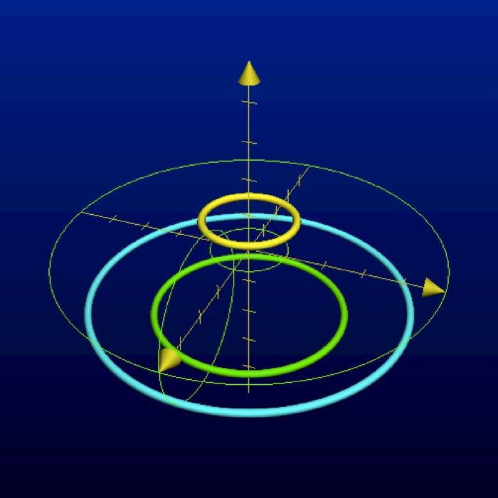
Figure 8. A limit plot of the constant function f⁡(z)=27f(z)=\frac{2}{7} (z∈ℤ2z\in\mathbb{Z}_{2}), in ℝ2\mathbb{R}^{2}
Refer to caption
Figure 9. A limit plot of the same function on the torus 𝕋2\mathbb{T}^{2}           

3.2. Limit plots of linear maps

In this subsection we consider limit plots of linear maps z↦c​zz\mapsto cz (z∈ℤpz\in\mathbb{Z}_{p}) which are finite automaton functions. By Proposition 2.15, the latter takes place if and and only if c∈ℤp∩ℚc\in\mathbb{Z}_{p}\cap\mathbb{Q}.

Proposition 3.5.

Given c∈ℤp∩ℚc\in\mathbb{Z}_{p}\cap\mathbb{Q}, represent c=a/bc=a/b, where a∈ℤa\in\mathbb{Z}, b∈ℕb\in\mathbb{N}, a,ba,b are coprime, p∤bp\nmid b. If 𝔄\mathfrak{A} is an automaton such that f𝔄​(z)=c​zf_{\mathfrak{A}}(z)=cz (z∈ℤp)(z\in\mathbb{Z}_{p}) then 𝐋𝐏⁡(𝔄)={(x𝗆𝗈𝖽1;(c​x)𝗆𝗈𝖽1):x∈ℝ}=𝐂⁡(c,0)\mathbf{LP}(\mathfrak{A})=\{(x\mathbin{\mathsf{mod}}1;(cx)\mathbin{\mathsf{mod}}1)\colon x\in\mathbb{R}\}=\mathbf{C}(c,0) is a cable (with a slope cc) of the unit 2-dimensional real torus 𝕋2\mathbb{T}^{2}. For every c∈ℤp∩ℚc\in\mathbb{Z}_{p}\cap\mathbb{Q} the automaton 𝔄\mathfrak{A} may be taken a finite.

Proof of Proposition 3.5.

By Proposition 2.15,the map z↦c​zz\mapsto cz on ℤp\mathbb{Z}_{p} is an automaton function of a finite automaton if and only if c∈ℤp∩ℚc\in\mathbb{Z}_{p}\cap\mathbb{Q}.

Given x∈[0,1)x\in[0,1), take z∈ℤpz\in\mathbb{Z}_{p} such that limi→∞z𝗆𝗈𝖽pki/pki=x\lim_{i\to\infty}z\mathbin{\mathsf{mod}}p^{k_{i}}/p^{k_{i}}=x for a suitable strictly increasing sequence k1,k2,…∈ℕk_{1},k_{2},\ldots\in\mathbb{N}. As c∈ℤp∩ℚc\in\mathbb{Z}_{p}\cap\mathbb{Q}, then c=u+v/(pt−1)c=u+v/(p^{t}-1) for suitable u∈ℤu\in\mathbb{Z}, t∈ℕt\in\mathbb{N}, v∈{0,1,2,…,pt−2}v\in\{0,1,2,\ldots,p^{t}-2\}, by Proposition 2.2. If t>1t>1, then considering residues of kik_{i} modulo tt we see that at least one residue (say, ℓ∈{0,1,…,t−1}\ell\in\{0,1,\ldots,t-1\}) occurs in the sequence k1,k2,…k_{1},k_{2},\ldots infinitely many times. Therefore limj→∞z𝗆𝗈𝖽prj​t+ℓ/prj​t+ℓ=x\lim_{j\to\infty}z\mathbin{\mathsf{mod}}p^{r_{j}t+\ell}/p^{r_{j}t+\ell}=x for a respective strictly increasing sequence r1,r2,…∈ℕr_{1},r_{2},\ldots\in\mathbb{N}. The latter equality trivially holds when t=1t=1: one just takes rj=kjr_{j}=k_{j} and ℓ=0\ell=0. So further we assume that ki=ri​t+ℓk_{i}=r_{i}t+\ell, i=1,2,…i=1,2,\ldots.

For i=1,2,…i=1,2,\ldots we have that

(c​z)𝗆𝗈𝖽pkipki=1pki​((c𝗆𝗈𝖽pki)​(z𝗆𝗈𝖽pki))𝗆𝗈𝖽pki=(c𝗆𝗈𝖽pki⋅z𝗆𝗈𝖽pkipki)𝗆𝗈𝖽1\frac{(cz)\mathbin{\mathsf{mod}}p^{k_{i}}}{p^{k_{i}}}=\frac{1}{p^{k_{i}}}((c\mathbin{\mathsf{mod}}p^{k_{i}})(z\mathbin{\mathsf{mod}}p^{k_{i}}))\mathbin{\mathsf{mod}}{p^{k_{i}}}=\\ \left(c\mathbin{\mathsf{mod}}p^{k_{i}}\cdot\frac{z\mathbin{\mathsf{mod}}p^{k_{i}}}{p^{k_{i}}}\right)\mathbin{\mathsf{mod}}1 (3.36)

As 0≤ℓ<t0\leq\ell<t and ki=ri​t+ℓk_{i}=r_{i}t+\ell, we have that

c𝗆𝗈𝖽pki=(u+vpt−1)𝗆𝗈𝖽pki=(u−v⋅p(ri+1)​t−1pt−1)𝗆𝗈𝖽pkic\mathbin{\mathsf{mod}}p^{k_{i}}=\left(u+\frac{v}{p^{t}-1}\right)\mathbin{\mathsf{mod}}p^{k_{i}}=\left(u-v\cdot\frac{p^{(r_{i}+1)t}-1}{p^{t}-1}\right)\mathbin{\mathsf{mod}}p^{k_{i}} (3.37)

Note that the argument of 𝗆𝗈𝖽\mathbin{\mathsf{mod}} in the right-hand side of (3.37) is negative once ii is sufficiently large; therefore once ii is large enough then

(u−v⋅p(ri+1)​t−1pt−1)𝗆𝗈𝖽pki=L​pki+u−v⋅p(ri+1)​t−1pt−1\left(u-v\cdot\frac{p^{(r_{i}+1)t}-1}{p^{t}-1}\right)\mathbin{\mathsf{mod}}p^{k_{i}}=Lp^{k_{i}}+u-v\cdot\frac{p^{(r_{i}+1)t}-1}{p^{t}-1}

for a suitable L∈ℕL\in\mathbb{N} which does not depend on ii (actually it is not difficult to see that L=⌈v​pt−ℓ​(pt−1)−1⌉L=\lceil vp^{t-\ell}(p^{t}-1)^{-1}\rceil). Thus,

(c𝗆𝗈𝖽pki⋅z𝗆𝗈𝖽pkipki)𝗆𝗈𝖽1=((L​pki+u−v⋅p(ri+1)​t−1pt−1)⋅z𝗆𝗈𝖽pkipki)𝗆𝗈𝖽1=(L⋅z𝗆𝗈𝖽pki+u⋅z𝗆𝗈𝖽pkipki+vpt−1⋅z𝗆𝗈𝖽pkipki−v​pt−ℓpt−1⋅z𝗆𝗈𝖽pki)𝗆𝗈𝖽1=(c⋅z𝗆𝗈𝖽pkipki−v​pt−ℓpt−1⋅z𝗆𝗈𝖽pki)𝗆𝗈𝖽1\left(c\mathbin{\mathsf{mod}}p^{k_{i}}\cdot\frac{z\mathbin{\mathsf{mod}}p^{k_{i}}}{p^{k_{i}}}\right)\mathbin{\mathsf{mod}}1=\\ \left(\left(Lp^{k_{i}}+u-v\cdot\frac{p^{(r_{i}+1)t}-1}{p^{t}-1}\right)\cdot\frac{z\mathbin{\mathsf{mod}}p^{k_{i}}}{p^{k_{i}}}\right)\mathbin{\mathsf{mod}}1=\\ \left(L\cdot z\mathbin{\mathsf{mod}}p^{k_{i}}+u\cdot\frac{z\mathbin{\mathsf{mod}}p^{k_{i}}}{p^{k_{i}}}+\frac{v}{p^{t}-1}\cdot\frac{z\mathbin{\mathsf{mod}}p^{k_{i}}}{p^{k_{i}}}-\frac{vp^{t-\ell}}{p^{t}-1}\cdot z\mathbin{\mathsf{mod}}p^{k_{i}}\right)\mathbin{\mathsf{mod}}1=\\ \left(c\cdot\frac{z\mathbin{\mathsf{mod}}p^{k_{i}}}{p^{k_{i}}}-\frac{vp^{t-\ell}}{p^{t}-1}\cdot z\mathbin{\mathsf{mod}}p^{k_{i}}\right)\mathbin{\mathsf{mod}}1 (3.38)

Firstly we note that given w∈ℕ0w\in\mathbb{N}_{0}, r∈ℕr\in\mathbb{N}

w​pr​tpt−1𝗆𝗈𝖽1=(w⋅pr​t−1pt−1+wpt−1)𝗆𝗈𝖽1=(wpt−1)𝗆𝗈𝖽1\frac{wp^{rt}}{p^{t}-1}\mathbin{\mathsf{mod}}1=\left(w\cdot\frac{p^{rt}-1}{p^{t}-1}+\frac{w}{p^{t}-1}\right)\mathbin{\mathsf{mod}}1=\left(\frac{w}{p^{t}-1}\right)\mathbin{\mathsf{mod}}1 (3.39)

as pt−1p^{t}-1 is a factor of pr​t−1p^{rt}-1.

Secondly, put z¯=pt−ℓ​z\bar{z}=p^{t-\ell}z, then pt−ℓ​(z𝗆𝗈𝖽pri​t+ℓ)=z¯𝗆𝗈𝖽p(ri+1)​tp^{t-\ell}(z\mathbin{\mathsf{mod}}p^{r_{i}t+\ell})=\bar{z}\mathbin{\mathsf{mod}}{p^{(r_{i}+1)t}} and

x=limi→∞z𝗆𝗈𝖽pkipki=limi→∞z¯𝗆𝗈𝖽pri​tpri​t,x=\lim_{i\to\infty}\frac{z\mathbin{\mathsf{mod}}p^{k_{i}}}{p^{k_{i}}}=\lim_{i\to\infty}\frac{\bar{z}\mathbin{\mathsf{mod}}p^{r_{i}t}}{p^{r_{i}t}},

so in (3.38)

v​pt−ℓpt−1⋅z𝗆𝗈𝖽pri​t+ℓ=vpt−1⋅z¯𝗆𝗈𝖽p(ri+1)​t\frac{vp^{t-\ell}}{p^{t}-1}\cdot z\mathbin{\mathsf{mod}}p^{r_{i}t+\ell}=\frac{v}{p^{t}-1}\cdot\bar{z}\mathbin{\mathsf{mod}}p^{(r_{i}+1)t}

and z¯=z​pt−ℓ∈ℤp\bar{z}=zp^{t-\ell}\in\mathbb{Z}_{p} (recall that ki=ri​t+ℓk_{i}=r_{i}t+\ell where ℓ∈{0,1,…,t−1}\ell\in\{0,1,\ldots,t-1\}).

Let z¯=ζ0+ζ1​pt+ζ2​p2​t+⋯\bar{z}=\zeta_{0}+\zeta_{1}p^{t}+\zeta_{2}p^{2t}+\cdots be a base-ptp^{t} representation of z¯\bar{z} (that is, ζj∈{0,1,…,pt−1}\zeta_{j}\in\{0,1,\ldots,p^{t}-1\}); then by combining (3.36) and (3.38) with (3.39) we get

(c​z)𝗆𝗈𝖽pkipki=(c⋅z𝗆𝗈𝖽pkipki−vpt−1⋅𝗐𝗍pt⁡(z¯𝗆𝗈𝖽p(ri+1)​t))𝗆𝗈𝖽1=(c⋅z𝗆𝗈𝖽pkipki−vpt−1⋅(𝗐𝗍pt⁡(z¯𝗆𝗈𝖽p(ri+1)​t))𝗆𝗈𝖽(pt−1))𝗆𝗈𝖽1\frac{(cz)\mathbin{\mathsf{mod}}p^{k_{i}}}{p^{k_{i}}}=\left(c\cdot\frac{z\mathbin{\mathsf{mod}}p^{k_{i}}}{p^{k_{i}}}-\frac{v}{p^{t}-1}\cdot\wt_{p^{t}}(\bar{z}\mathbin{\mathsf{mod}}p^{(r_{i}+1)t})\right)\mathbin{\mathsf{mod}}1=\\ \left(c\cdot\frac{z\mathbin{\mathsf{mod}}p^{k_{i}}}{p^{k_{i}}}-\frac{v}{p^{t}-1}\cdot(\wt_{p^{t}}(\bar{z}\mathbin{\mathsf{mod}}p^{(r_{i}+1)t}))\mathbin{\mathsf{mod}}(p^{t}-1)\right)\mathbin{\mathsf{mod}}1 (3.40)

where 𝗐𝗍pt\wt_{p^{t}} stands for a ptp^{t}-weight of a natural number, that is, the sum of digits of the number in its base-ptp^{t} representation; i.e., 𝗐𝗍pt⁡(z¯𝗆𝗈𝖽p(ri+1)​t)=ζ0+ζ1+⋯+ζi∈ℕ0\wt_{p^{t}}(\bar{z}\mathbin{\mathsf{mod}}{p^{(r_{i}+1)t}})=\zeta_{0}+\zeta_{1}+\cdots+\zeta_{i}\in\mathbb{N}_{0}. Therefore every limit point of the sequence ((c​z)𝗆𝗈𝖽pki/pki)i=1∞((cz)\mathbin{\mathsf{mod}}p^{k_{i}}/p^{k_{i}})_{i=1}^{\infty} is of the form

(c​x+v​wpt−1)𝗆𝗈𝖽1\left(cx+\frac{vw}{p^{t}-1}\right)\mathbin{\mathsf{mod}}1 (3.41)

for a suitable w∈{0,1,…,pt−2}w\in\{0,1,\ldots,p^{t}-2\}.

We claim that, on the other hand, given x∈[0,1)x\in[0,1) and h∈{0,v,2​v𝗆𝗈𝖽(pt−1),…,((pt−2)​v)𝗆𝗈𝖽(pt−1)}h\in\{0,v,2v\mathbin{\mathsf{mod}}{(p^{t}-1)},\ldots,((p^{t}-2)v)\mathbin{\mathsf{mod}}{(p^{t}-1)}\} (that is, hh lying in the ideal ⟨v⟩\langle v\rangle of the residue ring ℤ/(pt−1)​ℤ\mathbb{Z}/(p^{t}-1)\mathbb{Z} generated by vv) there exists z∈ℤpz\in\mathbb{Z}_{p} and a strictly increasing sequence k1,k2,…,∈ℕk_{1},k_{2},\ldots,\in\mathbb{N} such that

x\displaystyle x =limi→∞z𝗆𝗈𝖽pkipki,and\displaystyle=\lim_{i\to\infty}\frac{z\mathbin{\mathsf{mod}}p^{k_{i}}}{p^{k_{i}}},\ \text{and}
(c​z)𝗆𝗈𝖽pkipki\displaystyle\frac{(cz)\mathbin{\mathsf{mod}}p^{k_{i}}}{p^{k_{i}}} =(c⋅z𝗆𝗈𝖽pkipki+hpt−1)𝗆𝗈𝖽1.\displaystyle=\left(c\cdot\frac{z\mathbin{\mathsf{mod}}p^{k_{i}}}{p^{k_{i}}}+\frac{h}{p^{t}-1}\right)\mathbin{\mathsf{mod}}1.

Indeed, take z∈ℤpz\in\mathbb{Z}_{p} and ki=ri​t+ℓk_{i}=r_{i}t+\ell as above; then all limit points of the sequence ((c​z)𝗆𝗈𝖽pki/pki)i=1∞((cz)\mathbin{\mathsf{mod}}p^{k_{i}}/p^{k_{i}})_{i=1}^{\infty} are of the form (3.41) for, say, w=w1,…,ws∈{0,1,…,pt−2}w=w_{1},\ldots,w_{s}\in\{0,1,\ldots,p^{t}-2\}. If h≡v​wj(mod(pt−1))h\equiv vw_{j}\pmod{(p^{t}-1)} for some j=1,2,…,sj=1,2,\ldots,s, then there is nothing to prove; if h≢v​wj(mod(pt−1))h\not\equiv vw_{j}\pmod{(p^{t}-1)} for all j=1,2,…,sj=1,2,\ldots,s then we tweak zz as follows. As the point of the form (3.41) for w=w1w=w_{1} is a limit point of the sequence ((c​z)𝗆𝗈𝖽pki/pki)i=1∞((cz)\mathbin{\mathsf{mod}}p^{k_{i}}/p^{k_{i}})_{i=1}^{\infty} then (−v​w1)𝗆𝗈𝖽(pt−1)(-vw_{1})\mathbin{\mathsf{mod}}{(p^{t}-1)} occurs in the sequence ((−v⁡((𝗐𝗍pt⁡z¯)𝗆𝗈𝖽p(ri+1)​t))𝗆𝗈𝖽(pt−1))i=1∞((-v((\wt_{p^{t}}\bar{z})\mathbin{\mathsf{mod}}p^{(r_{i}+1)t}))\mathbin{\mathsf{mod}}{(p^{t}-1)})_{i=1}^{\infty} infinitely many times (cf. (3.40)); so some w¯∈{0,1​…,pt−2}\bar{w}\in\{0,1\ldots,p^{t}-2\} such that v​w¯≡v​w1(mod(pt−1))v\bar{w}\equiv vw_{1}\pmod{(p^{t}-1)} occurs in the sequence ((𝗐𝗍pt⁡z¯)𝗆𝗈𝖽p(ri+1)​t)𝗆𝗈𝖽(pt−1)((\wt_{p^{t}}\bar{z})\mathbin{\mathsf{mod}}p^{(r_{i}+1)t})\mathbin{\mathsf{mod}}{(p^{t}-1)} infinitely many times:

w¯=((𝗐𝗍pt⁡z¯)𝗆𝗈𝖽p(ri+1)​t)𝗆𝗈𝖽(pt−1)=(ζ0+ζ1+⋯+ζi)𝗆𝗈𝖽(pt−1)\bar{w}=((\wt_{p^{t}}\bar{z})\mathbin{\mathsf{mod}}p^{(r_{i}+1)t})\mathbin{\mathsf{mod}}{(p^{t}-1)}=(\zeta_{0}+\zeta_{1}+\cdots+\zeta_{i})\mathbin{\mathsf{mod}}(p^{t}-1)

for i=i1,i2,…i=i_{1},i_{2},\ldots (1<i1<i2<…1<i_{1}<i_{2}<\ldots).

As h∈⟨v⟩h\in\langle v\rangle, then h≡−v​w~(mod(pt−1))h\equiv-v\tilde{w}\pmod{(p^{t}-1)} for a suitable w~∈{0,1,…,pt−2}\tilde{w}\in\{0,1,\ldots,p^{t}-2\}. Now put z~=ζ0+ζ~1​pt+ζ2​p2​t+ζ3​p3​t+⋯\tilde{z}=\zeta_{0}+\tilde{\zeta}_{1}p^{t}+\zeta_{2}p^{2t}+\zeta_{3}p^{3t}+\cdots, where ζ~1≡ζ1−w¯+w~(mod(pt−1))\tilde{\zeta}_{1}\equiv\zeta_{1}-\bar{w}+\tilde{w}\pmod{(p^{t}-1)}; then OPENw~=(𝗐𝗍pt⁡z~)𝗆𝗈𝖽p(ri+1)​t)𝗆𝗈𝖽(pt−1)\tilde{w}=(\wt_{p^{t}}\tilde{z})\mathbin{\mathsf{mod}}p^{(r_{i}+1)t})\mathbin{\mathsf{mod}}{(p^{t}-1)}. But limi→∞(z𝗆𝗈𝖽pki/pki)=limi→∞(z~𝗆𝗈𝖽pki/pki)=x\lim_{i\to\infty}(z\mathbin{\mathsf{mod}}p^{k_{i}}/p^{k_{i}})=\lim_{i\to\infty}(\tilde{z}\mathbin{\mathsf{mod}}p^{k_{i}}/p^{k_{i}})=x; so finally we conclude by (3.40) that

limj→∞(c​z~)𝗆𝗈𝖽prij​t+ℓprij​t+ℓ=(c​x+hpt−1)𝗆𝗈𝖽1.\lim_{j\to\infty}\frac{(c\tilde{z})\mathbin{\mathsf{mod}}p^{r_{i_{j}}t+\ell}}{p^{r_{i_{j}}t+\ell}}=\left(cx+\frac{h}{p^{t}-1}\right)\mathbin{\mathsf{mod}}1.

Thus we have shown that

𝐋𝐏(𝔄)={(x;(cx+ept−1)𝗆𝗈𝖽1):x∈[0,1),e∈⟨v⟩}.\mathbf{LP}(\mathfrak{A})=\left\{\left(x;\left(cx+\frac{e}{p^{t}-1}\right)\mathbin{\mathsf{mod}}1\right)\colon x\in[0,1),e\in\langle v\rangle\right\}. (3.42)

But the right-hand side in (3.42) is a cable of torus with slope cc since

{(x;(cx+hpt−1)𝗆𝗈𝖽1):x∈[0,1),h∈⟨v⟩}={(y𝗆𝗈𝖽1;(cy)𝗆𝗈𝖽1):y∈ℝ}.\left\{\left(x;\left(cx+\frac{h}{p^{t}-1}\right)\mathbin{\mathsf{mod}}1\right)\colon x\in[0,1),h\in\langle v\rangle\right\}=\left\{\left(y\mathbin{\mathsf{mod}}1;\left(cy\right)\mathbin{\mathsf{mod}}1\right)\colon y\in\mathbb{R}\right\}. (3.43)

Indeed, if y1=y+ny_{1}=y+n for some n∈ℤn\in\mathbb{Z} then y1𝗆𝗈𝖽1=y𝗆𝗈𝖽1y_{1}\mathbin{\mathsf{mod}}1=y\mathbin{\mathsf{mod}}1 and (c​y1)𝗆𝗈𝖽1=(c⁡(y+n))𝗆𝗈𝖽1=(((u+v​(pt−1)−1)​(y+n))𝗆𝗈𝖽1=(c​y+v​n​(pt−1)−1)𝗆𝗈𝖽1=(c​y+((v​n)𝗆𝗈𝖽(pt−1))⋅(pt−1)−1)𝗆𝗈𝖽1CLOSE(cy_{1})\mathbin{\mathsf{mod}}1=(c(y+n))\mathbin{\mathsf{mod}}1=(((u+v(p^{t}-1)^{-1})(y+n))\mathbin{\mathsf{mod}}1=(cy+vn(p^{t}-1)^{-1})\mathbin{\mathsf{mod}}1=(cy+((vn)\mathbin{\mathsf{mod}}(p^{t}-1))\cdot(p^{t}-1)^{-1})\mathbin{\mathsf{mod}}1, and (3.43) follows. This concludes the proof. ∎

Example 3.6.

Take p=2p=2 and c=5/3c=5/3. Figures 7 and 7 illustrate the limit plot of the function f⁡(z)=(5/3)⋅zf(z)=(5/3)\cdot z in 𝕀2\mathbb{I}^{2} and in 𝕋2\mathbb{T}^{2} respectively.

3.3. Limit plots of affine maps

In this subsection we combine the above two cases (constant maps and linear maps) into a single one to describe limit plots of finite automata whose functions are affine, i.e., of the form z↦c⋅z+qz\mapsto c\cdot z+q (z∈ℤpz\in\mathbb{Z}_{p}). It is evident that the limit plot should be a torus link consisting of several disjoint cables with slopes cc since the limit plot of the constant qq is a collection of parallels, cf. Propositions 3.5 and 3.1. We will give a formal proof of this claim and find the number of knots in the link.

Recall that by Proposition 2.15 the map z↦c⋅z+qz\mapsto c\cdot z+q of ℤp\mathbb{Z}_{p} into itself is an automaton function of some finite automaton if and only if c,q∈ℤp∩ℚc,q\in\mathbb{Z}_{p}\cap\mathbb{Q}. The following proposition shows that we do not alter the limit plot of the map once we replace qq by q+nq+n for arbitrary n∈ℤn\in\mathbb{Z}.

Proposition 3.7.

Given f:z↦c​z+qf\colon z\mapsto cz+q (z∈ℤp)(z\in\mathbb{Z}_{p}) where c,q∈ℤp∩ℚc,q\in\mathbb{Z}_{p}\cap\mathbb{Q}, denote q¯=q𝗆𝗈𝖽1\bar{q}=q\mathbin{\mathsf{mod}}1, f¯:z↦c​z+q¯\bar{f}\colon z\mapsto cz+\bar{q}. Then 𝐋𝐏⁡(f)=𝐋𝐏⁡(f¯)\mathbf{LP}(f)=\mathbf{LP}(\bar{f}).

Proof of Proposition 3.7.

Indeed, once n∈ℤn\in\mathbb{Z} then limk→∞n𝗆𝗈𝖽pk/pk∈{0,1}\lim_{k\to\infty}n\mathbin{\mathsf{mod}}p^{k}/p^{k}\in\{0,1\}; the limit is 11 if and only if nn is negative since given a canonical pp-adic representation n=α0+α1​p+⋯n=\alpha_{0}+\alpha_{1}p+\cdots of a negative n∈ℤn\in\mathbb{Z}, all αi=p−1\alpha_{i}=p-1 if ii is large enough, cf. Subsection 2.2. Therefore (OPENlimk→∞(z+n)𝗆𝗈𝖽pk/pk)𝗆𝗈𝖽1=(limk→∞(z𝗆𝗈𝖽pk+n𝗆𝗈𝖽pk)𝗆𝗈𝖽pk/pk)𝗆𝗈𝖽1=limk→∞(z𝗆𝗈𝖽pk/pk+n𝗆𝗈𝖽pk/pk)𝗆𝗈𝖽1=(limk→∞z𝗆𝗈𝖽pk/pk)𝗆𝗈𝖽1\lim_{k\to\infty}(z+n)\mathbin{\mathsf{mod}}p^{k}/p^{k})\mathbin{\mathsf{mod}}1=(\lim_{k\to\infty}(z\mathbin{\mathsf{mod}}p^{k}+n\mathbin{\mathsf{mod}}p^{k})\mathbin{\mathsf{mod}}p^{k}/p^{k})\mathbin{\mathsf{mod}}1=\lim_{k\to\infty}(z\mathbin{\mathsf{mod}}p^{k}/p^{k}+n\mathbin{\mathsf{mod}}p^{k}/p^{k})\mathbin{\mathsf{mod}}1=(\lim_{k\to\infty}z\mathbin{\mathsf{mod}}p^{k}/p^{k})\mathbin{\mathsf{mod}}1 for all z∈ℤz\in\mathbb{Z}. ∎

Note that the map z↦c​z+q¯z\mapsto cz+\bar{q} from the statement of Proposition 3.7 is an automaton function for a suitable finite automaton 𝔅\mathfrak{B} and 𝐋𝐏⁡(𝔄)=𝐋𝐏⁡(𝔅)\mathbf{LP}(\mathfrak{A})=\mathbf{LP}(\mathfrak{B}), where 𝔄\mathfrak{A} is a finite automaton whose automaton function is ff.

Now we describe limit plot of a special affine map with c=1,q≠0c=1,q\neq 0.

Lemma 3.8.

Given a finite automaton 𝔄\mathfrak{A} whose automaton function is f⁡(z)=z+qf(z)=z+q (q∈ℤp∩ℚq\in\mathbb{Z}_{p}\cap\mathbb{Q} then), the limit plot 𝐋𝐏⁡(𝔄)⊂𝕋2\mathbf{LP}(\mathfrak{A})\subset\mathbb{T}^{2} is a link of a finite number of torus knots which are cables 𝐂⁡(1,e)\mathbf{C}(1,e) where ee is running over 𝐂⁡(q)\mathbf{C}(q).

Proof of Lemma 3.8.

We will prove that once 𝔄\mathfrak{A} is a finite automaton such that f𝔄​(z)=f⁡(z)=z+qf_{\mathfrak{A}}(z)=f(z)=z+q then

𝐋𝐏⁡(𝔄)=⋃e∈𝐂⁡(q)𝐂⁡(1,e).\mathbf{LP}(\mathfrak{A})=\bigcup_{e\in\mathbf{C}(q)}\mathbf{C}(1,e). (3.44)

Note that if e=0e=0 and e∈𝐂⁡(q)e\in\mathbf{C}(q) then 𝐂⁡(q)={0}\mathbf{C}(q)=\{0\} by Proposition 3.1 and there is nothing to prove. So further we assume that e∈𝐂⁡(q)e\in\mathbf{C}(q) and e≠0e\neq 0.

By Proposition 3.7 we may assume that q∈ℤp∩ℚ∩[0,−1)q\in\mathbb{Z}_{p}\cap\mathbb{Q}\cap[0,-1) then q=d⋅(pt−1)−1−1q=d\cdot(p^{t}-1)^{-1}-1 for suitable d∈{0,1​…,pt−2}d\in\{0,1\ldots,p^{t}-2\}, cf. Proposition 2.2; that is, d=ζt−1+ζt−2​p+⋯+ζ0​pt−1d=\zeta_{t-1}+\zeta_{t-2}p+\cdots+\zeta_{0}p^{t-1}, where ζ0,…,ζt−1∈{0,1,…,p−1}\zeta_{0},\ldots,\zeta_{t-1}\in\{0,1,\ldots,p-1\} and therefore

q=−(ζt−1+ζt−2​p+⋯+ζ0​pt−1)​(1+pt+p2​t+⋯)−1=((p−1−ζt−1)+(p−1−ζt−2)​p+⋯+(p−1−ζ0)​pt−1)​(1+pt+p2​t+⋯)q=-(\zeta_{t-1}+\zeta_{t-2}p+\cdots+\zeta_{0}p^{t-1})(1+p^{t}+p^{2t}+\cdots)-1=\\ ((p-1-\zeta_{t-1})+(p-1-\zeta_{t-2})p+\cdots+(p-1-\zeta_{0})p^{t-1})(1+p^{t}+p^{2t}+\cdots)

as (pt−1)−1=−(1+pt+p2​t+⋯)(p^{t}-1)^{-1}=-(1+p^{t}+p^{2t}+\cdots) in ℤp\mathbb{Z}_{p} by Note 2.3. Therefore, in ℤp\mathbb{Z}_{p} the rational number qq can be represented as

q=(η0+η1​p+⋯+ηt−1​pt−1)⋅(1+pt+p2​t+⋯),q=(\eta_{0}+\eta_{1}p+\cdots+\eta_{t-1}p^{t-1})\cdot(1+p^{t}+p^{2t}+\cdots), (3.45)

where ηj=p−1−ζt−1−j\eta_{j}=p-1-\zeta_{t-1-j}, j=0,1,…,t−1j=0,1,\ldots,t-1.

Given x∈[0,1)x\in[0,1) take a sequence ni∈ℕ0n_{i}\in\mathbb{N}_{0}, i=1,2,…i=1,2,\ldots, and a strictly increasing sequence ki∈ℕk_{i}\in\mathbb{N}, i=1,2,…i=1,2,\ldots, such that ki≥⌊logp⁡ni⌋+1k_{i}\geq\lfloor\log_{p}n_{i}\rfloor+1, limi→∞ni/pki=x\lim_{i\to\infty}n_{i}/p^{k_{i}}=x, and ki𝗆𝗈𝖽t=s∈{0,1,…,t−1}k_{i}\mathbin{\mathsf{mod}}t=s\in\{0,1,\ldots,t-1\} for all i=1,2,…i=1,2,\ldots. This is always possible since if, e.g., x=ξ1​p−1+ξ2​p−2+⋯x=\xi_{1}p^{-1}+\xi_{2}p^{-2}+\cdots for suitable ξ1,ξ2,…∈{0,1,…,p−1}\xi_{1},\xi_{2},\ldots\in\{0,1,\ldots,p-1\} then one takes ni=ξ1​pj−1+ξ2​pj−2+⋯+ξj−1n_{i}=\xi_{1}p^{j-1}+\xi_{2}p^{j-2}+\cdots+\xi_{j-1} where j=i​t+sj=it+s and put ki=i​t+sk_{i}=it+s for i=1,2,…i=1,2,\ldots.

Considering a sequence (ni+q)i=0∞(n_{i}+q)_{i=0}^{\infty} in ℤp\mathbb{Z}_{p}, we see that

(ni+q)𝗆𝗈𝖽pkipki=(nipki+q𝗆𝗈𝖽pkipki)𝗆𝗈𝖽1\frac{(n_{i}+q)\mathbin{\mathsf{mod}}p^{k_{i}}}{p^{k_{i}}}=\left(\frac{n_{i}}{p^{k_{i}}}+\frac{q\mathbin{\mathsf{mod}}p^{k_{i}}}{p^{k_{i}}}\right)\mathbin{\mathsf{mod}}1 (3.46)

But ki=i​t+sk_{i}=it+s, s∈{0,1​…,t−1}s\in\{0,1\ldots,t-1\}; thus

(limi→∞(q𝗆𝗈𝖽pkipki))𝗆𝗈𝖽1=(limi→∞((η0+η1​p+⋯+ηs−1​ps−1)​p−s+CLOSECLOSEOPENOPEN(η0+η1​p+⋯+ηt−1​pt−1)⋅(p−i​t−s+p(−i+1)​t−s+⋯+p−t−s)))𝗆𝗈𝖽1=0.(ηs−1​ηs−2​…​η0​ηt−1​ηt−2​…​ηs)∞𝗆𝗈𝖽1\left(\lim_{i\to\infty}\left(\frac{q\mathbin{\mathsf{mod}}p^{k_{i}}}{p^{k_{i}}}\right)\right)\mathbin{\mathsf{mod}}1=(\lim_{i\to\infty}((\eta_{0}+\eta_{1}p+\cdots+\eta_{s-1}p^{s-1})p^{-s}+\\ (\eta_{0}+\eta_{1}p+\cdots+\eta_{t-1}p^{t-1})\cdot(p^{-it-s}+p^{(-i+1)t-s}+\cdots+p^{-t-s})))\mathbin{\mathsf{mod}}1=\\ 0.(\eta_{s-1}\eta_{s-2}\ldots\eta_{0}\eta_{t-1}\eta_{t-2}\ldots\eta_{s})^{\infty}\mathbin{\mathsf{mod}}1 (3.47)

if s≠0s\neq 0, or

(limi→∞(q𝗆𝗈𝖽pkipki))𝗆𝗈𝖽1=(limi→∞((η0+η1​p+⋯+ηt−1​pt−1)⋅(p−i​t+p(−i+1)​t+⋯+p−t)))𝗆𝗈𝖽1=0.(ηt−1​ηt−2​…​η0)∞𝗆𝗈𝖽1\left(\lim_{i\to\infty}\left(\frac{q\mathbin{\mathsf{mod}}p^{k_{i}}}{p^{k_{i}}}\right)\right)\mathbin{\mathsf{mod}}1=\\ (\lim_{i\to\infty}((\eta_{0}+\eta_{1}p+\cdots+\eta_{t-1}p^{t-1})\cdot(p^{-it}+p^{(-i+1)t}+\cdots+p^{-t})))\mathbin{\mathsf{mod}}1=\\ 0.(\eta_{t-1}\eta_{t-2}\ldots\eta_{0})^{\infty}\mathbin{\mathsf{mod}}1 (3.48)

if s=0s=0. From (3.48) and (3.47) it follows that limi→∞(q𝗆𝗈𝖽pki/pki)𝗆𝗈𝖽1∈𝐂⁡(q)\lim_{i\to\infty}(q\mathbin{\mathsf{mod}}p^{k_{i}}/p^{k_{i}})\mathbin{\mathsf{mod}}1\in\mathbf{C}(q) by (3.33) of Note 3.2. Thus we have proved that given x∈[0,1)x\in[0,1) and e∈𝐂⁡(q)e\in\mathbf{C}(q), necessarily (x,(x+e)𝗆𝗈𝖽1)∈𝐋𝐏⁡(𝔄)(x,(x+e)\mathbin{\mathsf{mod}}1)\in\mathbf{LP}(\mathfrak{A}); so 𝐋𝐏⁡(𝔄)⊃𝐂⁡(1,e)\mathbf{LP}(\mathfrak{A})\supset\mathbf{C}(1,e) for every e∈𝐂⁡(b)e\in\mathbf{C}(b).

On the other hand, given z∈ℤpz\in\mathbb{Z}_{p} and a strictly increasing sequence k1,k2,…∈ℕk_{1},k_{2},\ldots\in\mathbb{N}, by combining (3.48) and (3.47) with (3.33) of Note 3.2 we conclude that all limit points of the sequence q𝗆𝗈𝖽pki/pkiq\mathbin{\mathsf{mod}}p^{k_{i}}/p^{k_{i}}, i=1,2,…i=1,2,\ldots, are in 𝐂⁡(q)\mathbf{C}(q) by an argument similar to the above one. Therefore, limit points of the sequence (z𝗆𝗈𝖽pki/pki+q𝗆𝗈𝖽pki/pki)𝗆𝗈𝖽1(z\mathbin{\mathsf{mod}}p^{k_{i}}/p^{k_{i}}+q\mathbin{\mathsf{mod}}p^{k_{i}}/p^{k_{i}})\mathbin{\mathsf{mod}}1, i=1,2,…i=1,2,\ldots, are all of the form (x+e)𝗆𝗈𝖽1(x+e)\mathbin{\mathsf{mod}}1, where xx is an limit point of the sequence z𝗆𝗈𝖽pki/pkiz\mathbin{\mathsf{mod}}p^{k_{i}}/p^{k_{i}} and e∈𝐂⁡(q)e\in\mathbf{C}(q). This proves that 𝐋𝐏(𝔄)⊂∪e∈𝐂⁡(q)𝐂(1,e)\mathbf{LP}(\mathfrak{A})\subset\cup_{e\in\mathbf{C}(q)}\mathbf{C}(1,e) and that (3.44) is true.

∎

Now we are ready to prove the main claim of the Section.

Theorem 3.9.

Given c,q∈ℤpc,q\in\mathbb{Z}_{p}, a map z↦c​z+qz\mapsto cz+q of ℤp\mathbb{Z}_{p} into itself is an automaton function of a finite automaton if and only if c,q∈ℤp∩ℚc,q\in\mathbb{Z}_{p}\cap\mathbb{Q}. Given a finite automaton 𝔄\mathfrak{A} whose automaton function is f⁡(z)=c​z+qf(z)=cz+q for c,q∈ℤp∩ℚc,q\in\mathbb{Z}_{p}\cap\mathbb{Q}, represent c,qc,q as irreducible fractions c=a/bc=a/b, q=a′/b′q=a^{\prime}/b^{\prime}, where a,a′∈ℤa,a^{\prime}\in\mathbb{Z}, b,b′∈ℕb,b^{\prime}\in\mathbb{N} and gcd⁡(a,b)=gcd⁡(a′,b′)=gcd⁡(b,p)=gcd⁡(b′,p)=1\gcd(a,b)=\gcd(a^{\prime},b^{\prime})=\gcd(b,p)=\gcd(b^{\prime},p)=1; then the limit plot 𝐋𝐏⁡(𝔄)⊂𝕋2\mathbf{LP}(\mathfrak{A})\subset\mathbb{T}^{2} is a link of multm⁡p\operatorname{mult}_{m}p torus knots, where m=b′/gcd⁡(b,b′)m=b^{\prime}/\gcd(b,b^{\prime}), and every knot of the link is a cable 𝐂⁡(c,e)\mathbf{C}(c,e) for e∈𝐂⁡(q)e\in\mathbf{C}(q):

𝐋𝐏(𝔄)={(y𝗆𝗈𝖽1;(cy+e)𝗆𝗈𝖽1):y∈ℝ,e∈𝐂(q)}.\mathbf{LP}(\mathfrak{A})=\left\{\left(y\mathbin{\mathsf{mod}}1;\left(cy+e\right)\mathbin{\mathsf{mod}}1\right)\colon y\in\mathbb{R},e\in\mathbf{C}(q)\right\}. (3.49)

Moreover, 𝐂⁡(c,e1)=𝐂⁡(c,e2)\mathbf{C}(c,e_{1})=\mathbf{C}(c,e_{2}) for e1,e2∈𝐂⁡(q)e_{1},e_{2}\in\mathbf{C}(q) if and only if r1≡r2(modm)r_{1}\equiv r_{2}\pmod{m} where ei=(−pri​q)𝗆𝗈𝖽1e_{i}=(-p^{r_{i}}q)\mathbin{\mathsf{mod}}1, i=1,2i=1,2, cf. (3.33).

Note 3.10.

Once m=1m=1, i.e., once b′|bb^{\prime}\mid b, the congruence r1≡r2(modm)r_{1}\equiv r_{2}\pmod{m} holds trivially, mult1⁡p=1\operatorname{mult}_{1}p=1 and the link consists of a single knot; so in that case 𝐂⁡(c,e1)=𝐂⁡(c,e2)\mathbf{C}(c,e_{1})=\mathbf{C}(c,e_{2}) for all e1,e2∈𝐂⁡(q)e_{1},e_{2}\in\mathbf{C}(q).

Proof of Theorem 3.9.

The first statement of the theorem is already proved, see Proposition 2.15.

Given q,c∈ℤp∩ℚq,c\in\mathbb{Z}_{p}\cap\mathbb{Q}, we have that

c\displaystyle c =u+vpt−1,\displaystyle=u+\frac{v}{p^{t}-1}, (3.50)
q\displaystyle q =wpT−1\displaystyle=\frac{w}{p^{T}-1} (3.51)

for suitable u∈ℤu\in\mathbb{Z}, t,T∈ℕt,T\in\mathbb{N}, v∈{0,1,2,…,pt−2}v\in\{0,1,2,\ldots,p^{t}-2\}, w∈{0,1​…,pT−2}w\in\{0,1\ldots,p^{T}-2\}, by Proposition 2.2. Note that we may assume that 0<q<10<q<1 since the set of all limit points of the sequence ((z+q)𝗆𝗈𝖽pk/pk)k=1∞((z+q)\mathbin{\mathsf{mod}}p^{k}/p^{k})_{k=1}^{\infty} is the same as that of the sequence ((z+q𝗆𝗈𝖽1)𝗆𝗈𝖽pk/pk)k=1∞((z+q\mathbin{\mathsf{mod}}1)\mathbin{\mathsf{mod}}p^{k}/p^{k})_{k=1}^{\infty} by Proposition 3.7 and the case q=0q=0 is already considered, cf. Proposition 3.5.

Now we will prove that 𝐋𝐏⁡(𝔄)⊃𝐂⁡(c,e)\mathbf{LP}(\mathfrak{A})\supset\mathbf{C}(c,e) for e∈𝐂⁡(q)e\in\mathbf{C}(q). As q∈ℤp∩ℚ∩(0,1)q\in\mathbb{Z}_{p}\cap\mathbb{Q}\cap(0,1), the canonical pp-adic representation of qq is eventually periodic and the period length of qq is TT, cf. Subsection 2.2. Now fix e∈𝐂⁡(q)e\in\mathbf{C}(q), take corresponding d∈{0,1,…,T−1}d\in\{0,1,\ldots,T-1\} and consider a sequence nj=d+i​T∈ℕn_{j}=d+iT\in\mathbb{N} (j=1,2,…)(j=1,2,\ldots); then limj→∞q𝗆𝗈𝖽pnj/pnj=e\lim_{j\to\infty}q\mathbin{\mathsf{mod}}p^{n_{j}}/p^{n_{j}}=e, cf. the proof of Lemma 3.8. Given x∈[0,1)x\in[0,1) take z∈ℤpz\in\mathbb{Z}_{p} and a sequence 𝒦=(ki=ℓ+ri​t)i=1∞\mathcal{K}=(k_{i}=\ell+r_{i}t)_{i=1}^{\infty} as in the proof of Proposition 3.5; so x=limi→∞z𝗆𝗈𝖽pki/pkix=\lim_{i\to\infty}z\mathbin{\mathsf{mod}}p^{k_{i}}/p^{k_{i}}. Note that if z¯=pm​z\bar{z}=p^{m}z for some m∈ℕ0m\in\mathbb{N}_{0} then x=limi→∞z¯𝗆𝗈𝖽pki+m/pki+mx=\lim_{i\to\infty}\bar{z}\mathbin{\mathsf{mod}}p^{k_{i}+m}/p^{k_{i}+m}; so the proof of Proposition 3.5 remains valid if one substitutes z¯\bar{z} for zz and any strictly increasing subsequence (kˇi)(\check{k}_{i}) of the sequence 𝒦¯=(k¯i=m+ℓ+ri​t)\bar{\mathcal{K}}=(\bar{k}_{i}=m+\ell+r_{i}t) for the sequence 𝒦\mathcal{K}.

We claim that for some m∈ℕ0m\in\mathbb{N}_{0} there exist an increasing sequence js∈ℕj_{s}\in\mathbb{N} and a subsequence (r¯s)s=1∞(\bar{r}_{s})_{s=1}^{\infty} of the sequence (ri)i=1∞(r_{i})_{i=1}^{\infty} such that

m+ℓ+r¯s​t=d+js​T​for all​s=1,2,3,….m+\ell+\bar{r}_{s}t=d+j_{s}T\ \text{for all}\ s=1,2,3,\ldots. (3.52)

Indeed, let D=gcd⁡(T,t)D=\gcd(T,t) be the greatest common divisor of TT and tt; then T=Tˇ​DT=\check{T}D, t=tˇ​Dt=\check{t}D, tˇ\check{t} and Tˇ\check{T} are co-prime. As the infinite sequence (ri)i=1∞(r_{i})_{i=1}^{\infty} is strictly increasing, there exists nˇ∈{0,1,…,tˇ−1}\check{n}\in\{0,1,\ldots,\check{t}-1\} such that ri+nˇ≡0(modTˇ)r_{i}+\check{n}\equiv 0\pmod{\check{T}} for infinitely many i∈ℕi\in\mathbb{N}, say, for i=i1,i2,…i=i_{1},i_{2},\ldots. Put r¯s=ris\bar{r}_{s}=r_{i_{s}}; s=1,2,3,…s=1,2,3,\ldots.

Take the smallest n¯=nˇ+n​Tˇ\bar{n}=\check{n}+n\check{T}, n∈ℕ0n\in\mathbb{N}_{0}, such that d−ℓ+n¯​tˇ​D≥0d-\ell+\bar{n}\check{t}D\geq 0, then put m=d−ℓ+n¯​tˇ​Dm=d-\ell+\bar{n}\check{t}D and find jsj_{s} from the equation (3.52) which now is equivalent to the equation (n¯+r¯s)​tˇ=js​Tˇ(\bar{n}+\bar{r}_{s})\check{t}=j_{s}\check{T}: As n¯+r¯s=hs​Tˇ\bar{n}+\bar{r}_{s}=h_{s}\check{T} for a suitable s∈ℕs\in\mathbb{N} by the definition of n¯\bar{n}, one sees that js=tˇ​hsj_{s}=\check{t}h_{s} for s=1,2,3,…s=1,2,3,\ldots thus proving our claim.

We conclude now that given arbitrary y∈ℝy\in\mathbb{R} and e∈𝐂⁡(q)e\in\mathbf{C}(q) there exist z¯∈ℤp\bar{z}\in\mathbb{Z}_{p} and a sequence 𝒦ˇ=(kˇs=r¯s​t+ℓ+m=d+js​T)\check{\mathcal{K}}=(\check{k}_{s}=\bar{r}_{s}t+\ell+m=d+j_{s}T) such that

y𝗆𝗈𝖽1=x\displaystyle y\mathbin{\mathsf{mod}}1=x =lims→∞z¯𝗆𝗈𝖽pkˇspkˇs,\displaystyle=\lim_{s\to\infty}\frac{\bar{z}\mathbin{\mathsf{mod}}p^{\check{k}_{s}}}{p^{\check{k}_{s}}}, (3.53)
(c​y)𝗆𝗈𝖽1\displaystyle(cy)\mathbin{\mathsf{mod}}1 =lims→∞(c​z¯)𝗆𝗈𝖽pkˇspkˇs,\displaystyle=\lim_{s\to\infty}\frac{(c\bar{z})\mathbin{\mathsf{mod}}p^{\check{k}_{s}}}{p^{\check{k}_{s}}}, (3.54)
e\displaystyle e =lims→∞q𝗆𝗈𝖽pkˇspkˇs;\displaystyle=\lim_{s\to\infty}\frac{q\mathbin{\mathsf{mod}}p^{\check{k}_{s}}}{p^{\check{k}_{s}}}; (3.55)

cf. (3.42), (3.43) and Proposition 3.1. Therefore, lims→∞(c​z¯+q)𝗆𝗈𝖽pkˇs/pkˇs=lims→∞((c​z¯)𝗆𝗈𝖽pkˇs/pkˇs+q𝗆𝗈𝖽pkˇs/pkˇs)𝗆𝗈𝖽1=(c​y+e)𝗆𝗈𝖽1\lim_{s\to\infty}(c\bar{z}+q)\mathbin{\mathsf{mod}}p^{\check{k}_{s}}/p^{\check{k}_{s}}=\lim_{s\to\infty}((c\bar{z})\mathbin{\mathsf{mod}}p^{\check{k}_{s}}/p^{\check{k}_{s}}+q\mathbin{\mathsf{mod}}p^{\check{k}_{s}}/p^{\check{k}_{s}})\mathbin{\mathsf{mod}}1=(cy+e)\mathbin{\mathsf{mod}}1 and so the point (y𝗆𝗈𝖽1,(c​y+e)𝗆𝗈𝖽1)∈𝐂⁡(c,e)(y\mathbin{\mathsf{mod}}1,(cy+e)\mathbin{\mathsf{mod}}1)\in\mathbf{C}(c,e) is in 𝐋𝐏⁡(𝔄)\mathbf{LP}(\mathfrak{A}). Thus we have proved that 𝐋𝐏⁡(𝔄)⊃𝐂⁡(c,e)\mathbf{LP}(\mathfrak{A})\supset\mathbf{C}(c,e) for every e∈𝐂⁡(q)e\in\mathbf{C}(q).

On the other hand, given arbitrary z∈ℤpz\in\mathbb{Z}_{p} and arbitrary strictly increasing sequence k1,k2,…∈ℕk_{1},k_{2},\ldots\in\mathbb{N}, limit points of the point sequence (z𝗆𝗈𝖽pki/pki;(c​z)𝗆𝗈𝖽pki/pki)(z\mathbin{\mathsf{mod}}p^{k_{i}}/p^{k_{i}};(cz)\mathbin{\mathsf{mod}}p^{k_{i}}/p^{k_{i}}) are all in 𝐂⁡(c,0)\mathbf{C}(c,0) by Proposition 3.5 whereas limit points of the sequence q𝗆𝗈𝖽pki/pkiq\mathbin{\mathsf{mod}}p^{k_{i}}/p^{k_{i}} are all in 𝐂⁡(q)\mathbf{C}(q) by Proposition 3.1. Therefore limit points of the point sequence ((,,,))i=1∞=((,,,))i=1∞((z\mathbin{\mathsf{mod}}p^{k_{i}}/p^{k_{i}};(cz+q)\mathbin{\mathsf{mod}}p^{k_{i}}/p^{k_{i}}))_{i=1}^{\infty}=((z\mathbin{\mathsf{mod}}p^{k_{i}}/p^{k_{i}},((cz)\mathbin{\mathsf{mod}}p^{k_{i}}/p^{k_{i}}+q\mathbin{\mathsf{mod}}p^{k_{i}}/p^{k_{i}})\mathbin{\mathsf{mod}}1))_{i=1}^{\infty} are all in ∪e∈𝐂⁡(q)𝐂(c,e)\cup_{e\in\mathbf{C}(q)}\mathbf{C}(c,e). Finally we conclude that 𝐋𝐏(𝔄)=∪e∈𝐂⁡(q)𝐂(c,e)\mathbf{LP}(\mathfrak{A})=\cup_{e\in\mathbf{C}(q)}\mathbf{C}(c,e); or (which is the same) that

𝐋𝐏(𝔄)={(y𝗆𝗈𝖽1;(cy+e)𝗆𝗈𝖽1):y∈ℝ,e∈𝐂(q)}\mathbf{LP}(\mathfrak{A})=\left\{\left(y\mathbin{\mathsf{mod}}1;\left(cy+e\right)\mathbin{\mathsf{mod}}1\right)\colon y\in\mathbb{R},e\in\mathbf{C}(q)\right\} (3.56)

Note that it may happen that 𝐂⁡(c,q)=𝐂⁡(c,q1)\mathbf{C}(c,q)=\mathbf{C}(c,q_{1}) even if q≠q1q\neq q_{1} (and even q∉𝐂⁡(q1)q\notin\mathbf{C}(q_{1})): For instance, (3.42) shows that 𝐂⁡(c,q)=𝐂⁡(c,0)\mathbf{C}(c,q)=\mathbf{C}(c,0) for some q≠0q\neq 0. Therefore to finish the proof we must now calculate the number of pairwise distinct cables 𝐂⁡(c,e)\mathbf{C}(c,e) when e∈𝐂⁡(q)e\in\mathbf{C}(q).

During the proof of Proposition 3.5 we have shown that (in the notation of the proposition under the proof)

{(y𝗆𝗈𝖽1;(c​y)𝗆𝗈𝖽1):y∈ℝ}={(y𝗆𝗈𝖽1;(c​y+jb)𝗆𝗈𝖽1):y∈ℝ}\left\{\left(y\mathbin{\mathsf{mod}}1;\left(cy\right)\mathbin{\mathsf{mod}}1\right)\colon y\in\mathbb{R}\right\}=\left\{\left(y\mathbin{\mathsf{mod}}1;\left(cy+\frac{j}{b}\right)\mathbin{\mathsf{mod}}1\right)\colon y\in\mathbb{R}\right\}

for every j∈ℤj\in\mathbb{Z}, cf. equation (3.43) and the text which follows it. Therefore 𝐂⁡(c,e1)=𝐂⁡(c,e2)\mathbf{C}(c,e_{1})=\mathbf{C}(c,e_{2}) if e1−e2≡(j/b)𝗆𝗈𝖽1e_{1}-e_{2}\equiv(j/b)\mathbin{\mathsf{mod}}1 for some j∈ℤj\in\mathbb{Z}. The converse statement is also true: if 𝐂⁡(c,e1)=𝐂⁡(c,e2)\mathbf{C}(c,e_{1})=\mathbf{C}(c,e_{2}) then e1−e2≡(j/b)𝗆𝗈𝖽1e_{1}-e_{2}\equiv(j/b)\mathbin{\mathsf{mod}}1 for some j∈ℤj\in\mathbb{Z}.

To prove this, for h∈𝐂⁡(q)h\in\mathbf{C}(q) let A⁡(c,h)A(c,h) be a set of all points where the cable 𝐂⁡(c,h)\mathbf{C}(c,h) crosses zero meridian of the torus 𝕋2\mathbb{T}^{2}; that is,

A(c,h)=𝐀𝐏({(0;((c​z)𝗆𝗈𝖽psrpsr+h)𝗆𝗈𝖽1):z∈ℤp,limr→∞z𝗆𝗈𝖽psrpsr=0}),A(c,h)=\mathbf{AP}\left(\left\{\left(0;\left(\frac{(cz)\mathbin{\mathsf{mod}}p^{s_{r}}}{p^{s_{r}}}+h\right)\mathbin{\mathsf{mod}}1\right)\colon z\in\mathbb{Z}_{p},\lim_{r\to\infty}\frac{z\mathbin{\mathsf{mod}}p^{s_{r}}}{p^{s_{r}}}=0\right\}\right),

where s1,s2,…∈ℕs_{1},s_{2},\ldots\in\mathbb{N}, s1<s2<…s_{1}<s_{2}<\ldots; therefore by (3.41)

𝐀𝐏⁡((((c​z)𝗆𝗈𝖽psrpsr+h)𝗆𝗈𝖽1)r=0∞)={(jb+h)𝗆𝗈𝖽1:j=0,1,2,…}.\mathbf{AP}\left(\left(\left(\frac{(cz)\mathbin{\mathsf{mod}}p^{s_{r}}}{p^{s_{r}}}+h\right)\mathbin{\mathsf{mod}}1\right)_{r=0}^{\infty}\right)=\\ \left\{\left(\frac{j}{b}+h\right)\mathbin{\mathsf{mod}}1\colon j=0,1,2,\ldots\right\}. (3.57)

Finally, as 𝐂⁡(c,e1)=𝐂⁡(c,e2)\mathbf{C}(c,e_{1})=\mathbf{C}(c,e_{2}) if and only if A⁡(c,e1)=A⁡(c,e2)A(c,e_{1})=A(c,e_{2}) since the both cables cross zero meridian at a same angle (which is equal to arctan⁡c\arctan c), this means that 𝐂⁡(c,e1)=𝐂⁡(c,e2)\mathbf{C}(c,e_{1})=\mathbf{C}(c,e_{2}) if and only if e1−e2≡j​b−1(mod1)e_{1}-e_{2}\equiv jb^{-1}\pmod{1} for some j∈ℕ0j\in\mathbb{N}_{0}, as claimed.

Now we are able to calculate the number of torus knots (cables) which constitutes the link 𝐋𝐏⁡(𝔄)\mathbf{LP}(\mathfrak{A}). Let for some j1,j2∈{0,1,…,b−1}j_{1},j_{2}\in\{0,1,\ldots,b-1\}, (j1≠j2j_{1}\neq j_{2}) and e1,e2∈𝐂⁡(q)e_{1},e_{2}\in\mathbf{C}(q) the following equality holds:

(j1b+e1)𝗆𝗈𝖽1=(j2b+e2)𝗆𝗈𝖽1.\left(\frac{j_{1}}{b}+e_{1}\right)\mathbin{\mathsf{mod}}1=\left(\frac{j_{2}}{b}+e_{2}\right)\mathbin{\mathsf{mod}}1. (3.58)

We see that ei=−pri(a′b′)𝗆𝗈𝖽1e_{i}=-p^{r_{i}}(\frac{a^{\prime}}{b^{\prime}})\mathbin{\mathsf{mod}}1 for suitable ri∈{0,1,…,(multb′⁡p)−1}r_{i}\in\{0,1,\ldots,(\operatorname{mult}_{b^{\prime}}p)-1\} by Note 3.2 (i=1,2i=1,2). Therefore (3.58) is equivalent to the congruence

pr1​a′b′−pr2​a′b′≡jb(mod1)p^{r_{1}}\frac{a^{\prime}}{b^{\prime}}-p^{r_{2}}\frac{a^{\prime}}{b^{\prime}}\equiv\frac{j}{b}\pmod{1}\

for a suitable j∈{0,1,…,b−1}j\in\{0,1,\ldots,b-1\}; but the latter congruence in turn is equivalent to the congruence

pr2​(pr1−r2−1)​a′​n≡j​m(modn​m​d),p^{r_{2}}\left(p^{r_{1}-r_{2}}-1\right)a^{\prime}n\equiv jm\pmod{nmd}, (3.59)

where d=gcd⁡(b′,b)d=\gcd(b^{\prime},b), m=b′/dm=b^{\prime}/d, n=b/dn=b/d (we assume that r1>r2r_{1}>r_{2} since the case r1=r2r_{1}=r_{2} is trivial). From here it follows that pr2​(pr1−r2−1)​a′​n≡0(modm)p^{r_{2}}\left(p^{r_{1}-r_{2}}-1\right)a^{\prime}n\equiv 0\pmod{m} once m≠1m\neq 1; therefore necessarily r1≡r2(modmultm⁡p)r_{1}\equiv r_{2}\pmod{\operatorname{mult}_{m}p} since gcd⁡(b′,b)=gcd⁡(p,b)=gcd⁡(p,b′)=1\gcd(b^{\prime},b)=\gcd(p,b)=\gcd(p,b^{\prime})=1. So (pr1−r2−1)=m​h\left(p^{r_{1}-r_{2}}-1\right)=mh for a suitable h∈ℕh\in\mathbb{N} and thus (3.59) is equivalent to the congruence pr2​h​a′​n≡j(modn​d)p^{r_{2}}ha^{\prime}n\equiv j\pmod{nd}, and the latter congruence gives the value of jj (modulo b=n​db=nd) so that (3.58) is satisfied. This means that when m≠1m\neq 1, 3.58 holds if and only if r1≡r2(modmultm⁡p)r_{1}\equiv r_{2}\pmod{\operatorname{mult}_{m}p} Thus, if m≠1m\neq 1 (that is, if b′b^{\prime} is not a factor of bb) then the number of pairwise distinct torus knots in the link is multm⁡p\operatorname{mult}_{m}p.

In the remaining case when m=1m=1 (i.e., when b′b^{\prime} divides bb) (3.59) always holds: If pr1−r2≡1(modd)p^{r_{1}-r_{2}}\equiv 1\pmod{d} then we can take j=0j=0 to satisfy (3.59); otherwise the left-hand side of (3.59) just gives an expression for a unique residue jj modulo b=n​db=nd (which thus satisfies (3.59)). Therefore the link consist of a unique cable; so the number of pairwise distinct cables in the link is 1=mult1⁡p1=\operatorname{mult}_{1}p in this case as well. This concludes the proof. ∎

Note 3.11.

In conditions of Theorem 3.9 note that b′|bb^{\prime}|b is the only case when the link 𝐋𝐏⁡(𝔄)\mathbf{LP}(\mathfrak{A}) consists of a single cable . Note also that from the proof of Theorem 3.9 it is clear that if the number #​𝐂​(q)\#\mathbf{C}(q) of points in 𝐂⁡(q)\mathbf{C}(q) is 1 then the link necessarily consists of a single cable. By note 3.2, #​𝐂​(q)=1\#\mathbf{C}(q)=1 if and only if the period length of qq is 1 and therefore q𝗆𝗈𝖽1=0.(ξ)∞𝗆𝗈𝖽1q\mathbin{\mathsf{mod}}1=0.(\xi)^{\infty}\mathbin{\mathsf{mod}}1 for some ξ∈{0,1,…,p−1}\xi\in\{0,1,\ldots,p-1\}).

Example 3.12.

Let p=2p=2 and f⁡(z)=(3/5)⋅z+(1/3)f(z)=(3/5)\cdot z+(1/3). Then in conditions of Theorem 3.9 we have that m=3m=3 and therefore the link consists of mult3⁡2=2\operatorname{mult}_{3}2=2 cables with slopes 3/53/5, cf. Figures 11 and 11.

0,0)(15,15)

Figure 10. Limit plot of the function f⁡(z)=35​z+13f(z)=\frac{3}{5}z+\frac{1}{3}, z∈ℤ2z\in\mathbb{Z}_{2}, in ℝ2\mathbb{R}^{2}
Refer to caption
Figure 11. Limit plot of the same function on the torus 𝕋2\mathbb{T}^{2}    
Corollary 3.13.

There is a one-to-one correspondence between maps of the form f:z↦ab​z+a′b′f\colon z\mapsto\frac{a}{b}z+\frac{a^{\prime}}{b^{\prime}} on ℤp\mathbb{Z}_{p} (where ab,a′b′∈ℤp∩ℚ\frac{a}{b},\frac{a^{\prime}}{b^{\prime}}\in\mathbb{Z}_{p}\cap\mathbb{Q}; a,a′∈ℤa,a^{\prime}\in\mathbb{Z}; b,b′∈ℕb,b^{\prime}\in\mathbb{N}) and collections of multm⁡p\operatorname{mult}_{m}p complex-valued exponential functions ψk:ℝ→ℂ\psi_{k}\colon\mathbb{R}\rightarrow\mathbb{C} of real variable y∈ℝy\in\mathbb{R}

{ψk(y)=ei⁡(ab​y−2​π​pk​a′b′):k=0,1,2,…,(multmp)−1}.\left\{\psi_{k}(y)=e^{i(\frac{a}{b}y-2\pi p^{k}\frac{a^{\prime}}{b^{\prime}})}\colon k=0,1,2,\ldots,(\operatorname{mult}_{m}p)-1\right\}.

Here i∈ℂi\in\mathbb{C} is imaginary unit and m=b′/gcd⁡(b,b′)m=b^{\prime}/\gcd(b,b^{\prime}).

Proof of Corollary 3.13.

Indeed, embedding the unit torus 𝕋2\mathbb{T}^{2} into a 3-dimensional Euclidean space ℝ3\mathbb{R}^{3} and using cylindrical coordinates as in Note 2.27, in view of Theorem 3.9 every knot from the link can be expressed in the form (2.29) with ω=2​π​e\omega=2\pi e for e∈𝐂⁡(q)e\in\mathbf{C}(q) since cos⁡ω\cos\omega and sin⁡ω\sin\omega specifies position of the point where the knot crosses zero meridian of the torus (i.e., when θ≡0(mod2​π)\theta\equiv 0\pmod{2\pi} in (2.29)). But q=a′/b′q=a^{\prime}/b^{\prime} and thus 𝐂(q)={(−pℓ⋅(a′/b′))𝗆𝗈𝖽1:ℓ=0,1,…,(multb′p)−1}\mathbf{C}(q)=\left\{(-p^{\ell}\cdot({a^{\prime}}/{b^{\prime}}))\mathbin{\mathsf{mod}}1\colon\ell=0,1,\ldots,(\operatorname{mult}_{b^{\prime}}p)-1\right\} by (3.32). As two such knots (with accordingly ωi=2​π​ei\omega_{i}=2\pi e_{i}, i=1,2i=1,2) coincide if an only if ω1≡ω2(mod2​π⋅(a/b))\omega_{1}\equiv\omega_{2}\pmod{2\pi\cdot(a/b)} by (2.29), i.e., if and only if e1≡e2(moda/b)e_{1}\equiv e_{2}\pmod{a/b}. But the latter congruence is equivalent to (3.58); so finally the assertion follows from Theorem 3.9. ∎

4. Finite computability

In this section we introduce central notion of the paper, the finite computability, and prove some technical results which will be needed further during the proof of main result of the paper, the affinity of finitely computable smooth functions, cf. further Section 5.

Definition 4.1.

A non-empty point set S⊂𝕀2S\subset\mathbb{I}^{2} (S⊂𝕋2S\subset\mathbb{T}^{2}, S⊂𝕀×𝕊S\subset\mathbb{I}\times\mathbb{S}, S⊂𝕊×𝕀S\subset\mathbb{S}\times\mathbb{I}) is called (ultimately) finitely computable (or, (ultimately) computable by a finite automaton) if there exists a finite automaton 𝔄\mathfrak{A} such that SS is a subset of 𝐏⁡(𝔄)\mathbf{P}(\mathfrak{A}) (of 𝐋𝐏⁡(𝔄)\mathbf{LP}(\mathfrak{A})). We say that the automaton 𝔄\mathfrak{A} (ultimately) computes the set SS; and 𝔄\mathfrak{A} is called an (ultimate) computing automaton of the set SS.

In most further cases given a real function g:D→ℝg\colon D\rightarrow\mathbb{R} with the domain D⊂ℝD\subset\mathbb{R} by the graph of the function (on the torus 𝕋2\mathbb{T}^{2}) we mean the point subset 𝐆D​(g)={(x𝗆𝗈𝖽1;g⁡(x)𝗆𝗈𝖽1):x∈D}⊂𝕋2\mathbf{G}_{D}(g)=\{(x\mathbin{\mathsf{mod}}1;g(x)\mathbin{\mathsf{mod}}1)\colon x\in D\}\subset\mathbb{T}^{2}. However, given a function g:D→Tg\colon D\rightarrow T where either D⊂[0,1]D\subset[0,1] or D⊂𝕊D\subset\mathbb{S} and TT is either [0,1][0,1] or 𝕊\mathbb{S}, we call a graph 𝐆D\mathbf{G}_{D} of the function gg the set {(x¯,g⁡(x)¯):x∈D}\{(\bar{x};\overline{g(x)})\colon x\in D\} where either x¯=x\bar{x}=x if D⊂[0,1]D\subset[0,1] or x¯=x𝗆𝗈𝖽1\bar{x}=x\mathbin{\mathsf{mod}}1 if D⊂𝕊D\subset\mathbb{S} and accordingly either g⁡(x)¯=g⁡(x)\overline{g(x)}=g(x) if T=[0,1]T=[0,1] or g⁡(x)¯=(g⁡(x))𝗆𝗈𝖽1\overline{g(x)}=(g(x))\mathbin{\mathsf{mod}}1 if T=𝕊T=\mathbb{S}. In the sequel we always explain what is meant by 𝐆D​(g)\mathbf{G}_{D}(g) if this is not clear from the context. Also, we may omit the subscript DD when it is clear what is the domain.

Definition 4.2.

Given a real function g:D→ℝg\colon D\rightarrow\mathbb{R} with domain D⊂ℝD\subset\mathbb{R} and an automaton 𝔄\mathfrak{A}, the function gg is called (ultimately) computable by 𝔄\mathfrak{A} at the point x∈Dx\in D if (x𝗆𝗈𝖽1;g⁡(x)𝗆𝗈𝖽1)∈𝐏⁡(𝔄)⊂𝕋2(x\mathbin{\mathsf{mod}}1;g(x)\mathbin{\mathsf{mod}}1)\in\mathbf{P}(\mathfrak{A})\subset\mathbb{T}^{2} ((x𝗆𝗈𝖽1;g⁡(x)𝗆𝗈𝖽1)∈𝐋𝐏⁡(𝔄)⊂𝕋2(x\mathbin{\mathsf{mod}}1;g(x)\mathbin{\mathsf{mod}}1)\in\mathbf{LP}(\mathfrak{A})\subset\mathbb{T}^{2}). Also, if either D⊂[0,1]D\subset[0,1] or D⊂𝕊D\subset\mathbb{S} and g:D→Tg\colon D\rightarrow T where either T=[0,1]T=[0,1] or T=𝕊T=\mathbb{S} we will say that 𝔄\mathfrak{A} (ultimately) computes gg at the point x∈Dx\in D if (x¯,g⁡(x)¯)∈𝐋𝐏⁡(𝔄)(\bar{x};\overline{g(x)})\in\mathbf{LP}(\mathfrak{A}) where either x¯=x\bar{x}=x if D⊂[0,1]D\subset[0,1] or x¯=x𝗆𝗈𝖽1\bar{x}=x\mathbin{\mathsf{mod}}1 if D⊂𝕊D\subset\mathbb{S} and accordingly either g⁡(x)¯=g⁡(x)\overline{g(x)}=g(x) if T=[0,1]T=[0,1] or g⁡(x)¯=(g⁡(x))𝗆𝗈𝖽1\overline{g(x)}=(g(x))\mathbin{\mathsf{mod}}1 if T=𝕊T=\mathbb{S} (cf. Note 2.17)

Given a real function g:D→ℝg\colon D\rightarrow\mathbb{R} with domain D⊂ℝD\subset\mathbb{R}, the function gg is called (ultimately) finitely computable (or, (ultimately) computable by a finite automaton) if there exists a finite automaton 𝔄\mathfrak{A} such that 𝐆⁡(g)⊂𝐏⁡(𝔄)⊂𝕋2\mathbf{G}(g)\subset\mathbf{P}(\mathfrak{A})\subset\mathbb{T}^{2} (𝐆⁡(g)⊂𝐋𝐏⁡(𝔄)⊂𝕋2\mathbf{G}(g)\subset\mathbf{LP}(\mathfrak{A})\subset\mathbb{T}^{2}). The automaton 𝔄\mathfrak{A} which (ultimately) computes the function gg is called the (ultimate) computing automaton of the function gg. In a similar manner we define these notions for the cases when g:D→Tg\colon D\rightarrow T and DD, TT are as above.

4.1. The mark-ups

In loose terms, when assigning a real-valued function f𝔄:[0,1]→[0,1]f^{\mathfrak{A}}\colon[0,1]\rightarrow[0,1] to automaton 𝔄\mathfrak{A} via Monna map 𝗆𝗈𝗇:ℤp→ℝ\operatorname{\mathsf{mon}}:\mathbb{Z}_{p}\to\mathbb{R} (cf. subsection 2.5) one feeds the automaton by a base-pp-expansion of argument x∈[0,1]x\in[0,1] and considers the output as a base-pp expansion of f𝔄​(x)f^{\mathfrak{A}}(x): A base-pp expansion specifies a unique right-infinite word in the alphabet 𝔽p\mathbb{F}_{p} and the automaton ‘reads the word from head to tail’, i.e., is feeded by digits of the base-pp expansion from left to right (i.e., digits on more significant positions are feeded prior to digits on less significant positions); and the output word specifies a base-pp expansion of a unique real number from [0,1][0,1].

To examine functions computed by automata in the meaning of Definition 4.2 it would also be convenient to work with base-pp expansions of real numbers; but the problem is that we need feed the automaton by a right-infinite word in the inverse order ‘from tail (which is at infinity) to head’: Digits on less significant positions (the rightmost ones) should be feeded prior to digits on more significant positions (the leftmost ones). So straightforward inversion is impossible since it is unclear which letter should be the first when feeding the automaton this way; thus output word is undefined and so is the real number whose base-pp expansion is the output word. In this subsection we rigorously specify this inversion and develop some techniques needed in further proofs.

Let a function g:D→𝕊g\colon D\rightarrow\mathbb{S} (or g:D→[0,1]g\colon D\rightarrow[0,1]) whose domain DD is either a subset of a real unit circle 𝕊\mathbb{S} or a subset of a unit segment [0,1][0,1] be ultimately computable by a finite automaton 𝔄=𝔄⁡(s0)\mathfrak{A}=\mathfrak{A}(s_{0}); that is, for any x∈Dx\in D there exists x∈ℤpx\in\mathbb{Z}_{p} such that xx is a limit point of the sequence (z𝗆𝗈𝖽pk/pk)k=1∞(z\mathbin{\mathsf{mod}}p^{k}/p^{k})_{k=1}^{\infty} and g⁡(x)g(x) is a limit point of the sequence ((f𝔄​(z))𝗆𝗈𝖽pk/pk)k=1∞((f_{\mathfrak{A}}(z))\mathbin{\mathsf{mod}}p^{k}/p^{k})_{k=1}^{\infty}, where f𝔄:ℤp→ℤpf_{\mathfrak{A}}\colon\mathbb{Z}_{p}\rightarrow\mathbb{Z}_{p} is automaton function of the automaton 𝔄\mathfrak{A}, cf. Definition 4.2 and Definition 2.16. As said, further to examine finitely computable real functions it is however more convenient to work with automata maps as maps of reals into reals rather than to consider automata functions on pp-adic integers and then represent x∈ℝx\in\mathbb{R} and g⁡(x)∈ℝg(x)\in\mathbb{R} as limit points of the sequences (z𝗆𝗈𝖽pk/pk)k=1∞(z\mathbin{\mathsf{mod}}p^{k}/p^{k})_{k=1}^{\infty} and ((f𝔄​(z))𝗆𝗈𝖽pk/pk)k=1∞((f_{\mathfrak{A}}(z))\mathbin{\mathsf{mod}}p^{k}/p^{k})_{k=1}^{\infty}, respectively.

Further in this subsection we are going to show that once x∈Dx\in D and once x=0.χ1​χ2​…x=0.\chi_{1}\chi_{2}\ldots is a base-pp expansion of xx, we can find a state s=s⁡(x)∈𝒮s=s(x)\in\mathcal{S} of the automaton 𝔄\mathfrak{A} and a strictly increasing infinite sequence of indices 1≤k1<k2<…1\leq k_{1}<k_{2}<\ldots such that the sequence (0.𝔞s(χ1χ2…χkj))j=1∞(0.\mathfrak{a}_{s}(\chi_{1}\chi_{2}\ldots\chi_{k_{j}}))_{j=1}^{\infty} tends to (g⁡(x))𝗆𝗈𝖽1(g(x))\mathbin{\mathsf{mod}}1 (recall that 𝔞s​(ζ1​ζ2​…​ζℓ)\mathfrak{a}_{s}(\zeta_{1}\zeta_{2}\ldots\zeta_{\ell}) is an ℓ\ell-letter output word of the automaton 𝔄⁡(s)\mathfrak{A}(s) whose initial state is ss once the automaton has been feeded by the ℓ\ell-letter input word ζ1​ζ2​…​ζℓ\zeta_{1}\zeta_{2}\ldots\zeta_{\ell}, cf. Subsection 2.3). This means, loosely speaking, that once we feed the automaton 𝔄⁡(s)\mathfrak{A}(s) with approximations 0.χ1​χ2​…​χkj0.\chi_{1}\chi_{2}\ldots\chi_{k_{j}} of xx, the automaton outputs the sequence of approximations 0.𝔞s​(χ1​χ2​…​χkj)0.\mathfrak{a}_{s}(\chi_{1}\chi_{2}\ldots\chi_{k_{j}}) of g⁡(x)g(x), and these sequences tend to xx and to g⁡(x)g(x) accordingly while j→∞j\to\infty. Moreover, we will show that if the function gg is continuous then there exists a state s∈𝒮s\in\mathcal{S} such that all x∈Dx\in D for which s⁡(x)=ss(x)=s constitute a dense subset in DD.

Recall that given x∈(0,1)x\in(0,1), there exists a (right-)infinite word w=γ0​γ1​…w=\gamma_{0}\gamma_{1}\ldots over {0,1,…,p−1}\{0,1,\ldots,p-1\} such that

x=0.γ0​γ1​…=0.w=∑i=0∞γi​p−i−1,x=0.\gamma_{0}\gamma_{1}\ldots=0.w=\sum_{i=0}^{\infty}\gamma_{i}p^{-i-1}, (4.60)

the base-pp expansion of xx. If xx is not of the form x=n/pkx=n/p^{k} for some n=α0+α1​p+⋯+αℓ​pℓ∈{0,1,…,pk−1}n=\alpha_{0}+\alpha_{1}p+\cdots+\alpha_{\ell}p^{\ell}\in\{0,1,\ldots,p^{k}-1\}, where ℓ=𝐥𝐞⁡(n)=⌊logp⁡n⌋+1\ell=\mathbf{le}(n)=\lfloor\log_{p}n\rfloor+1 is the length of the base-pp expansion of n∈ℕ0n\in\mathbb{N}_{0} (recall that we put ⌊logp⁡0⌋=0\lfloor\log_{p}0\rfloor=0, cf. Subsection 2.4), α0,α1,…​αℓ∈{0,1,…,p−1}\alpha_{0},\alpha_{1},\ldots\alpha_{\ell}\in\{0,1,\ldots,p-1\}, then the right-infinite word 𝗐𝗋𝖽⁡(x)=γ0​γ1​…\operatorname{\mathsf{wrd}}(x)=\gamma_{0}\gamma_{1}\ldots over {0,1,…,p−1}\{0,1,\ldots,p-1\} is uniquely defined (and the corresponding xx is said to have a unique base-pp expansion); else there are exactly two infinite words,

𝗐𝗋𝖽r⁡(x)\displaystyle\operatorname{\mathsf{wrd}}^{r}(x) =α0​α1​…​αℓ−1​αℓ​00​…=α0​α1​…​αℓ−1​αℓ​(0)∞\displaystyle=\alpha_{0}\alpha_{1}\ldots\alpha_{\ell-1}\alpha_{\ell}00\ldots=\alpha_{0}\alpha_{1}\ldots\alpha_{\ell-1}\alpha_{\ell}(0)^{\infty} (4.61)
𝗐𝗋𝖽l⁡(x)\displaystyle\operatorname{\mathsf{wrd}}^{l}(x) =α0​α1​…​αℓ−1​(αℓ−1)​(p−1)​(p−1)​…=α0​α1​…​αℓ−1​(αℓ−1)​(p−1)∞,\displaystyle=\alpha_{0}\alpha_{1}\ldots\alpha_{\ell-1}(\alpha_{\ell}-1)(p-1)(p-1)\ldots=\alpha_{0}\alpha_{1}\ldots\alpha_{\ell-1}(\alpha_{\ell}-1)(p-1)^{\infty}, (4.62)

where αℓ≠0\alpha_{\ell}\neq 0, such that x=0.𝗐𝗋𝖽r⁡(x)=0.𝗐𝗋𝖽l⁡(x)x=0.\operatorname{\mathsf{wrd}}_{r}(x)=0.\operatorname{\mathsf{wrd}}_{l}(x). In that case xx is said to have a non-unique base-pp expansion; the corresponding base-pp expansions are called right and left respectively. Both 0 and 1 are assumed to have unique base-pp expansions since 0=0.00​…0=0.00\ldots, 1=0.(p−1)​(p−1)​…1=0.(p-1)(p-1)\ldots; so 𝗐𝗋𝖽⁡(0)=00​…\operatorname{\mathsf{wrd}}(0)=00\ldots, 𝗐𝗋𝖽⁡(1)=(p−1)​(p−1)​…\operatorname{\mathsf{wrd}}(1)=(p-1)(p-1)\ldots. This way we define 𝗐𝗋𝖽⁡(x)\operatorname{\mathsf{wrd}}(x) for all x∈[0,1]x\in[0,1]; and to x=n/pkx=n/p^{k} we will usually put into the correspondence both infinite words 𝗐𝗋𝖽l⁡(x)\operatorname{\mathsf{wrd}}^{l}(x) and 𝗐𝗋𝖽r⁡(x)\operatorname{\mathsf{wrd}}^{r}(x) if converse is not stated explicitly. The only difference in considering a unit circle 𝕊\mathbb{S} rather than the unit segment 𝕀=[0,1]\mathbb{I}=[0,1] is that we identify 0 and 1 and thus have two representations for 0, 0.(0)∞0.(0)^{\infty} and 0=1𝗆𝗈𝖽1=0.(p−1)∞0=1\mathbin{\mathsf{mod}}1=0.(p-1)^{\infty}.

Given a finite word w=αm−1αm−2⋯α0w=\alpha_{m-1}\alpha_{m-2}\cdots\alpha_{0}, we denote via w→\overrightarrow{w} the (right-)infinite word w→=αm−1αm−2⋯α0(0)∞\overrightarrow{w}=\alpha_{m-1}\alpha_{m-2}\cdots\alpha_{0}(0)^{\infty} and we put 0.w→=0.αm−1αm−2⋯α0(0)∞…0.\overrightarrow{w}=0.\alpha_{m-1}\alpha_{m-2}\cdots\alpha_{0}(0)^{\infty}\ldots (note that then 0.w→=ρ⁡(w)0.\overrightarrow{w}=\rho(w)). Of course, 0.w→=0.w=∑i=0m−1αi​p−m+i0.\overrightarrow{w}=0.w=\sum_{i=0}^{m-1}\alpha_{i}p^{-m+i}; but we use notation 0.w→0.\overrightarrow{w} if we want to stress that we deal with infinite base-pp expansion. To unify our notation, we also may write w→=ζ1​ζ2​…\overrightarrow{w}=\zeta_{1}\zeta_{2}\ldots for a (right-)infinite word w=ζ1​ζ2​…w=\zeta_{1}\zeta_{2}\ldots; then 0.w→=0.w=0.ζ1​ζ2​…0.\overrightarrow{w}=0.w=0.\zeta_{1}\zeta_{2}\ldots.

Let w→=γ0​γ1​…\overrightarrow{w}=\gamma_{0}\gamma_{1}\ldots be a (right-)infinite word over 𝔽p={0,1,…,p−1}\mathbb{F}_{p}=\{0,1,\ldots,p-1\}. Given an automaton 𝔄\mathfrak{A} with the initial state ss, we further denote via 𝔞s​(w→)\mathfrak{a}_{s}(\overrightarrow{w}) the set of all limit points of the sequence (ρ⁡(𝔞s​(γ0​γ1​…​γk)))k=0∞(\rho(\mathfrak{a}_{s}(\gamma_{0}\gamma_{1}\ldots\gamma_{k})))_{k=0}^{\infty}. We may omit the subscript ss if it is clear from the context what is the initial state of the automaton.

Given x∈[0,1]x\in[0,1] further 𝔞s​(x)\mathfrak{a}_{s}(x) stands for 𝔞s​(w→​(x))\mathfrak{a}_{s}(\overrightarrow{w}(x)) if xx admits a unique base-pp expansion, and 𝔞s​(x)=𝔞s​(w→​(x)l)∪𝔞s​(w→​(x)r)\mathfrak{a}_{s}(x)=\mathfrak{a}_{s}(\overrightarrow{w}(x)_{l})\cup\mathfrak{a}_{s}(\overrightarrow{w}(x)_{r}) if the expansion is non-unique (thus, if xx admits both left and right base-pp expansions). We also consider 𝔞s​(x)\mathfrak{a}_{s}(x) for x∈𝕊x\in\mathbb{S} rather that for x∈[0,1]x\in[0,1]; in that case we take for 00 both base-pp expansions 0.(0)∞0.(0)^{\infty} and 0.(p−1)∞0.(p-1)^{\infty} (since 0=(0.(p−1)∞)𝗆𝗈𝖽10=(0.(p-1)^{\infty})\mathbin{\mathsf{mod}}1) and reduce modulo 1 all limit points of all sequences (ρ⁡(𝔞s​(γ0​γ1​…​γk)))k=0∞(\rho(\mathfrak{a}_{s}(\gamma_{0}\gamma_{1}\ldots\gamma_{k})))_{k=0}^{\infty}. We further use the same symbol 𝔞s​(x)\mathfrak{a}_{s}(x) independently of whether we consider x∈[0,1]x\in[0,1] or x∈𝕊x\in\mathbb{S}; we make special remarks when this may cause a confusion.

We stress that 𝔞s​(w)\mathfrak{a}_{s}(w) is a uniquely defined finite word whenever w∈𝒲w\in\mathcal{W} is a finite word (and therefore ρ​(𝔞s​(w))\rho(\mathfrak{a}_{s}(w)) consists of a single number), but in the case when ww is an infinite word or ww is a real number from [0,1][0,1] (or w∈𝕊w\in\mathbb{S}), the set 𝔞s​(w)\mathfrak{a}_{s}(w) may contain more than one element.

Given x∈ℚ∩[0,1]x\in\mathbb{Q}\cap[0,1], in view of Lemma 2.10 it is clear that if the automaton 𝔄\mathfrak{A} is finite then 𝔞⁡(x)∈Q∩[0,1]\mathfrak{a}(x)\in Q\cap[0,1] since a real number is rational if and only if its base-pp expansion is eventually periodic. The following propositions reveals some more details about 𝔞⁡(x)\mathfrak{a}(x) for a rational xx; and especially for x=0x=0.

Proposition 4.3.

If 𝔄\mathfrak{A} is finite, x∈ℚ∩[0,1]x\in\mathbb{Q}\cap[0,1] then 𝔞⁡(x)⊂ℚ∩[0,1]\mathfrak{a}(x)\subset\mathbb{Q}\cap[0,1] and 𝔞⁡(x)\mathfrak{a}(x) is a finite set. Moreover, if x∈ℤp∩ℚ∩[0,1]x\in\mathbb{Z}_{p}\cap\mathbb{Q}\cap[0,1] then 𝔞⁡(x)⊂ℤp∩ℚ∩[0,1]\mathfrak{a}(x)\subset\mathbb{Z}_{p}\cap\mathbb{Q}\cap[0,1]. In particular, if x=0∈𝕊x=0\in\mathbb{S} then 𝔞⁡(x)=𝐂⁡(q1)∪𝐂⁡(q2)\mathfrak{a}(x)=\mathbf{C}(q_{1})\cup\mathbf{C}(q_{2}) for suitable q1,q2∈ℤp∩ℚ∩[0,1)q_{1},q_{2}\in\mathbb{Z}_{p}\cap\mathbb{Q}\cap[0,1) (cf. Subsection 3.1). Let a 𝔄\mathfrak{A}-computable function g:D→𝕊g\colon D\rightarrow\mathbb{S} be defined on the domain D⊂𝕊D\subset\mathbb{S} and continuous at 0∈D0\in D. If the domain DD is open then there exists q∈ℤp∩ℚ∩[0,1)q\in\mathbb{Z}_{p}\cap\mathbb{Q}\cap[0,1) such taht 𝔞(0.(0)∞)=𝔞(0.(p−1)∞)∈𝐂(q)\mathfrak{a}(0.(0)^{\infty})=\mathfrak{a}(0.(p-1)^{\infty})\in\mathbf{C}(q); and either 𝔞(0.(0)∞)∈𝐂(q)\mathfrak{a}(0.(0)^{\infty})\in\mathbf{C}(q) or 𝔞(0.(p−1)∞)∈𝐂(q)\mathfrak{a}(0.(p-1)^{\infty})\in\mathbf{C}(q) if the domain DD is half-open and xx is a boundary of DD.

Proof of Proposition 4.3.

Follows from Lemma 2.10 and Proposition 3.1 (see the proof of the latter).

Given x∈ℚ∩[0,1]x\in\mathbb{Q}\cap[0,1], a base-pp expansion of xx is eventually periodic, cf. (2.5): x=0.χ0​…​χk−1​(ξ0​…​ξn−1)∞x=0.\chi_{0}\ldots\chi_{k-1}(\xi_{0}\ldots\xi_{n-1})^{\infty}. Given xx, take n,kn,k the smallest possible (note that then the word v=χ0​…​χk−1v=\chi_{0}\ldots\chi_{k-1} may be empty). From the definition of 𝔞⁡(x)\mathfrak{a}(x) it follows that 𝔞⁡(x)\mathfrak{a}(x) consists of all limit points of the sequences 𝒦⁡(r)=(ρ​((v​(u)k​r))k=K∞CLOSE\mathcal{K}(r)=(\rho(\mathfrak{(}v(u)^{k}r))_{k=K}^{\infty}, where KK is large enough and r∈{ξ0,ξ0​ξ1,…,ξ0​ξ1​…​ξn−1}r\in\{\xi_{0},\xi_{0}\xi_{1},\ldots,\xi_{0}\xi_{1}\ldots\xi_{n-1}\} are all suffixes of the word u=ξ0​…​ξn−1u=\xi_{0}\ldots\xi_{n-1}, for every right-infinite word ww which corresponds to a base-pp expansion of x=0.wx=0.w. As the automaton 𝔄=𝔄⁡(s0)\mathfrak{A}=\mathfrak{A}(s_{0}) is finite, the number of states it reaches after being feeded by either of words rr, where is finite; say, these states are s1,…,sN∈𝒮s_{1},\ldots,s_{N}\in\mathcal{S}. By the same reason, being feeded by the words (u)K(u)^{K} where KK is large enough, the automata 𝔄1=𝔄⁡(s1),…,𝔄N=𝔄⁡(sN)\mathfrak{A}_{1}=\mathfrak{A}(s_{1}),\ldots,\mathfrak{A}_{N}=\mathfrak{A}(s_{N}) output respectively words v1​(u1)K1​t1,…,vN​(uN)KN​tNv_{1}(u_{1})^{K_{1}}t_{1},\ldots,v_{N}(u_{N})^{K_{N}}t_{N}, where the words u1,…,uN,t1,…,tNu_{1},\ldots,u_{N},t_{1},\ldots,t_{N} do not depend on KK, each of the words v1,…,vNv_{1},\ldots,v_{N} is either empty or a prefix of the respective word w1,…,wNw_{1},\ldots,w_{N}, and all the output words v1​(u1)K1​t1,…,vN​(uN)KN​tNv_{1}(u_{1})^{K_{1}}t_{1},\ldots,v_{N}(u_{N})^{K_{N}}t_{N} have the same length as the one of the input word (u)K(u)^{K}, cf. Lemma 2.10. That is, the output words of automata 𝔄i\mathfrak{A}_{i} are all of the form (u¯)L​t(\bar{u})^{L}t, where u¯\bar{u} stands for a cyclically shifted word uu, and after outputting the word (u¯)L​t(\bar{u})^{L}t, each automaton 𝔄i\mathfrak{A}_{i}, i=1,2,…,Ni=1,2,\ldots,N, reaches some of finitely many its states, say, si​1′,…,si​M​(i)′s^{\prime}_{i1},\ldots,s^{\prime}_{iM(i)}. After reaching respective state, the automaton is feeded by the word vv and outputs the corresponding output word vi,j′v^{\prime}_{i,j}, j=1,2,…,M⁡(i)j=1,2,\ldots,M(i). Therefore, all limit points of the sequences 𝒦⁡(r)\mathcal{K}(r) are of the form 0.vi,j′​(u¯i)∞0.{v^{\prime}_{i,j}(\bar{u}_{i})^{\infty}} where u¯i\bar{u}_{i} runs through a (sub)set of all cyclic shifts of the word uiu_{i}, i=1,2,…,Ni=1,2,\ldots,N, j=1,2,…,M⁡(i)j=1,2,\ldots,M(i). But there are only finite number of points of that form; therefore, given a base-pp expansion of x=0.w→x=0.\overrightarrow{w}, the set 𝔞(0.w→)\mathfrak{a}(0.\overrightarrow{w}) is a union of a finite number points of the said form. As every x∈ℚx\in\mathbb{Q} has at most two base-pp expansions, this proves the first claim of the proposition.

If x∈ℤp∩ℚ∩[0,1]x\in\mathbb{Z}_{p}\cap\mathbb{Q}\cap[0,1], then base-pp expansion of xx is purely periodic by Proposition 2.5: x=0.(χ0​…​χn−1)∞x=0.(\chi_{0}\ldots\chi_{n-1})^{\infty}. Therefore once the automaton 𝔄\mathfrak{A} is being feeded by finite words of the form wL​tw^{L}t, where w=χ0​…​χn−1w=\chi_{0}\ldots\chi_{n-1}, tt is a suffix of ww or empty and LL is large enough, by Lemma 2.10 the corresponding output word will be of the form (ut)N⁡(t)​vt(u_{t})^{N(t)}v_{t}, and the number of different words utu_{t} is finite since the number of different words tt is finite. Applying the same argument as above we conclude that all limit points of corresponding sequences are of the form 0.(u)∞0.{(u)^{\infty}} where uu runs through a finite number of finite words. But by Corollary 2.6, all these points are in ℤp∩ℚ∩[0,1]\mathbb{Z}_{p}\cap\mathbb{Q}\cap[0,1]. This proves the second claim of the proposition.

To prove the final claim, we must consider both base-pp representations of zero point of the unit circle 𝕊\mathbb{S}: 0=0.(0)∞0=0.(0)^{\infty} and 0=0.(p−1)∞0=0.(p-1)^{\infty}. Sending a left-infinite zero sequence to the automaton AA, the output sequence will be of the form w∞​tw^{\infty}t by suitable finite words w,tw,t by Lemma 2.10; so 𝔞⁡(0∞)\mathfrak{a}(0^{\infty}) consists of all points of the form 0.(u)∞0.(u)^{\infty}, where uu runs through all cyclic shifts of the word w=χn−1​…​χ0w=\chi_{n-1}\ldots\chi_{0}; therefore 𝔞⁡(0∞)=𝐂⁡(q1)\mathfrak{a}(0^{\infty})=\mathbf{C}(q_{1}) for a suitable q1∈ℤp∩ℚ∩[0,1)q_{1}\in\mathbb{Z}_{p}\cap\mathbb{Q}\cap[0,1), cf. Note 3.2. By the same reason, 𝔞⁡((p−1)∞)=𝐂⁡(q2)\mathfrak{a}((p-1)^{\infty})=\mathbf{C}(q_{2}) for a suitable q2∈ℤp∩ℚ∩[0,1)q_{2}\in\mathbb{Z}_{p}\cap\mathbb{Q}\cap[0,1). In the case when the 𝔄\mathfrak{A}-computable function g:D→𝕊g\colon D\rightarrow\mathbb{S} is continuous at 00 and there exists an open neighborhood UU of 00 such that U⊂DU\subset D then necessarily g⁡(0)∈𝔞⁡(0.0∞)g(0)\in\mathfrak{a}(0.0^{\infty}) and g(0)∈𝔞(0.(p−1)∞)g(0)\in\mathfrak{a}(0.(p-1)^{\infty}); so 𝐂⁡(q1)∩𝐂⁡(q2)≠∅\mathbf{C}(q_{1})\cap\mathbf{C}(q_{2})\neq\emptyset and therefore 𝐂⁡(q1)=𝐂⁡(q2)\mathbf{C}(q_{1})=\mathbf{C}(q_{2}) by Corollary 3.3. If no such neighborhood UU exists then the domain is half-open and 00 is a boundary point; thus due to the continuity of gg at 00 we see that either g⁡(0)∈𝔞⁡(0.0∞)g(0)\in\mathfrak{a}(0.0^{\infty}) or g(0)∈𝔞(0.(p−1)∞)g(0)\in\mathfrak{a}(0.(p-1)^{\infty}) and the conclusion follows.

∎

Corollary 4.4.

Let 𝔄\mathfrak{A} be a finite automaton, let (x;y)∈𝐏⁡(𝔄)⊂𝕋2(x;y)\in\mathbf{P}(\mathfrak{A})\subset\mathbb{T}^{2}, and let x∈ℤp∩ℚ∖{0}x\in\mathbb{Z}_{p}\cap\mathbb{Q}\setminus\{0\}; then y∈ℤp∩ℚy\in\mathbb{Z}_{p}\cap\mathbb{Q}. If x=0x=0 then y∈[0,1)∩ℚy\in[0,1)\cap\mathbb{Q}; moreover, there exists y∈ℤp∩ℚy\in\mathbb{Z}_{p}\cap\mathbb{Q} such that (0,y)∈𝐏⁡(𝔄)(0;y)\in\mathbf{P}(\mathfrak{A}).

Proof of Corollary 4.4.

As x∈ℤp∩ℚx\in\mathbb{Z}_{p}\cap\mathbb{Q} and x∈[0,1)x\in[0,1) then by Corollary 2.7 the base-pp expansion is purely periodic; that is, x=0.wx=0.w, where w∈𝒲∞w\in\mathcal{W}^{\infty} is a right-infinite periodic word: w=(v)∞w=(v)^{\infty} for a suitable finite non-empty word v∈𝒲v\in\mathcal{W}. As (x,y)∈𝐏⁡(𝔄)(x,y)\in\mathbf{P}(\mathfrak{A}) then by Note 2.18 there exists a sequence (ui)i=0∞(u_{i})_{i=0}^{\infty} of finite non-empty words such that limi→∞0.ui=x\lim_{i\to\infty}0.u_{i}=x and simultaneously limi→∞0.𝔞⁡(ui)=y\lim_{i\to\infty}0.\mathfrak{a}(u_{i})=y. Let x≠0x\neq 0; then vv is not a 1-letter zero word: v≠0v\neq 0. Therefore since limi→∞0.ui=x\lim_{i\to\infty}0.u_{i}=x, for all sufficiently large ii the words uiu_{i} must be of the form ui=(v)Li​u¯iu_{i}=(v)^{L_{i}}\bar{u}_{i} where LiL_{i} increases unboundedly while i→∞i\to\infty. Therefore we may assume that the sequence LiL_{i} is strictly increasing (we consider a strictly increasing subsequence of the sequence (Li)(L_{i}) if otherwise) and that all uiu_{i} are of the form ui=(v)Li​u¯iu_{i}=(v)^{L_{i}}\bar{u}_{i}. Let s⁡(i)s(i) be a state the automaton 𝔄\mathfrak{A} reaches after being feeded by the word u¯i\bar{u}_{i} (s⁡(i)=s0s(i)=s_{0} if u¯i=ϕ\bar{u}_{i}=\phi is empty). As the automaton 𝔄\mathfrak{A} is finite, then there are only finitely many pairwise distinct s⁡(i)s(i), say these are s′​(1),…,s′​(n)s^{\prime}(1),\ldots,s^{\prime}(n). Now we consider automata 𝔄⁡(s′​(1)),…,𝔄⁡(s′​(n))\mathfrak{A}(s^{\prime}(1)),\ldots,\mathfrak{A}(s^{\prime}(n)) and apply the same argument as in the proof of the second statement of Proposition 4.3 thus proving that y∈ℤp∩ℚy\in\mathbb{Z}_{p}\cap\mathbb{Q}. The same argument can be applied for the case when x=0x=0 but there exists an infinite sequence of words uiu_{i} whose lengths are increasing unboundedly while i→∞i\to\infty. Therefore the only rest case is now x=0x=0 and once the word sequence (ui)i=0∞(u_{i})_{i=0}^{\infty} is such that limi→∞0.ui=x\lim_{i\to\infty}0.u_{i}=x and lengths of uiu_{i} are bounded; Λ⁡(ui)≤K\Lambda(u_{i})\leq K for all i∈ℕ0i\in\mathbb{N}_{0}. But this just means that for all sufficiently large ii all the words uiu_{i} are KK-letter zero words: ui=(0)Ku_{i}=(0)^{K} for a suitable K∈ℕK\in\mathbb{N}. But then y=0.𝔞⁡((0)K)y=0.\mathfrak{a}((0)^{K}); thus y∈[0,1)∩ℚy\in[0,1)\cap\mathbb{Q}. The last claim of the corollary trivially follows from Proposition 4.3 since once y∈𝔞⁡(0)y\in\mathfrak{a}(0) then (0,y)∈𝐏⁡(𝔄)(0;y)\in\mathbf{P}(\mathfrak{A}) by the definition of 𝐏⁡(𝔄)\mathbf{P}(\mathfrak{A}). ∎

The following definition introduces an important technical notion, the mark-up, which will be used in further proofs:

Definition 4.5.

Given a function g:D→[0,1]g\colon D\rightarrow[0,1] defined on the domain D⊂[0,1]D\subset[0,1], an automaton 𝔄\mathfrak{A}, and a point x∈Dx\in D consider a right-infinite word ww such that x=0.wx=0.w, cf. (4.60), (4.61), (4.62). An infinite strictly increasing sequence i0,i1,i2,…i_{0},i_{1},i_{2},\ldots over ℕ0\mathbb{N}_{0} is called an ss-mark-up of the (right-infinite) word w=γ0​γ1​…w=\gamma_{0}\gamma_{1}\ldots w.r.t. gg and 𝔄\mathfrak{A} (or briefly a mark-up when it is clear what gg, 𝔄\mathfrak{A} and ss are meant) if there exists a state s∈𝒮s\in\mathcal{S} of the automaton 𝔄\mathfrak{A} such that limk→∞ρ⁡(𝔞s​(γ0​γ1​…​γik))=g⁡(x)\lim_{k\to\infty}\rho(\mathfrak{a}_{s}(\gamma_{0}\gamma_{1}\ldots\gamma_{i_{k}}))=g(x).

Remark.

Given x∈D⊂𝕊x\in D\subset\mathbb{S}, the mark-ups of xx are defined exactly in the same way. Note only that the point x=0x=0 of 𝕊\mathbb{S} coincides with the point x=1x=1 and 1=0=0.000​…=0.(p−1)​(p−1)​(p−1)​…∈𝕊1=0=0.000\ldots=0.(p-1)(p-1)(p-1)\ldots\in\mathbb{S} as 𝕊=ℝ𝗆𝗈𝖽1\mathbb{S}=\mathbb{R}\mathbin{\mathsf{mod}}1. In a similar way we define the mark-up when g:D→𝕊g\colon D\rightarrow\mathbb{S}.

The following proposition shows, speaking loosely, that if a continuous real function is finitely computable, then all base-pp expansions of all its arguments can be marked-up:

Proposition 4.6.

Given a continuous function g:(a,b)→[0,1]g\colon(a,b)\rightarrow[0,1] (or, which makes no difference, g:(a,b)→𝕊g\colon(a,b)\rightarrow\mathbb{S} where (a,b)⊂𝕊(a,b)\subset\mathbb{S} is an arc of the unit circle 𝕊\mathbb{S}) let 𝐆⁡(g)⊂𝐏⁡(𝔄)\mathbf{G}(g)\subset\mathbf{P}(\mathfrak{A}) for a suitable finite automaton 𝔄\mathfrak{A}. Then for every x∈(a,b)x\in(a,b) and every infinite word ww such that x=0.wx=0.w there exists an ss-mark-up, for a suitable state s=s⁡(w)∈𝒮s=s(w)\in\mathcal{S} of the automaton 𝔄\mathfrak{A}.

Proof of Proposition 4.6.

The idea of the proof is as follows: Once feeding a finite automaton 𝔄\mathfrak{A} by infinite sequence of finite words γ0,γ0​γ1,γ0​γ1​γ2,…\gamma_{0},\gamma_{0}\gamma_{1},\gamma_{0}\gamma_{1}\gamma_{2},\ldots over ℤp\mathbb{Z}_{p}, the automaton reaches some of its states infinitely many times; this state ss specifies a mark-up (i⁡(s))(i(s)) since corresponding sequences of approximations 0.γ0​…​γi⁡(s)0.\gamma_{0}\ldots\gamma_{i(s)} and 𝔞s(0.γ0…γi⁡(s))\mathfrak{a}_{s}(0.\gamma_{0}\ldots\gamma_{i(s)}) tend accordingly to x=0.γ0​γ1​γ2​…x=0.\gamma_{0}\gamma_{1}\gamma_{2}\ldots and to g⁡(x)g(x) due to the continuity of gg at xx. Now we prove the proposition rigorously.

Firstly consider the case when x∈(a,b)x\in(a,b) has a unique base-pp expansion, say, x=0.γ0​γ1​…=0.wx=0.\gamma_{0}\gamma_{1}\ldots=0.w, where w=γ0​γ1​…w=\gamma_{0}\gamma_{1}\ldots. As g⁡(x)g(x) is 𝔄\mathfrak{A}-computable, there exists a sequence w0,w1,w2,…∈𝒲w_{0},w_{1},w_{2},\ldots\in\mathcal{W} of finite non-empty words such that ρ⁡(w0),ρ⁡(w1),ρ⁡(w2),…∈(a,b)\rho(w_{0}),\rho(w_{1}),\rho(w_{2}),\ldots\in(a,b), limi→∞ρ⁡(wi)=x\lim_{i\to\infty}\rho(w_{i})=x and limj→∞ρ⁡(𝔞⁡(wi))=g⁡(x)\lim_{j\to\infty}\rho(\mathfrak{a}(w_{i}))=g(x). Note that the sequence (Λ⁡(wi))i=0∞(\Lambda(w_{i}))_{i=0}^{\infty} is increasing since otherwise x=n/prx=n/p^{r} for suitable n,r∈ℕ0n,r\in\mathbb{N}_{0} as limi→∞ρ⁡(wi)=x\lim_{i\to\infty}\rho(w_{i})=x and thus xx has a non-unique base-pp expansion. We may assume that (Λ⁡(ωi))i=0∞(\Lambda(\omega_{i}))_{i=0}^{\infty} is a strictly increasing sequence since otherwise we just take a suitable subsequence of (wi)i=0∞(w_{i})_{i=0}^{\infty}. Moreover, by the same reason we may assume that Λ⁡(wi)>i\Lambda(w_{i})>i.

Consider a word sequence w¯0=γ0,w¯1=γ0γ1,w¯2=γ0γ1γ2,…\bar{w}_{0}=\gamma_{0},\bar{w}_{1}=\gamma_{0}\gamma_{1},\bar{w}_{2}=\gamma_{0}\gamma_{1}\gamma_{2},\ldots. As x∈(a,b)x\in(a,b), there exists N∈ℕ0N\in\mathbb{N}_{0} such that 0.w¯i∈(a,b)0.\bar{w}_{i}\in(a,b) once i≥Ni\geq N. Without loss of generality we may assume that N=1N=1. As limi→∞0.wi=0.γ0​γ1​…=x\lim_{i\to\infty}0.w_{i}=0.\gamma_{0}\gamma_{1}\ldots=x, for every n∈ℕ0n\in\mathbb{N}_{0} there exists M⁡(n)∈ℕ0M(n)\in\mathbb{N}_{0}, M⁡(n)≥nM(n)\geq n, such that |0.wi−0.w¯j|<p−n|0.w_{i}-0.\bar{w}_{j}|<p^{-n} provided i,j≥M⁡(n)i,j\geq M(n); therefore as Λ⁡(wi)>i≥M⁡(n)≥n\Lambda(w_{i})>i\geq M(n)\geq n, we conclude that wi=γ0​…​γn​viw_{i}=\gamma_{0}\ldots\gamma_{n}v_{i} for i≥M⁡(n)i\geq M(n) and suitable finite word viv_{i}. Given n∈ℕ0n\in\mathbb{N}_{0}, let M⁡(n)M(n) be the smallest with the said property; this way we obtain an increasing sequence M⁡(0)<M⁡(1)<M⁡(2)<…M(0)<M(1)<M(2)<\ldots. Considering the subsequence (wM⁡(j))j=0∞(w_{M(j)})_{j=0}^{\infty} of the word sequence (wi)i=0∞(w_{i})_{i=0}^{\infty}, we see that wM⁡(j)=γ0​…​γj​rjw_{M(j)}=\gamma_{0}\ldots\gamma_{j}r_{j} for j=0,1,2,…j=0,1,2,\ldots and suitable finite non-empty words rjr_{j}, that limj→∞ρ⁡(wM⁡(j))=x\lim_{j\to\infty}\rho(w_{M(j)})=x and that limj→∞ρ⁡(𝔞⁡(wM⁡(j)))=g⁡(x)\lim_{j\to\infty}\rho(\mathfrak{a}(w_{M(j)}))=g(x). Now to the word sequence (rj)j=0∞(r_{j})_{j=0}^{\infty} we put into the correspondence the sequence OPEN(s⁡(rj)))j=0∞(s(r_{j})))_{j=0}^{\infty} of states of the automaton 𝔄\mathfrak{A}, where s⁡(rj)s(r_{j}) is the state the automaton 𝔄\mathfrak{A} reaches after being feeded by the input word rjr_{j}. As the number of different states of 𝔄\mathfrak{A} is finite, in the sequence (s⁡(rj))j=0∞(s(r_{j}))_{j=0}^{\infty} at least one state, say ss, occurs in the sequence (s⁡(rj))j=0∞(s(r_{j}))_{j=0}^{\infty} infinitely many times; say, for j=j0,j1,j2,…j=j_{0},j_{1},j_{2},\ldots (j0<j1<j2<…j_{0}<j_{1}<j_{2}<\ldots). Therefore

limk→∞ρ⁡(γ0​…​γjk)\displaystyle\lim_{k\to\infty}\rho(\gamma_{0}\ldots\gamma_{j_{k}}) =0.γ0​γ1​…=x\displaystyle=0.\gamma_{0}\gamma_{1}\ldots=x (4.63)
limk→∞ρ⁡(𝔞s​(γ0​…​γjk))\displaystyle\lim_{k\to\infty}\rho(\mathfrak{a}_{s}(\gamma_{0}\ldots\gamma_{j_{k}})) =limk→∞ρ⁡(𝔞⁡(wM⁡(ik)))=g⁡(x)\displaystyle=\lim_{k\to\infty}\rho(\mathfrak{a}(w_{M(i_{k})}))=g(x) (4.64)

Recall that 𝔞=𝔞s0\mathfrak{a}=\mathfrak{a}_{s_{0}} where s0s_{0} is the initial state of the automaton 𝔄=𝔄⁡(s0)\mathfrak{A}=\mathfrak{A}(s_{0}). Note that nowhere in the argument above we have used that gg is continuous.

Now consider the case when x=n/prx=n/p^{r} for suitable n,r∈ℕ0n,r\in\mathbb{N}_{0}, n∈{0,1,…,pr−1}n\in\{0,1,\ldots,p^{r}-1\}. In this case, let 0.γ0​γ1​…0.\gamma_{0}\gamma_{1}\ldots be either of base-pp expansions 𝗐𝗋𝖽r⁡(x)\operatorname{\mathsf{wrd}}^{r}(x), 𝗐𝗋𝖽l⁡(x)\operatorname{\mathsf{wrd}}^{l}(x). We will show that similarly to the case when a base-pp expansion is unique, in the case under consideration there also exist s∈𝒮s\in\mathcal{S} and sequences i0<i1<i2<…i_{0}<i_{1}<i_{2}<\ldots, M⁡(i0)<M⁡(i1)<M⁡(i2)<…M(i_{0})<M(i_{1})<M(i_{2})<\ldots over ℕ0\mathbb{N}_{0} such that M⁡(ik)≥ikM(i_{k})\geq i_{k} for all k∈ℕ0k\in\mathbb{N}_{0} and both (4.63) and (4.64) hold.

For this purpose, consider arbitrary sequence w0,w1,w2,…w_{0},w_{1},w_{2},\ldots of right-infinite words over {0,1,…,p−1}\{0,1,\ldots,p-1\} which are not eventually periodic and such that γ0​…​γi\gamma_{0}\ldots\gamma_{i} is a prefix of wiw_{i} for all i=0,1,2,…i=0,1,2,\ldots. Then limi→∞0.wi=x\lim_{i\to\infty}0.w_{i}=x and therefore all 0.wi∈(a,b)0.w_{i}\in(a,b) once i≥Ii\geq I where II is large enough (we may assume that I=0I=0; otherwise we consider a subsequence (wi)i=I∞(w_{i})_{i=I}^{\infty} rather than the whole sequence (wi)i=0∞(w_{i})_{i=0}^{\infty}). Note that then limi→∞g(0.wi)=g(x)\lim_{i\to\infty}g(0.w_{i})=g(x) as gg is continuous on (a,b)(a,b); therefore there exists a sequence (S⁡(i))i=0∞(S(i))_{i=0}^{\infty} over ℕ\mathbb{N} such that for all i=0,1,2,…i=0,1,2,\ldots the following inequality holds:

|g(0.wi)−g(x)|<p−S⁡(i)|g(0.w_{i})-g(x)|<p^{-S(i)} (4.65)

Moreover, we may assume that the sequence (S⁡(i))i=0∞(S(i))_{i=0}^{\infty} is strictly increasing (if not, we consider a corresponding infinite subsequence of the sequence (wi)i=0∞(w_{i})_{i=0}^{\infty} rather than the whole sequence).

Consider now a word wi=γi​0​γi​1​…w_{i}=\gamma_{i0}\gamma_{i1}\ldots from the above word sequence (note that γi​ℓ=γℓ\gamma_{i\ell}=\gamma_{\ell} for ℓ=1,2,…,i\ell=1,2,\ldots,i). As every 0.wi0.w_{i} is a unique base-pp expansion of the corresponding real number from (a,b)(a,b), there exists a state s⁡(i)s(i) of the automaton 𝔄\mathfrak{A} and a strictly increasing sequence 𝒥⁡(s⁡(i))=(ji​k)k=0∞\mathcal{J}(s(i))=(j_{ik})_{k=0}^{\infty} of numbers from ℕ0\mathbb{N}_{0} such that

limk→∞ρ(𝔞s⁡(i)(γi​0γi​1…γi​ji​k))=g(0.wi),\lim_{k\to\infty}\rho(\mathfrak{a}_{s(i)}(\gamma_{i0}\gamma_{i1}\ldots\gamma_{ij_{ik}}))=g(0.w_{i}), (4.66)

cf. the case we just have considered above at the beginning of the proof of the proposition. Therefore, for any k∈ℕ0k\in\mathbb{N}_{0} there exists K⁡(ji​k)∈ℕK(j_{ik})\in\mathbb{N} such that

|ρ(𝔞s⁡(i)(γi​0γi​1…γi​ji​k))−g(0.wi)|<p−K⁡(ji​k),|\rho(\mathfrak{a}_{s(i)}(\gamma_{i0}\gamma_{i1}\ldots\gamma_{ij_{ik}}))-g(0.w_{i})|<p^{-K(j_{ik})}, (4.67)

and there exists a strictly increasing sequence of kk such that the corresponding sequence of K⁡(ji​k)K(j_{ik}) is also strictly increasing in force of (4.66). Without loss of generality we may assume that the sequence (K⁡(ji​k))k=0∞(K(j_{ik}))_{k=0}^{\infty} is strictly increasing (otherwise we consider a corresponding subsequence of the sequence 𝒥⁡(s⁡(i))\mathcal{J}(s(i))).

As a total number of states of 𝔄\mathfrak{A} is finite, in the infinite sequence (s⁡(i))i=0∞(s(i))_{i=0}^{\infty} at least one state, say ss, occurs infinitely many times. We may assume that s⁡(i)=ss(i)=s for all i∈ℕ0i\in\mathbb{N}_{0}; otherwise we just consider respective subsequence of (wi)i=0∞(w_{i})_{i=0}^{\infty} rather than the whole sequence. As the sequence (ji​k)k=0∞(j_{ik})_{k=0}^{\infty} is strictly increasing, all ji​k>ij_{ik}>i once kk is large enough. Given i∈ℕ0i\in\mathbb{N}_{0}, denote via N⁡(i)∈ℕN(i)\in\mathbb{N} the smallest number such that ji​k>ij_{ik}>i once k≥N⁡(i)k\geq N(i). We again may assume that N⁡(i)=0N(i)=0; if otherwise we will just consider the subsequence (ji​k)k=N⁡(i)∞(j_{ik})_{k=N(i)}^{\infty} rather than the whole sequence (ji​k)k=0∞(j_{ik})_{k=0}^{\infty}. Then γi​0​γi​1​…​γi​ji​k=γ0​…​γi​ri​k\gamma_{i0}\gamma_{i1}\ldots\gamma_{ij_{ik}}=\gamma_{0}\ldots\gamma_{i}r_{ik} for all kk where ri​kr_{ik} is a non-empty finite word.

Let s′​(i,k)∈𝒮s^{\prime}(i,k)\in\mathcal{S} be a state the automaton 𝔄⁡(s)\mathfrak{A}(s) reaches after being feeded by the input word ri​kr_{ik} (the latter state ss is defined above). As the total number of states of 𝔄⁡(s)\mathfrak{A}(s) is finite, in the sequence (s′​(i,k))k=0∞(s^{\prime}(i,k))_{k=0}^{\infty} at least one state, say s′​(i)s^{\prime}(i), occurs infinitely many times. Moreover, by the same reason at least one state, say s′s^{\prime}, occurs in the sequence (s′​(i))i=0∞(s^{\prime}(i))_{i=0}^{\infty} infinitely many times. And again, without loss of generality we may assume that s′​(i,k)=s′s^{\prime}(i,k)=s^{\prime} for all i,ki,k; otherwise we consider corresponding subsequences of the sequences (wi)i=0∞(w_{i})_{i=0}^{\infty} and (ji​k)k=0∞(j_{ik})_{k=0}^{\infty}. Note that being feeded by the input word γi​0​γi​1​…​γi​ji​k=γ0​…​γi​ri​k\gamma_{i0}\gamma_{i1}\ldots\gamma_{ij_{ik}}=\gamma_{0}\ldots\gamma_{i}r_{ik}, the automaton 𝔄⁡(s)\mathfrak{A}(s) (rightmost letters are feeded prior to leftmost ones), the automaton outputs a word of length ji​k+1j_{ik}+1 whose (left) suffix of length i+1i+1 is the word which outputs the automaton 𝔄′=𝔄⁡(s′)\mathfrak{A}^{\prime}=\mathfrak{A}(s^{\prime}) if being feeded by the word γ0​…​γi\gamma_{0}\ldots\gamma_{i}. Therefore

|ρ⁡(𝔞′​(γ0​…​γi))−ρ⁡(𝔞s​(γi​0​γi​1​…​γi​ji​k))|<p−i+1|\rho(\mathfrak{a}^{\prime}(\gamma_{0}\ldots\gamma_{i}))-\rho(\mathfrak{a}_{s}(\gamma_{i0}\gamma_{i1}\ldots\gamma_{ij_{ik}}))|<p^{-i+1} (4.68)

Now combining (4.65), (4.67) and (4.68) we conclude that limi→∞ρ⁡(𝔞′​(γ0​…​γi))=g⁡(x)\lim_{i\to\infty}\rho(\mathfrak{a}^{\prime}(\gamma_{0}\ldots\gamma_{i}))=g(x); but limi→∞ρ⁡(γ0​…​γi)=x\lim_{i\to\infty}\rho(\gamma_{0}\ldots\gamma_{i})=x since 0.γ0​γ1​…0.\gamma_{0}\gamma_{1}\ldots is a base-pp expansion of xx. This finally proves the proposition. ∎

Note 4.7.

Actually during the proof of Proposition 4.6 we have shown that the following claim is true: Let the function g:U→𝕊g\colon U\rightarrow\mathbb{S} (or, g:U→𝕀g\colon U\rightarrow\mathbb{I}) be defined on an open neighbourhood U⊂𝕊U\subset\mathbb{S} (or, U⊂𝕀U\subset\mathbb{I}) of a point xx, let gg be continuous at xx, and let 𝐆⁡(g)⊂𝐏⁡(𝔄)\mathbf{G}(g)\subset\mathbf{P}(\mathfrak{A}) for a suitable finite automaton 𝔄\mathfrak{A}; then there exists a mark-up for every base-pp expansion of xx. Moreover, if g:[a,b]→[0,1]g\colon[a,b]\rightarrow[0,1] is a continuous function on the closed segment [a,b][a,b] then there exist an ss-mark-up for right base-pp expansion of aa and for left base-pp expansion of bb.

Corollary 4.8.

In conditions of Proposition 4.6, if the automaton 𝔄\mathfrak{A} is minimal then 𝐆⁡(g)⊂𝐋𝐏⁡(𝔄)\mathbf{G}(g)\subset\mathbf{LP}(\mathfrak{A}).

Proof of Corollary 4.8.

Follows immediately from Corollary 2.21 by the definition of mark-up. ∎

The following proposition reduces examination of continuous functions computable by a finite automaton 𝔄\mathfrak{A} for the case when the function is defined on a segment for which there exists a state ss of the automaton such that the set of all points from the segment that has ss-mark-ups, is dense in the segment; and so values at these points completely specify the function on the segment.

Proposition 4.9.

Let g:[a,b]→[0,1]g\colon[a,b]\rightarrow[0,1], [a,b]⊂[0,1][a,b]\subset[0,1], be a continuous function; let 𝐆⁡(g)⊂𝐏⁡(𝔄)\mathbf{G}(g)\subset\mathbf{P}(\mathfrak{A}) for a suitable automaton 𝔄\mathfrak{A} whose set of states 𝒮\mathcal{S} is finite. Then [a,b][a,b] is a union of a countably many sub-segments [aj′,bj′]⊂[a,b][a_{j}^{\prime},b_{j}^{\prime}]\subset[a,b], aj′<bj′a_{j}^{\prime}<b_{j}^{\prime}, j=1,2,…j=1,2,\ldots having the following property: For every j=1,2,…j=1,2,\ldots there exists a state sq∈𝒮s_{q}\in\mathcal{S}, q=q⁡(j)q=q(j), such that the set Mq​([aj′,bj′])M_{q}([a_{j}^{\prime},b_{j}^{\prime}]) of all points from [aj′,bj′][a_{j}^{\prime},b_{j}^{\prime}] that have sqs_{q}-mark-ups is dense in [aj′,bj′][a_{j}^{\prime},b_{j}^{\prime}].

Proof of Proposition 4.9.

For s∈𝒮s\in\mathcal{S} denote via 𝒲∞​(s)\mathcal{W}^{\infty}(s) the set of all right-infinite words w∈𝒲∞w\in\mathcal{W}^{\infty} such that 0.w∈(a,b)0.w\in(a,b) and an ss-mark-up for ww exists; put 0.𝒲∞(s)={0.w:w∈𝒲∞(s)}0.\mathcal{W}^{\infty}(s)=\{0.w\colon w\in\mathcal{W}^{\infty}(s)\}.

Given s∈𝒮s\in\mathcal{S} such that 𝒲∞​(s)≠∅\mathcal{W}^{\infty}(s)\neq\emptyset, let 𝐖⁡(s)\mathbf{W}(s) be intersection of the closure 𝐖¯​(s)\overline{\mathbf{W}}(s) of 0.𝒲∞​(s)0.\mathcal{W}^{\infty}(s) with (a,b)(a,b); so 𝐖⁡(s)\mathbf{W}(s) is closed in (a,b)(a,b) w.r.t. the induced topology on (a,b)(a,b) and there are only finitely many pairwise distinct 𝐖⁡(s)\mathbf{W}(s); say, these are 𝐖⁡(s1),…,𝐖⁡(sk)\mathbf{W}(s_{1}),\ldots,\mathbf{W}(s_{k}). Proposition 4.6 implies that 𝐖⁡(s1)∪…∪𝐖⁡(sk)=(a,b)\mathbf{W}(s_{1})\cup\ldots\cup\mathbf{W}(s_{k})=(a,b). We argue that for some 𝐖⁡(s1),…,𝐖⁡(sk)\mathbf{W}(s_{1}),\ldots,\mathbf{W}(s_{k}) their interiors 𝐖​(s1)o,…,𝐖​(sk)o\mathbf{W}(s_{1})^{o},\ldots,\mathbf{W}(s_{k})^{o} are not empty. Indeed, 𝐖​(si)o=𝐖¯​(si)o∩(a,b)\mathbf{W}(s_{i})^{o}=\overline{\mathbf{W}}(s_{i})^{o}\cap(a,b) for all i=1,2,…,ki=1,2,\ldots,k; but from Proposition 4.6 it follows that 𝐖¯​(s1)∪…∪𝐖¯​(sk)=[a,b]\overline{\mathbf{W}}(s_{1})\cup\ldots\cup\overline{\mathbf{W}}(s_{k})=[a,b] and therefore 𝐖¯​(s1)o∪…∪𝐖¯​(sk)o\overline{\mathbf{W}}(s_{1})^{o}\cup\ldots\cup\overline{\mathbf{W}}(s_{k})^{o} is dense in [a,b][a,b] as [a,b][a,b] is Baire, cf. e.g. [1, Theorems 6.16–6.17].

As some (without loss of generality we may assume that all) of the interiors 𝐖¯​(s1)o,…,𝐖¯​(sk)o\overline{\mathbf{W}}(s_{1})^{o},\ldots,\overline{\mathbf{W}}(s_{k})^{o} are non-empty, the interiors are countable unions of open intervals: 𝐖¯(si)o=∪ℓ=1∞(ai​ℓ′,bi​ℓ′)\overline{\mathbf{W}}(s_{i})^{o}=\cup_{\ell=1}^{\infty}(a^{\prime}_{i\ell},b^{\prime}_{i\ell}), ai​ℓ′<bi​ℓ′a^{\prime}_{i\ell}<b^{\prime}_{i\ell}, (i=1,2,…,k)(i=1,2,\ldots,k). Therefore 𝐖¯(si)=∪ℓ=1∞[ai​ℓ′,bi​ℓ′]\overline{\mathbf{W}}(s_{i})=\cup_{\ell=1}^{\infty}[a^{\prime}_{i\ell},b^{\prime}_{i\ell}]. This completes the proof as 𝐖¯​(s1)∪…∪𝐖¯​(sk)=[a,b]\overline{\mathbf{W}}(s_{1})\cup\ldots\cup\overline{\mathbf{W}}(s_{k})=[a,b]. ∎

Corollary 4.10.

In conditions of Proposition 4.9, the segment [a,b][a,b] admits a countable covering by closed sub-segments [aj′,bj′]⊂[a,b][a_{j}^{\prime},b_{j}^{\prime}]\subset[a,b] such that the graph 𝐆⁡(gj)\mathbf{G}(g_{j}) of the restriction of the function gg to the sub-segment [aj′,bj′][a_{j}^{\prime},b_{j}^{\prime}] lies in 𝐏⁡(𝔄⁡(s))⊂𝐏⁡(𝔄)\mathbf{P}(\mathfrak{A}(s))\subset\mathbf{P}(\mathfrak{A}) for a suitable sub-automaton 𝔄⁡(s)\mathfrak{A}(s) of the automaton 𝔄\mathfrak{A}, s=s⁡(j)∈𝒮s=s(j)\in\mathcal{S}.

Proof of Corollary 4.10.

Indeed, the closure of the point set {(x;g⁡(x)):x∈Mq​([aj′,bj′])}\{(x;g(x))\colon x\in M_{q}([a_{j}^{\prime},b_{j}^{\prime}])\} in ℝ2\mathbb{R}^{2} is a graph of the restriction gjg_{j} of the function gg to the segment [aj′,bj′][a_{j}^{\prime},b_{j}^{\prime}] as gjg_{j} is continuous on [aj′,bj′][a_{j}^{\prime},b_{j}^{\prime}]. On the other hand the closure must lie in 𝐏⁡(𝔄⁡(s))\mathbf{P}(\mathfrak{A}(s)) for s=sqs=s_{q} as g⁡(x)=limk→∞ρ⁡(𝔞s​(γ0​…​γik))g(x)=\lim_{k\to\infty}\rho(\mathfrak{a}_{s}(\gamma_{0}\ldots\gamma_{i_{k}})) where x=0.γ0​γ1​…x=0.\gamma_{0}\gamma_{1}\ldots and i0,i1,…i_{0},i_{1},\ldots is an ss-mark-up. Note also that 𝐏⁡(𝔄⁡(s))⊂𝐏⁡(𝔄)\mathbf{P}(\mathfrak{A}(s))\subset\mathbf{P}(\mathfrak{A}) as every state of the automaton 𝔄\mathfrak{A} is reachable from its initial state s0s_{0} (since we consider reachable automata only, cf. Subsection 2.3). ∎

Note 4.11.

From the respective proofs it follows that both Proposition 4.9 and Corollary 4.10 remain true for a continuous function g:[a,b]→𝕊g\colon[a,b]\rightarrow\mathbb{S} as well as for the case when [a,b]⊂𝕊[a,b]\subset\mathbb{S}.

The following theorem shows that we may restrict our considerations of finitely computable continuous functions to the case when computing automata are minimal.

Theorem 4.12.

Given a continuous function g:[a,b]→[0,1]g\colon[a,b]\to[0,1], [a,b]⊂[0,1][a,b]\subset[0,1] such that 𝐆⁡(g)⊂𝐏⁡(𝔄)\mathbf{G}(g)\subset\mathbf{P}(\mathfrak{A}) for a finite automaton 𝔄\mathfrak{A}, there exists a countable covering {[aj′,bj′]⊂[a,b]:j=1,2,…;aj′<bj′}\{[a_{j}^{\prime},b_{j}^{\prime}]\subset[a,b]:j=1,2,\ldots;a_{j}^{\prime}<b_{j}^{\prime}\} of the segment [a,b][a,b] such that for every jj the graph 𝐆⁡(gj)\mathbf{G}(g_{j}) of the restriction gjg_{j} of the function gg to the segment [aj′,bj′][a_{j}^{\prime},b_{j}^{\prime}] lies in 𝐋𝐏⁡(𝔄n)\mathbf{LP}(\mathfrak{A}_{n}) for a suitable minimal sub-automaton 𝔄n\mathfrak{A}_{n} of 𝔄\mathfrak{A}, n=n⁡(j)n=n(j).

Proof of Theorem 4.12.

The state sqs_{q} from Proposition 4.9 is either ergodic or transient, see Subsection 2.3. We consider these two cases separately.

Case 1: The state sqs_{q} is ergodic. As the set Mq​([aj′,bj′])M_{q}([a_{j}^{\prime},b_{j}^{\prime}]) from Proposition 4.9 is dense in [aj′,bj′][a_{j}^{\prime},b_{j}^{\prime}] and gjg_{j} is continuous, every point gj​(x)g_{j}(x) for x∈[aj′,bj′]x\in[a_{j}^{\prime},b_{j}^{\prime}] is a limit of a sequence (g⁡(xi))i=0∞(g(x_{i}))_{i=0}^{\infty} where (xi)i=0∞(x_{i})_{i=0}^{\infty} is a sequence of points from Mq​([aj′,bj′])M_{q}([a_{j}^{\prime},b_{j}^{\prime}]) and (xi)i=0∞(x_{i})_{i=0}^{\infty} tends to xx as ii tends to infinity:

x=\displaystyle x= limi→∞xi;\displaystyle\lim_{i\to\infty}x_{i}; (4.69)
gj​(x)=\displaystyle g_{j}(x)= limi→∞gj​(xi).\displaystyle\lim_{i\to\infty}g_{j}(x_{i}). (4.70)

But xi=0.wix_{i}=0.w_{i} where wiw_{i} is a right-infinite word for which there exists an sqs_{q}-mark-up (cf. the construction of the set Mq​([aj′,bj′])M_{q}([a_{j}^{\prime},b_{j}^{\prime}])); therefore from (4.69)–(4.70) it follows now that there exists a sequence (hℓ)ℓ=0∞(h_{\ell})_{\ell=0}^{\infty} of finite words hℓh_{\ell} of strictly increasing lengths such that

x=\displaystyle x= limℓ→∞0.hℓ;\displaystyle\lim_{\ell\to\infty}0.h_{\ell}; (4.71)
gj​(x)=\displaystyle g_{j}(x)= limℓ→∞ρ⁡(𝔞sq​(hℓ)).\displaystyle\lim_{\ell\to\infty}\rho(\mathfrak{a}_{s_{q}}(h_{\ell})). (4.72)

Indeed, the words hℓh_{\ell} are (left) prefixes of words wq=ω0(q)​ω1(q)​…w_{q}=\omega_{0}^{(q)}\omega_{1}^{(q)}\ldots that correspond to sqs_{q}-mark-up; that is, hℓh_{\ell} are of the form ω0(qℓ)​ω1(qℓ)​…​ωrqℓ,kℓ(qℓ)\omega_{0}^{(q_{\ell})}\omega_{1}^{(q_{\ell})}\ldots\omega_{r_{q_{\ell},k_{\ell}}}^{(q_{\ell})} where the sequence (rqℓ,k)k=0∞(r_{q_{\ell},k})_{k=0}^{\infty} is the sqs_{q}-mark-up of the word wqℓw_{q_{\ell}}. Now, as the state sqs_{q} is ergodic (that is, sqs_{q} a state of a certain minimal sub-automaton, say 𝔄q=𝔄⁡(sq)\mathfrak{A}_{q}=\mathfrak{A}(s_{q}), of the automaton 𝔄\mathfrak{A}, cf. Subsection 2.3), then we just mimic the proof of Theorem 2.20 starting with (2.21)–(2.22) and show that (x,gj​(x))∈𝐋𝐏⁡(𝔄q)(x,g_{j}(x))\in\mathbf{LP}(\mathfrak{A}_{q}).

Case 2: Now let the state sqs_{q} from Proposition 4.9 be not ergodic (whence transient). Thus there exists a finite word u=α0​…​αk−1u=\alpha_{0}\ldots\alpha_{k-1} such that after the automaton 𝔄~=𝔄⁡(sq)\tilde{\mathfrak{A}}=\mathfrak{A}(s_{q}) has been feeded by the word uu (rightmost letters are feeded to the automaton prior to leftmost ones), the automaton reaches some ergodic state (say tt) which is a state of a minimal sub-automaton 𝔄′=𝔄⁡(t)\mathfrak{A}^{\prime}=\mathfrak{A}(t), see Subsection 2.3. Note that then all words of the form v​uvu have the same property, for all v∈𝒲ϕv\in\mathcal{W}_{\phi}: After being feeded by v​uvu, the automaton reaches some state from the set of states of 𝔄′\mathfrak{A}^{\prime} due to the minimality of 𝔄′\mathfrak{A}^{\prime}. Therefore, the set Bq⊂ℤpB_{q}\subset\mathbb{Z}_{p} of all pp-adic integers whose base-pp expansions (cf. Subsection 2.2) are left-infinite words w∈𝒲∞w\in\mathcal{W}^{\infty} such that if the automaton 𝔄⁡(sq)\mathfrak{A}(s_{q}) while being feeded by the word ww reaches at a finite step some ergodic state (that is, reaches a state which is a state of some minimal automaton of 𝔄\mathfrak{A}) is a union of balls of non-zero radii in ℤp\mathbb{Z}_{p}; thus, the set BqB_{q} is an open subset in ℤp\mathbb{Z}_{p} since every ball of a non-zero radius is open in ℤp\mathbb{Z}_{p} w.r.t. the pp-adic topology, cf. Subsection 2.2. Hence the set Aq=ℤp∖BqA_{q}=\mathbb{Z}_{p}\setminus B_{q} is a closed subset of ℤp\mathbb{Z}_{p}; and the set AqA_{q} consists of all pp-adic integers such that if the automaton 𝔄⁡(sq)\mathfrak{A}(s_{q}) is being feeded by a left-infinite word that is a base-pp expansion of some pp-adic integer from AqA_{q}, the automaton 𝔄\mathfrak{A} never reaches an ergodic state. Let PqP_{q} be the set of all finite prefixes of words from AqA_{q}; denote 𝐏q\mathbf{P}_{q} a closure of the set 0.Pq={0.w:w∈Pq}0.P_{q}=\{0.w\colon w\in P_{q}\} in ℝ\mathbb{R}.

Claim:The interior of 𝐏q\mathbf{P}_{q} is empty (therefore 𝐏q\mathbf{P}_{q} is nowhere dense in [0,1][0,1]).

Indeed, if not then 𝐏q\mathbf{P}_{q} contains an open interval (aq,bq)(a_{q},b_{q}). Take a finite non-empty word uu such that aq<0.u<bqa_{q}<0.u<b_{q}. As 𝐏q⊃(aq,bq)\mathbf{P}_{q}\supset(a_{q},b_{q}) then, given an arbitrary finite non-empty word v=α1​…​αkv=\alpha_{1}\ldots\alpha_{k} where αk≠0\alpha_{k}\neq 0, there exists a sequence 𝒲⁡(v)=(wi)i=1∞\mathcal{W}(v)=(w_{i})_{i=1}^{\infty} of finite non-empty words wi∈Pqw_{i}\in P_{q} such that limi→∞0.wi=0.u​v∈(aq,bq)\lim_{i\to\infty}0.w_{i}=0.uv\in(a_{q},b_{q}) (recall that u​vuv is a concatenation of words uu and vv). Therefore either u​v∈Pquv\in P_{q} (thus v∈Pqv\in P_{q} by the construction of PqP_{q}) or 𝒲⁡(v)\mathcal{W}(v) contains an infinite subsequence of words of the form wi′=u​α1​…​αk′​(p−1)riw_{i}^{\prime}=u\alpha_{1}\ldots\alpha_{k}^{\prime}(p-1)^{r_{i}} where αk′=αk−1\alpha_{k}^{\prime}=\alpha_{k}-1, r1<r2<…r_{1}<r_{2}<\ldots (recall that (p−1)ri(p-1)^{r_{i}} is a word of length rir_{i} all whose letters are p−1p-1); hence by the construction of PqP_{q} there exists an infinite sequence wi′′=α1​…​αk′​(p−1)riw_{i}^{\prime\prime}=\alpha_{1}\ldots\alpha_{k}^{\prime}(p-1)^{r_{i}} over PqP_{q}. Thus we conclude that once n∈ℕn\in\mathbb{N}, the closure of AqA_{q} in ℤp\mathbb{Z}_{p} (thus, the very set AqA_{q} itself as it is closed) must either contain nn or −n-n (recall that negative rational integers in ℤp\mathbb{Z}_{p} are exactly that ones whose canonical pp-adic expansions have only a finitely many terms with coefficients other than p−1p-1, cf. Subsection 2.2). But this implies that Aq=ℤpA_{q}=\mathbb{Z}_{p} as the set {±n:n∈ℕ}\{\pm n\colon n\in\mathbb{N}\} (where ++ or −- are taken in arbitrary order) is dense in ℤp\mathbb{Z}_{p}. On the other hand, by the construction the set AqA_{q} consists of all pp-adic integers such that if the automaton 𝔄⁡(sq)\mathfrak{A}(s_{q}) is being feeded by a left-infinite word that is a base-pp expansion of some pp-adic integer from AqA_{q}, the automaton 𝔄\mathfrak{A} never reaches an ergodic state; therefore the equality Aq=ℤpA_{q}=\mathbb{Z}_{p} contradicts our assumption that sqs_{q} is transient (since then there must exist a left-infinite word ww such that at a finite step the automaton 𝔄~=𝔄⁡(sq)\tilde{\mathfrak{A}}=\mathfrak{A}(s_{q}) reaches an ergodic state if being feeded by ww). This proves our claim.

Denote now via f~\tilde{f} an automaton function of the automaton 𝔄~=𝔄⁡(sq)\tilde{\mathfrak{A}}=\mathfrak{A}(s_{q}); and for k=1,2,…k=1,2,\ldots put

Ek′​(f~)={(z𝗆𝗈𝖽pkpk;f~​(z)𝗆𝗈𝖽pkpk)∈𝕀2:z∈ℤp∖Aq=Bq}E_{k}^{\prime}(\tilde{f})=\left\{\left({\frac{{z\mathbin{\mathsf{mod}}p^{k}}}{p^{k}};\frac{{\tilde{f}(z)\mathbin{\mathsf{mod}}p^{k}}}{p^{k}}}\right)\in\mathbb{I}^{2}\colon z\in\mathbb{Z}_{p}\setminus A_{q}=B_{q}\right\} (4.73)

a point set in the unit real square 𝕀2=[0,1]×[0,1]\mathbb{I}^{2}=[0,1]\times[0,1]; then take a union E′(f~)=∪k=1∞Ek′(f~)E^{\prime}(\tilde{f})=\cup_{k=1}^{\infty}E_{k}^{\prime}(\tilde{f}); denote via 𝐏′​(𝔄~)=𝐏′​(f~)\mathbf{P}^{\prime}(\tilde{\mathfrak{A}})=\mathbf{P}^{\prime}(\tilde{f}) a closure (in topology of ℝ2\mathbb{R}^{2}) of the set E′​(f~)E^{\prime}(\tilde{f}) (cf. (2.17)). Denote via gjg_{j} a restriction of the function gg to [aj′,bj′][a_{j}^{\prime},b_{j}^{\prime}]. As the function gjg_{j} is continuous on [aj′,bj′][a_{j}^{\prime},b_{j}^{\prime}] (cf. Corollary 4.10) and 𝐆⁡(g)⊂𝐏⁡(𝔄)\mathbf{G}(g)\subset\mathbf{P}(\mathfrak{A}), then necessarily 𝐆⁡(gj)⊂𝐏′​(𝔄~)\mathbf{G}(g_{j})\subset\mathbf{P}^{\prime}(\tilde{\mathfrak{A}}) since the set 𝐏q\mathbf{P}_{q} is nowhere dense in [aj′,bj′][a_{j}^{\prime},b_{j}^{\prime}] by Claim 1.

As the set 𝒮\mathcal{S} of all states of the automaton 𝔄\mathfrak{A} is finite, there are only finitely many ergodic components in 𝒮\mathcal{S}; say they are 𝒮1,…,𝒮m⊂𝒮\mathcal{S}_{1},\ldots,\mathcal{S}_{m}\subset\mathcal{S}. Given an ergodic component 𝒮n\mathcal{S}_{n} (n=1,2,…,m)(n=1,2,\ldots,m) denote

En={(z𝗆𝗈𝖽pkpk;f~​(z)𝗆𝗈𝖽pkpk)∈𝕀2:z∈Bq,k>kn(z)}E_{n}=\left\{\left({\frac{{z\mathbin{\mathsf{mod}}p^{k}}}{p^{k}};\frac{{\tilde{f}(z)\mathbin{\mathsf{mod}}p^{k}}}{p^{k}}}\right)\in\mathbb{I}^{2}\colon z\in B_{q},k>k_{n}(z)\right\}

where kn​(z)k_{n}(z) is the smallest k∈ℕk\in\mathbb{N} such that after the automaton 𝔄~=𝔄⁡(sq)\tilde{\mathfrak{A}}=\mathfrak{A}(s_{q}) has been feeded by the word 𝗐𝗋𝖽⁡(z𝗆𝗈𝖽pkn​(z))\operatorname{\mathsf{wrd}}(z\mathbin{\mathsf{mod}}p^{k_{n}(z)}), the automaton reaches a state from 𝒮n\mathcal{S}_{n}. Then the union E=∪n=1mEnE=\cup_{n=1}^{m}E_{n} is disjoint and 𝐏′​(𝔄~)\mathbf{P}^{\prime}(\tilde{\mathfrak{A}}) is a closure of EE by (4.73). Therefore 𝐏′(𝔄~)=∪n=1m𝐄n\mathbf{P}^{\prime}(\tilde{\mathfrak{A}})=\cup_{n=1}^{m}\mathbf{E}_{n} where 𝐄n\mathbf{E}_{n} is a closure of EnE_{n} in 𝕀2\mathbb{I}^{2}; hence 𝐆(gj)=∪n=1m(𝐆(gj)∩𝐄n)\mathbf{G}(g_{j})=\cup_{n=1}^{m}(\mathbf{G}(g_{j})\cap\mathbf{E}_{n}). Note that from the definition of 𝐏⁡(𝔄)\mathbf{P}(\mathfrak{A}) (cf. Subsection 2.5) it follows that 𝐄n=𝐏⁡(𝔄n)\mathbf{E}_{n}=\mathbf{P}(\mathfrak{A}_{n}) where 𝔄n\mathfrak{A}_{n} is a minimal sub-automaton (of the automaton 𝔄\mathfrak{A}) whose set of states is 𝒮n\mathcal{S}_{n}.

Further, as the function gjg_{j} is continuous on [aj′,bj′][a_{j}^{\prime},b_{j}^{\prime}], the set 𝐆⁡(gj)\mathbf{G}(g_{j}) is closed in 𝕀2\mathbb{I}^{2}; therefore the set 𝐆n=𝐆⁡(gj)∩𝐄n\mathbf{G}_{n}=\mathbf{G}(g_{j})\cap\mathbf{E}_{n} is closed in ℝ2\mathbb{R}^{2}. Hence, the set 𝐑n={x∈[aj′,bj′]:(x,g⁡(x))∈𝐄n}\mathbf{R}_{n}=\{x\in[a_{j}^{\prime},b_{j}^{\prime}]\colon(x,g(x))\in\mathbf{E}_{n}\} is closed in ℝ\mathbb{R} and [aj′,bj′]=∪n=1m𝐑n[a_{j}^{\prime},b_{j}^{\prime}]=\cup_{n=1}^{m}\mathbf{R}_{n}. Now by argument similar to that from the proof of Proposition 4.9 we conclude that some of the interiors 𝐑no\mathbf{R}_{n}^{o} must be non-empty and hence either of the non-empty interiors is a union of a countably many open intervals. By taking closures of the intervals we see that [aj′,bj′][a_{j}^{\prime},b_{j}^{\prime}] is a union of the closures, that is, [aj′,bj′][a_{j}^{\prime},b_{j}^{\prime}] is a union of a countably many its closed sub-segments [aj.i′,bj.i′][a_{j.i}^{\prime},b_{j.i}^{\prime}] (i∈ℕ0)(i\in\mathbb{N}_{0}) of non-zero lengths, and the graph of the restriction gj.ig_{j.i} of gjg_{j} to either of the sub-segments lies in 𝐄n=𝐏⁡(𝔄n)\mathbf{E}_{n}=\mathbf{P}(\mathfrak{A}_{n}) for a suitable n∈{1,2,…,m}n\in\{1,2,\ldots,m\}. Now we apply Proposition 4.9 substituting gj.ig_{j.i} for gg and [aj.i′,bj.i′][a_{j.i}^{\prime},b_{j.i}^{\prime}] for [a,b][a,b]; but as every sqs_{q} from the statement of Proposition 4.9 is now a state of the minimal sub-automaton 𝔄n\mathfrak{A}_{n}, we now are in conditions of Case 1. Therefore 𝐆⁡(gj.i)⊂𝐋𝐏⁡(𝔄n​(sq))\mathbf{G}(g_{j.i})\subset\mathbf{LP}(\mathfrak{A}_{n}(s_{q})); but 𝐋𝐏⁡(𝔄n​(s))=𝐋𝐏⁡(𝔄n​(t))\mathbf{LP}(\mathfrak{A}_{n}(s))=\mathbf{LP}(\mathfrak{A}_{n}(t)) for all states s,ts,t of the automaton 𝐋𝐏​(𝔄n​(sq))\mathbf{LP}(\mathfrak{A}_{n}(s_{q})) due to the minimality of the automaton, cf. Note 2.22.

This finally proves the theorem.

∎

Note 4.13.

From the proof of Theorem 4.12 it follows that the theorem remains true for a continuous function g:[a,b]→𝕊g\colon[a,b]\rightarrow\mathbb{S} as well as for the case when [a,b]⊂𝕊[a,b]\subset\mathbb{S}.

The following proposition shows that we may if necessary consider only finitely computable continuous functions defined everywhere on the unit segment [0,1][0,1] rather than on sub-segments of [0,1][0,1].

Proposition 4.14 (The similarity).

If a continuous function g:[a,b]→𝕊g\colon[a,b]\rightarrow\mathbb{S}, [a,b]⊂[0,1][a,b]\subset[0,1], is such that 𝐆[a,b]​(g)⊂𝐏​(𝔄)\mathbf{G}_{[a,b]}(g)\subset\mathbf{P}(\mathfrak{A}) for a suitable finite automaton 𝔄=𝔄⁡(s0)\mathfrak{A}=\mathfrak{A}(s_{0}) then for every n,m∈ℕ0n,m\in\mathbb{N}_{0} such that m≥⌊logp⁡n⌋+1m\geq\lfloor\log_{p}n\rfloor+1 and n/pm,(n+1)/pm∈[a,b]n/p^{m},(n+1)/p^{m}\in[a,b] the function gd​(x)=(pm​g​(d+p−m​x))𝗆𝗈𝖽1g_{d}(x)=(p^{m}g(d+p^{-m}x))\mathbin{\mathsf{mod}}1, where d=n​p−md=np^{-m}, is continuous on [0,1][0,1], and 𝐆[0,1]​(gd)⊂𝐏⁡(𝔄)\mathbf{G}_{[0,1]}(g_{d})\subset\mathbf{P}(\mathfrak{A}).

Proof of Proposition 4.14.

As a base-pp expansion of dd is d=0.χ0​…​χm−1​00​…d=0.\chi_{0}\ldots\chi_{m-1}00\ldots then, given a base-pp expansion for x=0.ζ0​ζ1​…∈[0,1]x=0.\zeta_{0}\zeta_{1}\ldots\in[0,1], a base-pp expansion for d+x​p−md+xp^{-m} is d+x​p−m=0.χ0​…​χm−1​ζ0​ζ1​…d+xp^{-m}=0.\chi_{0}\ldots\chi_{m-1}\zeta_{0}\zeta_{1}\ldots and d+x​p−m∈[a,b]d+xp^{-m}\in[a,b] for all right-infinite words ζ0​ζ1​…\zeta_{0}\zeta_{1}\ldots (thus, for all x∈[0,1]x\in[0,1]). Therefore if i0<i1<i2<…i_{0}<i_{1}<i_{2}<\ldots is a mark-up for χ0​…​χm−1​ζ0​ζ1​…\chi_{0}\ldots\chi_{m-1}\zeta_{0}\zeta_{1}\ldots (cf. Proposition 4.6) then (jm=ir+m−m)m=0∞(j_{m}=i_{r+m}-m)_{m=0}^{\infty}, where r=min⁡{ℓ:iℓ>m}r=\min\{\ell\colon i_{\ell}>m\}, is an ss-mark-up of the infinite word ζ0​ζ1​…\zeta_{0}\zeta_{1}\ldots for a suitable state s∈𝒮s\in\mathcal{S} of the automaton 𝔄=𝔄⁡(s0)\mathfrak{A}=\mathfrak{A}(s_{0}) w.r.t. the function gg. Hence,

limk→∞ρ⁡(𝔞s​(ζ0​ζ1​…​ζjk))≡(pm⋅(g⁡(d+xpm)))(mod1)\lim_{k\to\infty}\rho(\mathfrak{a}_{s}(\zeta_{0}\zeta_{1}\ldots\zeta_{j_{k}}))\equiv\left(p^{m}\cdot\left(g\left(d+\frac{x}{p^{m}}\right)\right)\right)\pmod{1} (4.74)

as ρ⁡(𝔞s​(ζ0​ζ1​…​ζjk))=(pm​(ρ⁡(𝔞s​(χ0​…​χm−1​ζ0​ζ1​…​ζjk))))𝗆𝗈𝖽1\rho(\mathfrak{a}_{s}(\zeta_{0}\zeta_{1}\ldots\zeta_{j_{k}}))=(p^{m}(\rho(\mathfrak{a}_{s}(\chi_{0}\ldots\chi_{m-1}\zeta_{0}\zeta_{1}\ldots\zeta_{j_{k}}))))\mathbin{\mathsf{mod}}1. By our assumption on reachability of the automaton 𝔄\mathfrak{A} (cf. Subsection 2.3), there exists a finite word u=u⁡(s)u=u(s) such that the automaton 𝔄\mathfrak{A} being feeded by uu reaches the state ss and outputs the corresponding finite word u′=𝔞s0​(u)u^{\prime}=\mathfrak{a}_{s_{0}}(u); therefore the automaton 𝔄=𝔄⁡(s0)\mathfrak{A}=\mathfrak{A}(s_{0}) being feeded by a concatenated finite word ζ0​ζ1​…​ζjk​u\zeta_{0}\zeta_{1}\ldots\zeta_{j_{k}}u outputs the concatenated finite word 𝔞s​(ζ0​ζ1​…​ζjk)​u′\mathfrak{a}_{s}(\zeta_{0}\zeta_{1}\ldots\zeta_{j_{k}})u^{\prime}. But limk→∞ρ⁡(𝔞s0​(ζ0​ζ1​…​ζjk​u))=limk→∞ρ⁡(𝔞s​(ζ0​ζ1​…​ζjk)​u′)=limk→∞ρ⁡(𝔞s​(ζ0​ζ1​…​ζjk))\lim_{k\to\infty}\rho(\mathfrak{a}_{s_{0}}(\zeta_{0}\zeta_{1}\ldots\zeta_{j_{k}}u))=\lim_{k\to\infty}\rho(\mathfrak{a}_{s}(\zeta_{0}\zeta_{1}\ldots\zeta_{j_{k}})u^{\prime})=\lim_{k\to\infty}\rho(\mathfrak{a}_{s}(\zeta_{0}\zeta_{1}\ldots\zeta_{j_{k}})) and simultaneously x=limk→∞ρ⁡(ζ0​ζ1​…​ζjk​u)=limk→∞ρ⁡(ζ0​ζ1​…​ζjk)x=\lim_{k\to\infty}\rho(\zeta_{0}\zeta_{1}\ldots\zeta_{j_{k}}u)=\lim_{k\to\infty}\rho(\zeta_{0}\zeta_{1}\ldots\zeta_{j_{k}}) since the words u,u′u,u^{\prime} are finite and fixed; therefore (x;gd​(x)𝗆𝗈𝖽1)∈𝐏⁡(𝔄)(x;g_{d}(x)\mathbin{\mathsf{mod}}1)\in\mathbf{P}(\mathfrak{A}) for all x∈[0,1]x\in[0,1] in view of (4.74).

The function gdg_{d} is conjugated to a continuous function by a continuous map and therefore is also continuous: Once e,h∈[0,1]e,h\in[0,1] are such that |e−h|<p−K⁡(L)|e-h|<p^{-K(L)} to ensure that |g⁡(d+p−m​e)−g⁡(d+p−m)​h|<p−L|g(d+p^{-m}e)-g(d+p^{-m})h|<p^{-L} for a sufficiently large L∈ℕL\in\mathbb{N} then |gd​(e)−gd​(h)|<p−L+m|g_{d}(e)-g_{d}(h)|<p^{-L+m}.

∎

Corollary 4.15.

If a continuous function g:[a,b]→𝕊g\colon[a,b]\rightarrow\mathbb{S}, [a,b]⊂[0,1][a,b]\subset[0,1], is such that 𝐆(a,b)​(g)⊂𝐏​(𝔄)\mathbf{G}_{(a,b)}(g)\subset\mathbf{P}(\mathfrak{A}) for a suitable finite automaton 𝔄=𝔄⁡(s0)\mathfrak{A}=\mathfrak{A}(s_{0}) then for every n,m∈ℕ0n,m\in\mathbb{N}_{0} such that m≥⌊logp⁡n⌋+1m\geq\lfloor\log_{p}n\rfloor+1 and d=n/pm∈[a,b)d=n/p^{m}\in[a,b)

  • •

    the function gd,M​(x)=(pM​g​(d+p−M​x))𝗆𝗈𝖽1g_{d,M}(x)=(p^{M}g(d+p^{-M}x))\mathbin{\mathsf{mod}}1 is continuous on [0,1][0,1] for all sufficiently large M≥mM\geq m, and

  • •

    𝐆[0,1]​(gd,M)⊂𝐏⁡(𝔄)\mathbf{G}_{[0,1]}(g_{d,M})\subset\mathbf{P}(\mathfrak{A}).

Proof of Corollary 4.15.

Indeed, in the proof of Proposition 4.14 as a base-pp expansion for d=n​p−md=np^{-m} just use 0.χ0​…​χm−1​(0)M−m0.\chi_{0}\ldots\chi_{m-1}(0)^{M-m} where M≥mM\geq m is large enough so that 0.χ0​…​χm−1​(0)M−m−1​1∈[a,b]0.\chi_{0}\ldots\chi_{m-1}(0)^{M-m-1}1\in[a,b]. Note that nowhere in the proof of the proposition we used that some of χ0,…,χm−1\chi_{0},\ldots,\chi_{m-1} are not zero. ∎

Note 4.16.

Corollary 4.15 shows that given any point d′∈[a,b)d^{\prime}\in[a,b) and a rational approximation d=n​p−md=np^{-m} of d′d^{\prime}, the graph of the function gg on a sufficiently small closed neighbourhood [a′,b′][a^{\prime},b^{\prime}] of the point d′≠b′d^{\prime}\neq b^{\prime} is similar to the graph of the function gd,Mg_{d,M} on [0,1][0,1] where d=n​p−md=np^{-m} and MM is large enough.

Summarizing results of the current subsection we may say that while considering a continuous function g:[a,b]→𝕊g\colon[a,b]\rightarrow\mathbb{S} (where [a,b]⊂[0,1][a,b]\subset[0,1] or [a,b]⊂𝕊[a,b]\subset\mathbb{S}) whose graph 𝐆⁡(g)\mathbf{G}(g) lies in 𝐏⁡(𝔄)\mathbf{P}(\mathfrak{A}) for some finite automaton 𝔄\mathfrak{A} one can if necessary assume that the function is defined and continuous on [0,1][0,1] (or on 𝕊\mathbb{S} except for maybe a single point), the automaton 𝔄\mathfrak{A} is minimal, the function gg is ultimately computable by 𝔄\mathfrak{A} and that for some state ss of 𝔄\mathfrak{A} the set of all points from [0,1][0,1] which have base-pp expansions admitting ss-mark-ups is dense in [0,1][0,1] (respectively, in 𝕊\mathbb{S}).

4.2. Finite computability of compositions

It is clear that a composition of finitely computable continuous functions should be a finitely computable continuous function. The following proposition states this formally and gives some extra information about the graph of a composite finitely computable function.

Proposition 4.17.

Let [a,b],[c,d]⊂[0,1][a,b],[c,d]\subset[0,1] and let g:[a,b]→[0,1]g\colon[a,b]\rightarrow[0,1], f:[c,d]→[0,1]f\colon[c,d]\rightarrow[0,1] be two continuous functions such that g⁡([a,b])⊂[c,d]g([a,b])\subset[c,d] and there exist finite automata 𝔄\mathfrak{A} and 𝔅\mathfrak{B} such that 𝐆[a,b]​(g)⊂𝐏​(𝔄)\mathbf{G}_{[a,b]}(g)\subset\mathbf{P}(\mathfrak{A}), 𝐆[c,d]​(f)⊂𝐏​(𝔅)\mathbf{G}_{[c,d]}(f)\subset\mathbf{P}(\mathfrak{B}). Then there exists a covering {[aj′,bj′]⊂[a,b]:j∈J}\{[a_{j}^{\prime},b_{j}^{\prime}]\subset[a,b]\colon j\in J\} such that if hjh_{j} is a restriction of the composite function f⁡(g)f(g) to the sub-interval [aj′,bj′][a_{j}^{\prime},b_{j}^{\prime}] then 𝐆[aj′,bj′]​(hj)⊂𝐏⁡(ℭj)\mathbf{G}_{[a_{j}^{\prime},b_{j}^{\prime}]}(h_{j})\subset\mathbf{P}(\mathfrak{C}_{j}) for every j∈Jj\in J, where ℭj\mathfrak{C}_{j} is a sequential composition of the automaton 𝔄⁡(sj)\mathfrak{A}(s_{j}) with the automaton 𝔅⁡(tj)\mathfrak{B}(t_{j}) and sj,tjs_{j},t_{j} are suitable (depending on jj) states of the automata 𝔄\mathfrak{A}, 𝔅\mathfrak{B} accordingly.

Proof of Proposition 4.17.

By Note 4.7, for every right-infinite word w=γ0​γ1​…∈𝒲∞w=\gamma_{0}\gamma_{1}\ldots\in\mathcal{W}^{\infty} such that x=0.w∈(a,b)x=0.w\in(a,b) there exists a mark-up (w.r.t. some state ss of the finite automaton 𝔄\mathfrak{A}) i0,i1,i2,…i_{0},i_{1},i_{2},\ldots; i.e., limk→∞ρ⁡(𝔞⁡(wk))=g⁡(x)\lim_{k\to\infty}\rho(\mathfrak{a}(w_{k}))=g(x), where wk=γ0​γ1​…​γik∈𝒲w_{k}=\gamma_{0}\gamma_{1}\ldots\gamma_{i_{k}}\in\mathcal{W}; and if x=ax=a (respectively, x=bx=b) then the mark-up exists at least for right (respectively, left) base-pp expansion. By the same reason, for y=g⁡(x)=0.vy=g(x)=0.v, where v=ν0​ν1​…∈𝒲∞v=\nu_{0}\nu_{1}\ldots\in\mathcal{W}^{\infty}, there exists a mark-up j0,j1,…j_{0},j_{1},\ldots (w.r.t. some state tt of the finite automaton 𝔅\mathfrak{B}) such that limn→∞ρ⁡(𝔟⁡(vn))=g⁡(y)\lim_{n\to\infty}\rho(\mathfrak{b}(v_{n}))=g(y), where vn=ν0​ν1​…​νin∈𝒲v_{n}=\nu_{0}\nu_{1}\ldots\nu_{i_{n}}\in\mathcal{W}. Now for m∈ℕ0m\in\mathbb{N}_{0} denote N⁡(m)=min⁡{k:ik≥jm}N(m)=\min\{k\colon i_{k}\geq j_{m}\}, consider the sequence (N⁡(m))m=0∞(N(m))_{m=0}^{\infty} and let q(0)=N(m0),q(1)=N(m1),…q(0)=N(m_{0}),q(1)=N(m_{1}),\ldots be a strictly increasing subsequence of (N⁡(m))m=0∞(N(m))_{m=0}^{\infty}. Denote s⁡(ℓ)s(\ell) the state the automaton 𝔄\mathfrak{A} reaches after being feeded by the word γjmℓ+1​γjmℓ+2​…​γiq⁡(ℓ)\gamma_{j_{m_{\ell}}+1}\gamma_{j_{m_{\ell}}+2}\ldots\gamma_{i_{q(\ell)}}; put s⁡(ℓ)=ss(\ell)=s if the latter word is empty. As the automaton 𝔄\mathfrak{A} is finite, there is a state, say s′s^{\prime}, that occurs in the sequence (s⁡(ℓ))(s(\ell)) infinitely often. Then the sequence (jm⁡(ℓ):s(ℓ)=s′)({j_{m(\ell)}}\colon s(\ell)=s^{\prime}) is a mark-up of the word ww w.r.t. the automaton 𝔄⁡(s′)\mathfrak{A}(s^{\prime}), and simultaneously the same sequence is a mark-up of the word vv w.r.t. the automaton 𝔅⁡(t)\mathfrak{B}(t). Therefore OPENlimℓ→∞ρ⁡(𝔠′​(γ0​γ1​…​γjm⁡(ℓ))))=f⁡(y)=f⁡(g⁡(x))\lim_{\ell\to\infty}\rho(\mathfrak{c}^{\prime}(\gamma_{0}\gamma_{1}\ldots\gamma_{j_{m(\ell)}})))=f(y)=f(g(x)), where ℭ′\mathfrak{C}^{\prime} is a sequential composition of automata 𝔄⁡(s′)\mathfrak{A}(s^{\prime}) and 𝔅⁡(t)\mathfrak{B}(t).

By Corollary 4.10, the segment g⁡([a,b])g([a,b]) can be covered by a countably many segments [ck,dk][c_{k},d_{k}], k∈ℕk\in\mathbb{N} where for every kk there exists a state tkt_{k} of the automaton 𝔅\mathfrak{B} such that the set of all points from [ck,dk][c_{k},d_{k}] whose base-pp expansions (w.r.t. the function ff) admit tkt_{k}-mark-ups is dense in [ck,dk][c_{k},d_{k}]. Given a real number y∈[ck,dk]y\in[c_{k},d_{k}] and its base-pp expansion, in view of Proposition 4.6 there exists a tkt_{k}-mark-up of the base-pp-expansion. Having this mark-up and by acting as above, we, given x∈g−1​(y)x\in g^{-1}(y) find corresponding state sk′s^{\prime}_{k} of the automaton 𝔄\mathfrak{A} and construct a strictly increasing sequence over ℕ\mathbb{N} such that the sequence is simultaneously a mark-up for yy (w.r.t. tkt_{k} and the function ff) and for xx (w.r.t. sk′s^{\prime}_{k} and the function gg).

Let s1′,…,sr′s^{\prime}_{1},\ldots,s^{\prime}_{r} be all pairwise distinct states of the automaton 𝔄\mathfrak{A} that satisfy the following condition: For every w,v∈𝒲∞w,v\in\mathcal{W}^{\infty} such that 0.v∈[a,b]0.v\in[a,b], g(0.w)=0.vg(0.w)=0.v there exists an si′s_{i}^{\prime}-mark-up (for suitable i∈{1,2,…,r}i\in\{1,2,\ldots,r\}) such that the mark-up is a mark-up both for ww (w.r.t. si′s_{i}^{\prime} and gg) and for vv (w.r.t. tkt_{k} and ff) simultaneously. For i∈{1,2,…,r}i\in\{1,2,\ldots,r\} denote via 𝒲∞​(si′)\mathcal{W}^{\infty}(s_{i}^{\prime}) the set of all infinite words w∈𝒲∞w\in\mathcal{W}^{\infty} such that there exists an ss-mark-up which is a mark-up both for ww and for vv simultaneously; then proceeding in the same way as in the proof of Proposition 4.9 we conclude that there exists s′=si′s^{\prime}=s^{\prime}_{i} and a closed subinterval [a′,b′][a^{\prime},b^{\prime}] such that W=𝒲∞​(si′)∩[a′,b′]W=\mathcal{W}^{\infty}(s_{i}^{\prime})\cap[a^{\prime},b^{\prime}] is dense in [a′,b′][a^{\prime},b^{\prime}]. But then g⁡(W)g(W) is dense in g⁡([a′,b′])g([a^{\prime},b^{\prime}]) and f⁡(g⁡(W))f(g(W)) is dense in [f(g([a′,b′]))[f(g([a^{\prime},b^{\prime}])) as gg is continuous on [a′,b′][a^{\prime},b^{\prime}] and ff is continuous on g⁡([a′,b′])g([a^{\prime},b^{\prime}]). Therefore for a finite automaton ℭi​k′\mathfrak{C}_{ik}^{\prime} which is a sequential composition of the automata 𝔄⁡(si′)\mathfrak{A}(s_{i}^{\prime}) and 𝔅⁡(tk)\mathfrak{B}(t_{k}) we have that the graph of the restriction hh of the function f⁡(g)f(g) to [a′,b′][a^{\prime},b^{\prime}] lies in 𝐏⁡(ℭi​k′)\mathbf{P}(\mathfrak{C}^{\prime}_{ik}).

∎

Note 4.18.

By arguing as in the proof of Proposition 4.17 the following can be shown: Let [a,b]⊂[0,1][a,b]\subset[0,1], let g:[a,b]→𝕊g\colon[a,b]\rightarrow\mathbb{S}, f:[a,b]→𝕊f\colon[a,b]\rightarrow\mathbb{S} be two continuous functions, and let there exist finite automata 𝔄\mathfrak{A} and 𝔅\mathfrak{B} such that 𝐆[a,b]​(g)⊂𝐏​(𝔄)\mathbf{G}_{[a,b]}(g)\subset\mathbf{P}(\mathfrak{A}), 𝐆[a,b]​(f)⊂𝐏​(𝔅)\mathbf{G}_{[a,b]}(f)\subset\mathbf{P}(\mathfrak{B}). Then there exists a covering {[aj′,bj′]⊂[a,b]:j∈J}\{[a_{j}^{\prime},b_{j}^{\prime}]\subset[a,b]\colon j\in J\} such that if hjh_{j} is a restriction of the function (f+g)𝗆𝗈𝖽1(f+g)\mathbin{\mathsf{mod}}1 to the sub-interval [aj′,bj′][a_{j}^{\prime},b_{j}^{\prime}] then 𝐆[aj′,bj′]​(hj)⊂𝐏⁡(ℭj)\mathbf{G}_{[a_{j}^{\prime},b_{j}^{\prime}]}(h_{j})\subset\mathbf{P}(\mathfrak{C}_{j}) for every j∈Jj\in J, where ℭj\mathfrak{C}_{j} is a sum of the automaton 𝔄⁡(sj)\mathfrak{A}(s_{j}) with the automaton 𝔅⁡(tj)\mathfrak{B}(t_{j}) and sj,tjs_{j},t_{j} are suitable (depending on jj) states of the automata 𝔄\mathfrak{A}, 𝔅\mathfrak{B} accordingly. Here by the sum of automata 𝔄\mathfrak{A} and 𝔅\mathfrak{B} we mean a sequential composition of the automata by automaton which has two inputs and a single output and performs addition of pp-adic integers. The latter automaton is finite, see Subsection 2.4 and Proposition 2.15. Note also that we may assume that both ff and gg are defined on an arc of 𝕊\mathbb{S} rather than on [a,b][a,b].

Corollary 4.19.

Given A,B∈ℤp∩ℚA,B\in\mathbb{Z}_{p}\cap\mathbb{Q} and continuous finitely computable functions f,g:[a,b]→𝕊f,g\colon[a,b]\rightarrow\mathbb{S}, there exists a covering {[aj′,bj′]⊂[a,b]:j∈J}\{[a_{j}^{\prime},b_{j}^{\prime}]\subset[a,b]\colon j\in J\} such that the function A​f+B​gAf+Bg is finitely computable on every [aj′,bj′][a^{\prime}_{j},b^{\prime}_{j}].

Comparing Theorem 4.12 with Proposition 4.17 we see that in the class of continuous functions there is no big difference between finite computability and ultimate finite computability since given a finitely computable continuous function on a segment there exists a covering of the segment by sub-segments such that the function is ultimately finitely computable on either of the sub-segments.

5. Main theorems

In this section we prove that a graph of any C2C^{2}-smooth finitely computable function g:[a,b]→𝕊g\colon[a,b]\rightarrow\mathbb{S}, [a,b]⊂[0,1)[a,b]\subset[0,1), lies (under a natural association of the half-open interval [0,1)[0,1) with the unit circle 𝕊\mathbb{S}) on a torus winding with a pp-adic rational slope; and if 𝔄\mathfrak{A} is a finite automaton that computes gg then necessarily the graph of the automaton contains the whole winding. Moreover, we prove a generalization of this theorem for multivariate functions. To make further proofs (which are somewhat involved) more transparent we begin with a brief (and no too rigorous) outline of their general underlying idea.

Given gg as above, fix x=n​p−m∈[a,b]x=np^{-m}\in[a,b]; then for h∈[0,1]h\in[0,1] and all sufficiently large ℓ\ell from the differentiability of gg it follows that g⁡(x+p−m−ℓ​h)=g⁡(x)+g′​(x)⋅p−m−ℓ​h+p−m−t⁡(ℓ)​θ​(ℓ,h)g(x+p^{-m-\ell}h)=g(x)+g^{\prime}(x)\cdot p^{-m-\ell}h+p^{-m-t(\ell)}\theta(\ell,h), where |θ⁡(ℓ,h)|≤1|\theta(\ell,h)|\leq 1 and tt is a map from ℕ0\mathbb{N}_{0} to ℕ0\mathbb{N}_{0} such that pt⁡(ℓ)→∞p^{t(\ell)}\to\infty faster than pℓ→∞p^{\ell}\to\infty while ℓ→∞\ell\to\infty. Once hh is fixed (say, h=p−1h=p^{-1}) then the above equality for large ℓ\ell implies (in view of Proposition 4.17 and Corollary 4.19) that there exists a finite automaton 𝔅x\mathfrak{B}_{x} which computes (g′​(x))𝗆𝗈𝖽1=((g⁡(x+p−m−ℓ−1)−g⁡(x))​pm+ℓ+1−p1+ℓ−t⁡(ℓ)​θ​(ℓ,p−1))𝗆𝗈𝖽1(g^{\prime}(x))\mathbin{\mathsf{mod}}1=((g(x+p^{-m-\ell-1})-g(x))p^{m+\ell+1}-p^{1+\ell-t(\ell)}\theta(\ell,p^{-1}))\mathbin{\mathsf{mod}}1 being feeded by an infinite sequence of zero words whose lengths increase unboundedly, i.e., g′​(x)∈𝐏⁡(𝔅x)g^{\prime}(x)\in\mathbf{P}(\mathfrak{B}_{x}): This is because, speaking loosely, the error term p1+ℓ−t⁡(ℓ)​θ​(ℓ,h)p^{1+\ell-t(\ell)}\theta(\ell,h) makes no perturbations of the infinite output sequence due to the fast growth of t⁡(ℓ)t(\ell). But then necessarily g′​(x)∈ℤp∩ℚg^{\prime}(x)\in\mathbb{Z}_{p}\cap\mathbb{Q} by Proposition 4.3. Further Lemma 5.2 proves this fact rigorously.

We then (see Lemma 5.3 below) play similar trick with the second derivative g′′​(x)g^{\prime\prime}(x): As gg is two times differentiable and g′​(x)∈ℤp∩ℚg^{\prime}(x)\in\mathbb{Z}_{p}\cap\mathbb{Q}, the function g1​(u)=g⁡(u)−g′​(x)⋅u+cg_{1}(u)=g(u)-g^{\prime}(x)\cdot u+c of argument u∈[a,b]u\in[a,b] is also a C2C^{2}-smooth finitely computable function for every c∈ℚ∩ℤpc\in\mathbb{Q}\cap\mathbb{Z}_{p}. As g1′​(x)=0g_{1}^{\prime}(x)=0, g1′′​(u)=g′′​(u)g_{1}^{\prime\prime}(u)=g^{\prime\prime}(u), we have (for all sufficiently large ℓ\ell) that g1​(x+p−m−ℓ​h)=g1​(x)+g′′​(x)2⋅p−2​m−2​ℓ​h2+p−2​m−t1​(ℓ)​θ1​(ℓ,h)g_{1}(x+p^{-m-\ell}h)=g_{1}(x)+\frac{g^{\prime\prime}(x)}{2}\cdot p^{-2m-2\ell}h^{2}+p^{-2m-t_{1}(\ell)}\theta_{1}(\ell,h) where |θ1​(ℓ,h)|≤1|\theta_{1}(\ell,h)|\leq 1, t⁡(ℓ)=2​ℓ+w⁡(ℓ)t(\ell)=2\ell+w(\ell), and ww is a map from ℕ0\mathbb{N}_{0} to ℕ0\mathbb{N}_{0} such that w⁡(ℓ)→∞w(\ell)\to\infty as ℓ→∞\ell\to\infty. From here in a way similar to that of above we deduce that g′′​(x)2∈ℤp∩ℚ\frac{g^{\prime\prime}(x)}{2}\in\mathbb{Z}_{p}\cap\mathbb{Q}. But then, if g′′​(x)≠0g^{\prime\prime}(x)\neq 0, the argument means that there exists a finite automaton which performs squaring h→h2h\to h^{2} of every h∈[0,1]h\in[0,1] with arbitrarily high accuracy. However as it is well known (cf. Subsection 2.3) no finite automaton can do such squaring; so necessarily g′′​(x)=0g^{\prime\prime}(x)=0 for all x=n​p−m∈[a,b]x=np^{-m}\in[a,b]. But the set of these xx is dense in [a,b][a,b]; therefore g′′​(x)=0g^{\prime\prime}(x)=0 for all x∈[a,b]x\in[a,b] as g′′g^{\prime\prime} is continuous on [a,b][a,b]. Hence gg must be affine: g⁡(u)=g′​(x)​u+eg(u)=g^{\prime}(x)u+e for all u∈[a,b]u\in[a,b]. Note that then necessarily e∈ℤp∩ℚe\in\mathbb{Z}_{p}\cap\mathbb{Q} since e=g⁡(0)e=g(0) and gg is finitely computable, cf. Proposition 4.3. After that by Proposition 4.14 we can ‘stretch’ the graph of the function gg from [a,b][a,b] to the whole unit circle 𝕊\mathbb{S} and thus finally obtain a whole cable which lies in the plot of the finite automaton which calculates gg. But then by Theorem 3.9 the plot must contain the whole link of torus windings; and the graph 𝐆[a,b]​(g)\mathbf{G}_{[a,b]}(g) must lie completely on some of these windings. The number of links is finite since every link corresponds to some minimal sub-automaton (see Subsection 2.3 and Theorem 4.12) of the automaton which computes gg; and the number of minimal sub-automata of a finite automaton is clearly a finite. Finally, every such link corresponds to a finite family of complex-valued exponential functions of the form ψk​(y)=ei⁡(A​y−2​π​pk​B)\psi_{k}(y)=e^{i(Ay-2\pi p^{k}B)}, k=0,1,2,…k=0,1,2,\ldots, for suitable A,B∈ℤp∩ℚA,B\in\mathbb{Z}_{p}\cap\mathbb{Q} as shown in Corollary 3.13. Figures 13 and 13 illustrate how the graphs of C2C^{2}-functions from the plots of finite automata look like.

Now we proceed with rigorous assertions and proofs.

5.1. The univariate case

Here we show that C2C^{2}-smooth finitely computable functions defined on [a,b]⊂[0,1)[a,b]\subset[0,1) and valuated in [0,1)[0,1) are only affine ones. Once we associate the half-open interval [0,1)[0,1) with a unit circle 𝕊\mathbb{S} under a natural bijection we may consider graphs of the functions as subsets on a surface of the unit torus 𝕋2=𝕊×𝕊\mathbb{T}^{2}=\mathbb{S}\times\mathbb{S}. We show that then the graphs lie only on cables of the torus 𝕋2\mathbb{T}^{2}, and the slopes of the cables must be pp-adic rational integers (i.e., must lie in ℤp∩ℚ\mathbb{Z}_{p}\cap\mathbb{Q}), see Subsection 2.6 for definitions of torus knots, cables of torus, and links of knots.

Theorem 5.1.

Consider a finite automaton 𝔄\mathfrak{A} and a continuous function gg with domain [a,b]⊂[0,1)[a,b]\subset[0,1), valuated in [0,1)\mathbb{[}0,1). Let 𝐆⁡(g)⊂𝐏⁡(𝔄)\mathbf{G}(g)\subset\mathbf{P}(\mathfrak{A}), let gg be two times differentiable on [a,b][a,b], and let the second derivative g′′g^{\prime\prime} of gg be continuous on [a,b][a,b]. Then there exist A,B∈ℚ∩ℤpA,B\in\mathbb{Q}\cap\mathbb{Z}_{p} such that g⁡(x)=(A​x+B)𝗆𝗈𝖽1g(x)=(Ax+B)\mathbin{\mathsf{mod}}1 for all x∈[a,b]x\in[a,b]; moreover, the graph 𝐆[a,b]​(g)\mathbf{G}_{[a,b]}(g) of the function gg lies completely in the cable 𝐂⁡(A,B)⊂𝐋𝐏⁡(𝔄)\mathbf{C}(A,B)\subset\mathbf{LP}(\mathfrak{A}) and 𝐂⁡(A,B¯)⊂𝐋𝐏⁡(𝔄)\mathbf{C}(A,\bar{B})\subset\mathbf{LP}(\mathfrak{A}) for all B¯∈𝐂⁡(B𝗆𝗈𝖽1)\bar{B}\in\mathbf{C}(B\mathbin{\mathsf{mod}}1).

Given a finite automaton 𝔄\mathfrak{A}, there are no more than a finite number of pairwise distinct cables 𝐂⁡(A,B)\mathbf{C}(A,B) of the unit torus 𝕋2\mathbb{T}^{2} such that 𝐂⁡(A,B)⊂𝐏⁡(𝔄)\mathbf{C}(A,B)\subset\mathbf{P}(\mathfrak{A}) (note that A,B∈ℤp∩ℚA,B\in\mathbb{Z}_{p}\cap\mathbb{Q} then).

0,0)(15,15)

Figure 12. The limit plot in ℝ2\mathbb{R}^{2} of an automaton that has two affine subautomata 𝔄\mathfrak{A} and 𝔅\mathfrak{B}; f𝔄​(z)=−2​z+13f_{\mathfrak{A}}(z)=-2z+\frac{1}{3} and f𝔅​(z)=35​z+27f_{\mathfrak{B}}(z)=\frac{3}{5}z+\frac{2}{7}, where z∈ℤ2z\in\mathbb{Z}_{2}.                                    
Refer to caption
Figure 13. The limit plot of the same automaton on the torus 𝕋2\mathbb{T}^{2} in ℝ3\mathbb{R}^{3}. The plot consists of two torus links; the links consist of 2 and of 3 knots accordingly.  
Lemma 5.2.

Consider a finite automaton 𝔄\mathfrak{A} and a continuous function gg with domain [a,b]⊂[0,1)[a,b]\subset[0,1) valuated in [0,1)\mathbb{[}0,1). Let 𝐆⁡(g)⊂𝐏⁡(𝔄)\mathbf{G}(g)\subset\mathbf{P}(\mathfrak{A}) and let gg be differentiable at the point x=n​p−m∈[a,b)x=np^{-m}\in[a,b) where n∈ℕ0n\in\mathbb{N}_{0}. Then g′​(x)∈ℤp∩ℚg^{\prime}(x)\in\mathbb{Z}_{p}\cap\mathbb{Q}.

Lemma 5.3.

Under conditions of Theorem 5.1 let xx be the same as in the statement of Lemma 5.2; then g′′​(x)=0g^{\prime\prime}(x)=0.

Proof of Lemma 5.2.

Under conditions of the lemma, the right base-pp expansion of xx is x=0.γ0​…​γm−1​00​…x=0.\gamma_{0}\ldots\gamma_{m-1}00\ldots, for suitable γ0,…,γm−1∈{0,1,…,p−1}\gamma_{0},\ldots,\gamma_{m-1}\in\{0,1,\ldots,p-1\}. We claim that (pm​g​(x))𝗆𝗈𝖽1∈ℤp∩ℚ(p^{m}g(x))\mathbin{\mathsf{mod}}1\in\mathbb{Z}_{p}\cap\mathbb{Q}. Indeed, as gg is continuous and as x=0.v​0∞x=0.v0^{\infty} where v=γ0​…​γm−1v=\gamma_{0}\ldots\gamma_{m-1}, there exists an ss-mark-up of the right-infinite word v​0∞v0^{\infty} w.r.t. some state s∈𝒮s\in\mathcal{S} (cf. Note 4.7). That is, there exists a strictly increasing sequence k0<k1<…k_{0}<k_{1}<\ldots over ℕ\mathbb{N} such that for the infinite sequence of words wi=v​0ki−mw_{i}=v0^{k_{i}-m} of strictly increasing lengths kik_{i} (where i≥Ki\geq K and KK is large enough so that ki−m>0k_{i}-m>0) the following is true:

limi→∞0.wi\displaystyle\lim_{i\to\infty}0.w_{i} =x;\displaystyle=x;
limi→∞0.𝔞s​(wi)\displaystyle\lim_{i\to\infty}0.\mathfrak{a}_{s}(w_{i}) =g⁡(x).\displaystyle=g(x).

Therefore, the mark-up (k¯j=kK+j−m)j=0∞(\bar{k}_{j}=k_{K+j}-m)_{j=0}^{\infty} of the zero right-infinite word 0∞0^{\infty} is such that (in the notation of Proposition 4.14) the following equalities hold simultaneously

limj→∞0.0k¯j\displaystyle\lim_{j\to\infty}0.0^{\bar{k}_{j}} =0;\displaystyle=0;
limj→∞0.𝔞s​(0k¯j)\displaystyle\lim_{j\to\infty}0.\mathfrak{a}_{s}(0^{\bar{k}_{j}}) =gd​(0).\displaystyle=g_{d}(0).

Now by combining Proposition 4.14 (or Corollary 4.15 if necessary) and Proposition 4.3 we conclude that gd​(0)∈ℤp∩ℚg_{d}(0)\in\mathbb{Z}_{p}\cap\mathbb{Q} where d=x=0.γ0​…​γm−1d=x=0.\gamma_{0}\ldots\gamma_{m-1}; therefore (pm​g​(x))𝗆𝗈𝖽1∈ℤp∩ℚ(p^{m}g(x))\mathbin{\mathsf{mod}}1\in\mathbb{Z}_{p}\cap\mathbb{Q} as gd​(0)=(pm​g​(d))𝗆𝗈𝖽1g_{d}(0)=(p^{m}g(d))\mathbin{\mathsf{mod}}1. Note that if (n+1)​p−m∉[a,b](n+1)p^{-m}\not\in[a,b] then we apply Corollary 4.15 rather than Proposition 4.14 and use gd,Mg_{d,M} instead of gdg_{d} and MM instead of mm here and after.

Take ℓ∈ℕ\ell\in\mathbb{N}; then by differentiability of gg, for all 0≤h<10\leq h<1 and all sufficiently large ℓ∈ℕ0\ell\in\mathbb{N}_{0} we can represent g⁡(x+p−m−ℓ​h)g(x+p^{-m-\ell}h) as

g⁡(x+p−m−ℓ​h)=g⁡(x)+c⁡(x)⋅p−m−ℓ​h+p−m−t⁡(ℓ)​θ​(ℓ,h),g(x+p^{-m-\ell}h)=g(x)+c(x)\cdot p^{-m-\ell}h+p^{-m-t(\ell)}\theta(\ell,h), (5.75)

where c​(x)=g′​(x)c(x)=g^{\prime}(x), |θ⁡(ℓ,h)|≤1|\theta(\ell,h)|\leq 1 and tt is a map from ℕ0\mathbb{N}_{0} to ℕ0\mathbb{N}_{0} such that pt⁡(ℓ)→∞p^{t(\ell)}\to\infty faster than pℓ→∞p^{\ell}\to\infty while ℓ→∞\ell\to\infty. That is, for all sufficiently large ℓ\ell we may represent t⁡(ℓ)t(\ell) as t⁡(ℓ)=ℓ+w⁡(ℓ)t(\ell)=\ell+w(\ell), where ww is a map from ℕ0\mathbb{N}_{0} to ℕ0\mathbb{N}_{0} such that w⁡(ℓ)→∞w(\ell)\to\infty as ℓ→∞\ell\to\infty.

Further, by Proposition 4.14, the function g~​(y)=(pm​g​(x+p−m​y))𝗆𝗈𝖽1\tilde{g}(y)=(p^{m}g(x+p^{-m}y))\mathbin{\mathsf{mod}}1 is continuous on [0,1][0,1] and 𝐆[0,1]​(g~)⊂𝐏​(𝔄)\mathbf{G}_{[0,1]}(\tilde{g})\subset\mathbf{P}(\mathfrak{A}). From here by combining Proposition 4.17 and Theorem 3.9 we conclude that there exists a finite automaton ℭ\mathfrak{C} such that the graph 𝐆[0,1]​(g¯)\mathbf{G}_{[0,1]}(\bar{g}) of the function

g¯​(y)=(pm​g​(x+p−m​y)−pm​g​(x))𝗆𝗈𝖽1=((pm​g​(x+p−m​y))𝗆𝗈𝖽1−(pm​g​(x))𝗆𝗈𝖽1)𝗆𝗈𝖽1\bar{g}(y)=(p^{m}g(x+p^{-m}y)-p^{m}g(x))\mathbin{\mathsf{mod}}1=((p^{m}g(x+p^{-m}y))\mathbin{\mathsf{mod}}1-(p^{m}g(x))\mathbin{\mathsf{mod}}1)\mathbin{\mathsf{mod}}1

lies completely in 𝐏⁡(ℭ)\mathbf{P}({\mathfrak{C}}).

Indeed, as (pm​g​(x))𝗆𝗈𝖽1∈ℤp∩ℚ(p^{m}g(x))\mathbin{\mathsf{mod}}1\in\mathbb{Z}_{p}\cap\mathbb{Q} then by (3.49) the graph of the continuous function y↦y−(pm​g​(x))𝗆𝗈𝖽1y\mapsto y-(p^{m}g(x))\mathbin{\mathsf{mod}}1 on [0,1][0,1] lies completely in 𝐋𝐏⁡(𝔅)⊂𝐏⁡(𝔅)\mathbf{LP}(\mathfrak{B})\subset\mathbf{P}(\mathfrak{B}) for a finite automaton 𝔅\mathfrak{B} whose automaton function is f𝔅​(z)=z−(pm​g​(x))𝗆𝗈𝖽1f_{\mathfrak{B}}(z)=z-(p^{m}g(x))\mathbin{\mathsf{mod}}1, (z∈ℤp)(z\in\mathbb{Z}_{p}), and therefore the composite function g¯​(y)\bar{g}(y) is finitely computable on [0,1][0,1], cf. Proposition 4.17. We proceed with this in mind.

We see from (5.75) that for all sufficiently large ℓ\ell and all hh the following is true:

g¯​(p−ℓ​h)=(pm​g​(x+p−m−ℓ​h)−pm​g​(x))𝗆𝗈𝖽1=c⁡(x)⋅p−ℓ​h+p−t⁡(ℓ)​θ​(ℓ,h).\bar{g}(p^{-\ell}h)=(p^{m}g(x+p^{-m-\ell}h)-p^{m}g(x))\mathbin{\mathsf{mod}}1=c(x)\cdot p^{-\ell}h+p^{-t(\ell)}\theta(\ell,h). (5.76)

Now for the rest of the proof we take (and fix) h=p−1=0.1h=p^{-1}=0.1. Let 0.αs​αs+1​…0.\alpha_{s}\alpha_{s+1}\ldots be a base-pp expansion of (c⁡(x))𝗆𝗈𝖽1(c(x))\mathbin{\mathsf{mod}}1; so c⁡(x)=α0​…​αs−1.αs​αs+1​…c(x)=\alpha_{0}\ldots\alpha_{s-1}.\alpha_{s}\alpha_{s+1}\ldots is a base-pp expansion of c⁡(x)c(x). We may assume that c⁡(x)≥0c(x)\geq 0 since if otherwise we consider the function (−g)𝗆𝗈𝖽1(-g)\mathbin{\mathsf{mod}}1 which satisfies conditions of the lemma as gg satisfies these conditions. If there exists two different base-pp expansions for (c⁡(x))𝗆𝗈𝖽1(c(x))\mathbin{\mathsf{mod}}1 we will consider only one of these. Recall that these expansions are of the form 0.ζ1​…​ζn​0∞0.\zeta_{1}\ldots\zeta_{n}0^{\infty} and 0.ζ1​…​ζn−1​ζn′​(p−1)∞0.\zeta_{1}\ldots\zeta_{n-1}\zeta_{n}^{\prime}(p-1)^{\infty} where ζ1,…,ζn∈{0,1,…,p−1}\zeta_{1},\ldots,\zeta_{n}\in\{0,1,\ldots,p-1\}, ζn≠0\zeta_{n}\neq 0 and ζn′=ζn−1\zeta_{n}^{\prime}=\zeta_{n}-1. Now, if the function θ⁡(ℓ,p−1)\theta(\ell,p^{-1}) is non-negative for an infinite number of ℓ∈ℕ\ell\in\mathbb{N}, then we take the first of the base-pp expansions; and we take the second one in the opposite case.

We claim that in all cases mentioned above there exists a strictly increasing sequence ℒ\mathcal{L} of ℓ∈ℕ\ell\in\mathbb{N} such that, speaking loosely, the term p−t⁡(ℓ)​θ​(ℓ,h)p^{-t(\ell)}\theta(\ell,h) has no affect on higher order digits of the base-pp expansion of the right-hand part of (5.76). In the case when (c⁡(x))𝗆𝗈𝖽1(c(x))\mathbin{\mathsf{mod}}1 admits only one base-pp expansion this follows from the fact that p−t⁡(ℓ)p^{-t(\ell)} tends to 0 faster than p−ℓp^{-\ell} as we may take for ℒ\mathcal{L} all sufficiently large ℓ\ell. In the case when (c⁡(x))𝗆𝗈𝖽1(c(x))\mathbin{\mathsf{mod}}1 admits two base-pp expansions the claim is also true since we consider a right base-pp expansion (c⁡(x))𝗆𝗈𝖽1=0.ζ1​…​ζn​0∞(c(x))\mathbin{\mathsf{mod}}1=0.\zeta_{1}\ldots\zeta_{n}0^{\infty} and assume that the function θ⁡(ℓ,p−1)\theta(\ell,p^{-1}) in (5.76) is non-negative for an infinite number of ℓ∈ℕ\ell\in\mathbb{N}: In that case we take for ℒ\mathcal{L} all sufficiently large ℓ\ell such that θ⁡(ℓ,p−1)≥0\theta(\ell,p^{-1})\geq 0. When (c⁡(x))𝗆𝗈𝖽1(c(x))\mathbin{\mathsf{mod}}1 admits two base-pp expansions and the function θ⁡(ℓ,p−1)\theta(\ell,p^{-1}) is non-negative only for a finite number of ℓ∈ℕ\ell\in\mathbb{N}, we consider a left base-pp expansion (c⁡(x))𝗆𝗈𝖽1=0.ζ1​…​ζn−1​ζn′​(p−1)∞(c(x))\mathbin{\mathsf{mod}}1=0.\zeta_{1}\ldots\zeta_{n-1}\zeta_{n}^{\prime}(p-1)^{\infty} where ζ1,…,ζn∈{0,1,…,p−1}\zeta_{1},\ldots,\zeta_{n}\in\{0,1,\ldots,p-1\}, ζn≠0\zeta_{n}\neq 0 and ζn′=ζn−1\zeta_{n}^{\prime}=\zeta_{n}-1. Then there exists infinitely many ℓ∈ℕ0\ell\in\mathbb{N}_{0} such that θ⁡(ℓ,p−​1)≤0\theta(\ell,p^{-}1)\leq 0, and we take for ℒ\mathcal{L} all these sufficiently large ℓ\ell.

In other words, if we take ℓ∈ℒ\ell\in\mathcal{L}, substitute y=p−ℓ−1y=p^{-\ell-1} to g¯​(y)\bar{g}(y) and apply (5.76) then we get

g¯(0.(0)ℓ1(0)∞)=0.0​…​0⏟ℓ−s+1α0…αt1​(ℓ)δt1​(ℓ)+1δt1​(ℓ)+2…,\bar{g}(0.(0)^{\ell}1(0)^{\infty})=0.\underbrace{0\ldots 0}_{\ell-s+1}\alpha_{0}\ldots\alpha_{t_{1}(\ell)}\delta_{t_{1}(\ell)+1}\delta_{t_{1}(\ell)+2}\ldots, (5.77)

where δj∈{0,1,…,p−1}\delta_{j}\in\{0,1,\ldots,p-1\} for j≥t1​(ℓ)+1j\geq t_{1}(\ell)+1, t1​(ℓ)=−ℓ+s+t⁡(ℓ)=s+w⁡(ℓ)t_{1}(\ell)=-\ell+s+t(\ell)=s+w(\ell) (note that δj\delta_{j} depends on ℓ\ell). Further, by Note 4.7 we conclude now that given a right-infinite word uu and ℓ∈ℕ\ell\in\mathbb{N} there exists an ss-mark-up of the word 0ℓ​u0^{\ell}u w.r.t. the function g¯\bar{g} where ss is a suitable (depending on uu and ℓ\ell) state of a finite automaton ℭ\mathfrak{C} which is a sequential composition of the automaton 𝔄\mathfrak{A} with the automaton 𝔅\mathfrak{B} This means in particular that given an infinite word v⁡(ℓ)=0ℓ​100​…v(\ell)=0^{\ell}100\ldots, for any ℓ∈ℒ\ell\in\mathcal{L} there exists a mark-up (w.r.t. a suitable state s=s⁡(v⁡(ℓ))s=s(v(\ell)) of the automaton ℭ\mathfrak{C}, cf. Proposition 4.6) i0​(ℓ),i1​(ℓ),i2​(ℓ),…i_{0}(\ell),i_{1}(\ell),i_{2}(\ell),\ldots of the word v⁡(ℓ)v(\ell). As a total number of states of the automaton ℭ\mathfrak{C} is finite, at least one state, say s′s^{\prime}, in the sequence (s(v(ℓ)):ℓ∈ℒ)(s(v(\ell))\colon\ell\in\mathcal{L}) occurs infinitely many times. Denote ℭ′=ℭ⁡(s′)\mathfrak{C}^{\prime}=\mathfrak{C}(s^{\prime}) (then ℭ′\mathfrak{C}^{\prime} is a finite automaton as well) and consider an infinite strictly increasing sequence ℒ′=(ℓ′:s(v(ℓ′))=s′;ℓ′∈ℒ)\mathcal{L}^{\prime}=(\ell^{\prime}\colon s(v(\ell^{\prime}))=s^{\prime};\ell^{\prime}\in\mathcal{L}).

Given a term ℓ′\ell^{\prime} of the latter sequence ℒ′\mathcal{L}^{\prime} take the smallest k∈ℕ0k\in\mathbb{N}_{0} such that ik​(ℓ′)>t⁡(ℓ′)i_{k}(\ell^{\prime})>t(\ell^{\prime}); denote via s⁡(ℓ′)s(\ell^{\prime}) the state the automaton ℭ′\mathfrak{C}^{\prime} reaches after being feeded by the word 0ik​(ℓ′)−t⁡(ℓ′)0^{i_{k}(\ell^{\prime})-t(\ell^{\prime})}. As the number of states of the automaton ℭ′\mathfrak{C}^{\prime} is finite, in the infinite sequence (s⁡(ℓ′))(s(\ell^{\prime})) at least one term, say s¯\bar{s}, occurs infinitely many times. Consider an infinite sequence (ℓj′)j=0∞(\ell_{j}^{\prime})_{j=0}^{\infty} such that s⁡(ℓj′)=s¯s(\ell_{j}^{\prime})=\bar{s} and consider an automaton ℭ′​(s¯)\mathfrak{C}^{\prime}(\bar{s}) (whence the latter automaton is finite also). If the automaton ℭ′​(s¯)\mathfrak{C}^{\prime}(\bar{s}) is being feeded by the word 0ℓj′​10w⁡(ℓj′)0^{\ell_{j}^{\prime}}10^{w(\ell^{\prime}_{j})} then the automaton outputs the word qj=σ0(j)​…​σt⁡(ℓj′)(j)q_{j}=\sigma_{0}^{(j)}\ldots\sigma_{t(\ell^{\prime}_{j})}^{(j)}; therefore being feeded by the word 0w⁡(ℓj′)0^{w(\ell^{\prime}_{j})} the automaton outputs the word qj′=σℓj′−s+1(j)​…​σt⁡(ℓj′)(j)q_{j}^{\prime}=\sigma_{\ell^{\prime}_{j}-s+1}^{(j)}\ldots\sigma_{t(\ell^{\prime}_{j})}^{(j)} of length Lj=w⁡(ℓj′)−sL_{j}=w(\ell_{j}^{\prime})-s. As w⁡(ℓ)→∞w(\ell)\to\infty while ℓ→∞\ell\to\infty we may assume without loss of generality that the sequence (Lj)(L_{j}) is strictly increasing (since if otherwise we consider a subsequence (ji)i=0∞(j_{i})_{i=0}^{\infty} of the sequence (j)(j) such that the sequence (Lji)i=0∞(L_{j_{i}})_{i=0}^{\infty}). Now by mimic the proof of Proposition 4.3 we show that the sequence (0.qj′)(0.q_{j}^{\prime}) has only finitely many limit points and all these limit points are in ℤp∩ℚ\mathbb{Z}_{p}\cap\mathbb{Q}. But from (5.77) it follows that limj→∞0.qj′=(c⁡(x))𝗆𝗈𝖽1\lim_{j\to\infty}0.q_{j}^{\prime}=(c(x))\mathbin{\mathsf{mod}}1; therefore (c⁡(x))𝗆𝗈𝖽1∈ℤp∩ℚ(c(x))\mathbin{\mathsf{mod}}1\in\mathbb{Z}_{p}\cap\mathbb{Q} and thus c⁡(x)=g′​(x)∈ℤp∩ℚc(x)=g^{\prime}(x)\in\mathbb{Z}_{p}\cap\mathbb{Q}.

∎

Proof of Lemma 5.3.

Let xx be as in the statement of Lemma 5.2; i.e., let the right base-pp expansion of xx be as in the proof of Lemma 5.2. Then g′​(x)∈ℚ∩ℤpg^{\prime}(x)\in\mathbb{Q}\cap\mathbb{Z}_{p} by Lemma 5.2.

Consider the function g1​(u)=g⁡(u)−g′​(x)⋅u+cg_{1}(u)=g(u)-g^{\prime}(x)\cdot u+c of argument u∈[a,b]u\in[a,b] where c∈ℚ∩ℤpc\in\mathbb{Q}\cap\mathbb{Z}_{p}; then g1g_{1} is two times differentiable on [a,b][a,b] and g1′​(x)=0g_{1}^{\prime}(x)=0, g1′′​(u)=g′′​(u)g_{1}^{\prime\prime}(u)=g^{\prime\prime}(u) for all u∈[a,b]u\in[a,b]. As g1g_{1} is continuous on [a,b][a,b], the constant cc may be taken so that g1​(u)∈[0,1]g_{1}(u)\in[0,1] for all uu from a sufficiently small closed neighborhood [a1,b1][a_{1},b_{1}] of xx.

We are going to prove that g1′′​(x)=0g_{1}^{\prime\prime}(x)=0 for all x∈[a,b]x\in[a,b]. Note that if g1′′​(x)≠0g_{1}^{\prime\prime}(x)\neq 0 for some x∈[a,b]x\in[a,b] then g1′′g_{1}^{\prime\prime} does not change its sign on a sufficiently small neighborhood (a2,b2)⊂[a1,b1](a_{2},b_{2})\subset[a_{1},b_{1}] of xx. Indeed, if not, then there exist two infinite sequences, (xˇi)i=0∞(\check{x}_{i})_{i=0}^{\infty} and (x^i)i=0∞(\hat{x}_{i})_{i=0}^{\infty} such that all the terms of either sequence are pairwise distinct, limi→∞xˇi=limi→∞x^i=x\lim_{i\to\infty}\check{x}_{i}=\lim_{i\to\infty}\hat{x}_{i}=x, and g1′′​(xˇi)≥0g_{1}^{\prime\prime}(\check{x}_{i})\geq 0, g1′′​(x^i)≤0g_{1}^{\prime\prime}(\hat{x}_{i})\leq 0 for all i∈ℕ0i\in\mathbb{N}_{0}. But as limi→∞g1′′​(xˇi)=limi→∞g1′′​(x^i)=g1′′​(x)\lim_{i\to\infty}g_{1}^{\prime\prime}(\check{x}_{i})=\lim_{i\to\infty}g_{1}^{\prime\prime}(\hat{x}_{i})=g_{1}^{\prime\prime}(x) (since g1′′g_{1}^{\prime\prime} is continuous at xx) then necessarily g1′′​(x)=0g_{1}^{\prime\prime}(x)=0; but this contradicts our assumption that g1′′​(x)≠0g_{1}^{\prime\prime}(x)\neq 0. We therefore may assume that g1′′​(u)≥0g_{1}^{\prime\prime}(u)\geq 0 for all u∈[a2,b2]u\in[a_{2},b_{2}]; otherwise consider the function 1−g11-g_{1} rather than g1g_{1}.

Finally by Corollary 4.19 we conclude that g1g_{1} is finitely computable on a sufficiently small closed neighbourhood U⊂[a,b]U\subset[a,b] of xx. Further we use gg for g1g_{1} and [a,b][a,b] for UU without risk of misunderstanding. Thus we have:

  1. (i)

    gg is finitely computable on [a,b]∋x[a,b]\ni x;

  2. (ii)

    gg is two times differentiable on [a,b][a,b];

  3. (iii)

    g′′g^{\prime\prime} is continuous on [a,b][a,b];

  4. (iv)

    g′′≥0g^{\prime\prime}\geq 0 on [a,b][a,b];

  5. (v)

    g′​(x)=0g^{\prime}(x)=0;

Now, since gg is two times differentiable on [a,b][a,b], for all 0≤h≤10\leq h\leq 1 and all sufficiently large ℓ∈ℕ0\ell\in\mathbb{N}_{0} we can represent g⁡(x+p−m−ℓ−1​h)g(x+p^{-m-\ell-1}h) as

g⁡(x+p−m−ℓ​h)=g⁡(x)+C⁡(x)⋅p−2​m−2​ℓ​h2+p−2​m−t⁡(ℓ)​θ​(ℓ,h),g(x+p^{-m-\ell}h)=g(x)+C(x)\cdot p^{-2m-2\ell}h^{2}+p^{-2m-t(\ell)}\theta(\ell,h), (5.78)

where C⁡(x)C(x) stands for g′′​(x)2\frac{g^{\prime\prime}(x)}{2}, |θ⁡(ℓ,h)|≤1|\theta(\ell,h)|\leq 1, t⁡(ℓ)=2​ℓ+w⁡(ℓ)t(\ell)=2\ell+w(\ell), and ww is a map from ℕ0\mathbb{N}_{0} to ℕ0\mathbb{N}_{0} such that w⁡(ℓ)→∞w(\ell)\to\infty as ℓ→∞\ell\to\infty.

Claim 1: C⁡(x)∈ℤp∩ℚC(x)\in\mathbb{Z}_{p}\cap\mathbb{Q}. We prove that by mimic of the respective part of the proof of Lemma 5.2. Firstly we show that (pm​g​(x))𝗆𝗈𝖽1∈ℤp∩ℚ(p^{m}g(x))\mathbin{\mathsf{mod}}1\in\mathbb{Z}_{p}\cap\mathbb{Q} as in the proof of Lemma 5.2; thus considering a function g¯​(y)=(pm​g​(x+p−m​y)−pm​g​(x))𝗆𝗈𝖽1\bar{g}(y)=(p^{m}g(x+p^{-m}y)-p^{m}g(x))\mathbin{\mathsf{mod}}1 we see that

g¯​(p−ℓ​h)=(pm​g​(x+p−m−ℓ​h)−pm​g​(x))𝗆𝗈𝖽1=C⁡(x)⋅p−m−2​ℓ​h2+p−m−t⁡(ℓ)​θ​(ℓ,h)\bar{g}(p^{-\ell}h)=(p^{m}g(x+p^{-m-\ell}h)-p^{m}g(x))\mathbin{\mathsf{mod}}1=C(x)\cdot p^{-m-2\ell}h^{2}+p^{-m-t(\ell)}\theta(\ell,h) (5.79)

for all sufficiently large ℓ\ell.

Let 0.αs​αs+1​…0.\alpha_{s}\alpha_{s+1}\ldots be a base-pp expansion of (C⁡(x))𝗆𝗈𝖽1(C(x))\mathbin{\mathsf{mod}}1 (we may take either of the expansions if there exist two different ones); so C⁡(x)=α0​…​αs−1.αs​αs+1​…C(x)=\alpha_{0}\ldots\alpha_{s-1}.\alpha_{s}\alpha_{s+1}\ldots is a base-pp expansion of C⁡(x)C(x). Take h=1h=1; then for all sufficiently large ℓ\ell the base-pp expansion of the right-hand part of (5.79) is of the form

0.0​…​0⏟m+2​ℓ−s​α0​…​αt1​(ℓ)​δt1​(ℓ)+1​δt1​(ℓ)+2​…0.\underbrace{0\ldots 0}_{m+2\ell-s}\alpha_{0}\ldots\alpha_{t_{1}(\ell)}\delta_{t_{1}(\ell)+1}\delta_{t_{1}(\ell)+2}\ldots (5.80)

where δj∈{0,1,…,p−1}\delta_{j}\in\{0,1,\ldots,p-1\} for j≥t1​(ℓ)+1=t⁡(ℓ)−m−2​ℓ+s=w⁡(ℓ)−m+sj\geq t_{1}(\ell)+1=t(\ell)-m-2\ell+s=w(\ell)-m+s depend on ℓ\ell.

The function (pm​g​(x+p−m​z)−pm​g​(x))𝗆𝗈𝖽1(p^{m}g(x+p^{-m}z)-p^{m}g(x))\mathbin{\mathsf{mod}}1 of argument zz is continuous and finitely computable on [0,1][0,1] by a finite automaton ℭ\mathfrak{C}. Now considering an infinite word 0ℓ​10∞0^{\ell}10^{\infty} with the corresponding mark-up we prove in the same way as in Lemma 5.2 that the corresponding sequence of finite output words of the automaton ℭ\mathfrak{C} is a sequence of initial finite sub-words of the infinite word 0m+2​ℓ−s​α0​α1​…0^{m+2\ell-s}\alpha_{0}\alpha_{1}\ldots and then deduce as in the proof of Lemma 5.2 that C⁡(x)∈ℤp∩ℚC(x)\in\mathbb{Z}_{p}\cap\mathbb{Q} (note that given x=n​p−mx=np^{-m} we may always take mm so that m+2​ℓ−s>ℓm+2\ell-s>\ell without altering the value of xx just by multiplying both numerator and denominator by a suitable power of pp).

Claim 2: Now we prove that C⁡(x)=0C(x)=0. Assume that C⁡(x)≠0C(x)\neq 0; that is, that g′′​(x)≠0g^{\prime\prime}(x)\neq 0. Let pc=|C⁡(x)|pp^{c}=|C(x)|_{p}, c∈ℤc\in\mathbb{Z}, be a pp-adic absolute value of C⁡(x)C(x); therefore C⁡(x)=q​p−cC(x)=qp^{-c}, where q∈ℤpq\in\mathbb{Z}_{p}, qq is a unity of ℤp\mathbb{Z}_{p}, cf. Subsection 2.2. By Claim 1, C⁡(x)∈ℤp∩ℚC(x)\in\mathbb{Z}_{p}\cap\mathbb{Q}, so necessarily c≤0c\leq 0 and q∈ℚq\in\mathbb{Q}; whence q∈ℤp∩ℚq\in\mathbb{Z}_{p}\cap\mathbb{Q} and thus q−1∈ℤp∩ℚq^{-1}\in\mathbb{Z}_{p}\cap\mathbb{Q} as qq is a unity. Therefore the function gˇ​(y)=(q−1​(pm​g​(x+p−m​y)+pm​g​(x))𝗆𝗈𝖽1)𝗆𝗈𝖽1\check{g}(y)=(q^{-1}(p^{m}g(x+p^{-m}y)+p^{m}g(x))\mathbin{\mathsf{mod}}1)\mathbin{\mathsf{mod}}1 of argument y∈[0,1]y\in[0,1] is finitely computable on [0,1][0,1] (say, by the automaton 𝔅\mathfrak{B}): This follows from Propositions 4.14, 4.17, and Corollary 4.19. Now by (5.79) we conclude that

(q−1​(pm​g​(x+p−m−ℓ​h)+pm​g​(x))𝗆𝗈𝖽1)𝗆𝗈𝖽1=p−k−2​ℓ​h2+p−m−t1​(ℓ)​θ1​(ℓ,h),(q^{-1}(p^{m}g(x+p^{-m-\ell}h)+p^{m}g(x))\mathbin{\mathsf{mod}}1)\mathbin{\mathsf{mod}}1=p^{-k-2\ell}h^{2}+p^{-m-t_{1}(\ell)}\theta_{1}(\ell,h), (5.81)

where k=c+m≥0k=c+m\geq 0 (we may assume that the inequality is true just by taking mm sufficiently large by multiplying both numerator and denominator by a suitable power of pp and thus without altering the value of xx), |θ1​(ℓ,h)|≤1|\theta_{1}(\ell,h)|\leq 1, t1​(ℓ)=2​ℓ+w1​(ℓ)t_{1}(\ell)=2\ell+w_{1}(\ell), and w1w_{1} is a map from ℕ0\mathbb{N}_{0} to ℕ0\mathbb{N}_{0} such that w1​(ℓ)→∞w_{1}(\ell)\to\infty as ℓ→∞\ell\to\infty.

Further, given n∈ℕn\in\mathbb{N} and a word vn=χ0​…​χn−1∈𝒲v_{n}=\chi_{0}\ldots\chi_{n-1}\in\mathcal{W} and taking y=p−ℓ​hy=p^{-\ell}h with h=0.vn​0∞h=0.v_{n}0^{\infty} we have that (p−ℓ​h;gˇ​(p−ℓ​h))∈𝐏⁡(𝔅)(p^{-\ell}h;\check{g}(p^{-\ell}h))\in\mathbf{P}(\mathfrak{B}). Let i0​(ℓ,vn)<i1​(ℓ,vn)<i2​(ℓ,vn)<…i_{0}(\ell,v_{n})<i_{1}(\ell,v_{n})<i_{2}(\ell,v_{n})<\ldots be corresponding mark-up of the infinite word 0ℓ​vn​0∞0^{\ell}v_{n}0^{\infty} (the latter infinite word corresponds to y=p−ℓ​hy=p^{-\ell}h once h=0.vn​0∞h=0.v_{n}0^{\infty}). Take rr the smallest so that ir=ir​(ℓ,vn)>t1​(ℓ)+mi_{r}=i_{r}(\ell,v_{n})>t_{1}(\ell)+m; denote s⁡(ℓ,vn)s(\ell,v_{n}) the state the automaton 𝔅\mathfrak{B} reaches after being feeded by the word 0ir​(ℓ,vn)−k−2​ℓ−2​n0^{i_{r}(\ell,v_{n})-k-2\ell-2n}. As the number of states of the automaton 𝔅\mathfrak{B} is finite, in the sequence (s⁡(ℓ,vn))ℓ=1∞(s(\ell,v_{n}))_{\ell=1}^{\infty} at least one state, say s¯​(vn)\bar{s}(v_{n}), occurs infinitely many times. Consider a strictly increasing sequence ℒ=(ℓj∈ℕ:s(ℓj,vn)=s¯(vn))j=0∞\mathcal{L}=(\ell_{j}\in\mathbb{N}\colon s(\ell_{j},v_{n})=\bar{s}(v_{n}))_{j=0}^{\infty}; then once w1​(ℓj)>2​n+rw_{1}(\ell_{j})>2n+r, the automaton 𝔅⁡(s⁡(ℓj,vn))=𝔅⁡(s¯​(vn))\mathfrak{B}(s(\ell_{j},v_{n}))=\mathfrak{B}(\bar{s}(v_{n})), being feeded by the word 0ℓj​vn​0k+ℓj+n0^{\ell_{j}}v_{n}0^{k+\ell_{j}+n}, outputs the word ζ0(j)​…​ζk+2​ℓj−1(j)​ξ0(j)​…​ξ2​n−1(j)\zeta_{0}^{(j)}\ldots\zeta_{k+2\ell_{j}-1}^{(j)}\xi_{0}^{(j)}\ldots\xi_{2n-1}^{(j)}. From (5.81) it follows that (limj→∞(pk+2​ℓj⋅0.ζ0(j)…ζk+2​ℓj−1(j)ξ0(j)…ξ2​n−1(j)))𝗆𝗈𝖽1=h2(\lim_{j\to\infty}(p^{k+2\ell_{j}}\cdot 0.\zeta_{0}^{(j)}\ldots\zeta_{k+2\ell_{j}-1}^{(j)}\xi_{0}^{(j)}\ldots\xi_{2n-1}^{(j)}))\mathbin{\mathsf{mod}}1=h^{2}. Therefore (limj→∞0.ξ0(j)…ξ2​n−1(j))𝗆𝗈𝖽1=h2=0.ξ0…ξ2​n−1(\lim_{j\to\infty}0.\xi_{0}^{(j)}\ldots\xi_{2n-1}^{(j)})\mathbin{\mathsf{mod}}1=h^{2}=0.\xi_{0}\ldots\xi_{2n-1} where

ξ0​p2​n−1+ξ1​p2​n−2+⋯+ξ2​n−1=(χ0​pn−1+χ1​pn−2+⋯+χn−1)2\xi_{0}p^{2n-1}+\xi_{1}p^{2n-2}+\cdots+\xi_{2n-1}=\left(\chi_{0}p^{n-1}+\chi_{1}p^{n-2}+\cdots+\chi_{n-1}\right)^{2}

(in other words, ξ0​ξ1​…​ξ2​n−1\xi_{0}\xi_{1}\ldots\xi_{2n-1} is a base-pp expansion of the square of the number whose base-pp expansion is vn=χ0​…​χn−1v_{n}=\chi_{0}\ldots\chi_{n-1}). Thus necessarily ξ0(j)=ξ0,…,ξ2​n−1(j)=ξ2​n−1\xi_{0}^{(j)}=\xi_{0},\ldots,\xi_{2n-1}^{(j)}=\xi_{2n-1} for all sufficiently large jj. But (p−ℓ​h;gˇ​(p−ℓ​h))∈𝐏⁡(𝔅)(p^{-\ell}h;\check{g}(p^{-\ell}h))\in\mathbf{P}(\mathfrak{B}) for all ℓ\ell; thus by Proposition 2.25, ((pk+ℓjh)𝗆𝗈𝖽1;(pk+2​ℓjgˇ(p−ℓjh))𝗆𝗈𝖽1∈𝐏(𝔅)((p^{k+\ell_{j}}h)\mathbin{\mathsf{mod}}1;(p^{k+2\ell_{j}}\check{g}(p^{-\ell_{j}}h))\mathbin{\mathsf{mod}}1\in\mathbf{P}(\mathfrak{B}) for all j∈ℕ0j\in\mathbb{N}_{0}. Therefore for all sufficiently large jj (such that k+ℓj>nk+\ell_{j}>n) we have that (0;0.ξ0…ξ2​n−1)∈𝐏(𝔅)(0;0.\xi_{0}\ldots\xi_{2n-1})\in\mathbf{P}(\mathfrak{B}) since h=0.vn​0∞h=0.v_{n}0^{\infty}. In other words, as the automaton 𝔅⁡(s⁡(ℓj,vn))=𝔅⁡(s¯​(vn))\mathfrak{B}(s(\ell_{j},v_{n}))=\mathfrak{B}(\bar{s}(v_{n})), being feeded by the word 0ℓj​vn​0k+ℓj+n0^{\ell_{j}}v_{n}0^{k+\ell_{j}+n}, outputs the word ζ0(j)​…​ζk+2​ℓj−1(j)​ξ0​…​ξ2​n−1\zeta_{0}^{(j)}\ldots\zeta_{k+2\ell_{j}-1}^{(j)}\xi_{0}\ldots\xi_{2n-1} once jj is sufficiently large, k+ℓj>nk+\ell_{j}>n, the automaton 𝔅​(s¯​(vn))\mathfrak{B}(\bar{s}(v_{n})), being feeded by the zero word 02​n0^{2n}, outputs the word ξ0​ξ1​…​ξ2​n−1\xi_{0}\xi_{1}\ldots\xi_{2n-1}. This means that, given an arbitrary number N∈ℕ0N\in\mathbb{N}_{0} whose base-pp expansion (where higher order digits might be 0) is of length nn, nn being sufficiently large, there exists a state ss of the finite automaton 𝔅\mathfrak{B} such that the automaton 𝔅⁡(s)\mathfrak{B}(s), being feeded by a zero sequence of length 2​n2n, outputs a word (of length 2​n2n) that is a base-pp expansion of N2N^{2}. But this is not possible since it is well known that squaring is not possible by a finite automaton (cf.,e.g., [8, Theorem 2.2.3] or [29, Proposition 7.1.6]); however, a short proof follows.

As the automaton 𝔅\mathfrak{B} is finite, then there are only finitely many sub-automata 𝔅⁡(s⁡(ℓ,vn))\mathfrak{B}(s(\ell,v_{n})). But any finite automaton, being feeded by a sufficiently long zero word 0L0^{L} outputs the word of the form u1​(u2)M​u3u_{1}(u_{2})^{M}u_{3}, where M=M⁡(L)∈ℕM=M(L)\in\mathbb{N}, u2∈𝒲u_{2}\in\mathcal{W}, u1,u3∈𝒲ϕu_{1},u_{3}\in\mathcal{W}_{\phi}, and the words u1,u2,u3u_{1},u_{2},u_{3} are completely determined by the finite automaton, u1u_{1} is a right prefix of u2u_{2}, cf. Lemma 2.10. But given finitely many words u1.i,u2.i,u3.iu_{1.i},u_{2.i},u_{3.i} of that sort, i=0,1,2,…,Ki=0,1,2,\ldots,K, there exist infinitely many words ξ0​ξ1​…​ξ2​n−1\xi_{0}\xi_{1}\ldots\xi_{2n-1} which are base-pp expansions of squares of numbers from ℕ0\mathbb{N}_{0} and which are not of the form u1.i​u2.iM​u3.iu_{1.i}u_{2.i}^{M}u_{3.i}, i=1,2,…,Ki=1,2,\ldots,K, M=1,2,…M=1,2,\ldots.

The contradiction proves that C⁡(x)=0C(x)=0; therefore, g′′​(x)=0g^{\prime\prime}(x)=0.

∎

Proof of Theorem 5.1.

We already have proved that g′′​(x)=0g^{\prime\prime}(x)=0 if x=n​p−m∈[a,b)x=np^{-m}\in[a,b), where n∈ℕ0n\in\mathbb{N}_{0}, m≥⌊logp⁡n⌋+1m\geq\lfloor\log_{p}n\rfloor+1. But the set of all these xx is dense in [a,b][a,b], so, as the second derivative g′′g^{\prime\prime} is is continuous on [a,b][a,b] by the condition of the theorem under proof, g′′g^{\prime\prime} must vanish everywhere on [a,b][a,b]; therefore, g′=c​o​n​s​tg^{\prime}=const. But this implies that there exist A,B∈ℝA,B\in\mathbb{R} such that g⁡(x)=A​x+Bg(x)=Ax+B for all x∈[a,b]x\in[a,b] and g′​(x)=Ag^{\prime}(x)=A for all x∈[a,b]x\in[a,b]. From Lemma 5.2 it follows now that A∈ℤp∩ℚA\in\mathbb{Z}_{p}\cap\mathbb{Q}. Now taking an arbitrary number y∈(a,b)∩ℤp∩ℚy\in(a,b)\cap\mathbb{Z}_{p}\cap\mathbb{Q} we see that g⁡(y)∈ℤp∩ℚg(y)\in\mathbb{Z}_{p}\cap\mathbb{Q} by Proposition 4.3; hence g⁡(y)−A​y=Bg(y)-Ay=B must be also in ℤp∩ℚ\mathbb{Z}_{p}\cap\mathbb{Q} as A​y∈ℤp∩ℚAy\in\mathbb{Z}_{p}\cap\mathbb{Q}.

Now we will prove that 𝐂⁡(A,B)⊂𝐋𝐏⁡(𝔄)\mathbf{C}(A,B)\subset\mathbf{LP}(\mathfrak{A}). To begin with, we note that by Theorem 4.12 there exists a minimal sub-automaton 𝔄′\mathfrak{A}^{\prime} and a segment [a′,b′]⊂[a,b][a^{\prime},b^{\prime}]\subset[a,b] such that 𝐆[a′,b′]​(g)⊂𝐋𝐏⁡(𝔄′)\mathbf{G}_{[a^{\prime},b^{\prime}]}(g)\subset\mathbf{LP}(\mathfrak{A}^{\prime}). Taking d∈(a′,b′)d\in(a^{\prime},b^{\prime}) as in the statement of Proposition 4.14, we conclude that the graph 𝐆[0,1]​(gd)\mathbf{G}_{[0,1]}(g_{d}) of the function gd​(x)=(A​x+A​n+pm​B)𝗆𝗈𝖽1g_{d}(x)=(Ax+An+p^{m}B)\mathbin{\mathsf{mod}}1 on [0,1][0,1] lies completely in 𝐏⁡(𝔄′)\mathbf{P}(\mathfrak{A}^{\prime}); thus 𝐆[0,1]​(gd)={(x;gd​(x)):x∈[0,1]}⊂𝐋𝐏⁡(𝔄′)\mathbf{G}_{[0,1]}(g_{d})=\{(x;g_{d}(x))\colon x\in[0,1]\}\subset\mathbf{LP}(\mathfrak{A}^{\prime}) by Corollary 4.8. A​n∈ℤAn\in\mathbb{Z}; that is, pm​a≤n<pm​bp^{m}a\leq n<p^{m}b. As A∈ℤp∩ℚA\in\mathbb{Z}_{p}\cap\mathbb{Q} then A=P/QA=P/Q for suitable P∈ℤP\in\mathbb{Z}, Q∈ℕQ\in\mathbb{N}. Now given arbitrary R∈{0,1,…,Q−1}R\in\{0,1,\ldots,Q-1\} we take nn and mm so that d=p−m​nd=p^{-m}n satisfies conditions of Proposition 4.14 (that is, pm​a≤n<pm​bp^{m}a\leq n<p^{m}b) and n=L​Q+R∈{0,1,…,pm−1}n=LQ+R\in\{0,1,\ldots,p^{m}-1\} for a suitable L∈ℕ0L\in\mathbb{N}_{0} and conclude that

{(x;gd​(x)):x∈[0,1]}={(x;(A​x+A​R+pm​B)𝗆𝗈𝖽1):x∈[0,1]}⊂𝐋𝐏⁡(𝔄′)\{(x;g_{d}(x))\colon x\in[0,1]\}=\{(x;(Ax+AR+p^{m}B)\mathbin{\mathsf{mod}}1)\colon x\in[0,1]\}\subset\mathbf{LP}(\mathfrak{A}^{\prime})

Given arbitrary R∈{0,1,…,Q−1}R\in\{0,1,\ldots,Q-1\}, the above inclusion holds for all sufficiently large mm; therefore due the structure of 𝐂⁡(B)\mathbf{C}(B) (cf. Subsection 3.1) the following inclusion holds for every R∈{0,1,…,Q−1}R\in\{0,1,\ldots,Q-1\} and every B′∈𝐂⁡(B)B^{\prime}\in\mathbf{C}(B):

{(x;(A​x+A​R+B′)𝗆𝗈𝖽1):x∈[0,1]}⊂𝐋𝐏⁡(𝔄′).\{(x;(Ax+AR+B^{\prime})\mathbin{\mathsf{mod}}1)\colon x\in[0,1]\}\subset\mathbf{LP}(\mathfrak{A}^{\prime}).

But ∪R=0Q−1{(x;(Ax+AR+B′)𝗆𝗈𝖽1):x∈[0,1]}={((x𝗆𝗈𝖽1;(Ax+B′)𝗆𝗈𝖽1):x∈ℝ}=𝐂(A,B′)\cup_{R=0}^{Q-1}\{(x;(Ax+AR+B^{\prime})\mathbin{\mathsf{mod}}1)\colon x\in[0,1]\}=\{((x\mathbin{\mathsf{mod}}1;(Ax+B^{\prime})\mathbin{\mathsf{mod}}1)\colon x\in\mathbb{R}\}=\mathbf{C}(A,B^{\prime}); therefore we have shown that 𝐂⁡(A,B′)⊂𝐋𝐏⁡(𝔄′)\mathbf{C}(A,B^{\prime})\subset\mathbf{LP}(\mathfrak{A}^{\prime}) for all B′∈𝐂⁡(B𝗆𝗈𝖽1)B^{\prime}\in\mathbf{C}(B\mathbin{\mathsf{mod}}1). That is, 𝐋𝐏⁡(𝔄′)\mathbf{LP}(\mathfrak{A}^{\prime}) contains the whole link of cables 𝐂⁡(A,B′)\mathbf{C}(A,B^{\prime}) for all B′∈𝐂⁡(B)B^{\prime}\in\mathbf{C}(B) (i.e., contains 𝐋𝐏⁡(F)\mathbf{LP}(F) where F:z↦A​z+BF\colon z\mapsto Az+B, z∈ℤpz\in\mathbb{Z}_{p}, cf. Theorem 3.9) and 𝐆[a,b]​(g)\mathbf{G}_{[a,b]}(g) lies completely in a suitable cable of the link. This proves the first claim of Theorem 5.1 since 𝐋𝐏⁡(𝔄′)⊂𝐋𝐏⁡(𝔄)\mathbf{LP}(\mathfrak{A}^{\prime})\subset\mathbf{LP}(\mathfrak{A}), cf. Note 2.23.

To prove the second claim, given a finite automaton 𝔄\mathfrak{A} consider all cables 𝐂⁡(A,B)\mathbf{C}(A,B) such that 𝐂⁡(A,B)={(y𝗆𝗈𝖽1;(A​y+B)𝗆𝗈𝖽1):y∈ℝ}⊂𝐏⁡(𝔄)\mathbf{C}(A,B)=\{(y\mathbin{\mathsf{mod}}1;(Ay+B)\mathbin{\mathsf{mod}}1)\colon y\in\mathbb{R}\}\subset\mathbf{P}(\mathfrak{A}); whence by the first claim of the theorem all these cables lie in 𝐋𝐏⁡(𝔄)\mathbf{LP}(\mathfrak{A}). Moreover, as we have shown during the proof of the first claim of the theorem, for either of the cables 𝐂⁡(A,B)\mathbf{C}(A,B) there exists a minimal sub-automaton 𝔄A,B′\mathfrak{A}^{\prime}_{A,B} of the automaton 𝔄\mathfrak{A} such that 𝐂⁡(A,B)⊂𝔄A,B′\mathbf{C}(A,B)\subset\mathfrak{A}^{\prime}_{A,B}. The cables cross zero meridian 𝐎={(0;t𝗆𝗈𝖽1):t∈ℝ}⊂𝕋2\mathbf{O}=\{(0;t\mathbin{\mathsf{mod}}1)\colon t\in\mathbb{R}\}\subset\mathbb{T}^{2} of the torus 𝕋2\mathbb{T}^{2} only when y𝗆𝗈𝖽1=0y\mathbin{\mathsf{mod}}1=0; therefore the point set 𝐒\mathbf{S} of all the points where the cables cross zero meridian consists of the points of the form (0;e)(0;e) where e∈𝔞⁡(0)e\in\mathfrak{a}(0) and 𝐒\mathbf{S} contains all the points of the form (0;B𝗆𝗈𝖽1)(0;B\mathbin{\mathsf{mod}}1) where BB are constant terms of the cables. As 𝔞⁡(0)\mathfrak{a}(0) is a finite set (cf. Proposition 4.3), there are no more than a finite number of pairwise distinct numbers B𝗆𝗈𝖽1B\mathbin{\mathsf{mod}}1 (note that cables with equal slopes whose constant terms are congruent modulo 1 coincide). Now taking y∈ℤy\in\mathbb{Z} we see that all the points of the form (0;(A​y+B)𝗆𝗈𝖽1)(0;(Ay+B)\mathbin{\mathsf{mod}}1) of the cables belong to zero meridian and therefore to the finite set {(0,r):r∈𝔞⁡(0)}\{(0;r)\colon r\in\mathfrak{a}(0)\}; hence, there exist no more than a finite number of pairwise distinct numbers A​y𝗆𝗈𝖽1Ay\mathbin{\mathsf{mod}}1 where yy ranges over rational integers ℤ\mathbb{Z} and AA are slopes of the cables from 𝐏⁡(𝔄)\mathbf{P}(\mathfrak{A}). Thus if there exists an infinite number of cables in 𝐏⁡(𝔄)\mathbf{P}(\mathfrak{A}) then there exists a minimal sub-automaton 𝔄′\mathfrak{A}^{\prime} of the automaton 𝔄\mathfrak{A} such that 𝐋𝐏⁡(𝔄′)\mathbf{LP}(\mathfrak{A}^{\prime}) contains an infinite number of cables of the form 𝐂⁡(A​C,B)\mathbf{C}(AC,B) with A,BA,B fixed and CC ranging through an infinite subset 𝐂\mathbf{C} of ℤ\mathbb{Z} so that A​C𝗆𝗈𝖽1AC\mathbin{\mathsf{mod}}1 are all equal one to another. Therefore for the rest of the proof we may (and will) assume that the automaton 𝔄\mathfrak{A} is minimal.

By the first claim of the theorem, A∈ℤp∩ℚA\in\mathbb{Z}_{p}\cap\mathbb{Q}; so there exists a unique representation of AA in the form

A=c+dpt−1A=c+\frac{d}{p^{t}-1}

where t∈ℕt\in\mathbb{N} is a period length of AA, c∈ℤc\in\mathbb{Z}, and d∈{0,1,…,pt−2}d\in\{0,1,\ldots,p^{t}-2\}, cf. Proposition 2.2 and Note 2.4. Therefore 𝐂\mathbf{C} must contain an infinite subset of numbers from the coset q+(pt−1)⋅ℤq+(p^{t}-1)\cdot\mathbb{Z} for a suitable q∈{0,1,…,pt−2}q\in\{0,1,\ldots,p^{t}-2\} since A​C1≡A​C2(mod1)AC_{1}\equiv AC_{2}\pmod{1} implies A⁡(C1−C2)≡0(mod1)A(C_{1}-C_{2})\equiv 0\pmod{1}, i.e., A⁡(C1−C2)∈ℤA(C_{1}-C_{2})\in\mathbb{Z}. Thus from the assumption that there are infinitely many pairwise distinct cables in 𝐏⁡(𝔄)\mathbf{P}(\mathfrak{A}) it follows that then in 𝐋𝐏⁡(𝔄)\mathbf{LP}(\mathfrak{A}) there exist infinitely many cables of the form 𝐂⁡(D+E,B)\mathbf{C}(D+E,B) with B,EB,E fixed (B∈ℤp∩ℚB\in\mathbb{Z}_{p}\cap\mathbb{Q}, E∈ℤp∩ℚ∩[0,1)E\in\mathbb{Z}_{p}\cap\mathbb{Q}\cap[0,1)) and DD running through an infinite subset 𝐃⊂ℤ\mathbf{D}\subset\mathbb{Z}. By considering −f𝔄-f_{\mathfrak{A}} (and the corresponding finite automaton) if necessary we may assume that 𝐃\mathbf{D} is an infinite subset of ℕ\mathbb{N}. Therefore, 𝐃\mathbf{D} constitutes a strictly increasing sequence (Di)i=0∞(D_{i})_{i=0}^{\infty} of natural numbers. Now take arbitrary u∈[0,1)u\in[0,1) and consider a sequence xi=u​Di−1x_{i}=uD_{i}^{-1}. As the sequence (Di)(D_{i}) is strictly increasing, limi→∞xi=0\lim_{i\to\infty}x_{i}=0; therefore limi→∞(xi;(Di​xi+E​xi+B)𝗆𝗈𝖽1)=(0;(u+B)𝗆𝗈𝖽1)∈𝐋𝐏⁡(𝔄)\lim_{i\to\infty}(x_{i};(D_{i}x_{i}+Ex_{i}+B)\mathbin{\mathsf{mod}}1)=(0;(u+B)\mathbin{\mathsf{mod}}1)\in\mathbf{LP}(\mathfrak{A}) as (xi;(u+E​xi+B)𝗆𝗈𝖽1)∈𝐂⁡(Di+E,B)⊂𝐋𝐏⁡(𝔄)(x_{i};(u+Ex_{i}+B)\mathbin{\mathsf{mod}}1)\in\mathbf{C}(D_{i}+E,B)\subset\mathbf{LP}(\mathfrak{A}) and 𝐋𝐏⁡(𝔄)\mathbf{LP}(\mathfrak{A}) is closed in 𝕋2\mathbb{T}^{2}, cf. Corollary 2.21. Thus we have proved that zero meridian 𝐎={(0;y):y∈[0,1)}\mathbf{O}=\{(0;y)\colon y\in[0,1)\} of the torus 𝕋2\mathbb{T}^{2} lies completely in 𝐋𝐏⁡(𝔄)\mathbf{LP}(\mathfrak{A}).

On the other hand, if (0,y)∈𝐋𝐏⁡(𝔄)(0;y)\in\mathbf{LP}(\mathfrak{A}) then y∈𝔞⁡(0)y\in\mathfrak{a}(0) by definitions of 𝐋𝐏⁡(𝔄)\mathbf{LP}(\mathfrak{A}) and 𝔞⁡(0)\mathfrak{a}(0), see Subsections 2.5 and 4.1; but there are only finitely many points in 𝔞⁡(0)\mathfrak{a}(0) by Proposition 4.3. The contradiction proves the second claim of the theorem.

∎

5.2. The multivariate case

In this subsection we are going to extend Theorem 5.1 for the case of finite automata with multiply inputs/outputs. Note that actually an automaton over alphabet 𝔽p={0,1,…,p−1}\mathbb{F}_{p}=\{0,1,\ldots,p-1\} with mm inputs and nn outputs can be considered as a letter-to-letter transducer with a single input over the alphabet {0,1,…,pm−1}\{0,1,\ldots,p^{m}-1\} and a single output over the alphabet {0,1,…,pn−1}\{0,1,\ldots,p^{n}-1\}; therefore the plot of that automaton is a closed subset of the unit square 𝕀2\mathbb{I}^{2}. We however are going to consider plots of automata of that sort as subsets of multidimensional unit hypercube 𝕀m+n\mathbb{I}^{m+n}. Therefore automata functions of such automata are 1-Lipschitz mappings from ℤpm\mathbb{Z}_{p}^{m} to ℤpn\mathbb{Z}_{p}^{n}, see Subsection 2.4; and vice versa, every 1-Lipschitz mapping from F:ℤpm→ℤpnF\colon\mathbb{Z}_{p}^{m}\to\mathbb{Z}_{p}^{n} is an automaton function of a suitable automaton 𝔄\mathfrak{A} with mm inputs and nn outputs over the alphabet 𝔽p\mathbb{F}_{p}. Note that F=(F1,…,Fm)F=(F_{1};\ldots;F_{m}) where Fk:ℤpm→ℤpF_{k}\colon\mathbb{Z}_{p}^{m}\rightarrow\mathbb{Z}_{p} (k=1,2,…,mk=1,2,\ldots,m) is 1-Lipschitz and therefore is an automaton function of an automaton with mm inputs and a single output.

Now we re-state our definition of a (limit) plot for that case of automata with mm inputs and nn outputs.

Definition 5.4 (Automata plots, the multivariate case).

Given an automaton function F=F𝔄:ℤpm→ℤpnF=F_{\mathfrak{A}}\colon\mathbb{Z}_{p}^{m}\rightarrow\mathbb{Z}_{p}^{n} define a set 𝐏⁡(F𝔄)\mathbf{P}(F_{\mathfrak{A}}) of points of ℝn+m\mathbb{R}^{n+m} as follows: For k=1,2,…k=1,2,\ldots denote

Ek​(F)={(𝐳𝗆𝗈𝖽pkpk;F⁡(𝐳)𝗆𝗈𝖽pkpk)∈𝕀m+n:𝐳∈ℤpm}E_{k}(F)=\left\{\left({\frac{{\mathbf{z}\mathbin{\mathsf{mod}}p^{k}}}{p^{k}};\frac{{F(\mathbf{z})\mathbin{\mathsf{mod}}p^{k}}}{p^{k}}}\right)\in\mathbb{I}^{m+n}\colon\mathbf{z}\in\mathbb{Z}_{p}^{m}\right\} (5.82)

a point set in a unit real hypercube 𝕀m+n\mathbb{I}^{m+n}; here given 𝐲=(y1,…,yq)∈ℤpq\mathbf{y}=(y_{1};\ldots;y_{q})\in\mathbb{Z}_{p}^{q} we put

𝐲𝗆𝗈𝖽pkpk=(y1𝗆𝗈𝖽pkpk,…,yq𝗆𝗈𝖽pkpk)∈(ℤ/pk​ℤ)q.\frac{\mathbf{y}\mathbin{\mathsf{mod}}p^{k}}{p^{k}}=\left(\frac{y_{1}\mathbin{\mathsf{mod}}p^{k}}{p^{k}};\ldots;\frac{y_{q}\mathbin{\mathsf{mod}}p^{k}}{p^{k}}\right)\in(\mathbb{Z}/p^{k}\mathbb{Z})^{q}.

Then take a union E(F)=∪k=1∞Ek(f)E(F)=\cup_{k=1}^{\infty}E_{k}(f) and denote via 𝐏⁡(F)=𝐏⁡(𝔄)\mathbf{P}(F)=\mathbf{P}(\mathfrak{A}) a closure (in topology of ℝm+n\mathbb{R}^{m+n}) of the set E⁡(F)E(F).

Given an automaton 𝔄\mathfrak{A}, we call a plot of the automaton 𝔄\mathfrak{A} the set 𝐏⁡(𝔄)\mathbf{P}(\mathfrak{A}). We call a limit plot of the automaton 𝔄\mathfrak{A} the point set 𝐋𝐏⁡(𝔄)\mathbf{LP}(\mathfrak{A}) which is defined as follows: A point (𝐱,𝐲)∈ℝm+n(\mathbf{x};\mathbf{y})\in\mathbb{R}^{m+n} lies in 𝐋𝐏⁡(𝔄)\mathbf{LP}(\mathfrak{A}) if and only if there exist 𝐳∈ℤpm\mathbf{z}\in\mathbb{Z}_{p}^{m} and a strictly increasing infinite sequence k1<k2<…k_{1}<k_{2}<\ldots of numbers from ℕ\mathbb{N} such that simultaneously

limi→∞𝐳𝗆𝗈𝖽pkipki=𝐱;limi→∞F𝔄​(𝐳)𝗆𝗈𝖽pkipki=𝐲.\lim_{i\to\infty}\frac{\mathbf{z}\mathbin{\mathsf{mod}}p^{k_{i}}}{p^{k_{i}}}=\mathbf{x};\ \lim_{i\to\infty}\frac{F_{\mathfrak{A}}(\mathbf{z})\mathbin{\mathsf{mod}}p^{k_{i}}}{p^{k_{i}}}=\mathbf{y}. (5.83)

To put it in other words, at every step a letter-to-letter transducer 𝔄\mathfrak{A} (which has mm inputs and nn outputs over a pp-symbol alphabet 𝔽p\mathbb{F}_{p})

  • •

    obtains a vector 𝐚=(α(1),…,α(m))∈𝔽pm\mathbf{a}=(\alpha^{(1)};\ldots,\alpha^{(m)})\in\mathbb{F}_{p}^{m} (each ii-th letter α(i)\alpha^{(i)} is sent accordingly to the ii-th input of the automaton, i=1,2,…,mi=1,2,\ldots,m),

  • •

    outputs a vector 𝐛=(β(1),…,β(n))∈𝔽pn\mathbf{b}=(\beta^{(1)};\ldots,\beta^{(n)})\in\mathbb{F}_{p}^{n} (each jj-th output of the automaton outputs accordingly the letter β(j)\beta^{(j)}, i=1,2,…,ni=1,2,\ldots,n) which depends both on the current state and on the input vector 𝐚\mathbf{a},

  • •

    reaches the next state (which depends both on 𝐚\mathbf{a} and on the current state).

Then the routine repeats. Therefore after kk steps the automaton 𝔄\mathfrak{A} transforms the input mm-tuple 𝐰=(w1,…,wm)\mathbf{w}=(w_{1};\ldots;w_{m}) of kk-letter words wi=αk(i)​…​α1(i)w_{i}=\alpha_{k}^{(i)}\ldots\alpha_{1}^{(i)} (i=1,2,…,mi=1,2,\ldots,m) into the output nn-tuple 𝐯=𝔞⁡(𝐰)=(v1,…,vn)\mathbf{v}=\mathfrak{a}(\mathbf{w})=(v_{1};\ldots;v_{n}) of kk-letter words vj=𝔞(j)​(𝐰)=βk(j)​…​β1(j)v_{j}=\mathfrak{a}^{(j)}(\mathbf{w})=\beta_{k}^{(j)}\ldots\beta_{1}^{(j)} (j=1,2,…,nj=1,2,\ldots,n). For 𝐰\mathbf{w} running over all mm-tuples of kk-letter words, k=1,2,…k=1,2,\ldots we consider the set E⁡(𝔄)E(\mathfrak{A}) of all points (0.𝐰;0.𝔞(𝐰))∈ℝm+n(0.\mathbf{w};0.\mathfrak{a}(\mathbf{w}))\in\mathbb{R}^{m+n}; here 0.𝐮0.\mathbf{u} stands for (0.u1;…;0.uℓ)(0.u_{1};\ldots;0.u_{\ell}) where u1,…,uℓu_{1},\ldots,u_{\ell} are kk-letter words. Then we define 𝐏⁡(𝔄)\mathbf{P}(\mathfrak{A}) as a closure in ℝm+n\mathbb{R}^{m+n} of the set E⁡(𝔄)E(\mathfrak{A}). Following the lines of Note 2.18 it can be shown that 𝐏⁡(𝔄)=𝐏⁡(F𝔄)\mathbf{P}(\mathfrak{A})=\mathbf{P}(F_{\mathfrak{A}}). We stress that 𝔄\mathfrak{A} is a synchronous letter-to-letter transducer; that is why in the definition of the plot all mm input words as well as corresponding nn output words of the automaton must have pairwise equal lengths.

Given a real function G:D→ℝnG\colon D\rightarrow\mathbb{R}^{n} with the domain D⊂ℝmD\subset\mathbb{R}^{m}, by the graph of the function (on the torus 𝕋m+n\mathbb{T}^{m+n}) we mean the point subset 𝐆D​(g)={(𝐱𝗆𝗈𝖽1;G⁡(𝐱)𝗆𝗈𝖽1):𝐱∈D}⊂𝕋m+n\mathbf{G}_{D}(g)=\{(\mathbf{x}\mathbin{\mathsf{mod}}1;G(\mathbf{x})\mathbin{\mathsf{mod}}1)\colon\mathbf{x}\in D\}\subset\mathbb{T}^{m+n}. Note that if 𝐲=(y1,…,yk)∈ℝk\mathbf{y}=(y_{1};\ldots;y_{k})\in\mathbb{R}^{k} then 𝐲𝗆𝗈𝖽1\mathbf{y}\mathbin{\mathsf{mod}}1 stands for (y1𝗆𝗈𝖽1,…,yk𝗆𝗈𝖽1)(y_{1}\mathbin{\mathsf{mod}}1;\ldots;y_{k}\mathbin{\mathsf{mod}}1).

Theorem 5.5.

Let 𝔄\mathfrak{A} be a finite automaton over the alphabet {0,1,…,p−1}\{0,1,\ldots,p-1\}, let 𝔄\mathfrak{A} have mm inputs and nn outputs, and let G=(G1;…;Gn):[𝐚,𝐛]=[a1,b1]×⋯×[am,bm]→[0,1)nG=(G_{1};\ldots;G_{n})\colon[\mathbf{a},\mathbf{b}]=[a_{1},b_{1}]\times\cdots\times[a_{m},b_{m}]\rightarrow[0,1)^{n} (where [ai,bi]⊂[0,1)[a_{i},b_{i}]\subset[0,1), Gi:[𝐚,𝐛]→[0,1)G_{i}\colon[\mathbf{a},\mathbf{b}]\rightarrow[0,1), i=1,2,…,mi=1,2,\ldots,m) be a two times differentiable function such that all its second partial derivatives are continuous on [𝐚,𝐛][\mathbf{a},\mathbf{b}]. If 𝐆⁡(G)⊂𝐏⁡(𝔄)⊂𝕋m+n\mathbf{G}(G)\subset\mathbf{P}(\mathfrak{A})\subset\mathbb{T}^{m+n} then there exist an m×nm\times n matrix 𝐀=(Ai​j)\mathbf{A}=(A_{ij}) and a vector 𝐁=(B1,…,Bn)\mathbf{B}=(B_{1};\ldots;B_{n}) such that Ai​j∈ℚ∩ℤpA_{ij}\in\mathbb{Q}\cap\mathbb{Z}_{p}, Bj∈ℚ∩ℤp∩[0,1)B_{j}\in\mathbb{Q}\cap\mathbb{Z}_{p}\cap[0,1) (i=1,2,…,mi=1,2,\ldots,m; j=1,2,…,nj=1,2,\ldots,n) and G⁡(𝐱)=(𝐱𝐀+𝐁)𝗆𝗈𝖽1G(\mathbf{x})=(\mathbf{x}\mathbf{A}+\mathbf{B})\mathbin{\mathsf{mod}}1 for all 𝐱∈[𝐚,𝐛]\mathbf{x}\in[\mathbf{a},\mathbf{b}]. There are not more than a finitely many 𝐀\mathbf{A} and 𝐁\mathbf{B} such that Ai​j∈ℚ∩ℤpA_{ij}\in\mathbb{Q}\cap\mathbb{Z}_{p}, Bj∈ℚ∩ℤp∩[0,1)B_{j}\in\mathbb{Q}\cap\mathbb{Z}_{p}\cap[0,1) (i=1,2,…,mi=1,2,\ldots,m; j=1,2,…,nj=1,2,\ldots,n) and 𝐆[𝐚,𝐛]​((𝐱𝐀+𝐁)𝗆𝗈𝖽1)⊂𝐏⁡(𝔄)\mathbf{G}_{[\mathbf{a},\mathbf{b}]}((\mathbf{x}\mathbf{A}+\mathbf{B})\mathbin{\mathsf{mod}}1)\subset\mathbf{P}(\mathfrak{A}) for some [𝐚,𝐛]⊂[0,1)m[\mathbf{a},\mathbf{b}]\subset[0,1)^{m}; moreover, if 𝐆[𝐚,𝐛]​(𝐱𝐀+𝐁)⊂𝐏⁡(𝔄)\mathbf{G}_{[\mathbf{a},\mathbf{b}]}(\mathbf{x}\mathbf{A}+\mathbf{B})\subset\mathbf{P}(\mathfrak{A}) for some [𝐚,𝐛]⊂[0,1)m[\mathbf{a},\mathbf{b}]\subset[0,1)^{m} then 𝐆ℝm​((𝐱𝐀+𝐁)𝗆𝗈𝖽1)⊂𝐏⁡(𝔄)⊂𝕋n+m\mathbf{G}_{\mathbb{R}^{m}}((\mathbf{x}\mathbf{A}+\mathbf{B})\mathbin{\mathsf{mod}}1)\subset\mathbf{P}(\mathfrak{A})\subset\mathbb{T}^{n+m}.

Proof of Theorem 5.5.

Let F𝔄=(F1,…,Fn):ℤpm→ℤpnF_{\mathfrak{A}}=(F_{1};\ldots;F_{n})\colon\mathbb{Z}_{p}^{m}\rightarrow\mathbb{Z}_{p}^{n} be automaton function of the automaton 𝔄\mathfrak{A}. Having i∈{1,2,…,m}i\in\{1,2,\ldots,m\} and j∈{1,2,…,n}j\in\{1,2,\ldots,n\} fixed, take arbitrary numbers zk∈ℤp∩ℚ∩[ak,bk]z_{k}\in\mathbb{Z}_{p}\cap\mathbb{Q}\cap[a_{k},b_{k}], k=1,2,…,i−1,i+1,…,mk=1,2,\ldots,i-1,i+1,\ldots,m, consider the map F¯i​j​(z)=Fj​(z1,…,zi−1,z,zi+1,…,zm)\bar{F}_{ij}(z)=F_{j}(z_{1};\ldots;z_{i-1};z;z_{i+1};\ldots;z_{m}) and the function G¯i​j​(x)=G⁡(z1,…,zi−1,x,zi+1,…,zm)\bar{G}_{ij}(x)=G(z_{1};\ldots;z_{i-1};x;z_{i+1};\ldots;z_{m}).

As zk∈ℤp∩ℚ∩[ak,bk]z_{k}\in\mathbb{Z}_{p}\cap\mathbb{Q}\cap[a_{k},b_{k}] and [ak,bk]⊂[0,1)[a_{k},b_{k}]\subset[0,1) then the map F¯i​j:ℤp→ℤp\bar{F}_{ij}\colon\mathbb{Z}_{p}\rightarrow\mathbb{Z}_{p} is a finite automaton function: Actually the corresponding automaton 𝔄¯i​j\bar{\mathfrak{A}}_{ij} is a sequential composition of the automaton 𝔄\mathfrak{A} with autonomous automata 𝔅k\mathfrak{B}_{k} which produce accordingly purely periodic output words 𝗐𝗋𝖽⁡(zk)∈𝒲∞\operatorname{\mathsf{wrd}}(z_{k})\in\mathcal{W}^{\infty} (cf. Corollary 2.7) and feed accordingly kk-th inputs (k=1,…,i−1,i+1,…,mk=1,\ldots,{i-1},{i+1},\ldots,m) of the automaton 𝔄\mathfrak{A} while the output of the automaton 𝔄¯i​j\bar{\mathfrak{A}}_{ij} is the jj-th output of the automaton 𝔄\mathfrak{A}.

Claim: We assert that 𝐆[ai,bi]​(G¯i​j)⊂𝐏⁡(𝔄¯i​j)\mathbf{G}_{[a_{i},b_{i}]}(\bar{G}_{ij})\subset\mathbf{P}(\bar{\mathfrak{A}}_{ij}).

To prove the claim, firstly note that by Corollary 2.7, for every k=1,…,i−1,i+1,…,mk=1,\ldots,{i-1},{i+1},\ldots,m we have that zk=0.(ζTk−1(k)​ζTk−2(k)​…​ζ0(k))∞z_{k}=0.(\zeta_{T_{k}-1}^{(k)}\zeta_{T_{k}-2}^{(k)}\ldots\zeta_{0}^{(k)})^{\infty} where TkT_{k} is a period length of zkz_{k} (see Subsection 2.2). Let TT be the least common multiple of all tit_{i}; then zk=0.(ηT−1(k)​ηT−2(k)​…​η0(k))∞z_{k}=0.(\eta_{T-1}^{(k)}\eta_{T-2}^{(k)}\ldots\eta_{0}^{(k)})^{\infty} for all k=1,…,i−1,i+1,…,mk=1,\ldots,{i-1},{i+1},\ldots,m. Denote the right-infinite purely periodic word OPENηT−1(k)​ηT−2(k)​…​η0(k))∞\eta_{T-1}^{(k)}\eta_{T-2}^{(k)}\ldots\eta_{0}^{(k)})^{\infty} via u⁡(zk)=τ1(k)​τ2(k)​…u(z_{k})=\tau_{1}^{(k)}\tau_{2}^{(k)}\ldots for suitable τq(ℓ)∈𝔽p\tau_{q}^{(\ell)}\in\mathbb{F}_{p}.

Take arbitrary x∈[ai,bi]x\in[a_{i},b_{i}] and put 𝐱=(z1,…,zi−1,x,zi+1,…,zm)∈[𝐚,𝐛]\mathbf{x}=(z_{1};\ldots;z_{i-1};x;z_{i+1};\ldots;z_{m})\in[\mathbf{a},\mathbf{b}]; then (𝐱,G⁡(𝐱))∈𝐏⁡(𝔄)(\mathbf{x};G(\mathbf{x}))\in\mathbf{P}(\mathfrak{A}). Let x=0.χ1​χ2​…x=0.\chi_{1}\chi_{2}\ldots be a base-pp expansion of xx (the word u⁡(x)=χ1​χ2​…u(x)=\chi_{1}\chi_{2}\ldots is right-infinite); then from the definition of the plot it follows that there exists a strictly increasing sequence r¯1<r¯2<…\bar{r}_{1}<\bar{r}_{2}<\ldots over ℕ\mathbb{N} such that

limℓ→∞\displaystyle\lim_{\ell\to\infty} 0.χ¯1​χ¯2​…​χ¯r¯ℓ=x;\displaystyle 0.\bar{\chi}_{1}\bar{\chi}_{2}\ldots\bar{\chi}_{\bar{r}_{\ell}}=x; (5.84)
limℓ→∞\displaystyle\lim_{\ell\to\infty} 0.τ¯1(k)​τ¯2(k)​…​τ¯r¯ℓ(k)=zk(k=1,…,i−1,i+1,…,m);\displaystyle 0.\bar{\tau}_{1}^{(k)}\bar{\tau}_{2}^{(k)}\ldots\bar{\tau}_{\bar{r}_{\ell}}^{(k)}=z_{k}\ \ (k=1,\ldots,{i-1},{i+1},\ldots,m); (5.85)
limℓ→∞\displaystyle\lim_{\ell\to\infty} 0.𝔞⁡(𝐮r¯ℓ​(x¯))=G⁡(𝐱),\displaystyle 0.\mathfrak{a}(\mathbf{u}_{\bar{r}_{\ell}}(\bar{x}))=G(\mathbf{x}), (5.86)

where

𝐮r¯ℓ​(x¯)=(ur¯ℓ​(z¯1),…,ur¯ℓ​(z¯i−1),ur¯ℓ​(x¯),ur¯ℓ​(z¯i+1),…,ur¯ℓ​(z¯m));\displaystyle\mathbf{u}_{\bar{r}_{\ell}}(\bar{x})=(u_{\bar{r}_{\ell}}(\bar{z}_{1});\ldots;u_{\bar{r}_{\ell}}(\bar{z}_{i-1});u_{\bar{r}_{\ell}}(\bar{x});u_{\bar{r}_{\ell}}(\bar{z}_{i+1});\ldots;u_{\bar{r}_{\ell}}(\bar{z}_{m}));
ur¯ℓ​(z¯k)=τ¯1(k)​τ¯2(k)​…​τ¯rℓ(k)(k=1,…,i−1,i+1,…,m);\displaystyle u_{\bar{r}_{\ell}}(\bar{z}_{k})=\bar{\tau}_{1}^{(k)}\bar{\tau}_{2}^{(k)}\ldots\bar{\tau}_{r_{\ell}}^{(k)}\ \ (k=1,\ldots,{i-1},{i+1},\ldots,m);
ur¯ℓ​(x¯)=χ¯1​χ¯2​…​χ¯r¯ℓ,\displaystyle u_{\bar{r}_{\ell}}(\bar{x})=\bar{\chi}_{1}\bar{\chi}_{2}\ldots\bar{\chi}_{\bar{r}_{\ell}},

see remarks which follow Definition 5.4 above. Moreover, since base-pp of all zkz_{k} are unique, the arguing like in the first part of the proof of Proposition 4.6 we conclude that there exists a state ss of the automaton 𝔄\mathfrak{A} and a strictly increasing sequence r1<r2<…r_{1}<r_{2}<\ldots over ℕ\mathbb{N} such that

limℓ→∞\displaystyle\lim_{\ell\to\infty} 0.χ1​χ2​…​χrℓ=x;\displaystyle 0.\chi_{1}\chi_{2}\ldots\chi_{r_{\ell}}=x; (5.87)
limℓ→∞\displaystyle\lim_{\ell\to\infty} 0.τ1(k)​τ2(k)​…​τrℓ(k)=zk(k=1,…,i−1,i+1,…,m);\displaystyle 0.\tau_{1}^{(k)}\tau_{2}^{(k)}\ldots\tau_{r_{\ell}}^{(k)}=z_{k}\ \ (k=1,\ldots,{i-1},{i+1},\ldots,m); (5.88)
limℓ→∞\displaystyle\lim_{\ell\to\infty} 0.𝔞s​(𝐮rℓ​(x))=G⁡(𝐱),\displaystyle 0.\mathfrak{a}_{s}(\mathbf{u}_{r_{\ell}}(x))=G(\mathbf{x}), (5.89)

where 𝔄s\mathfrak{A}_{s} is the automaton which differs from 𝔄\mathfrak{A} only maybe by the initial state (which is ss rather than s0s_{0}). Now recall that τ1(k)​τ2(k)​…=(ηT−1(k)​ηT−2(k)​…​η0(k))∞\tau_{1}^{(k)}\tau_{2}^{(k)}\ldots=(\eta_{T-1}^{(k)}\eta_{T-2}^{(k)}\ldots\eta_{0}^{(k)})^{\infty} for all k=1,…,i−1,i+1,…,mk=1,\ldots,{i-1},{i+1},\ldots,m; so given ℓ∈ℕ\ell\in\mathbb{N} let q⁡(ℓ)∈ℕq(\ell)\in\mathbb{N} be the largest such that qℓ<rℓq_{\ell}<r_{\ell} and τqℓ(k)=η0(k)\tau_{q_{\ell}}^{(k)}=\eta_{0}^{(k)} for some (thus, for all) k=1,…,i−1,i+1,…,mk=1,\ldots,{i-1},{i+1},\ldots,m. Since all the words τ1(k)​τ2(k)​…\tau_{1}^{(k)}\tau_{2}^{(k)}\ldots are periodic with a period of length TT such qℓq_{\ell} exists for all sufficiently large ℓ≥N\ell\geq N. Denote via sℓs_{\ell} the state the automaton 𝔄⁡(s)\mathfrak{A}(s) reaches after being feeded (via respective inputs) by words τqℓ+1(k)​…​τrℓ(k)\tau_{q_{\ell}+1}^{(k)}\ldots\tau_{r_{\ell}}^{(k)} (k=1,…,i−1,i+1,…,mk=1,\ldots,{i-1},{i+1},\ldots,m) and χqℓ+1(k)​…​χrℓ(k)\chi_{q_{\ell}+1}^{(k)}\ldots\chi_{r_{\ell}}^{(k)}. By the finiteness of the automaton, in the sequence (sℓ)e​l​l=N∞(s_{\ell})_{ell=N}^{\infty} at least one state, say s^\hat{s}, occurs infinitely many times; therefore from (5.87)–(5.89) it follows that

limℓ→∞\displaystyle\lim_{\ell\to\infty} 0.χ1​χ2​…​χqℓ=x;\displaystyle 0.\chi_{1}\chi_{2}\ldots\chi_{q_{\ell}}=x; (5.90)
limℓ→∞\displaystyle\lim_{\ell\to\infty} 0.(ηT−1(k)​ηT−2(k)​…​η0(k))qℓ/T=zk(k=1,…,i−1,i+1,…,m);\displaystyle 0.(\eta_{T-1}^{(k)}\eta_{T-2}^{(k)}\ldots\eta_{0}^{(k)})^{q_{\ell}/T}=z_{k}\ \ (k=1,\ldots,{i-1},{i+1},\ldots,m); (5.91)
limℓ→∞\displaystyle\lim_{\ell\to\infty} 0.𝔞s^​(𝐮qℓ​(x))=G⁡(𝐱),\displaystyle 0.\mathfrak{a}_{\hat{s}}(\mathbf{u}_{q_{\ell}}(x))=G(\mathbf{x}), (5.92)

where 𝔄s^\mathfrak{A}_{\hat{s}} is the automaton which differs from 𝔄\mathfrak{A} only maybe by the initial state (which is s^\hat{s} rather than s0s_{0}). Note that TT is a divisor of qℓq_{\ell} by the construction of qℓq_{\ell} since all the words τ1(k)​τ2(k)​…\tau_{1}^{(k)}\tau_{2}^{(k)}\ldots are periodic with a period of length TT. By the definition of the plot we conclude that (5.90)–(5.92) prove our claim.

Thus the function G¯i​j\bar{G}_{ij} satisfies all conditions of Theorem 5.1; therefore the second derivative of G¯i​j\bar{G}_{ij} is zero. But this means by the construction of Gi​jG_{ij} that every second partial derivative ∂2Gj/∂2xi\partial^{2}G_{j}/\partial^{2}x_{i} is zero for all zk∈ℤp∩ℚ∩[ak,bk]z_{k}\in\mathbb{Z}_{p}\cap\mathbb{Q}\cap[a_{k},b_{k}] (k=1,…,i−1,i+1,…,mk=1,\ldots,{i-1},{i+1},\ldots,m) and all x∈[ai,bi]x\in[a_{i},b_{i}]. As ℤp∩ℚ∩[ak,bk]\mathbb{Z}_{p}\cap\mathbb{Q}\cap[a_{k},b_{k}] is dense in [ak,bk][a_{k},b_{k}] for all k=1,…,i−1,i+1,…,mk=1,\ldots,{i-1},{i+1},\ldots,m we conclude that ∂2Gj/∂xi2=0\partial^{2}G_{j}/\partial x_{i}^{2}=0 everywhere on [𝐚,𝐛][\mathbf{a},\mathbf{b}] and for all j=1,2,…,nj=1,2,\ldots,n, i=1,2,…,mi=1,2,\ldots,m.

Now we are going to prove that ∂2Gj/∂xi​∂xt\partial^{2}G_{j}/\partial x_{i}\partial x_{t} vanishes everywhere on [𝐚,𝐛][\mathbf{a},\mathbf{b}] and for all j=1,2,…,nj=1,2,\ldots,n, i,t=1,2,…,mi,t=1,2,\ldots,m, i≠ti\neq t (without loss of generality, let t>it>i in what follows). Assume that the opposite is true, that is, that there exist i,j,ti,j,t and a point 𝐱∈[𝐚,𝐛]\mathbf{x}\in[\mathbf{a},\mathbf{b}] such that ∂2Gj​(𝐱)/∂xi​∂xt≠0\partial^{2}G_{j}(\mathbf{x})/\partial x_{i}\partial x_{t}\neq 0. Then due to the continuity of second partial derivatives of the function GG, by using the argument similar to that from the beginning of the proof of Lemma 5.3 we conclude that there exist a point (which without risk of misunderstanding we denote by the same symbol 𝐱\mathbf{x}) in (𝐚,𝐛)=(a1,b1)×⋯×(am,bm)(\mathbf{a},\mathbf{b})=(a_{1},b_{1})\times\cdots\times(a_{m},b_{m}) and a neighborhood UU of that point such that ∂2Gj/∂xi​∂xt>0\partial^{2}G_{j}/\partial x_{i}\partial x_{t}>0 everywhere on UU. Therefore we always may take zk∈ℤp∩ℚ∩[ak,bk]z_{k}\in\mathbb{Z}_{p}\cap\mathbb{Q}\cap[a_{k},b_{k}]; k≠i,tk\neq i,t; M∈ℕM\in\mathbb{N} and c,d∈{0,1,…,pM−1}c,d\in\{0,1,\ldots,p^{M}-1\} such that the point 𝐳⁡(x,y)=(z1,…,zi−1,x,zi+1,…,zt−1,y,zt+1,…,zm)\mathbf{z}(x,y)=(z_{1};\ldots;z_{i-1};x;z_{i+1};\ldots;z_{t-1};y;z_{t+1};\ldots;z_{m}) lies in UU for all x=p−M​(c+e)x=p^{-M}(c+e), y=p−M​(d+h)y=p^{-M}(d+h) and all e,h∈[0,1)e,h\in[0,1). Arguing like in the proof of Proposition 4.14 we see that the following inclusion holds:

{(𝐳¯(e,h);(pMG(𝐳¯(e,h)))𝗆𝗈𝖽1):e,h∈[0,1]}⊂𝐏(𝔄),\left\{(\bar{\mathbf{z}}(e,h);(p^{M}G(\bar{\mathbf{z}}(e,h)))\mathbin{\mathsf{mod}}1)\colon e,h\in[0,1]\right\}\subset\mathbf{P}(\mathfrak{A}),

where 𝐳¯​(e,h)=(𝐳⁡(x,y))𝗆𝗈𝖽1\bar{\mathbf{z}}(e,h)=(\mathbf{z}(x,y))\mathbin{\mathsf{mod}}1 (we reduce all coordinates modulo 1).

Consider a finite automaton 𝔄~\tilde{\mathfrak{A}} which is obtained by ‘gluing together’ the ii-th and the tt-th inputs of the automaton 𝔄\mathfrak{A} while feeding the rest kk-th inputs with infinite words 𝗐𝗋𝖽⁡((pM​zk)𝗆𝗈𝖽1)\operatorname{\mathsf{wrd}}((p^{M}z_{k})\mathbin{\mathsf{mod}}1); that is, the automaton function of the automaton 𝔄~\tilde{\mathfrak{A}} is

f𝔄~​(v)=f𝔄​(w1,…,wi−1,v,wi+1,…,wt−1,v,wt+1,…,wm)f_{\tilde{\mathfrak{A}}}(v)=f_{\mathfrak{A}}(w_{1};\ldots;w_{i-1};v;w_{i+1};\ldots;w_{t-1};v;w_{t+1};\ldots;w_{m})

where wℓ=𝗐𝗋𝖽⁡((pM​zk)𝗆𝗈𝖽1)∈𝒲∞w_{\ell}=\operatorname{\mathsf{wrd}}((p^{M}z_{k})\mathbin{\mathsf{mod}}1)\in\mathcal{W}^{\infty}, ℓ∈{1,2,…,m}∖{i,t}\ell\in\{1,2,\ldots,m\}\setminus\{i,t\}. By argument similar to that for the case i=ti=t (see the proof of the Claim above) we conclude that the automaton 𝔄~\tilde{\mathfrak{A}} is finite and that the graph of the function G¯j(h,h)=(pMGj(𝐳(p−M(c+h),p−M(d+h)))𝗆𝗈𝖽1:[0,1]2→[0,1)\bar{G}_{j}(h,h)=(p^{M}G_{j}(\mathbf{z}(p^{-M}(c+h),p^{-M}(d+h)))\mathbin{\mathsf{mod}}1\colon[0,1]^{2}\rightarrow[0,1) when hh is running through [0,1)[0,1) lies in 𝐏⁡(𝔄~)\mathbf{P}(\tilde{\mathfrak{A}}). But on the other hand we have that

∂2G¯j​(h,h)/∂h2=(∂/∂xi+∂/∂xt)2​Gj​(𝐳⁡(x,y))=2⋅∂2Gj​(𝐳⁡(x,y))/∂xi​∂xt\partial^{2}\bar{G}_{j}(h,h)/\partial h^{2}=(\partial/\partial x_{i}+\partial/\partial x_{t})^{2}G_{j}({\mathbf{z}}(x,y))=2\cdot\partial^{2}G_{j}(\mathbf{z}(x,y))/\partial x_{i}\partial x_{t}

since ∂2Gj​(𝐳⁡(x,y))/∂xi2=∂2Gj​(𝐳⁡(x,y))/∂xt2=0\partial^{2}G_{j}(\mathbf{z}(x,y))/\partial x_{i}^{2}=\partial^{2}G_{j}(\mathbf{z}(x,y))/\partial x_{t}^{2}=0 by what we have already proved above. But this is a contradiction to Theorem 5.1 since the function G¯j​(h,h)\bar{G}_{j}(h,h) of argument hh satisfies all conditions of the theorem and has a non-zero second derivative. Thus we have proved that under conditions of Theorem 5.5 the function GG must be affine: G⁡(𝐱)=𝐱𝐀+𝐁G(\mathbf{x})=\mathbf{x}\mathbf{A}+\mathbf{B} for all 𝐱∈[𝐚,𝐛]\mathbf{x}\in[\mathbf{a},\mathbf{b}].

Now fix arbitrary i∈{1,2,…,m}i\in\{1,2,\ldots,m\}, j∈{1,2​…,n}j\in\{1,2\ldots,n\}, and zk∈[ak,bk]∩ℤp∩ℚz_{k}\in[a_{k},b_{k}]\cap\mathbb{Z}_{p}\cap\mathbb{Q} for k=1,2,…,mk=1,2,\ldots,m, k≠ik\neq i; consider the function G¯i​j\bar{G}_{ij} and the automaton 𝔄¯i​j\bar{\mathfrak{A}}_{ij} as in the beginning of the proof of Theorem 5.5. Then from the affinity of the function GG it follows that G¯i​j​(x)=x​Ai​j+Bj\bar{G}_{ij}(x)=xA_{ij}+B_{j}. Since 𝐆[ai,bi]​(G¯i​j)⊂𝐏⁡(𝔄¯i​j)\mathbf{G}_{[a_{i},b_{i}]}(\bar{G}_{ij})\subset\mathbf{P}(\bar{\mathfrak{A}}_{ij}) by the Claim above, Theorem 5.1 implies that Ai​j,Bj∈ℤp∩ℚA_{ij},B_{j}\in\mathbb{Z}_{p}\cap\mathbb{Q}.

Further, arguing like in the proof of Proposition 4.14 we conclude that for suitable M∈ℕM\in\mathbb{N} and 𝐡∈{0,1,…,pM−1}m\mathbf{h}\in\{0,1,\ldots,p^{M}-1\}^{m} the graph 𝐆[0,1]m​(H​(𝐯))\mathbf{G}_{[0,1]^{m}}(H(\mathbf{v})) of the function H⁡(𝐯)=H𝐡,M​(𝐯)=(pM​((p−M​(𝐡+𝐯)​𝐀+𝐁)𝗆𝗈𝖽1=(𝐯𝐀+(𝐡𝐀+pM​𝐁))𝗆𝗈𝖽1CLOSECLOSEH(\mathbf{v})=H_{\mathbf{h},M}(\mathbf{v})=(p^{M}((p^{-M}(\mathbf{h}+\mathbf{v})\mathbf{A}+\mathbf{B})\mathbin{\mathsf{mod}}1=(\mathbf{v}\mathbf{A}+(\mathbf{h}\mathbf{A}+p^{M}\mathbf{B}))\mathbin{\mathsf{mod}}1 lies completely in 𝐏⁡(𝔄)\mathbf{P}(\mathfrak{A}). Now considering the function HH and the corresponding automaton 𝔄¯i​j\bar{\mathfrak{A}}_{ij} as above for zk=0z_{k}=0, k=1,2,…,mk=1,2,\ldots,m, k≠ik\neq i, G=HG=H, we conclude by Theorem 5.1 that there are only finitely many Ai​jA_{ij}; whence finitely many 𝐀\mathbf{A}.

If for some of these 𝐀\mathbf{A} there were infinitely many 𝐁𝗆𝗈𝖽1\mathbf{B}\mathbin{\mathsf{mod}}1 such that 𝐆[0,1]m​(H⁡(𝐯))⊂𝐏⁡(𝔄)\mathbf{G}_{[0,1]^{m}}(H(\mathbf{v}))\subset\mathbf{P}(\mathfrak{A}) then for some j∈{1,2,…,n}j\in\{1,2,\ldots,n\} there were infinitely many pairwise distinct Bj𝗆𝗈𝖽1B_{j}\mathbin{\mathsf{mod}}1. But given arbitrary zk∈[ak,bk]∩ℤp∩ℚz_{k}\in[a_{k},b_{k}]\cap\mathbb{Z}_{p}\cap\mathbb{Q} for k=2,3,…,mk=2,3,\ldots,m and considering corresponding automata 𝔄¯1​j\bar{\mathfrak{A}}_{1j} for various (m−1)(m-1)-tuples (z2,…,zm)(z_{2},\ldots,z_{m}) (cf. the beginning of the proof of Theorem 5.5), from the construction of 𝔄¯1​j\bar{\mathfrak{A}}_{1j} it follows (cf. the proof of the Claim) that there are only finitely many these automata 𝔄¯1​j\bar{\mathfrak{A}}_{1j} since the automaton 𝔄\mathfrak{A} is finite. Therefore applying Theorem 5.1 to every automaton 𝔄¯1​j\bar{\mathfrak{A}}_{1j} we finally conclude that there are only finitely many Bj𝗆𝗈𝖽1B_{j}\mathbin{\mathsf{mod}}1; a contradiction to our assumption.

Therefore there are only finitely many pairwise distinct functions H𝐡,MH_{\mathbf{h},M} as above. Now by mimic the respective part of the proof of the first assertion of Theorem 5.1 we conclude that given an (m×n)(m\times n)-matrix 𝐀\mathbf{A} and a vector 𝐁j\mathbf{B}_{j} over ℤp∩ℚ\mathbb{Z}_{p}\cap\mathbb{Q} such that the graph of the function G⁡(𝐱)=𝐱𝐀+𝐁G(\mathbf{x})=\mathbf{x}\mathbf{A}+\mathbf{B} on [𝐚,𝐛]⊂[0,1]m[\mathbf{a},\mathbf{b}]\subset[0,1]^{m} lies completely in 𝐏⁡(𝔄)\mathbf{P}(\mathfrak{A}) then necessarily 𝐆ℝm​((𝐱𝐀+𝐁)𝗆𝗈𝖽1)⊂𝐏⁡(𝔄)⊂𝕋n+m\mathbf{G}_{\mathbb{R}^{m}}((\mathbf{x}\mathbf{A}+\mathbf{B})\mathbin{\mathsf{mod}}1)\subset\mathbf{P}(\mathfrak{A})\subset\mathbb{T}^{n+m}.

∎

Note 5.6.

An automaton with a single input and a single output over respective alphabets {0,1,…,pn−1}\{0,1,\ldots,p^{n}-1\} and {0,1,…,pk−1}\{0,1,\ldots,p^{k}-1\}, (n,k≥1)(n,k\geq 1), can be considered as an automaton with nn inputs and kk outputs over an alphabet {0,1,…,p−1}\{0,1,\ldots,p-1\} and therefore Theorem 5.5 can be applied to automata of that sort as well.

6. Discussion: It from bit, indeed

Now we are going to outline possible relations of main results of preceding section to quantum theory leaving apart applications to cryptography (the latter are subject of future paper). Although further physical interpretation of the results is highly speculative, it reveals deep analogies between automata and quantum systems and thus worth a short discussion to explain a direction in which it is reasonable to develop the results in order to derive some physically meaningful assertions (and maybe models) from mathematical theorems of the paper.

We start with some remarks on what is ‘physical law’. Let us (somewhat naively) think of a physical law as of mathematical correspondence between quantities which express impacts a physical system is exposed to and quantities which express responses the system exhibits. Suppose for simplicity that both impacts and responses are scalars. As the measured experimental values of physical quantities are rational numbers (since there is no possibility to obtain during measurements an exact value of irrational number, cf. [42, 24, 25]) the result of measurements are points in ℝ2\mathbb{R}^{2}, the experimental points. To find a particular physical law one seeks for a correspondence between cluster points (w.r.t. the metrics in ℝ\mathbb{R}) of experimental values and tries to draw an experimental curve. The latter curve is a (piecewise) smooth curve (the C2C^{2}-smoothness is common) which is the best approximation of the set of the experimental points. A physical law is then a curve which approximate with the highest achievable accuracy (w.r.t. metric in ℝ2\mathbb{R}^{2}) the experimental curves obtained during series of measurements.

Let physical quantities which correspond to impacts and reactions be quantized; i.e, let they take only values (measured in suitable units and properly normalized), say, 0,1,…,p−10,1,\ldots,p-1, where p>1p>1 is an integer. Then, once the system is exposed to a sequence of kk of impacts, it produces corresponding sequence of kk reactions. Every impact changes current state of the system to a new one; therefore provided the systems is causal, both the next state and the reaction (effect) depends only on impacts (causes) the system has already been exposed to; so an automaton 𝔄\mathfrak{A} is an adequate model of the system11 1 We stress that we are not speaking here about the so-called memory effect of the macroscopic measurement equipment which may ‘remember’ its previous interactions with particles, cf. [13]; we only say that every interaction (impact) forces the system (e.g. a particle) to change its state to some another one. We do not discuss the nature of these states which are not necessarily quantum states; we just say that every interaction changes something in a system and refer to this ‘something’ as to a ‘state’ of the system, and nothing more.. Every finite sequence αk−1,…,α0\alpha_{k-1},\ldots,\alpha_{0} of impacts/reactions corresponds to a base-pp expansion of natural number z=αk−1​pk−1+⋯+α0z=\alpha_{k-1}p^{k-1}+\cdots+\alpha_{0} to which after normalization there corresponds a rational number zpk\frac{z}{p^{k}}. Every measurement is a sequence of interactions αk−1,…,α0\alpha_{k-1},\ldots,\alpha_{0} of the measurement instrument with the system, and if the accuracy of the instrument is not better than p−Np^{-N}, then the result of a single measurement lies within the segment [zpk−p−N,zpk+p−N][\frac{z}{p^{k}}-p^{-N},\frac{z}{p^{k}}+p^{-N}]. Assuming that k≫Nk\gg N we see that even if the system before every measurement has been prepared in a fixed state s0s_{0} (the initial state of the automaton) during a single measurement the system 𝔄⁡(s0)\mathfrak{A}(s_{0}) will be exposed to a random sequences of impacts αk−M−1,…,α0\alpha_{k-M-1},\ldots,\alpha_{0} which switches the system to a new state s=s⁡(αk−1,…,α0)s=s(\alpha_{k-1},\ldots,\alpha_{0}); so actually as a result of the measurement due to its limited accuracy we obtain an experimental point (0.αk…αk−M;0.βk…βk−M)∈ℝ2(0.\alpha_{k}\ldots\alpha_{k-M};0.\beta_{k}\ldots\beta_{k-M})\in\mathbb{R}^{2} where βk​…​βk−M\beta_{k}\ldots\beta_{k-M} is the output of the automaton 𝔄⁡(s)\mathfrak{A}(s) (whose initial state is s=s⁡(αk−1,…,α0)s=s(\alpha_{k-1},\ldots,\alpha_{0})) feeded by the sequence αk,…,αk−M\alpha_{k},\ldots,\alpha_{k-M}.

Theorem 5.1 shows that if the number of states of the system 𝔄\mathfrak{A} is much less than the length of input sequence of impacts then experimental curves necessarily tend to straight lines (or torus windings, under a natural map of the unit square onto a torus), cf. Figures 4, 4, and 4. This may be judged as linearity of corresponding physical law and, what is even more important, the way experimental points are clustering on the unit square is very much alike to that of the points where electrons hit target screen in a double-slit experiment, cf. Figures 4–4 and Figure 14.

Refer to caption
Figure 14. Interference pattern of the double slit experiment. From Wikimedia Commons, the free media repository http://commons.wikimedia.org/wiki/File:Double-slit experiment results Tanamura four.jpg

We are not going here to discuss further parallels of the computer experiments with automata and behaviour of quantum systems such as analogies between transition and ergodic states of automata and mixed and pure quantum states respectively, or probabilities of Markov chain related to an automaton and probabilities in quantum systems, etc.: Although we believe that the analogies are not external but reflect deep relations between quantum systems and automata, the issues are far from the subject of the paper and that’s why the discussion is postponed to further relevant papers. Here we briefly touch only an interesting analogy between smooth curves in plots of finite automata and matter waves of quantum theory.

By Theorem 5.1, the smooth curves from the plot of a finite automaton 𝔄\mathfrak{A} can be described by families of complex-valued exponential functions of the form ψk​(y)=ei⁡(A​y−2​π​pk​B)\psi_{k}(y)=e^{i(Ay-2\pi p^{k}B)}, k=0,1,2,…k=0,1,2,\ldots, for suitable A,B∈ℤp∩ℚA,B\in\mathbb{Z}_{p}\cap\mathbb{Q}, cf. Corollary 3.13. The wave function of a particle is of the form c​ei⁡(m​x−t​ω)ce^{i(mx-t\omega)} where mm is momentum, xx position, ω\omega angular frequency, and cc is a complex amplitude. Comparing the two expressions we see that pkp^{k} may serve as a time for the automaton 𝔄\mathfrak{A} since multiplication by pkp^{k} is a kk-step shift of a base-pp expansion of a number. But can we someway associate it to physical time tt of quantum theory? In what follows we argue that yes, there is a natural way to do this.

Let us forget for a moment that pp is a positive integer and suppose that p=1+τp=1+\tau where 1≫τ>01\gg\tau>0 is a small real number; then pk≈1+k​τp^{k}\approx 1+k\tau and if τ\tau is a small time interval which is out of accuracy of measurements (e.g., let τ\tau be Planck time which is approximately 10−4310^{-43} s.). Therefore the torus link ψk​(y)=ei⁡(A​y−2​π​pk​B)\psi_{k}(y)=e^{i(Ay-2\pi p^{k}B)}, k=0,1,2,…k=0,1,2,\ldots can be approximately described by Ψ(y,t)=e−i⋅2πBei⁡(A​y−2​π​t​B)\Psi(y,t)=e^{-i\cdot 2\pi B}e^{i(Ay-2\pi tB)}, y,t∈ℝy,t\in\mathbb{R} since it is reasonable to assume that k​τk\tau is just a time tt as τ\tau is a small time interval, a time quantum, the Planck time. But Ψ⁡(y,t)\Psi(y,t) is a wave function of a particle with momentum AA, angular frequency 2​π​B2\pi B and amplitude e−i⋅2πBe^{-i\cdot 2\pi B}. Is this mathematically correct to substitute 1+τ1+\tau for pp in our reasoning? Yes, this is correct; but to explain why this is correct we need to recall a notion of β\beta-expansion of real number.

The β\beta-expansions are radix expansions in non-integer bases; they were first introduced more than half-century ago, see [37, 35], and now β\beta-expansions are a substantial part of dynamics, see e.g. survey [40]. Following [40], given x∈[0,x\in[0, and β∈ℝ\beta\in\mathbb{R}, β>1\beta>1 we call a sequence (χi)i=1∞(\chi_{i})_{i=1}^{\infty} over the alphabet {0,1,…,⌊β⌋}\{0,1,\ldots,\lfloor\beta\rfloor\} a β\beta-expansion of xx once x=∑i=−N∞χi​β−1x=\sum_{i=-N}^{\infty}\chi_{i}\beta^{-1} for suitable N∈ℤN\in\mathbb{Z}. Note that sometimes the term β\beta-expansion is used in a narrower meaning, when the ‘digits’ χi\chi_{i} are obtained by the so-called ‘greedy algorithm’ only, cf. [29, Section 7.2] but this is not important at the moment: In what follows we just sketch the way how the results of current paper can be modified to handle the case of β\beta-expansions rather than the case of base-pp expansions only. We leave details and rigorous proofs for further paper.

From the definition we see that the notion of β\beta-expansion is a generalization of the notion of base-pp expansion: It is clear that for β=p\beta=p the β\beta-expansion of xx is just base-pp expansion of xx, and that is why both β\beta-expansions and base-pp expansions share some common properties. For instance, given β\beta-expansion of reals it is possible to perform arithmetic operations with reals in a way similar to that of school-textbook algorithms for base-pp expansions of reals. However, differences between base-pp expansions and β\beta-expansions should also be taken into the account since when β\beta is not an integer, a β\beta-expansion of a real number is generally not unique; moreover a real number may have a continuum of different β\beta-expansions for β\beta fixed. Nonetheless, we can perform arithmetic operations with numbers represented by β\beta-expansions, i.e., with words over the alphabet {0,1,…,⌊β⌋}\{0,1,\ldots,\lfloor\beta\rfloor\}. These operations for some non-integer β\beta may be represented by finite automata as well. For instance, if β=2n\beta=\sqrt[n]{2} then arithmetic operations with numbers represented by 2n\sqrt[n]{2}-expansions …​α2​α1​α0\ldots\alpha_{2}\alpha_{1}\alpha_{0} and …​γ2​γ1​γ0\ldots\gamma_{2}\gamma_{1}\gamma_{0} (which are binary words over the alphabet {0,1}\{0,1\} since ⌊2n⌋=1\lfloor\sqrt[n]{2}\rfloor=1) can be performed in a manner similar to that when one applies school-textbook algorithms for base-pp expansions, with the only difference: A ‘carry’ from ii-th position should be added to (n+i+1)(n+i+1)-th position; e.g. for β=2\beta=\sqrt{2} we have that 11+01=11011+01=110 while in the case β=2\beta=2 we have that 11+01=10011+01=100. Note that 01=101=1, 11=2+111=\sqrt{2}+1 (and thus 110=(2)2+(2)1+0=2+2110=(\sqrt{2})^{2}+(\sqrt{2})^{1}+0=2+\sqrt{2}) when β=2\beta=\sqrt{2}; and 01=101=1, 11=311=3 when β=2\beta=2.

When an automaton 𝔄\mathfrak{A} proceeds a word (or, a corresponding system reacts to impacts) it just evaluates step-by-step a pp-adic 1-Lipschitz function f𝔄:ℤp→ℤpf_{\mathfrak{A}}\colon\mathbb{Z}_{p}\to\mathbb{Z}_{p} (cf. Subsection 2.4), and no β\beta appears at this moment. But we need to specify β\beta when we ‘visualize’ the function f𝔄f_{\mathfrak{A}} in ℝ2\mathbb{R}^{2}: To every word αk−1​…​α0\alpha_{k-1}\ldots\alpha_{0} over the alphabet 𝔽p={0,1,…,p−1}\mathbb{F}_{p}=\{0,1,\ldots,p-1\} we put into the correspondence a point (β−k​(αk−1​βk−1+⋯+α1​β+α0))𝗆𝗈𝖽1∈[0,1)(\beta^{-k}(\alpha_{k-1}\beta^{k-1}+\cdots+\alpha_{1}\beta+\alpha_{0}))\mathbin{\mathsf{mod}}1\in[0,1); thus to every pair of input/output words of the automaton there corresponds a point in the unit square 𝕀2\mathbb{I}^{2}(or, on the unit torus 𝕋2⊂ℝ3\mathbb{T}^{2}\subset\mathbb{R}^{3}). We then take a closure of all these points and obtain a β\beta-plot of the automaton 𝔄\mathfrak{A} in a way similar to that when we constructed a plot of the automaton (which corresponds to the case when β=p\beta=p), cf. Definition 2.16. We then consider smooth curves in the β\beta-plots of finite automata, in particular, the curves which correspond to affine automata functions z↦A​z+Bz\mapsto Az+B. To these functions there correspond torus windings which can be expressed in a form of complex-valued functions ψk​(y)=ei⁡(A​y−2​π​βk​B)\psi_{k}(y)=e^{i(Ay-2\pi\beta^{k}B)}, k=0,1,2​…k=0,1,2\ldots, y∈ℝy\in\mathbb{R}; and these functions can by approximated with arbitrarily high accuracy by functions Ψ(y,t)=e−i⋅2πBei⁡(A​y−2​π​t​B)\Psi(y,t)=e^{-i\cdot 2\pi B}e^{i(Ay-2\pi tB)}, t,y∈ℝt,y\in\mathbb{R}, just by taking β>1\beta>1 sufficiently close to 1. Moreover, the case when β\beta is close to 1 is the only case when approximations are of the form of wave functions. But this means that the corresponding automata must necessarily be binary; i.e., their input/output alphabets are {0,1,…,⌊β⌋}={0,1}\{0,1,\ldots,\lfloor\beta\rfloor\}=\{0,1\}. So these automata (which are just models of causal discrete systems) indeed produce waves, the its, from bits.

From this view, main results of the current paper may be considered as a contribution to informational interpretation of quantum theory, namely, to J. A. Wheeler’s It from bit doctrine which suggests that all things physical (‘its’) are information-theoretic in origin (‘from bits’), [46]: We have given some evidence above that this is indeed so regarding particular ‘its’, the matter waves. We stress once again that our conclusion is based on the following assumptions only: A quantum system is causal and discrete, whence is an automaton; and the number of states of the automaton is finite.

References

  • [1] Charalambos D. Aliprantis and Owen Burkinshaw. Principles of real analysis. Academic Press, Inc., third edition, 1998.
  • [2] J.-P. Allouche and J. Shallit. Automatic Sequences. Theory, Applications, Generalizations. Cambridge Univ. Press, 2003.
  • [3] V. Anashin and A. Khrennikov. Applied Algebraic Dynamics, volume 49 of de Gruyter Expositions in Mathematics. Walter de Gruyter GmbH & Co., Berlin—N.Y., 2009.
  • [4] V. S. Anashin, A. Yu. Khrennikov, and E. I. Yurova. Characterization of ergodicity of pp-adic dynamical systems by using van der Put basis. Doklady Mathematics, 83(3):306–308, 2011.
  • [5] Vladimir Anashin. Automata finiteness criterion in terms of van der Put series of automata functions. pp-Adic Numbers, Ultrametric Analysis and Applications, 4(2):151–160, 2012.
  • [6] Vladimir Anashin. The non-Archimedean theory of discrete systems. Math. Comp. Sci., 6(4):375–393, 2012.
  • [7] Andre Barbé and Friedrich von Haeseler. Limit sets of automatic sequences. Adv. Math., 175:169–196, 2003.
  • [8] W. Brauer. Automatentheorie. B. G. Teubner, Stuttgart, 1984.
  • [9] John Carroll and Darrell Long. Theory of Finite Automata. Prentice-Hall Inc., 1989.
  • [10] A. N. Cherepov. On approximation of continuous functions by determinate functions with delay. Discrete Math. Appl., 22(1):1–24, 2010.
  • [11] A. N. Cherepov. Approximation of continuous functions by finite automata. Discrete Math. Appl., 22(4):445–453, 2012.
  • [12] R. Crowell and R. Fox. Introduction to the Knot Theory. Ginu and Co., Boston, 1963.
  • [13] D. Dubischar, V. M. Gundlach, O. Steinkamp, and A. Khrennikov. The interference phenomenon, memory effects in the equipment and random dynamical systems over the fields of pp-adic numbers. Nuovo Cimento B, 114(4):373–382, 1999.
  • [14] B. A. Dubrovin, A. T. Fomenko, and S. P. Novikov. Modern Geometry - Methods and Applications, volume II. Springer-Verlag, NY–Berlin-Heidelberg-Tokyo, 1985.
  • [15] Samuel Eilenberg. Automata, Languages, and Machines, volume A. Academic Press, 1974.
  • [16] C. Frougny and K. Klouda. Rational base number systems for pp-adic numbers. RAIPO Theor. Inform. Appl., 46(1):87–106, 2012.
  • [17] F. Q. Gouvêa. pp-adic Numbers, An Introduction. Springer-Verlag, Berlin–Heidelberg–New York, second edition, 1997.
  • [18] R. I. Grigorchuk, V. V. Nekrashevich, and V. I. Sushchanskii. Automata, dynamical systems, and groups. Proc. Steklov Institute Math., 231:128–203, 2000.
  • [19] B. Hasselblatt and A. Katok. A First Course in Dynamics. Cambridge Univ. Press, Cambridge, etc., 2003.
  • [20] S. Katok. pp-adic analysis in comparison with real. Mass. Selecta. American Mathematical Society, 2003.
  • [21] John G. Kemeny and J. Laurie Snell. Finite Markov Chains. Springer-Verlag, 1976.
  • [22] A. Khrennikov. Quantum mechanics from time scaling and random fluctuations at the ”quick time scale”. Nuovo Cimento B, 121(9):1005–1021, 2006.
  • [23] A. Khrennikov. To quantum averages through asymptotic expansion of classical averages on infinite-dimensional space. Math. Phys., 48(1), 2007. Art. No. 013512.
  • [24] A. Yu. Khrennikov. Ultrametric Hilbert space representation of quantum mechanics with a finite exactness. Found. Physics, 26:1033–1054, 1996.
  • [25] A. Yu. Khrennikov. Non-Archimedean Analysis: Quantum Paradoxes, Dynamical Systems and Biological Models. Kluwer Academic Publishers, Dordrecht, 1997.
  • [26] N. Koblitz. pp-adic numbers, pp-adic analysis, and zeta-functions, volume 58 of Graduate texts in math. Springer-Verlag, second edition, 1984.
  • [27] Michal Konečný. Real functions computable by finite automata using affine representations. Theor. Comput. Sci., 284:373–396, 2002.
  • [28] L. P. Lisovik and O. Yu. Shkaravskaya. Real functions defined by transducers. Cybernetics and System Analysis, 34(1):69–76, 1998.
  • [29] M. Lothaire. Algebraic Combinatorics on Words. Cambridge Univ. Press, 2002.
  • [30] A. G. Lunts. The pp-adic apparatus in the theory of finite automata. Problemy Kibernetiki, 14:17–30, 1965. In Russian.
  • [31] K. Mahler. pp-adic numbers and their functions. Cambridge Univ. Press, 1981. (2nd edition).
  • [32] V. Mansurov. Knot theory. Chapman & Hall/CRC, Boca Raton - London - NY - Washington, 2004.
  • [33] A. Mishchenko and A. Fomenko. A course of differential geometry and topology. Mir, Moscow, 1988.
  • [34] A. F. Monna. Sur une transformation simple des nombres pp-adiques en nombres réels. Indag. Math., 14:1–9, 1952.
  • [35] W. Parry. On the β\beta-expansions of real numbers. Acta Math. Acad. Sci. Hung., 11:401–416, 1960.
  • [36] M. B. Pour-El and J. I. Richards. Computability in Analysis and Physics. Springer-Verlag, 1989.
  • [37] A. Rényi. Representation for real numbers and their ergodic properties. Acta Math. Acad. Sci. Hung., 8:477–493, 1957.
  • [38] W. H. Schikhof. Ultrametric calculus. Cambridge University Press, 1984.
  • [39] O. Yu. Shkaravskaya. Affine mappings defined by finite transducers. Cybernetics and System Analysis, 34(5):781–783, 1998.
  • [40] N. Sidorov. Arithmetic dynamics. In S. Bezuglyi and S. Kolyada, editors, Topics in dynamics and ergodic theory, volume 310 of London Math. Soc. Lecture Note Series, pages 145–189. Cambridge University Press, Cambridge, 2003.
  • [41] T. I. Smyshlyaeva. A criterion for functions defined by automata to be bounded-determinate. Diskret. Mat., 25(2):121–134, 2013.
  • [42] V. S. Vladimirov, I. V. Volovich, and E. I. Zelenov. pp-adic Analysis and Mathematical Physics. World Scientific, Singapore, 1994.
  • [43] J. Vuillemin. On circuits and numbers. IEEE Trans. on Computers, 43(8):868–879, 1994.
  • [44] J. Vuillemin. Finite digital synchronous circuits are characterized by 2-algebraic truth tables. In Advances in computing science - ASIAN 2000, volume 1961 of Lecture Notes in Computer Science, pages 1–7, 2000.
  • [45] J. Vuillemin. Digital algebra and circuits. In Verification:Theory and Practice, volume 2772 of Lecture Notes in Computer Science, pages 733–746, 2003.
  • [46] John A. Wheeler. Information, physics, quantum: The search for links. In W. H. Zurek, editor, Complexity, Entropy, and the Physics of Information, pages 309–336, Redwood City, Calif., 1990. Addison-Wesley Pub. Co.
  • [47] S. V. Yablonsky. Introduction to discrete mathematics. Mir, Moscow, 1989.