∎
All spherically symmetric charged anisotropic solutions for compact stars
Abstract
In the present paper we develop an algorithm for all spherically symmetric anisotropic charged fluid distribution. Considering a new source function we find out a set of solutions which is physically well behaved and represent compact stellar models. A detailed study specifically shows that the models actually correspond to strange stars in terms of their mass and radius. In this connection we investigate about several physical properties like energy conditions, stability, mass-radius ratio, electric charge content, anisotropic nature and surface redshift through graphical plots and mathematical calculations. All the features from these studies are in excellent agreement with the already available evidences in theory as well as observations.
Keywords:
general relativity; electric field; anisotropic fluid; compact star1 Introduction
Historically the possibility that self gravitating stars could actually contain a non-vanishing net charge was first pointed out by Rosseland [1] and later on by several other researchers [2, 3, 4] with different view points. The general relativistic analog for charged dust stars were discussed by Majumdar [5] and Papapetrou [6]. However, in his pioneering work Bonnor [7] further discussed this issue and also several investigators considered the problem later on in detailed in connection to stability and other aspects [8, 9, 10, 11, 12, 13, 3, 14].
Following Treves and Turolla [15], to justify the present work with a charged fluid distribution, Ray and Das [16, 17] argue that even though the astrophysical systems are by and large electrically neutral, recent studies do not rule out the possibility of the existence of massive astrophysical systems that are not electrically neutral. The mechanism is mainly related to the acquiring a net charge by accretion from the surrounding medium or even by a compact star during its collapse from the supernova stage. In this connection it is interesting to note that to study the effect of electric charge in compact stars Ray et al. [18] by assuming an ansatz have shown that in order to see any appreciable effect on the phenomenology of the compact stars, the total electric charge is to be Coulomb.
It has been pointed out by Ivanov [14] that substantial analytical difficulties associated with self-gravitating, static, isotropic fluid spheres when pressure explicitly depends on matter density. However, it is also observed that simplification can be achieved with the introduction of electric charge. It is to note that charged, self-gravitating anisotropic fluid spheres have been investigated by Horvat et al. [19] in studies of gravastars and also recently Thirukkanesh and Maharaj [20] found solutions for the charged anisotropic fluid.
In connection to stability of the stellar model Stettner [21] argued that a fluid sphere of uniform density with a net surface charge is more stable than without charge. Therefore, as pointed out by Rahaman et al. [22] that a general mechanism have been adopted to overcome singularity due to gravitational collapsing of a static, spherically symmetric fluid sphere is to include charge to the neutral system. It is observed that in the presence of charge several features may arise: (i) gravitational attraction is counter balanced by the electrical repulsion in addition to the pressure gradient [23], (ii) it inhibits the growth of space-time curvature which has a great role to avoid singularities [24] and (iii) the presence of the charge function serves as a safety valve, which absorbs much of the fine tuning, necessary in the uncharged case [14].
One can notice that since the breakthrough idea of white dwarf by Chandrasekhar [25] the study of compact stars gained a tremendous motive in the field of ultra-dense objects. In this line of research the other dense compact stars are neutron stars, quark stars, strange stars, boson stars, gravastars and so on. As far as composition is concerned in the compact stars the matter is found to be in stable ground state where the quarks are confined inside the hadrons. It is argued by several workers [26, 27, 28, 29] that if it is composed of the de-confined quarks then also a stable ground state of matter, known as ‘strange matter’, is achievable which provides a ‘strange star’. There are two aspects of this assumption behind strange star: (i) theoretically to explain the exotic phenomena of gamma ray bursts and soft gamma ray repeaters [30, 31], and (ii) observationally confirmation of 1808.4-3658 as one of the candidates for a strange star by the Rossi X-ray Timing Explorer [32].
It was Ruderman [33] who investigated that the nuclear matter may have anisotropic features at least in certain very high density ranges (), where the nuclear interaction must be treated relativistically. However, later on Bowers and Liang [34] showed specifically that anisotropy might have non-negligible effects on such parameters like maximum equilibrium mass and surface redshift. We notice that recently anisotropic matter distribution has been considered by several authors in connection to compact stars [35, 36, 37, 38, 39, 40, 41, 42].
Studies have been shown that at the centre of the fluid sphere the anisotropy vanishes. However, for small radial increase the anisotropy parameter increases, and after reaching a maximum in the interior of the star, it becomes a decreasing function of the radial distance [43]. So there are several possibilities of expressions for charge functions and pressure anisotropy. It is also indicated by Varela et al. [38] that inward-directed fluid forces caused by pressure anisotropy may allow equilibrium configurations with larger net charges and electric field intensities than those found in studies of charged isotropic fluids.
Algorithm for perfect fluid and anisotropic uncharged fluid is already published by others [44, 45, 46]. In his work Lake [44, 45] has considered an algorithm based on the choice of a single monotone function which generates all regular static spherically symmetric perfect as well as anisotropic fluid solutions of Einstein’s equations. On the other hand, Herrera et al. [46] have extended the algorithm to the case of locally anisotropic fluids. Therefore, there remains a natural choice of an algorithm to a more general case with the inclusion of charge along with anisotropic fluid distribution.
Under the above background and motivation, therefore in the present paper, we have carried out investigation for a relativistic stellar model with charged anisotropic fluid sphere. The schematic format of this study is as follows: We provide the Einstein-Maxwell field equations for charged anisotropic stellar source in Sect. 2 whereas allied algorithm has been constructed in Sect. 3. The general solutions are shown in Sect. 4, along with a special example for the index and matching of the interior solution with the exterior Reissner-Nordström solution. In Sect. 5 we explore several interesting properties of the physical parameters which include density, pressure, stability, charge, anisotropy and redshift. Special case studies have been conducted in Sect. 6 to verify (i) mass-radius ratio and (ii) density of the star both of which clearly indicate that the model represents stable configuration of a strange compact star. Sect. 7 is devoted as a platform for providing some salient features and concluding remarks.
2 The Field Equations for Charged and Anisotropic Matter Distribution
In this work we intend to study a static and spherically symmetric matter distribution whose interior metric is given in Schwarzschild coordinates [47, 48] as follows:
| (1) |
The Einstein-Maxwell field equations are as usual given by
| (2) |
where is the Einstein constant with in relativistic geometrized unit, and respectively being the Newtonian gravitational constant and velocity of photon in vacua.
The matter within the star is assumed to be locally anisotropic fluid in nature and consequently and are the energy-momentum tensor of fluid distribution and electromagnetic field defined by [49]
| (3) |
| (4) |
where is the four-velocity as
, is the unit space like
vector in the direction of radial vector as , is the energy density,
is the pressure in the direction of (normal or
radial pressure) and is the pressure orthogonal to
(transverse or tangential pressure), while , ,
and .
Now, anti-symmetric electromagnetic field tensor can be defined by
| (5) |
which satisfies the Maxwell equations
| (6) |
| (7) |
where is the determinant of quantities in Eq. (2) defined by
| (8) |
where, is four-potential and is the four-current vector defined by
| (9) |
where is the charged density.
For static matter distribution the only non-zero component of the four-current is . Because of spherical symmetry, the four-current component is only a function of radial distance, . The only non vanishing components of electromagnetic field tensor are and , related by , which describe the radial component of the electric field. From the Eq. (7) and (9), one obtains the following expression for the component of electric field:
| (10) |
where and if represents the total charge contained within the sphere of radius , then it can be defined by the relativistic Gauss law as
| (11) |
For the spherically symmetric metric (1), the Einstein-Maxwell field equations may be expressed as the following system of ordinary differential equations [49]
| (13) |
| (14) |
| (15) |
where the prime denotes differential with respect to .
If the mass function for electrically charged fluid sphere is denoted by , then it can be defined by the metric function as
| (16) |
If represents the radius of the fluid spheres then it can be showed that is constant outside the fluid distribution where is the gravitational mass. Thus the function represents the gravitational mass of the matter contained in a sphere of radius . The gravitational mass of the fluid distribution is defined as
| (17) |
where is the mass inside the sphere, is the mass equivalence of the electromagnetic energy of distribution and is the total charge inside the fluid spheres [50].
Now using Eq. (17) and Eq. (11), we can write the mass of the fluid spheres of radius in terms of energy density and charge function as
| (18) |
whereas from Eqs. (13) and (16) we obtain
| (19) |
We suppose here that the radial pressure is not equal to the tangential pressure i.e. , otherwise if the radial pressure is equal to the transverse pressure i.e. , which corresponds to isotropic or perfect fluid distribution. Let the measure of anisotropy and is called the anisotropy factor [51]. The term appears in the conservation equations (where, semi-colon denotes the covariant derivative) which is representing a force due to anisotropic nature of the fluid. When then direction of force to be outward and inward when . However, if , then the force allows construction of more compact object for the case of anisotropic fluid than isotropic fluid distribution [52].
By using Eqs. (13)-(16) and also Eqs. (18) and (19) the expression of pressure gradient in terms of mass, charge, energy density and radial pressure read as
| (20) |
where i.e. variation of mass with radial coordinate . The above Eq. (20) represents the charged generalization of the well-known Tolman-Oppenheimer-Volkoff (TOV) equation of hydrostatic for anisotropic stellar structure [47, 48].
3 The Algorithm for Constructing all Possible Anisotropic Charged Fluid Solutions
The Einstein equations Eqs. (13), (14) and (15) in terms of mass function reduce to as follows:
| (21) |
| (22) |
| (23) |
Using Eqs. (21) and (22), we obtain a Riccati equation in the first derivative of . However, after the re examination of the differential equation we come across a linear differential equation of first order in [53].
The first order linear differential equation of in terms of , anisotropy and charge function can be provided as follows:
| (24) |
where
| (25) |
| (28) |
where we have used the symbol .
At this point we would like to construct useful algorithm to generate solutions for any known generic function . Now from Eqs. (21) and (23), we get
| (29) |
| (30) |
Note that the inequalities in (29) and (30) are to be viewed from reality or energy conditions which will impose the restrictions on . At the centre of symmetry the regularity of the Ricci invariants requires that energy density , radial pressure and tangential pressure at origin should be finite. The regularity of Weyl invariants requires that mass and charge at should satisfy: , and .
Now the metric function is a finite constant, and it follows from (30) that and . Since and continuous, and also since and finite, therefore it follows that [54, 55]. With for . It also follows from (30) for that . As a result, the source function must be a monotone increasing function with a regular minimum at .
4 A Class of New Solutions for Charged Anisotropic Stellar Models
For a class of new anisotropic charged stellar models we consider the following suitable source function in the form of metric potential as follows:
| (31) |
where , and are positive integers. It is suitable in the sense that the source function given by Eq. (31) is monotonic increasing with a regular minimum at . It is to note that charged and uncharged perfect fluid of this source function with different electric intensity has already been carried out [56, 57] where it was proved that the above kind of source function with increasing and non-singular behaviour provides physically valid solutions.
In terms of the source function expressed in Eq. (31) we consider the electric charge distribution and anisotropic pressure distribution are in the following forms:
| (32) |
| (33) |
where , and are positive constants, and are positive real numbers and is a positive integer. The electric field intensity and anisotropy are vanishing at the center and remains continuous, regular and bounded in the inside of the fluid sphere for certain range of values of the parameters. Also these forms of electric intensity and anisotropy function allow us to integrate Eq. (26). Thus these choices may be physically reasonable and useful in the study of the gravitational behavior of anisotropic charged stellar models.
It is observed that Durgapal and Pandey [58], Ishak et al. [59], Lake [44], Pant [60] and Maurya et al. [61] have proposed solutions via the ansatz (31) with some particular values of . After that Maurya and Gupta [62, 63] showed that the same ansatz for the metric function (1) by taking is a negative integer, and , and it produces an infinite family of analytic solutions of the self-bound type (see details in the Tables 7 and 8 of Appendix). Recently Maurya and Gupta [64] have also obtained infinite family of anisotropic solutions for the same ansatz. But recently Murad [65] obtained charged stellar model for and , however neutral solutions of this are irregular in the behaviour of (Durgapal and Fuloria [66], Delgaty and Lake [67], Pant [60], Maurya and Gupta [63]). Hence the solution is not suitable for application to a neutron star model because the equations of state for nuclear matter show a regular behavior of [66]. So in the present problem we have started with regular behavior of in the same ansatz by taking the value of and . Recently Maurya et al. [68] argued that neutral solutions for these cases have the regular behavior of and it may be suitable for application to a neutron star model.
By using together Eqs. (31), (32) and (33), the Eq. (26) gives in the following form:
| (34) |
where
| (35) |
| (36) |
| (37) |
where
| (38) |
| (39) |
| (40) |
In the absence of electric field intensity and pressure anisotropy , the Eqs. (21), (22) and (23) reduce to the equations obtained by Maurya et al. [68]. Corresponding solutions belongs to the solutions of Maurya et al. [62, 63, 68] for the values of as: all negative integers, all positive fractional values between and and some positive integers (, and ) and solutions for particular values of to the well known Tolman [47] for , Wyman [69], Kuchowicz [70], Adler [71], Adams and Cohen [72] all for , Heintzmann [73] for , Durgapal [74] for and Pant [60] for for the ansatz (31).
4.1 An Example: Physical parameters of Charged Anisotropic Model for
We calculate mass of the charged anisotropic fluid sphere as
| (41) |
where
,
,
.
The expressions for energy density, radial pressure and tangential pressure are (by taking ) given by
| (42) |
| (43) |
| (44) |
where is the measure of anisotropy as defined earlier and
also
,
,
,
.
In a similar way one can calculate the mass of charged anisotropic model for and other permissible cases.
4.2 Matching and Boundary Conditions
The metric or first fundamental form of the boundary surface should be the same whether obtained from the interior or exterior metric, guarantees that for some coordinate system the metric components will be continuous across the surface. The requirements of matching condition for metric (1) that the above system of equations is to be solved subject to the boundary condition that radial pressure at (which is the outer boundary of the fluid sphere). It is clear that is a constant and, in fact, the interior metric (1) can be joined smoothly at the surface of spheres to an exterior Reissner-Nordström metric whose mass is same as [75]. Thus one can get
| (45) |
which requires the continuity of , and across the boundary
| (46) |
| (47) |
where and are called the total mass and charge inside the fluid sphere respectively.
The continuity of and on the boundary is , which gives the constant in the following form:
| (48) |
where .
On the other hand, the arbitrary constant will be determined from the boundary conditions by putting radial pressure at for the case as follows:
| (49) |
Hence the total charge inside the star, central density and surface density can respectively be evaluated for the case as follows:
| (50) |
| (51) |
| (52) |
where
,
,
,
,
,
,
,
.
5 Physical Acceptability Conditions for Anisotropic Stellar Models
In order to be physically meaningful, the interior solution for static fluid spheres of Einstein’s gravitational-field equations must satisfy some general physical requirements. Because Einstein field equation (2) high nonlinear in nature so not many realistic physical solutions are known for the description of static spherically symmetric perfect fluid spheres. Out of 127 solutions only 16 were found to be physically meaningful ([67]). The following conditions have been generally recognized to be crucial for anisotropic fluid spheres [76].
5.1 Regularity and Reality Conditions
5.1.1 Case 1
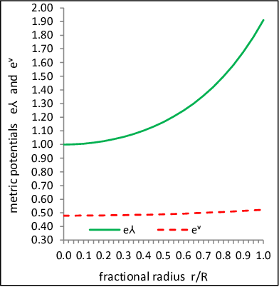
The solution should be free from physical and geometrical singularities i.e. pressure and energy density at the centre should be finite and metric potentials and should have non-zero positive values in the range . At origin Eq. (16) provides whereas from Eq. (31) we obtain . So it is clear that metric potentials are positive and finite at the centre (Fig. 1).
5.1.2 Case 2
The density and radial pressure and tangential pressure should be positive inside the star.


5.1.3 Case 3
The radial pressure must be vanishing at the boundary of sphere but the tangential pressure may not vanish at the boundary of the fluid sphere and may follow at . However, the radial pressure is equal to the tangential pressure at the centre of the fluid sphere.
5.1.4 Case 4
and so that pressure gradient is negative for .
5.1.5 Case 5
and so that pressure gradient is negative for .
5.1.6 Case 6
and so that density gradient is negative for .
Conditions (5.1.4) to (5.1.6) imply that pressure and density should be maximum at the centre and monotonically decreasing towards the surface (Figs. 2, 3).
5.2 Causality and Well Behaved Conditions:
5.2.1 Case 1
Inside the fluid ball the speed of sound should be less than the speed of light i.e. , i.e. both and are lies between 0 and 1 which can be observed from Fig. 4 as well as from Table 1.
5.2.2 Case 2
The velocity of sound monotonically decreasing away from the centre and it is increasing with the increase of density i.e. or and or for (see Fig. 4). In this context it is worth mentioning that the equation of state at ultra-high distribution has the property that the sound speed is decreasing outwards [77].

| 0.0 | 1.3165 | 1.3165 | 20.7045 | 0.9999 | 0.9394 |
|---|---|---|---|---|---|
| 0.1 | 1.3009 | 1.3044 | 20.6724 | 0.9979 | 0.9374 |
| 0.2 | 1.2543 | 1.2683 | 20.5763 | 0.9918 | 0.9312 |
| 0.3 | 1.1776 | 1.2092 | 20.4164 | 0.9819 | 0.9211 |
| 0.4 | 1.0723 | 1.1285 | 20.1933 | 0.9680 | 0.9070 |
| 0.5 | 0.9406 | 1.0285 | 19.9076 | 0.9504 | 0.8890 |
| 0.6 | 0.7852 | 0.9117 | 19.5603 | 0.9292 | 0.8672 |
| 0.7 | 0.6093 | 0.7815 | 19.1526 | 0.9044 | 0.8417 |
| 0.8 | 0.4167 | 0.6417 | 18.6860 | 0.8761 | 0.8125 |
| 0.9 | 0.2120 | 0.4967 | 18.1624 | 0.8444 | 0.7795 |
| 1.0 | 0.0000 | 0.3515 | 17.5839 | 0.8092 | 0.7427 |
5.2.3 Case 3
The ratios of the pressure to density, and (as can easily be obtained from Table 1), should be monotonically decreasing with the increase of , i.e. and , and . Then and are negative valued function for . These behaviour can be observed from Fig. 5. Also note from Table 1 which indicates the ratios via the data of , and .

5.3 Energy Conditions
A physically reasonable energy-momentum tensor has to obey the following energy conditions [78]:

, , , and
| 0.0 | 0.001861201 | 0.001979549 | 0.001979549 | 0.002216246 |
|---|---|---|---|---|
| 0.1 | 0.001858755 | 0.001975725 | 0.001976041 | 0.002210297 |
| 0.2 | 0.001851417 | 0.001964274 | 0.001965539 | 0.002192519 |
| 0.3 | 0.001839186 | 0.001945266 | 0.001948116 | 0.002163126 |
| 0.4 | 0.001822059 | 0.001918816 | 0.001923889 | 0.002122476 |
| 0.5 | 0.001800038 | 0.001885088 | 0.001893032 | 0.002071076 |
| 0.6 | 0.001773127 | 0.001844301 | 0.001855771 | 0.002009588 |
| 0.7 | 0.001741340 | 0.001796733 | 0.001812391 | 0.001938834 |
| 0.8 | 0.001704704 | 0.001742723 | 0.001763243 | 0.001859801 |
| 0.9 | 0.001663260 | 0.001682676 | 0.001708746 | 0.001773648 |
| 1.0 | 0.001617073 | 0.001617073 | 0.001649394 | 0.001681715 |
Now we check whether all the energy conditions are satisfied or not. For this purpose, numerical values of these energy conditions are given in Table 2 and accordingly their behaviour are shown in Fig. 6. This figure indicates that in our model all the energy conditions are satisfied through out the interior region.
5.4 Stability of the Stellar Models
5.4.1 Method 1
In order to have an equilibrium configuration the matter must be stable against the collapse of local regions. This requires, Le Chatelier’s principle also known as local or microscopic stability condition, that the radial pressure must be a monotonically non-decreasing function of [79].
With the energy momentum tensor of the form (3), the relativistic first law of thermodynamics may be expressed as
| (53) |
where is the radial pressure, is the total energy density and is that part of the mass density which satisfies a continuity equation and is therefore conserved throughout the motion.
We let the pressure change with density as
| (54) |
From above Eq. (54) we have
| (55) |
| (56) |
where is a parameter called the adiabatic index. A material obeying these equations is stable to gravitational collapse if the pressure times the surface area increases more rapidly than . Because the density is proportional to , the force exerted by the pressure is proportional to . This force increases more rapidly than the gravitational force when .

The later condition is, however, necessary but not sufficient to obtain a dynamically stable model [80]. Heintzmann and Hillebrandt [81] also proposed that neutron star with anisotropic equation of state are stable for . Also it is well known that Newton’s theory of gravitation has no upper mass limit if the equation of state has an adiabatic index .
The behavior of adiabatic index () is shown in Fig. 7. It is clear from figure that the value of is more than . So our model is stable.
5.4.2 Method 2
For this case let us write the generalized Tolman-Oppenheimer-Volkoff (TOV) equation in the following form:
| (57) |
where is the gravitational mass within the radius and is given by
| (58) |
Substituting the value of in above equation we get
| (59) |
The above TOV equation describes the equilibrium condition for a charged anisotropic fluid subject to gravitational (), hydrostatic (), electric () and anisotropic stress () so that:
| (60) |
where
| (61) |
| (62) |
| (63) |
| (64) |
Now, the above forces can be expressed in the explicit forms as follows:
| (65) |
| (66) |
| (67) |
| (68) |
with as mentioned earlier also.

We have shown the plot for TOV equation in Fig. 8. From the figure it is observed that the system is in static equilibrium under four different forces, e.g. gravitational, hydrostatic, electric and anisotropic to attain overall equilibrium. However, strong gravitational force is counter balanced jointly by hydrostatic and anisotropic forces. The electric force seems has negligible effect in this balancing mechanism.
5.4.3 Method 3
In our anisotropic model, to verify stability we plot the radial () and transverse () sound speeds in Fig. 9. It is observed that these parameters satisfy the inequalities and everywhere within the stellar object which obeys the anisotropic fluid models [82, 83].


Again, to check whether local anisotropic matter distribution is stable or not, we use the proposal of Herrera [82], known as cracking (or overturning) concept, which states that the potentially stable region is that one where radial speed of sound is greater than the transverse speed of sound. From the left panel of Fig. 10, we can easily say that . Since, and , therefore, as can be seen from the right panel of Fig 10. Hence, we can conclude that our compact star model provides stable configuration.
5.5 Electric charge
From the present model it is observed that in the unit of Coulomb, the charge on the boundary is C and at the centre it is as usual zero. In the Table 3 we have put the data for charge in the relativistic unit Km. However, to convert these values in Coulomb one has to multiply every value by a factor . Graphical plot is shown in Fig. 11 where charge profile is such that starting from a minimum it acquires maximum value at the boundary.
, , , . The related plots are shown
respectively in Figs. 11, 12 and 13
| (Km) | |||
|---|---|---|---|
| 0.0 | 0 | 0 | 0.4437 |
| 0.1 | 0.0035 | 0.4431 | |
| 0.2 | 0.0141 | 0.4413 | |
| 0.3 | 0.0316 | 0.4383 | |
| 0.4 | 0.0562 | 0.4341 | |
| 0.5 | 0.0879 | 0.4287 | |
| 0.6 | 0.1265 | 0.4220 | |
| 0.7 | 0.1722 | 0.4141 | |
| 0.8 | 0.2249 | 0.4049 | |
| 0.9 | 0.2847 | 0.3944 | |
| 1.0 | 0.3515 | 0.3826 |

Let us now justify this feature of charge from the available literature. It is shown by Varela et al. [38] that spheres with vanishing net charge contain fluid elements with unbounded proper charge density located at the fluid-vacuum interface and net charges can be huge ( C). On the other hand, Ray et al. [18] have analyzed the effect of charge in compact stars considering the limit of the maximum amount of charge they can hold and shown through numerical calculation that the global balance of the forces allows a huge charge ( Coulomb) to be present in a neutron star. Thus we see that the net amount of charge has less effect to balance the mechanism of the force in our model.
5.6 Pressure Anisotropy
For the present model we calculate the measure of pressure anisotropy as follows:
| (69) |
It is in general argued that the ‘anisotropy’ will be directed outward for the condition i.e. , and inward for the condition i.e. . This special feature can be observed from Fig. 12 related to our model. This kind of repulsive ‘anisotropic’ force allows for construction of a more massive compact stellar configuration [84].
One can also calculate variation of the radial and transverse pressures which are respectively given by , as can be obtained from Eq. (20), and .

5.7 Surface redshift
The effective gravitational mass in terms of the energy density can be written as
| (70) |
where is given by Eq. (46).
One can therefore provide the compactness of the star as
| (71) |
Again we define the surface redshift corresponding to the above compactness factor as follows:
| (72) |

We plot redshift in Fig. 13 from which it is evident that it is showing a gradual decrease. This feature also can be observed from the Table 3. The maximum surface redshift for the present stellar configuration of radius km turns out to be .
In this connection it is to mention that for isotropic case and in the absence of the cosmological constant the surface redshift is constraint as [85, 86, 87]. Again for an anisotropic star in the presence of a cosmological constant the constraint on surface redshift is [88] whereas Ivanov [14] put the bound . Based on the above discussion we therefore conclude that for an anisotropic star without cosmological constant the value for our model is in good agreement.
6 Some Case Studies: Comparison of Present Stellar Model with Compact Stars
6.1 Allowable Mass to Radius Ratio
Buchdahl [85] has proposed an absolute constraint of the maximally allowable mass-to-radius ratio for isotropic fluid spheres of the form (in the unit, ) which states that for a given radius a static isotropic fluid sphere cannot be arbitrarily massive. Böhmer and Harko [87] proved that for a compact object with charge, , there is a lower bound for the mass-radius ratio
| (73) |
Upper bound of the mass of charged sphere was generalized by Andréasson [89] and proved that
| (74) |

By substituting the following data, mass Solar mass and radius Km, we find out that and also which satisfy Buchdahl condition of stable configuration [85]. We also note from Fig. 14 and Table 4 that the charged stars have large mass and radius as we should expect due to the effect of the repulsive Coulomb force with the ratio increasing with charge [18]. However, unlike Ray et al. [18] where in the limit of the maximum charge the mass goes up to , which is much higher than the maximum mass allowed for a neutral compact star, our model seems very satisfactory.
, , and
| 0.7350 | 0.0085 | 0.8889 | |
| 1.0379 | 0.0169 | 0.8889 | |
| 1.2693 | 0.0252 | 0.8889 | |
| 1.4635 | 0.0334 | 0.8889 | |
| 3.1974 | 0.1549 | 0.8889 | |
| 4.3975 | 0.2819 | 0.8889 | |
| 5.2445 | 0.3847 | 0.8889 | |
| 5.5925 | 0.4280 | 0.8889 | |
| 5.7525 | 0.4479 | 0.8889 | |
| 5.9043 | 0.4665 | 0.8889 | |
| 6.0000 | 0.4760 | 0.8889 |
6.2 Validity with Strange Star Candidates
We have presented two tables here (Tables 5 and 6) from where it can be observed that the mass and radius are exactly correspond to the strange stars and . What we did in the tables are as follows: by considering the mass and radius of the above mentioned stars we have figured out data for the model parameters, and in the next step we evaluated data for different physical parameters, e.g. central density, surface density and central pressure, of those strange stars. One can observe that these data set are in good agreement with the available observational data.
In this connection we would like to mention that previously Gupta and Maurya [90] showed a similar result for with isotropic fluid distribution and charge generalization of Durgapal [66]. We also note that like the models offered by Kalam et al. [42], Hossein et al. [84] and Kalam et al. [91] our presented models provide significantly promising results with observational evidences.
| Strange star | |||||||||||
|---|---|---|---|---|---|---|---|---|---|---|---|
| candidates | () | (Km) | |||||||||
| 0.9693 | 6.0 | 1.1426 | 0.4798 | 5 | 11 | 1 | 0.25 | 0.11 | 4.2395 | ||
| 0.88 | 7.7 | 1.7518 | 0.6217 | 4 | 14 | 1 | 0.16 | 0.13 | 2.1546 |
for the above parameter values of Table 1
| Strange star | Central Density | Surface density | Central pressure |
|---|---|---|---|
| candidates | () | () | () |
7 Conclusion
In this work we have presented a set of new solutions for an anisotropic charged fluid distribution under the framework of General Theory of Relativity. To solve the Einstein-Maxwell field equations we construct a general algorithm for all possible anisotropic charged fluid spheres. As an additional condition which simplifies the physical system of space-time we consider a special source function in terms of metric potential . We further adopt exterior solution of Reissner-Nordström so that our interior solution can be matched smoothly as a consequence of junction conditions at the surface of spheres .
The solutions set thus obtained exhibits regular physical behaviour as can be observed from figures and tables on different parameters. We specifically discuss (i) regularity and reality conditions (applied for metric potentials and , energy density , fluid pressures and , pressure gradients and , and density gradient ), and (ii) causality and well behaved conditions (applied for speed of sound and ratios of pressure to densities and ). Beside all these general physical properties the solutions set shows desirable and essential features for energy condition, stability condition, charge distribution, pressure anisotropy and surface redshift. Among these physical parameters as a special case, regarding electric charge distribution of our model, we note that the charge on the boundary is Coulomb and at the centre it is as usual zero. Other features of charge is also available in the literature [18, 38, 65] in connection to stable configuration of compact stars where it has been shown that the global balance of the forces allows a huge charge ( Coulomb) to be present in a neutron star.
We also observe some special and interesting features for our stellar models which are related to compact stars as follows:
(1) Allowable mass to radius ratio: The condition of Buchdahl [85] related to the maximally allowable mass-to-radius ratio for isotropic fluid spheres is of the form . By substituting the following data, mass and radius Km, we find out that which satisfies Buchdahl condition of stable configuration [85] as mentioned above.
(2) Validity with strange stars: We have prepared several data set from where it is observed that the mass and radius are exactly correspond to the strange stars and . Therefore, one can note that like the models of Kalam et al. [42], Hossein et al. [84] and Kalam et al. [91] our models also provide significantly promising results with observational evidences.
In this work we have studied the case for only in the source function because of the fact that this value is more relevant for exploring existence and properties of strange stars. There is however scope for further study with other values of also as follows: (1) For integer values of (not possible for all other positive integer values), and (2) For fractional values of there are two possibilities: (i) If lies between and then exact solutions are possible for all fractional values, and (ii) If is greater than then for all fractional values of except the values of and , where is a positive integer ( and ). However, the specific value is not allowed for these factors to study the solutions for the present model.
As a final comment we would like to mention that Tiwari and Ray [92] proved that any relativistic solution for spherically symmetric charged fluid sphere has electromagnetic origin and hence provides Electromagnetic Mass model [93, 94, 95, 96]. Therefore, it would be an interesting task to verify whether our model also represents an electromagnetic mass or not and can be studied elsewhere in a future project.
Appendix
with where in the table is a positive integer
| n | Electric charge function | Pressure anisotropy | Behavior of | Reference |
| () | ||||
| 1 | 0 | 0 | No | [47] |
| 1 | Kx | 0 | Yes | [97] |
| 2 | 0 | 0 | No | [69, 71] |
| 1,2,7 | 0 | Yes | [97] | |
| 2 | 0 | Yes | [98] | |
| 2 | 0 | Yes | [99] | |
| 2 | 0 | Yes | [99] | |
| 2 | 0 | Yes | [99] | |
| 2 | Yes | [65] | ||
| 3 | 0 | Yes | [100] | |
| 4 | 0 | Yes | [101] | |
| 5 | 0 | Yes | [102] | |
| 6 | 0 | Yes | [103] | |
| n | 0 | 0 | Yes () | [62] |
| n | 0 | Yes () | [104] | |
| n | 0 | Yes () | [105] | |
| n | Yes | [106] | ||
Acknowledgement
SKM acknowledges support from the Authority of University of Nizwa, Nizwa, Sultanate of Oman. Also the author SR is thankful to the authority of Inter-University Centre for Astronomy and Astrophysics, Pune, India for providing him Associateship programme under which a part of this work was carried out.
References
- (1) S. Rosseland, Mon. Not. R. Astron. Soc. 84, 720 (1924).
- (2) L. Neslusan, Astron. Astrophys. 372, 913 (2001).
- (3) P. Anninos, T. Rothman, Phys. Rev. D 65, 024003 (2001).
- (4) A. Giuliani, T. Rothman, Gen. Relativ. Gravit. 40, 1427 (2008).
- (5) S. Datta Majumdar, Phys. Rev. D 72, 390 (1947).
- (6) A. Papapetrou, Proc. R. Irish Acad. 81, 191 (1947).
- (7) W.B. Bonnor, S.B.P. Wickramasuriya, Mon. Not. R. Astron. Soc. 170, 643 (1975).
- (8) J.D. Bekenstein, Phys. Rev. D 4, 2185 (1971).
- (9) J.L. Zhang, W.Y. Chau, T.Y. Deng, Astrophys. Space Sci. 88, 81 (1982).
- (10) F. de Felice, Y. Yu, Z. Fang, Mon. Not. R. Astron. Soc. 277, L17 (1995).
- (11) F. de Felice, S.M. Liu, Y.Q. Yu, Class. Quantum Gravit. 16, 2669 (1999).
- (12) Y.Q. Yu, S.M. Liu, Comm. Theor. Phys. 33, 571 (2000).
- (13) N.K. Glendenning, Compact Stars: Nuclear Physics, Particle Physics, and General Relativity (Springer-Verlag, 2000).
- (14) B.V. Ivanov, Phys. Rev. D 65, 104001 (2002).
- (15) A. Treves, R. Turolla, Astrophys. J. 517, 396 (1999).
- (16) S. Ray, B. Das, Astrophys. Space Sci. 282, 635 (2002).
- (17) S. Ray, B. Das, Mon. Not. R. Astron. Soc. 349, 1331 (2004).
- (18) S. Ray, A.L. Espindola, M. Malheiro, J.P.S. Lemos, V.T. Zanchin, Phys. Rev. D 68, 084004 (2003).
- (19) D. Horvat, S. Ilijić, A. Marunović, Class. Quantum Gravit. 26, 025003 (2009).
- (20) S. Thirukkanesh, S.D. Maharaj, Class. Quantum Gravit. 25, 235001 (2008).
- (21) R. Stettner, Ann. Phys. 80, 212 (1973).
- (22) F. Rahaman, S. Ray, A.K. Jafry, K. Chakraborty, Phys. Rev. D 82, 104055 (2010).
- (23) R. Sharma, S. Mukherjee, S.D. Maharaj, Gen. Relativ. Gravit. 33, 999 (2001).
- (24) F. de Felice, Y. Yu, J. Fang, Mon. Not. R. Astron. Soc. 277, L17 (1995).
- (25) S. Chandrasekhar, Astrophys. J. 74, 81 (1931).
- (26) E. Witten, Phys. Rev. D 30, 272 (1984).
- (27) N.K. Glendenning, Compact Stars: Nuclear physics, particle physics and general relativity (Springer 1997).
- (28) R.X. Xu, Acta Astron. Sinica 44, 245 (2003).
- (29) F. DePaolis et al., Int. J. Mod. Phys. D 16, 827 (2007).
- (30) K.S. Cheng, Z.G. Dai, Phys. Rev. Lett. 77, 1210 (1996).
- (31) K.S. Cheng, Z.G. Dai, Phys. Rev. Lett. 80, 18 (1998).
- (32) X.-D. Li, I. Bombaci, M. Dey, J. Dey, E.P.J. van den Heuvel, Phys. Rev. Lett. 83, 3776 (1999).
- (33) R. Ruderman, Ann. Rev. Astron. Astrophys. 10, 427 (1972).
- (34) R. Bowers, E. Liang, Astrophys. J. 188, 657 (1974).
- (35) M.K. Mak, T. Harko, Proc. R. Soc. Lond. A 459, 393 (2002).
- (36) M.K. Mak, T. Harko, Proc. R. Soc. A 459, 393 (2003).
- (37) V.V. Usov, Phys. Rev. D 70, 067301 (2004).
- (38) V. Varela, F. Rahaman, S. Ray, K. Chakraborty, M. Kalam, Phys. Rev. D 82, 044052 (2010).
- (39) F. Rahaman, S. Ray, A.K. Jafry, K. Chakraborty, Phys. Rev. D 82, 104055 (2010).
- (40) F. Rahaman, P.K.F. Kuhfittig, M. Kalam, A.A. Usmani, S. Ray, Class. Quantum Gravit. 28, 155021 (2011).
- (41) F. Rahaman, R. Maulick , A.K. Yadav, S. Ray, R. Sharma, Gen. Relativ. Gravit. 44, 107 (2012).
- (42) M. Kalam, F. Rahaman, S. Ray, Sk.M. Hossein, I. Karar, J. Naskar, Eur. Phys. J. C 72, 2248 (2012).
- (43) M.K. Mak, T. Harko, Phys. Rev. D 70, 024010 (2004); Int. J. Mod. Phys. D. 13, 149 (2004).
- (44) K. Lake, Phys. Rev. D 67, 104015 (2003).
- (45) K. Lake, Phys. Rev. Lett. 92, 051101 (2004).
- (46) L. Herrera, J. Ospino, A. Di Parisco, Phys. Rev. D 77, 027502 (2008).
- (47) R.C. Tolman, Phys. Rev. 55, 364 (1939).
- (48) J.R. Oppenheimer, G.M. Volkoff, Phys. Rev. 55, 374 (1939).
- (49) D.D. Dionysiou, Astrophys. Space Sci. 85, 331 (1982).
- (50) P.S. Florides, J. Phys. A, Math. Gen. 16, 1419 (1983).
- (51) L. Herrera, J. Ponce de Leon, J. Math. Phys. 26, 2302 (1985).
- (52) M.K. Gokhroo, A.L. Mehra, Gen. Relativ. Gravit. 26, 75 (1994).
- (53) A.S. Berger, R. Hojman, J. Santamarina, J. Math. Phys. 28, 2949 (1987).
- (54) T.W. Baumgarte, A.D. Rendall, Class. Quantum Gravit. 10, 327 (1993).
- (55) M. Mars, M. Merc Martn-Prats, J.M.M. Senovilla, Phys. Lett. A 218, 147 (1996).
- (56) S.K. Maurya, Y.K. Gupta, Nonlinear Analysis: Real World Applications 13, 677 (2012).
- (57) S.K. Maurya, Y.K. Gupta, B. Dayanandan, T.T. Smitha, Astrophys. Space Sci. 356, 75 (2014).
- (58) M.C. Durgapal, A.K. Pande, Astrophys. space Sci. 102, 49 (1984).
- (59) M. Ishak, L. Chamandy, N. Neary, K. Lake, Phys. Rev. D 64, 024005 (2001).
- (60) N. Pant, Astrophys. Space Sci. 331, 633 (2011).
- (61) S.K. Maurya, Y.K. Gupta, Pratibha, Int J Theor Phys 51, 943 (2012).
- (62) S.K. Maurya, Y.K. Gupta, Astrophys Space Sci. 334, 145 (2011).
- (63) S.K. Maurya, Y.K. Gupta, Astrophys Space Sci. 337, 151 (2012).
- (64) S.K. Maurya, Y.K. Gupta, Astrophys. Space Sci. 344, 243 (2013).
- (65) M.H. Murad, S. Fatema, Eur. Phys. J C 75, 533 (2015).
- (66) M.C. Durgapal, R.S. Fuloria, Gen. Relativ. Gravit. 17, 671 (1985).
- (67) M.S.R. Delgaty, K. Lake, Comput. Phys. Commun. 115, 395 (1998).
- (68) S.K. Maurya, Y.K. Gupta, M.K. Jasim, Astrophys. Space Sci. 355, 2171 (2014).
- (69) M. Wyman, Phys. Rev. 75, 1930 (1949).
- (70) B. Kuchowicz, Astrophys. Space Sci. 33, L13 (1975).
- (71) R.J. Adler, J. Math. Phys. 15, 727 (1974).
- (72) R.C. Adams, J.M. Cohen, Astrophys. J. 198, 507 (1975).
- (73) H. Heintzmann, Z. Phys. 228, 489 (1969).
- (74) M.C. Durgapal, J. Phys. A 15, 2637 (1982).
- (75) C.W. Misner, D.H. Sharp, Phys. Rev. B 136, 571 (1964).
- (76) L. Herrera, N.O. Santos, Phys. Rep. 286, 53 (1997).
- (77) V. Canuto, In: Solvay Conference on Astrophysics and Gravitation (Brussels, 1973).
- (78) M. Visser, Lorentzian wormholes (Springer, Chap. 12, 1996).
- (79) S.S. Bayin, Phys. Rev. D 26, 1262 (1982).
- (80) B.O.J. Tupper, Gen. Relativ. Gravit. 15, 47 (1983).
- (81) H. Heintzmann, W. Hillebrandt, Astron. Astrophys. 38, 51 (1975).
- (82) L. Herrera, Phys. Lett. A, 165 206 (1992).
- (83) H. Abreu, H. Hernández, L. A. Núnez, Class. Quantum Gravit. 24, 4631 (2007).
- (84) Sk.M. Hossein, F. Rahaman, J. Naskar, M. Kalam, S. Ray, Int. J. Mod. Phys. D, 21, 1250088 (2012).
- (85) H.A. Buchdahl, Phys. Rev. 116, 1027 (1959).
- (86) N. Straumann, General Relativity and Relativistic Astrophysics (Springer Verlag, Berlin, 1984).
- (87) C.G. Böhmer, T. Harko, Gen. Relativ. Gravit. 39, 757 (2007).
- (88) C.G. Böhmer, T. Harko, Class. Quantum Gravit. 23, 6479 (2006).
- (89) H. Andréasson, Commun. Math. Phys. 288, 715 (2009).
- (90) Y.K. Gupta, S.K. Maurya, Astrophys. Space Sci. 331, 135 (2011).
- (91) M. Kalam, F. Rahaman, Sk. M. Hossein, S. Ray, Euro. Phys. J. C 72, 2248 (2012).
- (92) R.N. Tiwari, S. Ray, Astrophys. Space Sci. 180, 143 (1991).
- (93) H.A. Lorentz, Proc. Acad. Sci. Amsterdam 6 (1904) (Reprinted in: Einstein et al., The Principle of Relativity (Dover, INC, p. 24, 1952)).
- (94) J.A. Wheeler, Geometrodynamics (Academic, New York, p. 25, 1962).
- (95) R.P. Feynman, R.B. Leighton, M. Sands, The Feynman Lectures on Physics (Addison-Wesley, Palo Alto, Vol. II, Chap. 28, 1964).
- (96) F. Wilczek, Phys. Today 52, 11 (1999).
- (97) N. Pant, S. Rajasekhara, Astrophys Space Sci. 333, 161 (2011).
- (98) S. Fatema, M.H. Murad, Int. J. Theor. Phys. 52, 2508 (2013).
- (99) M.H. Murad, S. Fatema, Int. J. Theor. Phys. 52, 4342 (2013).
- (100) N. Pant, S.K. Maurya, Appl. Math. Comput. 218, 8260 (2012).
- (101) S.K. Maurya, Y.K. Gupta, Pratibha, Int. J. Mod. Phys. D 20, 1289 (2011).
- (102) Y.K. Gupta, S.K. Maurya, Astrophys. Space Sci. 332, 155 (2011).
- (103) S.K. Maurya, Y.K. Gupta, Astrophys. Space Sci. 332, 481 (2011).
- (104) S.K. Maurya, Y.K. Gupta, Astrophys. Space Sci. 334, 301 (2011).
- (105) S.K. Maurya, Y.K. Gupta, Phys. Scr. 86, 025009 (2012)
- (106) S.K. Maurya, Y.K. Gupta, Astrophys Space Sci. 353, 657 (2014).