Scattering of matter-waves in spatially inhomogeneous environments
Abstract
We study scattering of quasi one-dimensional matter-waves at an interface of two spatial domains, one with repulsive and one with attractive interatomic interactions. It is shown that the incidence of a Gaussian wavepacket from the repulsive to the attractive region gives rise to generation of a soliton train. More specifically, the number of emergent solitons can be controlled e.g. by the variation of the amplitude or the width of the incoming wavepacket. Furthermore, we study the reflectivity of a soliton incident from the attractive region to the repulsive one. We find the reflection coefficient numerically and employ analytical methods, that treat the soliton as a particle (for moderate and large amplitudes) or a quasi-linear wavepacket (for small amplitudes), to determine the critical soliton momentum – as function of the soliton amplitude – for which total reflection is observed.
pacs
03.75.Kk, 03.75.LmI Introduction
For almost two decades, the study of nonlinear phenomena occurring in atomic Bose-Einstein condensates has experienced an enormous increase of interest [1, 2]. A prominent example, in the quasi one-dimensional (1D) setting, is the experimental observation of robust matter-wave solitons of the bright [3] and dark [4] type, and the study of their properties (see, e.g., the reviews [5] and [6] for bright and dark solitons, respectively). Such coherent nonlinear excitations of BECs are also interesting from the viewpoint of potential applications, ranging from coherent matter-wave optics to precision measurements and quantum information processing. Indeed, the formal similarities between nonlinear and matter-wave optics [7] indicate that coherent matter-waves may in principle be controlled similarly to their optical siblings in optical fibers, waveguides, photonic crystals, and so on [8].
In that respect, it is not surprising that there exist many works devoted to the manipulation of matter waves. Among various techniques that have been proposed, an experimentally tractable one refers to engineering the “environment” of the matter-wave, by magnetically [9] or optically [10] induced Feshbach resonances, which makes it possible to control the effective nonlinearity in the condensate. The application of such a “Feshbach resonance management” (FRM) technique [11] in the temporal domain was used for the realization of matter-wave bright solitons by switching the interatomic interactions from repulsive to attractive [3]; it was also proposed as a means to stabilize attractive higher-dimensional BECs against collapse [12, 13] and to create robust quasi-1D matter-wave breathers [11, 14]. On the other hand, the FRM technique in the spatial domain, which gives rise to the so-called “collisionally inhomogeneous condensates” [15] with a spatially modulated nonlinearity, has also been extensively studied. In particular, novel phenomena and a variety of applications have been proposed in this context, including the adiabatic compression of matter-waves [15, 16], Bloch oscillations of matter-wave solitons [15], atomic soliton emission and atom lasers [17], enhancement of transmittivity of matter waves through barriers [18], formation of stable condensates exhibiting both attractive and repulsive interatomic interactions [19], solitons in combined linear and nolinear potentials [20], generation of solitons [21] and vortex rings [22], control of Faraday waves [23], and many others. A detailed recent review of such inhomogeneously nonlinear settings, especially in the context of periodic (i.e., nonlinear lattice) variations can be found in [24].
In this work, we study the scattering of matter-waves in a collisionally inhomogeneous environment. In particular, we consider a quasi-1D setting (whereby matter waves are oriented along the -direction) and assume that the scattering length is piecewise constant for and , taking respectively the values and , and changes sign at . In other words, we assume that the normalized scattering length takes the form:
| (1) |
where is the spatial scale over which the transition from the asymptotic values and takes place. For the above setting, and in the framework of the mean-field approximation, we will investigate two different scattering processes; a description of our considerations and the organization of the paper are as follows.
First, in Section II, we study the incidence of a nearly linear (Gaussian) wavepacket from the repulsive region () to the attractive region (), and demonstrate the generation of a train of bright solitons. By numerically integrating the pertinent Gross-Pitaevskii (GP) equation, we determine the number of created solitons as functions of the initial data (amplitude, width and momentum of the incident wavepacket), as well as the difference of the values of the scattering length.
In Section III, we study the reflectivity of a bright soliton from the scattering length interface; the soliton is assumed to exist and travel from the attractive region () towards the repulsive region (). We find numerically the reflection coefficient as a function of the soliton momentum and amplitude, and find that it has a step-like dependence on momentum for sufficiently weak solitons. In the case of total reflection, we use an analytical approximation (treating the soliton as a particle) and find the equation of motion for the soliton center. This equation is used to determine the critical value of momentum below which total reflection occurs, which turns out to depend linearly on the soliton amplitude. Additionally, for extremely weak solitons, employing results from linear quantum mechanics [25], we also find a (different) linear dependence of the critical momentum on the soliton amplitude. Both analytical estimates, for weak and strong solitons are found to be in very good agreement with the numerical results, with the latter also encompassing a transition region between the two regimes.
Finally, Section IV concludes our findings and presents a number of directions for future study.
II Reflectivity of a Gaussian wavepacket from the scattering length interface
II.1 Model and creation of a soliton train
Our considerations start from the following Gross-Pitaevskii (GP) equation, which describes a quasi-1D BEC oriented along the -axis [1, 2]:
| (2) |
Here is the mean-field order parameter, is the atomic mass, is the transverse confining frequency, and the s-wave scattering length [ () corresponds to repulsive (attractive) interatomic interactions]. Considering a situation where proper spatially dependent fields close to Feshbach resonances are employed, we assume that the scattering length is piecewise constant for and , taking the form
| (3) |
where is the spatial scale over which the transition from the asymptotic value (for ) to (for ) takes place.
A strategy for developing a corresponding experimental implementation can be based on the interaction tunability of specific atomic species by applying external magnetic fields. For example, for cesium the s-wave scattering length changes sign through a zero-crossing at an external field strength of 17 G [26]. Confining cesium atoms in an elongated trapping potential near the surface of an atom chip [27] will allow for appropriate local engineering of to form steps of varying widths , where the atom-surface separation sets a scale for achievable minimum step widths. The trapping potential can be formed optically, possibly also by a suitable combination of optical and magnetic fields, whereby care has to be taken as the magnetic field will influence both the external potential and the scattering length profile ; see e.g. the relevant discussion of [28].
Normalizing time and space in Eq. (2), as and (where is the transverse harmonic oscillator length), as well as the density as , we cast Eq. (2) into the following dimensionless form:
| (4) |
where the function is given by Eq. (1). For our analytical and numerical considerations below, we will use the values , and corresponding to an abrupt, step-like transition.
It is relevant to point out here that, generally, Eq. (2) as well as its variants attempting to more adequately capture transverse degrees of freedom (see the quasi-1D models of Refs. [29] and [30]), suggest that the variations/modulations in transverse trapping strength can be used in a way equivalent to longitudinal variations of the scattering length. This idea has been used even in a quantitative fashion, e.g., to explain the phenomenology of the formation of Faraday wave patterns – cf. Ref. [31] (and relevant work in Ref. [23]). Nevertheless, this type of consideration is not applicable in the present setting, given the sign changing nature of the nonlinearity.
We now assume that a Gaussian wavepacket of amplitude and width , initially located at (i.e., in the repulsive region), moves towards the attractive region. The specific form of the wavepacket, which is used as an initial condition for Eq. (4) in our simulations, is:
| (5) |
where is the initial momentum of the wavepacket. Notice that this form of the wavepacket approximates the ground state profile in the case of relatively small atom numbers (corresponding to a weak nonlinearity).

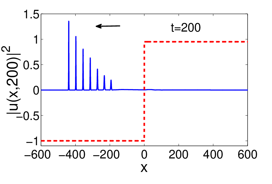

Using the parameter values , , and (as well as , and ), we depict the corresponding configuration in the top panel of Fig. 1. In the middle and bottom panels of the same figure, we show the subsequent dynamics: it is observed that the wavepacket is transmitted through the discontinuity of the scattering length at and, after entering the region with attractive interactions, it transforms into a train of bright solitons. Notice that the soliton generation process is such that each generated soliton is larger than the one that will be generated at a later time. This is due to the fact that once a portion of the condensate enters the attractive side and is self-organized into a soliton, the number of atoms of the wavepacket on the repulsive side is decreased and, thus, a smaller soliton will be generated next. It is interesting to observe that the ratio of the velocities of two adjacent solitons in the train is constant; as a result, for each certain time instance, the distance between adjacent solitons is the same. Note that the results on the generation – and characteristics – of the atomic soliton train described above are reminiscent to the ones found in Ref. [17], but by means of a somewhat different physical mechanism: in that work, the soliton train was produced via a sufficiently deep spatially-dependent nonlinearity which acted on a trapped Gaussian wavepacket (existing between a region of vanishing and that of negative scattering length). The depth of the (abrupt) negative step was found to control the number of emitted solitary waves.
We find that the number of the created solitons, , depends on the momentum , the amplitude and the width of the Gaussian wavepacket, as well as the height of the interface . Results pertaining to the count of the soliton number are shown in Fig. 2: larger initial amplitudes and/or widths of the wavepacket result in a larger number of solitons. On the other hand, increasing the initial momentum and/or the height of the interface the number of solitons seems to have a weaker effect on the process; for the particular example shown in Fig. 1, the number of solitons is at time . Here, we should note that for the counting of the number of solitons, we have included only solitons of amplitudes at least of the first created soliton.

III Reflectivity of a soliton from the scattering length interface
Next, we consider the reflectivity of a bright soliton at the scattering length interface. We assume, in particular, that a bright soliton moves from the attractive () to the repulsive region () and is, thus, scattered at the interface, at , caused by the change of the sign of the nonlinearity. This dynamical scenario is, effectively, complementary to the one studied in Section II.

The bright soliton propagating in the attractive region has the form:
| (6) |
where , , and respectively denote the amplitude, velocity, initial position and frequency of the soliton. Then, we numerically integrate Eq. (2) with the initial condition taken as
| (7) |
and observe the dynamics of the scattering process. Typical outcomes are shown in Fig. 3; in all cases, we fix the initial soliton momentum, at , and vary the amplitude . We observe that if the soliton amplitude is sufficiently small (large) then total transmission (reflection) is found –cf. top (bottom) panel of the figure for (). On the other hand, for a moderate value of (e.g., –cf. middle panel) the soliton is partially transmitted and reflected.
The soliton reflectivity can be calculated numerically upon determining the reflection coefficient , defined as the number of atoms remaining in the (attractive) region over the number of atoms of the incident soliton. Taking into regard that the latter is given by , we can express as:
| (8) |
Here, is a time sufficiently large such that the reflected and transmitted parts of the soliton are spatially well separated; this separation is set by a spatial region of extent around and, accordingly, is appropriately chosen for each individual numerical experiment.
Figure 4 shows the reflection coefficient as a function of the initial soliton momentum (for ) and various values of the soliton amplitude . We observe that when is increased, the respective reflection coefficient curves drift towards larger momentum values and the curves become smoother: the transition from total reflection to total transmission becomes less sharp. This means that the interval of momenta for which partial transmission and reflection occur (as in the middle panel of Fig. 3) increases with increasing soliton amplitude.
From the above discussion, it is obvious that the soliton keeps its particle-like character only in the case where it is totally reflected (cf. bottom panel of Fig. 3): in the cases of total or partial transmission, the soliton is not supported in the repulsive regime and it is eventually destroyed. We can thus adapt the particle picture for the soliton dynamics in the total reflection regime, and describe analytically the soliton trajectory and its reflectivity properties. Our approach based on the center of mass (defined below) extends the corresponding considerations of Ref. [33], where a similar methodology was developed for the case of a linear step potential.

We start with the soliton’s center of mass, given by:
| (9) |
which is connected with the soliton momentum through the equation . Then, differentiating the latter expression with respect to , and using Eq. (4), it is straightforward to derive the following equation of motion for :
| (10) |
The integral on the right-hand side of Eq. (10) can be calculated in an analytical form, upon approximating [cf. Eq. (1)] by a Heavyside function in the limiting case where . Then, is approximated by a delta function, and integrating the right-hand side of Eq. (10), we end up with the following result:
| (11) |
Then, taking into regard that the soliton center is connected with the center of mass through the equation , we can express Eq. (11) as follows:
| (12) |
where the effective potential is given by:
| (13) | |||||
Equation (12) shows that the soliton can be regarded as a Newtonian unit-mass particle, which evolves in the presence of the effective potential ; the latter, has a shape of a step-like barrier, as depicted in Fig. 5. Thus, according to this particle picture, the soliton will be totally reflected if its initial energy is less than the “height” of the barrier. Since the soliton is expected to interact with the effective potential only through its exponential leading tail, the soliton center is anticipated to never reach the interface at , but it will approach it only up to a distance roughly equal to the half-width at half-maximum (HWHM) of the soliton; the above situation is schematically illustrated in Fig. 5. Thus, taking into regard that the soliton’s HWHM, denoted by , is connected with the inverse width through the equation , we can find that the relevant barrier height is given by , where is the initial soliton position. According to the above arguments, the soliton will be totally reflected if the initial soliton energy is less than (or equal to) the effective barrier height, namely:
| (14) |

We have numerically checked the validity of this analysis by comparing, at first, the numerically obtained soliton trajectory [by means of direct numerical integration of Eq. (4) in the case of total reflection] with the approximate analytical result of Eq. (12). A typical example, corresponding to a soliton amplitude and momentum , is shown in Fig. 6. There, the numerical result is displayed in the form of a contour plot for the evolution of the soliton density, as well as the analytical result of Eq. (12) – cf. dashed line in the figure. Note that similar results were obtained for soliton amplitudes . It can be seen that the dashed line follows with a fairly good accuracy the evolution of the soliton center. The slight discrepancy observed can be explained as follows: the tail of the bright soliton, in case of total reflection (cf. Figs. 5 and 6), interacts with the interface and enters the repulsive area, and eventually comes back to the attractive region. This effect, which cannot be explained via the particle approach, causes a slight shift in the soliton trajectory. Thus, the trajectory obtained from Eq. (10) has naturally a slight discrepancy for any soliton amplitude .

Next, employing Eq. (14), it is possible to derive analytically the critical value of the initial momentum [when the equality in Eq. (14) holds], for which total reflection occurs, as a function of the soliton amplitude and the parameters characterizing the scattering length profile. The result is:
| (15) |
where constant and . Note that Eq. (15) suggests a linear dependence of on , which is confirmed by our numerical simulations. Indeed, as shown in Fig. 7, for solitons of sufficiently large amplitudes, i.e., for , this analytical prediction [depicted by the solid (green) straight line] is in an excellent agreement with the numerical result for [depicted by the (red) dots]. Notice that the numerically obtained values for are calculated so that the respective reflection coefficient values become less than unity by a factor of ; however, we note here that the results presented are only weakly sensitive to the selection of the particular threshold.

For weaker solitons it is expected that our analytical approximations described above should be less accurate: this is due to the fact that for small values of , the nonlinearity becomes extremely weak, and thus a linear description of the problem would be more appropriate. In such a case, the soliton can be treated as a linear wavepacket, which is scattered from an effective step barrier; the latter, is basically formed by the step-like change of the scattering length profile. Then, the reflection coefficient can be approximated from the corresponding linear problem [25] as follows:
| (16) |
where and denote, respectively, the energy of the wavepacket and the height of the effective potential barrier. Notice that Eq. (16) stands for plane waves; however, it can still provide a reasonable approximation as long as the soliton width is sufficiently large, i.e., for sufficiently weak solitons. In our case, the soliton energy is given by (see, e.g., Ref. [2]):
| (17) |
while the strength of the effective barrier potential is given by:
| (18) |
Then, total reflection, i.e., in Eq. (16), occurs for ; the latter equation leads to the following result for the critical momentum :
| (19) |
The above approximate analytical result, which is relevant to weak solitons, also shows a linear dependence of on and is in a very good agreement with the numerical results, as shown in Fig. 7 for .
In summary, we capture the regime of small by means of the linear/wave theory, and the regime of large by our soliton particle theory, while between the two we interpolate via the use of numerical computations as shown in Fig. 7.
IV Conclusions
In this work, we studied the scattering of quasi-1D matter-waves in a spatially inhomogeneous environment, characterized by a piecewise constant profile of the scattering length , such that for , for , and changes sign at . This way, in the region () the interatomic interactions are attractive (repulsive). We investigated two different dynamical scenarios:
- (i)
the scattering of a quasi-linear (Gaussian) wavepacket at the scattering length interface, with the wavepacket traveling from the repulsive to the attractive region, and
- (ii)
the scattering of a matter-wave bright soliton at the scattering length interface, with the soliton traveling from the attractive to the repulsive region.
In case (i), we found that when the wavepacket enters the attractive region it evolves into a train of bright solitons. The soliton train is such that each generated soliton is larger than the one that will be generated at later times, while the distance between adjacent solitons is the same. We counted the number of the created solitons, as a function of the wavepacket’s initial characteristics (momentum, amplitude, and width) and the height of the nonlinearity interface , and found that larger initial amplitudes and/or widths of the initial wavepacket result in a larger number of solitons.
For case (ii), we found that the incidence of the soliton at the scattering length interface generally leads to total transmission, total reflection, or partial transmission/reflection. The reflection coefficient was determined numerically as a function of the initial soliton momentum, for different soliton amplitudes. For sufficiently weak solitons, we found an almost abrupt change from total transmission to total reflection, effectively associated with the linear phenomenology in a step potential. For stronger solitons, the reflection coefficient featured a smoother dependence on the momentum.
We also developed analytical approximations – that treated the solitons as particles (for large amplitudes) or linear wavepackets (for small amplitudes) – to determine the critical value of soliton momentum, , below which total reflection occurs. We found that depends linearly on the soliton amplitude, but with different slopes in the purely nonlinear and the quasi-linear regimes. Numerically, we find a smooth crossover between these two regimes, which can be interpreted as a gradual continuous change of the soliton from being dominated by wave-like to particle-like properties. Our analytical predictions were found to be in very good agreement with the corresponding numerical results.
There are numerous directions that may be worth considering for future efforts. One of these is to consider the possibility of multiple steps and their interplay. Another is to examine the interplay of the nonlinear step with an external linear potential or with a non-trivial background (e.g. on the repulsively interacting side which can support such a background) and to explore the dynamics of incident wavepackets in such settings. Potentially, probing the soliton dynamics in such configurations could be utilized towards retrieving quantitative information about the nature of linear and/or nonlinear unknown potentials.
From a more rigorous mathematical perspective, it will be interesting to attempt to connect the present setting to the extensive developments in treating integrable problems with suitable boundary conditions (e.g. on the half line), as detailed e.g., in Ref. [34]. A way to make this connection may be to consider the GP equation e.g. solely on the attractive domain with a boundary condition inferred by the incidence of the Gaussian wavepacket at (i.e., a Gaussian in time boundary condition). A potential by-product of such a formulation might be the identification of the number of solitary waves that will emerge, as a function of the properties of this effective (and localized in time) boundary drive.
Finally, it would be of particular interest to extend considerations to the two- or higher-dimensional setting. There, understanding the properties of the formed solitons, e.g., on the attractive interaction “domain”, taking into consideration the collapse feature that arises in the critical or super-critical higher-dimensional case [35], would be especially relevant.
Acknowledgements.
The work of D.J.F. was partially supported by the Special Account for Research Grants of the University of Athens. P.G.K. acknowledges support from the National Science Foundation under grant DMS-1312856, from FP7-People under grant IRSES-605096 from the Binational (US-Israel) Science Foundation through grant 2010239, and from the US-AFOSR under grant FA9550-12-10332. P.K. acknowledges support by EPSRC (grant EP/I017828/1) and the EU. P.G.K. and P.K. also acknowledge the hospitality of the Synthetic Quantum Systems group and of Markus Oberthaler at the Kirchhoff Institute for Physics (KIP) at the University of Heidelberg, as well as that of the Center for Optical Quantum Technologies (ZOQ) and of Peter Schmelcher at the University of Hamburg, as well as of the Center for Nonlinear Studies at the Los Alamos National Laboratory. P.G.K.’s work at Los Alamos is supported in part by the U.S. Department of Energy.
References
- [1] P. G. Kevrekidis, D. J. Frantzeskakis, and R. Carretero-González (eds.), Emergent Nonlinear Phenomena in Bose-Einstein Condensates: Theory and Experiment (Springer-Verlag, Berlin, 2008).
- [2] R. Carretero-González, D. J. Frantzeskakis, and P. G. Kevrekidis, Nonlinearity 21, 139 (2008).
- [3] K. E. Strecker, G. B. Partridge, A. G. Truscott, and R. G. Hulet, Nature (London) 417, 150 (2002); L. Khaykovich, F. Schreck, G. Ferrari, T. Bourdel, J. Cubizolles, L. D. Carr, Y. Castin, and C. Salomon, Science 296, 1290 (2002); S. L. Cornish, S. T. Thompson, and C. E. Wieman, Phys. Rev. Lett. 96, 170401 (2006).
- [4] S. Burger, K. Bongs, S. Dettmer, W. Ertmer, K. Sengstock, A. Sanpera, G. V. Shlyapnikov, and M. Lewenstein, Phys. Rev. Lett. 83, 5198 (1999); J. Denschlag, J. E. Simsarian, D. L. Feder, C. W. Clark, L. A. Collins, J. Cubizolles, L. Deng, E. W. Hagley, K. Helmerson, W. P. Reinhardt, S. L. Rolston, B. I. Schneider, and W. D. Phillips, Science 287, 97 (2000); B. P. Anderson, P. C. Haljan, C. A. Regal, D. L. Feder, L. A. Collins, C. W. Clark, and E. A. Cornell, Phys. Rev. Lett. 86, 2926 (2001); Z. Dutton, M. Budde, Ch. Slowe, and L. V. Hau, Science 293, 663 (2001); C. Becker, S. Stellmer, P. Soltan-Panahi, S. Dörscher, M. Baumert, E.-M. Richter, J. Kronjäger, K. Bongs, and K. Sengstock, Nat. Phys. 4, 496 (2008); S. Stellmer, C. Becker, P. Soltan-Panahi, E.-M. Richter, S. Dörscher, M. Baumert, J. Kronjäger, K. Bongs, and K. Sengstock, Phys. Rev. Lett. 101, 120406 (2008); A. Weller, J. P. Ronzheimer, C. Gross, J. Esteve, M. K. Oberthaler, D. J. Frantzeskakis, G. Theocharis, and P. G. Kevrekidis, Phys. Rev. Lett. 101, 130401 (2008); I. Shomroni, E. Lahoud, S. Levy, and J. Steinhauer, Nat. Phys. 5, 193 (2008); G. Theocharis, A. Weller, J. P. Ronzheimer, C. Gross, M. K. Oberthaler, P. G. Kevrekidis, and D. J. Frantzeskakis, Phys. Rev. A 81, 063604 (2010).
- [5] F. Kh. Abdullaev, A. Gammal, A. M. Kamchatnov, and L. Tomio, Int. J. Mod. Phys. B 19, 3415 (2005).
- [6] D. J. Frantzeskakis, J. Phys. A: Math. Theor. 43, 213001 (2010).
- [7] S. L. Rolston and W. D. Phillips, Nature 416, 219 (2002).
- [8] Yu. S. Kivshar and G. P. Agrawal, Optical Solitons: From Fibers to Photonic Crystals (Academic Press, New York, 2003).
- [9] S. Inouye, M. R. Andrews, J. Stenger, H. J. Miesner, D. M. Stamper-Kurn, and W. Ketterle, Nature (London) 392, 151 (1998); J. Stenger, S. Inouye, M. R. Andrews, H.-J. Miesner, D. M. Stamper-Kurn, and W. Ketterle, Phys. Rev. Lett. 82, 2422 (1999); J. L. Roberts, N. R. Claussen, J. P. Burke, Jr., C. H. Greene, E. A. Cornell, and C. E. Wieman, ibid. 81, 5109 (1998); S. L. Cornish, N. R. Claussen, J. L. Roberts, E. A. Cornell, and C. E. Wieman, ibid. 85, 1795 (2000).
- [10] F. K. Fatemi, K. M. Jones, and P. D. Lett, Phys. Rev. Lett. 85, 4462 (2000); M. Theis, G. Thalhammer, K. Winkler, M. Hellwig, G. Ruff, R. Grimm, and J. H. Denschlag, ibid. 93, 123001 (2004).
- [11] P. G. Kevrekidis, G. Theocharis, D. J. Frantzeskakis, and B. A. Malomed, Phys. Rev. Lett. 90, 230401 (2003).
- [12] I. Towers and B. A. Malomed, J. Opt. Soc. Am. 19, 537 (2002); M. Centurion, M. A. Porter, P. G. Kevrekidis, and D. Psaltis, Phys. Rev. Lett. 97, 033903 (2006); M. Centurion, M. A. Porter, Y. Pu, P. G. Kevrekidis, D. J. Frantzeskakis, and D. Psaltis, ibid. 97, 234101; Phys. Rev. A 75, 063804 (2007).
- [13] F. Kh. Abdullaev, J. G. Caputo, R. A. Kraenkel, and B. A. Malomed, Phys. Rev. A 67, 013605 (2003); H. Saito and M. Ueda, Phys. Rev. Lett. 90, 040403 (2003); G. D. Montesinos, V. M. Pérez-García, and P. J. Torres, Physica D 191, 193 (2004).
- [14] D. E. Pelinovsky, P. G. Kevrekidis, and D. J. Frantzeskakis, Phys. Rev. Lett. 91, 240201 (2003); D. E. Pelinovsky, P. G. Kevrekidis, D. J. Frantzeskakis, and V. Zharnitsky, Phys. Rev. E 70, 047604 (2004); Z. X. Liang, Z. D. Zhang, and W. M. Liu, Phys. Rev. Lett. 94, 050402 (2005); M. Matuszewski, E. Infeld, B. A. Malomed, and M. Trippenbach, ibid. 95, 050403 (2005).
- [15] G. Theocharis, P. Schmelcher, P. G. Kevrekidis, and D. J. Frantzeskakis, Phys. Rev. A 72, 033614 (2005).
- [16] F. Kh. Abdullaev and M. Salerno, J. Phys. B 36, 2851 (2003).
- [17] M. I. Rodas-Verde, H. Michinel, and V. M. Pérez-García, Phys. Rev. Lett. 95, 153903 (2005); A. V. Carpentier, H. Michinel, M. I. Rodas-Verde, and V. M. Pérez-García, Phys. Rev. A 74, 013619 (2006).
- [18] G. Theocharis, P. Schmelcher, P. G. Kevrekidis, and D. J. Frantzeskakis, Phys. Rev. A 74, 053614 (2006); F. Kh. Abdullaev and J. Garnier, J. Garnier and F. Kh. Abdullaev, 74, 013604 (2006); P. Niarchou, G. Theocharis, P. G. Kevrekidis, P. Schmelcher, and D.J.Frantzeskakis, ibid. 76, 023615 (2007).
- [19] G. Dong, B. Hu, and W. Lu, Phys. Rev. A 74, 063601 (2006).
- [20] H. Sakaguchi and B. A. Malomed, Phys. Rev. A 81, 013624 (2010).
- [21] C. Wang, P. G. Kevrekidis, T. P. Horikis, and D. J. Frantzeskakis, Phys. Lett. A 374, 3863 (2010); T. Mithun, K. Porsezian, and B. Dey, Phys. Rev. E 88, 012904 (2013).
- [22] F. Pinsker, N. G. Berloff, and V. M. Pérez-García, Phys. Rev. A 87, 053624 (2013).
- [23] A. Balaz, R. Paun, A. I. Nicolin, S. Balasubramanian, and R. Ramaswamy, Phys. Rev. A 89, 023609 (2014).
- [24] Y. V. Kartashov, B. A. Malomed, and L. Torner, Rev. Mod. Phys. 83, 247 (2011).
- [25] J. J. Sakurai, Modern Quantum Mechanics (Addison-Wesley, 1994).
- [26] V. Vuletić, A. J. Kerman, C. Chin, and S. Chu Phys. Rev. Lett. 82, 1406 (1999).
- [27] R. Folman, P. Krüger, J. Denschlag, J. Schmiedmayer, and C. Henkel, Adv. At. Mol. Opt. Phys. 48, 263 (2002).
- [28] S. Holmes, M. A. Porter, P. Krüger and P. G. Kevrekidis, Phys. Rev. A 88, 033627 (2013).
- [29] L. Salasnich, A. Parola, and L. Reatto, Phys. Rev. A 65, 043614 (2002).
- [30] A. Muñoz Mateo and V. Delgado, Phys. Rev. A 75, 063610 (2007); ibid 77, 013617 (2008).
- [31] A. I. Nicolin, R. Carretero-González, and P. G. Kevrekidis, Phys. Rev. A 76, 063609 (2007).
- [32] J. H. V. Nguyen, P. Dyke, D. Luo, B. A. Malomed, and R. G. Hulet, Nature Phys. 10, 918 (2014).
- [33] Y. Nogami and F. M. Toyama, Phys. Lett. A 184, 245 (1994).
- [34] A. S. Fokas, A Unified Approach to Boundary Value Problems, SIAM (Philadelphia, 2008).
- [35] C. Sulem and P. L. Sulem, The Nonlinear Schrödinger Equation, Springer-Verlag (New York, 1999).