跳到论文正文
W Papers独立论文阅读器 arXiv:1502.01793 论文正文 计算阅读时间 · 0%
引用这篇论文根据当前论文元数据生成,正式投稿前建议核对。


License: arXiv.org perpetual non-exclusive license
arXiv:1502.01793v3 [math.DS] 15 Sep 2015

Rotational beta expansion: Ergodicity and SoficnessThanks: The authors are supported by the Japanese Society for the Promotion of Science (JSPS), Grant in aid 21540012. The second author expresses his deepest gratitude to the Hitachi Scholarship Foundation.

Shigeki Akiyama and Jonathan Caalim Email address: akiyama@math.tsukuba.ac.jp      nathan.caalim@gmail.com Address: Institute of Mathematics & Center for Integrated Research in Fundamental Science and Technology, University of Tsukuba, 1-1-1 Tennodai, Tsukuba, Ibaraki, Japan (zip:350-8571) Address: Institute of Mathematics, University of the Philippines Diliman, 1101 Quezon City, Philippines
Abstract.

We study a family of piecewise expanding maps on the plane, generated by composition of a rotation and an expansive similitude of expansion constant β\beta. We give two constants B1B_{1} and B2B_{2} depending only on the fundamental domain that if β>B1\beta>B_{1} then the expanding map has a unique absolutely continuous invariant probability measure, and if β>B2\beta>B_{2} then it is equivalent to 22-dimensional Lebesgue measure. Restricting to a rotation generated by qq-th root of unity ζ\zeta with all parameters in ℚ⁡(ζ,β)\mathbb{Q}(\zeta,\beta), the map gives rise to a sofic system when cos⁡(2​π/q)∈ℚ⁡(β)\cos(2\pi/q)\in\mathbb{Q}(\beta) and β\beta is a Pisot number. It is also shown that the condition cos⁡(2​π/q)∈ℚ⁡(β)\cos(2\pi/q)\in\mathbb{Q}(\beta) is necessary by giving a family of non-sofic systems for q=5q=5.

1. Introduction

Let 1<β∈ℝ1<\beta\in\mathbb{R} and ζ∈ℂ∖ℝ\zeta\in\mathbb{C}\setminus\mathbb{R} with |ζ|=1|\zeta|=1. Fix ξ,η1,η2∈ℂ\xi,\eta_{1},\eta_{2}\in\mathbb{C} with η1/η2∉ℝ\eta_{1}/\eta_{2}\not\in\mathbb{R}. Then 𝒳={ξ+xη1+yη2|x∈[0,1),y∈[0,1)}\mathcal{X}=\{\xi+x\eta_{1}+y\eta_{2}\ |\ x\in[0,1),y\in[0,1)\} is a fundamental domain of the lattice ℒ\mathcal{L} generated by η1\eta_{1} and η2\eta_{2} in ℂ\mathbb{C}, i.e.,

ℂ=⋃d∈ℒ(𝒳+d)\mathbb{C}=\bigcup_{d\in\mathcal{L}}(\mathcal{X}+d)

is a disjoint partition of ℂ\mathbb{C}. Define a map T:𝒳→𝒳T:\mathcal{X}\rightarrow\mathcal{X} by T⁡(z)=β​ζ​z−dT(z)=\beta\zeta z-d where d=d⁡(z)d=d(z) is the unique element in ℒ\mathcal{L} satisfying β​ζ​z∈𝒳+d\beta\zeta z\in\mathcal{X}+d. Given a point zz in 𝒳\mathcal{X}, we obtain an expansion

z\displaystyle z =\displaystyle= d1β​ζ+T⁡(z)β​ζ\displaystyle\frac{d_{1}}{\beta\zeta}+\frac{T(z)}{\beta\zeta}
=\displaystyle= d1β​ζ+d2(β​ζ)2+T2​(z)(β​ζ)2\displaystyle\frac{d_{1}}{\beta\zeta}+\frac{d_{2}}{(\beta\zeta)^{2}}+\frac{T^{2}(z)}{(\beta\zeta)^{2}}
=\displaystyle= ∑n=1∞dn(β​ζ)n\displaystyle\sum_{n=1}^{\infty}\frac{d_{n}}{(\beta\zeta)^{n}}

with dn=d⁡(Tn−1​(z))d_{n}=d(T^{n-1}(z)). We call TT the rotational beta transformation and d1​d2​…d_{1}d_{2}... the expansion of zz with respect to TT. We note that the map TT generalizes the notions of beta expansion [19, 18, 8] and negative beta expansion [7, 16, 9] in a natural dynamical manner to the complex plane ℂ\mathbb{C}. More number theoretical generalizations had been studied by means of numeration system in complex bases, e.g., [11, 5, 2, 14]. Since TT is a piecewise expanding map, by a general theory developed in [12, 13, 6, 20, 21, 3, 22], there exists an invariant probability measure μ\mu which is absolutely continuous to the two-dimensional Lebesgue measure11 1 For example, we can see this fact by Lemma 2.1 of [20] for some iterate of TT.. The number of ergodic components is known to be finite [12, 6, 20]. An explicit upper bound in terms of the constants in a Lasota-Yorke type inequality was given by Saussol [20]. However this bound may be large22 2 Saussol [20] did not aim at giving a good bound of it, but was interested in showing the finiteness of the number of components. Indeed, when we apply Lasota-Yorke type inequality, these two objectives (finiteness proof and minimizing the upper bound) are in confrontation.. By using the special shape of the map TT, we can show that the number is one if β\beta is sufficiently large. Define the width w⁡(𝒳)w(\mathcal{X}) of 𝒳\mathcal{X} as

w⁡(𝒳):=min⁡{|η1|,|η2|}​sin⁡(θ⁡(𝒳)),w(\mathcal{X}):=\min\left\{|\eta_{1}|,|\eta_{2}|\right\}\sin(\theta(\mathcal{X})),

where θ⁡(𝒳)∈(0,π)\theta(\mathcal{X})\in(0,\pi) is the angle between η1\eta_{1} and η2\eta_{2}. Then w⁡(𝒳)w(\mathcal{X}) is the minimum height of the parallelogram formed by 𝒳\mathcal{X}. Let r⁡(P)r(P) be the covering radius of a point set P⊆ℂP\subseteq\mathbb{C}, i.e., r⁡(P)r(P) is the infimum of the positive real numbers RR such that every point in ℂ\mathbb{C} is within distance RR of at least one point in PP. Let us define

Bn=max⁡{νn​(θ⁡(𝒳)),2​r​(ℒ)w⁡(𝒳)}(n=1,2)B_{n}=\max\left\{\nu_{n}(\theta(\mathcal{X})),\frac{2r(\mathcal{L})}{w(\mathcal{X})}\right\}\quad(n=1,2)

with

ν1​(θ⁡(𝒳)):={2 if ​12<tan⁡(θ⁡(𝒳)2)<21+|cos⁡θ⁡(𝒳)|2​(sin⁡θ⁡(𝒳)+|cos⁡θ⁡(𝒳)|−1) otherwise \nu_{1}(\theta(\mathcal{X})):=\begin{cases}2&\mbox{ if }\frac{1}{2}<\tan\left(\frac{\theta(\mathcal{X})}{2}\right)<2\\ \frac{1+|\cos\theta(\mathcal{X})|}{2(\sin\theta(\mathcal{X})+|\cos\theta(\mathcal{X})|-1)}&\mbox{ otherwise }\end{cases}

and

ν2​(θ⁡(𝒳)):=1+2sin⁡θ⁡(𝒳)​1+|cos⁡θ⁡(𝒳)|=1+1sin⁡θ⁡(𝒳)​max⁡{sin⁡θ⁡(𝒳)2,cos⁡θ⁡(𝒳)2}.\nu_{2}(\theta(\mathcal{X})):=1+\frac{\sqrt{2}}{\sin\theta(\mathcal{X})\sqrt{1+|\cos\theta(\mathcal{X})|}}=1+\frac{1}{\sin\theta(\mathcal{X})\max\left\{\sin\frac{\theta(\mathcal{X})}{2},\cos\frac{\theta(\mathcal{X})}{2}\right\}}.

Note that B1B_{1} and B2B_{2} do not depend on ξ\xi and are determined only by η1\eta_{1} and η2\eta_{2}.

Theorem 1.1.

If β>B1\beta>B_{1} then (𝒳,T)(\mathcal{X},T) has a unique absolutely continuous invariant probability measure μ\mu. Moreover, if β>B2\beta>B_{2} then μ\mu is equivalent to the 2-dimensional Lebesgue measure restricted to 𝒳\mathcal{X}.

One can confirm the inequality B1≤B2B_{1}\leq B_{2} in Figure 1.

Figure 1. Comparison of ν1​(θ​(𝒳))\nu_{1}(\theta(\mathcal{X})) and ν2​(θ​(𝒳))\nu_{2}(\theta(\mathcal{X}))
Refer to caption

The uniqueness implies that (𝒳,T)(\mathcal{X},T) is ergodic with respect to μ\mu. In the last section, we give a rotational beta transformation where the number of ergodic components exceeds one, when β\beta is small (see Example 6.1). It is an intriguing problem to improve the above bounds B1B_{1} and B2B_{2}, which may not be optimal, see Examples 6.3, 6.4 and 6.5. Hereafter, ACIM stands for absolutely continuous invariant probability measure.

Remark 1.2.

The covering radius r⁡(ℒ)r(\mathcal{L}) is computed from the successive minima of ℒ\mathcal{L}, which are derived by the ‘homogeneous’ continued fraction algorithm due to Gauss. The term 2​r​(ℒ)/w⁡(𝒳)2r(\mathcal{L})/w(\mathcal{X}) in Theorem 1.1 is expected to be replaced by a smaller one, since we may substitute r⁡(ℒ)r(\mathcal{L}) with r​(ℒ+T−n​(z))r(\mathcal{L}+T^{-n}(z)) for a non negative integer nn and a point zz in 𝒳\mathcal{X} to obtain the same conclusion. See the proof in §2.

Remark 1.3.

The beta and negative beta transformations could be understood in a similar framework in 1-dimension by choosing ζ=±1\zeta=\pm 1 and 𝒳=[ξ,ξ+η)\mathcal{X}=[\xi,\xi+\eta) with ℒ=η​ℤ\mathcal{L}=\eta\mathbb{Z}. In this case, (𝒳,T)(\mathcal{X},T) has a unique ACIM with respect to the 1-dimensional Lebesgue measure. This result follows from Li-Yorke [15] which reads that every support of an ACIM contains at least one discontinuity in its interior, and the fact that a neighborhood of each discontinuity of TT is mapped similarly to neighborhoods of two end points of 𝒳\mathcal{X}. The problem of discontinuities becomes harder in dimension >1>1.

Later on, we are interested in the associated symbolic dynamical system over the alphabet 𝒜:={d⁡(z)|z∈𝒳}\mathcal{A}:=\{d(z)\ |\ z\in\mathcal{X}\}. Let 𝒜ℤ\mathcal{A}^{\mathbb{Z}} (resp. 𝒜∗\mathcal{A}^{*}) be the set of all bi-infinite (resp. finite) words over 𝒜\mathcal{A}. We say w∈𝒜∗w\in\mathcal{A}^{*} is admissible if ww appears in the expansion d1​d2​…d_{1}d_{2}... for some z∈𝒳∖⋃n=−∞∞Tn​(∂(𝒳))z\in\mathcal{X}\setminus\bigcup_{n=-\infty}^{\infty}T^{n}(\partial(\mathcal{X}))33 3 We exclude the null set ⋃n=−∞∞Tn​(∂(𝒳))\bigcup_{n=-\infty}^{\infty}T^{n}(\partial(\mathcal{X})), i.e., the set of forward/backward discontinuities to concentrate on the essential part of the dynamics.. Let

𝒳T:={w=(wj)∈𝒜ℤ|wjwj+1…wk is admissible ∀(j,k)∈ℤ2 with j≤k}\mathcal{X}_{T}:=\left.\left\{w=(w_{j})\in\mathcal{A}^{\mathbb{Z}}\right|w_{j}w_{j+1}...w_{k}\mbox{ is admissible }\forall(j,k)\in\mathbb{Z}^{2}\text{ with }j\leq k\right\}

which is compact by the product topology of 𝒜ℤ\mathcal{A}^{\mathbb{Z}}. The symbolic dynamical system associated to TT is the topological dynamics (𝒳T,s)(\mathcal{X}_{T},s) given by the shift operator s⁡((wj))=(wj+1)s((w_{j}))=(w_{j+1}). We say (𝒳T,s)(\mathcal{X}_{T},s) (or simply, (𝒳,T)(\mathcal{X},T)) is sofic if there is a finite directed graph GG labeled by 𝒜\mathcal{A} such that for each w∈𝒳Tw\in\mathcal{X}_{T}, there exists a bi-infinite path in GG labeled ww and vice versa. Here is a characterization of sofic systems using the forward orbits of the discontinuities:

Lemma 1.4.

The system (𝒳,T)(\mathcal{X},T) is sofic if and only if ⋃n=1∞Tn​(∂(𝒳))\bigcup_{n=1}^{\infty}T^{n}(\partial(\mathcal{X})) is a finite union of segments.

Here ∂(𝒳)\partial(\mathcal{X}) denotes the boundary of 𝒳\mathcal{X}. Note that the two open segments in ∂(𝒳)\partial(\mathcal{X}), one from ξ+η1\xi+\eta_{1} to ξ+η1+η2\xi+\eta_{1}+\eta_{2} and the other from ξ+η2\xi+\eta_{2} to ξ+η1+η2\xi+\eta_{1}+\eta_{2}, are outside of 𝒳\mathcal{X}. For these segments, the images by TT are defined by an infinitesimal small perturbation, e.g., we take the image of the segment connecting ξ+η1​(1−ε)\xi+\eta_{1}(1-\varepsilon) and ξ+η1​(1−ε)+η2\xi+\eta_{1}(1-\varepsilon)+\eta_{2} for a small positive ε\varepsilon. We prove this lemma in §3.

From the above lemma, we see that for (𝒳,T)(\mathcal{X},T) to be sofic, the set of slopes of the discontinuous segments consisting ⋃n=1∞Tn​(∂(𝒳))\bigcup_{n=1}^{\infty}T^{n}(\partial(\mathcal{X})) must be finite. This means that ζ\zeta must be a root of unity. Hereafter, we assume that ζ\zeta is a qq-th root of unity with q>2q>2 and ξ,η1,η2∈ℚ⁡(ζ,β)\xi,\eta_{1},\eta_{2}\in\mathbb{Q}(\zeta,\beta) with η1/η2∉ℝ\eta_{1}/\eta_{2}\not\in\mathbb{R}. We let κ⁡(ξ+η1​x+η2​y)=(xy)\kappa(\xi+\eta_{1}x+\eta_{2}y)=\begin{pmatrix}x\\ y\end{pmatrix} be a bijection from 𝒳\mathcal{X} to [0,1)2[0,1)^{2} and consider the analog of TT on [0,1)2[0,1)^{2}.

Since ℚ⁡(ζ,β)\mathbb{Q}(\zeta,\beta) is quadratic over ℚ⁡(ζ+ζ−1,β)\mathbb{Q}(\zeta+\zeta^{-1},\beta), every element of ℚ⁡(ζ,β)\mathbb{Q}(\zeta,\beta) is uniquely expressed as a linear combination of η1\eta_{1} and η2\eta_{2} over ℚ⁡(ζ+ζ−1,β)\mathbb{Q}(\zeta+\zeta^{-1},\beta). We find aj​k,bj∈ℚ⁡(ζ+ζ−1,β)a_{jk},b_{j}\in\mathbb{Q}(\zeta+\zeta^{-1},\beta) such that

ζ​(η1η2)=(a11a21a12a22)​(η1η2)\zeta\begin{pmatrix}\eta_{1}\\ \eta_{2}\end{pmatrix}=\begin{pmatrix}a_{11}&a_{21}\\ a_{12}&a_{22}\end{pmatrix}\begin{pmatrix}\eta_{1}\\ \eta_{2}\end{pmatrix}

and

(β​ζ−1)​ξ=b1​η1+b2​η2.(\beta\zeta-1)\xi=b_{1}\eta_{1}+b_{2}\eta_{2}.

Let UU be the map from [0,1)2[0,1)^{2} to itself, which satisfies U∘κ=κ∘TU\circ\kappa=\kappa\circ T. We can write

U⁡((xy))=(β⁡(a11​x+a12​y)+b1−⌊β⁡(a11​x+a12​y)+b1⌋β⁡(a21​x+a22​y)+b2−⌊β⁡(a21​x+a22​y)+b2⌋).U\left(\begin{pmatrix}x\\ y\end{pmatrix}\right)=\begin{pmatrix}\beta(a_{11}x+a_{12}y)+b_{1}-\lfloor\beta(a_{11}x+a_{12}y)+b_{1}\rfloor\\ \beta(a_{21}x+a_{22}y)+b_{2}-\lfloor\beta(a_{21}x+a_{22}y)+b_{2}\rfloor\end{pmatrix}.

This expression suggests an important role of the field ℚ⁡(ζ+ζ−1)\mathbb{Q}(\zeta+\zeta^{-1}) in our problem. In the following, we give a sufficient condition so that (𝒳,T)(\mathcal{X},T) is a sofic system.

Theorem 1.5.

Let ζ\zeta be a qq-th root of unity (q>2)(q>2) and β\beta be a Pisot number. Let η1,η2,ξ∈ℚ⁡(ζ,β)\eta_{1},\eta_{2},\xi\in\mathbb{Q}(\zeta,\beta). If ζ+ζ−1∈ℚ⁡(β)\zeta+\zeta^{-1}\in\mathbb{Q}(\beta), then the system (𝒳,T)(\mathcal{X},T) is sofic.

In proving this theorem, we give an upper bound on the number of the intercepts of the segments in ⋃n=1∞Tn​(∂(𝒳))\bigcup_{n=1}^{\infty}T^{n}(\partial(\mathcal{X})). The details will be given in §4. For q=3,4,6q=3,4,6, since 2​cos⁡(2​π​p/q)2\cos(2\pi p/q) is an integer, we have the following result.

Corollary 1.6.

If ζ\zeta is a 3​r​d3rd, 4​t​h4th or 6​t​h6th root of unity, then the system (𝒳,T)(\mathcal{X},T) is sofic for any Pisot number β\beta.

On the other hand, we can give a family of non-sofic systems when ζ+ζ−1∉ℚ⁡(β)\zeta+\zeta^{-1}\not\in\mathbb{Q}(\beta). From here on, ii denotes −1\sqrt{-1}.

Theorem 1.7.

Let ξ=0\xi=0, η1=1\eta_{1}=1 and η2=ζ=exp⁡(2​π​i/5)\eta_{2}=\zeta=\exp(2\pi i/5). If β>2.90332\beta>2.90332 such that 5∉ℚ⁡(β)\sqrt{5}\not\in\mathbb{Q}(\beta), then (𝒳,T)(\mathcal{X},T) is not a sofic system.

Most of the large Pisot numbers satisfy the conditions of Theorem 1.7, e.g., any integer greater than 2. The proof of Theorem 1.7 suggests that (𝒳,T)(\mathcal{X},T) rarely becomes sofic for general β\beta and ζ\zeta. Meanwhile, Example 6.3 shows that there are sofic rotational beta expansions beyond Theorem 1.5. It is of interest to characterize such quintuples (β,ζ,η1,η2,ξ)(\beta,\zeta,\eta_{1},\eta_{2},\xi), giving an analogy of Parry numbers in 11-dimensional beta expansion (cf. [18, 8, 1]).

2. Proof of Theorem 1.1

Let tt be a positive real number. We denote by B−t​(A)B_{-t}(A) the set of points of AA which have distance at least tt from ∂(A)\partial(A). We shall study the nn-th inverse image T−n​(z)={z′∈𝒳|Tn​(z′)=z}T^{-n}(z)=\{z^{\prime}\in\mathcal{X}|T^{n}(z^{\prime})=z\} for n∈ℕn\in\mathbb{N} and z∈𝒳z\in\mathcal{X}. Put r=r⁡(ℒ),w=w⁡(𝒳)r=r(\mathcal{L}),w=w(\mathcal{X}) and θ=θ⁡(𝒳)\theta=\theta(\mathcal{X}). For j=1,2j=1,2, set νj=νj​(θ⁡(𝒳))\nu_{j}=\nu_{j}(\theta(\mathcal{X})). First we claim that if β>B2\beta>B_{2}, then for all z∈𝒳z\in\mathcal{X}, ⋃n=1∞T−n​(z)\bigcup_{n=1}^{\infty}T^{-n}(z) is dense in 𝒳\mathcal{X}. Note that T−1​(z)=1β​ζ​((z+ℒ)∩β​ζ​𝒳)T^{-1}(z)=\frac{1}{\beta\zeta}\left(\left(z+\mathcal{L}\right)\cap\beta\zeta\mathcal{X}\right).

Figure 2. B−rβ​(𝒳)+ℒB_{-\frac{r}{\beta}}\left(\mathcal{X}\right)+\mathcal{L}
Refer to caption

Consider the region B−r​(β​ζ​𝒳)B_{-r}\left(\beta\zeta\mathcal{X}\right). If β​w>2​r\beta w>2r, then B−r​(β​ζ​𝒳)≠∅B_{-r}\left(\beta\zeta\mathcal{X}\right)\neq\emptyset. Moreover, since this region B−r​(β​ζ​𝒳)B_{-r}\left(\beta\zeta\mathcal{X}\right) has no intersection with any ball B⁡(x,r)B(x,r) centered at x∈ℂ∖β​ζ​𝒳x\in\mathbb{C}\setminus\beta\zeta\mathcal{X} of radius rr, the set (z+ℒ)∩β​ζ​𝒳\left(z+\mathcal{L}\right)\cap\beta\zeta\mathcal{X} can not be empty and gives an rr-covering of B−r​(β​ζ​𝒳)B_{-r}\left(\beta\zeta\mathcal{X}\right). That is, for each z′∈B−r​(β​ζ​𝒳)z^{\prime}\in B_{-r}\left(\beta\zeta\mathcal{X}\right), there exists d∈ℒd\in\mathcal{L} such that z+d∈β​ζ​𝒳z+d\in\beta\zeta\mathcal{X} and the ball B⁡(z+d,r)B(z+d,r) contains z′z^{\prime}. As such, we see that B−r/β(𝒳)B_{-r/\beta}(\mathcal{X}) is r/βr/\beta-covered by T−1​(z)T^{-1}(z). Consequently, B−r/β(𝒳)+ℒB_{-r/\beta}(\mathcal{X})+\mathcal{L} (see Figure 2) is r/βr/\beta-covered by T−1​(z)+ℒT^{-1}(z)+\mathcal{L}. Now, we enlarge the radius r/βr/\beta to form a covering of the entire space ℂ\mathbb{C}. To this end, we claim that extending the radius by a factor of ν2\nu_{2} suffices. From the inequality ν2>1+1/sin⁡θ\nu_{2}>1+1/\sin\theta, we only have to check that a rhombus KLMN in Figure 2 determined by adjacent translates of B−r/β(𝒳)B_{-r/\beta}(\mathcal{X}) is covered. Since ν2\nu_{2} is invariant under θ↔π−θ\theta\leftrightarrow\pi-\theta, we prove the statement for θ∈(0,π/2]\theta\in(0,\pi/2]. Consider the Voronoï diagram of its four vertices K,L,MK,L,M and NN. Then it can be seen easily that the minimum length required to achieve the goal is given by the circumradius of the triangles Δ​K​L​N\Delta KLN and Δ​L​M​N\Delta LMN, which are the acute triangles determined by the smaller diagonal of the rhombus. This gives the constant ν2\nu_{2} and proves the claim. For an obtuse θ\theta, we have to switch to the other angle π−θ\pi-\theta. Refer to Figure 3 below to compare the Voronoï diagrams of two particular rhombuses.

Figure 3. Voronoï diagrams where α∈(0,π/2]\alpha\in(0,\pi/2] and γ∈(π/2,π)\gamma\in(\pi/2,\pi)
Refer to caption

Let β>B2\beta>B_{2}. We show by induction that for all n∈ℕn\in\mathbb{N}, T−n​(z)T^{-n}(z) provides an rnr_{n}-covering of B−rn​(𝒳)B_{-r_{n}}(\mathcal{X}), where rn=r​ν2n−1/βnr_{n}=r\nu_{2}^{n-1}/\beta^{n}. Suppose this is the case for all k≤nk\leq n for some n∈ℕn\in\mathbb{N}. We note that T−(n+1)​(z)=1β​ζ​((T−n​(z)+ℒ)∩β​ζ​𝒳)T^{-(n+1)}(z)=\frac{1}{\beta\zeta}\left(\left(T^{-n}(z)+\mathcal{L}\right)\cap\beta\zeta\mathcal{X}\right). From β>B2\beta>B_{2}, we have rn<rr_{n}<r. Thus β​w>2​rn\beta w>2r_{n}, implying that B−rn​(β​ζ​𝒳)≠∅B_{-r_{n}}\left(\beta\zeta\mathcal{X}\right)\neq\emptyset. As T−n​(z)+ℒT^{-n}(z)+\mathcal{L} gives an rnr_{n}-covering of B−rn​(𝒳)+ℒB_{-r_{n}}(\mathcal{X})+\mathcal{L}, we can enlarge rnr_{n} by a factor of ν2\nu_{2} to obtain a covering of ℂ\mathbb{C}, and consequently, of β​ζ​𝒳\beta\zeta\mathcal{X}. Now, for all c∈ℂ∖β​ζ​𝒳c\in\mathbb{C}\setminus\beta\zeta\mathcal{X}, we have B⁡(c,rn​ν2)∩B−rn​ν2​(β​ζ​𝒳)=∅B(c,r_{n}\nu_{2})\cap B_{-r_{n}\nu_{2}}(\beta\zeta\mathcal{X})=\emptyset. This implies that (T−n​(z)+ℒ)∩β​ζ​𝒳(T^{-n}(z)+\mathcal{L})\cap\beta\zeta\mathcal{X} is an rn​ν2r_{n}\nu_{2}-covering of B−rn​ν2​(β​ζ​𝒳)B_{-r_{n}\nu_{2}}(\beta\zeta\mathcal{X}). From this, it follows that T−(n+1)​(z)T^{-(n+1)}(z) is an rn+1r_{n+1}-covering of B−rn+1​(𝒳)B_{-r_{n+1}}(\mathcal{X}). This finishes the induction which completes the proof of the claim.

We continue to use the symmetry θ↔π−θ\theta\leftrightarrow\pi-\theta and assume that θ∈(0,π/2]\theta\in(0,\pi/2]. In the course of the above proof, if we choose z=ξz=\xi, we can come up with a considerably finer covering of ℂ\mathbb{C}. Observe that inside the parallelogram K​L​M​NKLMN, there is a point ξ′∈ξ+ℒ\xi^{\prime}\in\xi+\mathcal{L} (see Figure 2). The ball centered at ξ′\xi^{\prime} already covers a significant portion of the parallelogram. To proceed, we first note that some rectangular strips along the perimeter of the translates of 𝒳\mathcal{X} can be covered by balls B⁡(x,2​r/β)B(x,2r/\beta) where x∈T−1​(ξ)+ℒx\in T^{-1}(\xi)+\mathcal{L} as shown in Figure 4. Therefore, around ξ′\xi^{\prime}, we need to cover a region comprising of four kite-shaped areas given in Figure 5.

Figure 4. The rectangular strips
Refer to caption
Figure 5. The kites
Refer to caption

Now, if 1/2<tan⁡(θ/2)<21/2<\tan(\theta/2)<2, the ball B⁡(ξ′,2​r/β)B\left(\xi^{\prime},2r/\beta\right) contains the bases of the two perpendiculars emanating from MM to the lines ℓ1\ell_{1} and ℓ2\ell_{2}, where ℓj\ell_{j} is the line parallel to ηj\eta_{j} and passing through ξ′\xi^{\prime} for j=1,2j=1,2. This means that the kite containing MM is covered by the balls B⁡(ξ′,2​r/β)B(\xi^{\prime},2r/\beta) and B⁡(M,r/β)B(M,r/\beta). A similar argument shows that remaining kites are also covered. Hence, we see that (ξ∪T−1​(ξ))+ℒ(\xi\cup T^{-1}(\xi))+\mathcal{L} gives a 2​r/β2r/\beta-covering of ℂ\mathbb{C}.

Figure 6. The balls B⁡(ξ′,2​r/β)B(\xi^{\prime},2r/\beta), B⁡(K,r/β)B(K,r/\beta) and B⁡(L,r/β)B(L,r/\beta)
Refer to caption

For the other cases, we have to enlarge the radius a little more. Figure 6 shows such a case where there is a small remaining region yet to be covered. In Figure 7, we take a minimum ρ>1\rho>1 such that the balls B⁡(ξ′,(ρ+1)​r/β)B(\xi^{\prime},(\rho+1)r/\beta) and B⁡(M,ρ​r/β)B(M,\rho r/\beta) intersect on the boundary of the kite.

A small computation yields that if ρ=1+cos⁡θ2​(−1+sin⁡θ+cos⁡θ)\rho=\frac{1+\cos\theta}{2(-1+\sin\theta+\cos\theta)}, ℂ\mathbb{C} can be covered by balls centered at the elements of (ξ∪T−1​(ξ))+ℒ(\xi\cup T^{-1}(\xi))+\mathcal{L} of radius ρ​r/β\rho r/\beta.

Figure 7. Covering the kites
Refer to caption

We can proceed with the same induction to see that if β>B1\beta>B_{1}, ⋃j=0nT−j​(ξ)\bigcup_{j=0}^{n}T^{-j}(\xi) gives an r​ν1n−1/βnr\nu_{1}^{n-1}/\beta^{n}-covering of B−rν1n−1/βn(𝒳)B_{-r\nu_{1}^{n-1}/\beta^{n}}(\mathcal{X}).

We saw that the choice z=ξz=\xi makes the radius of the covering smaller. However ξ\xi is unfortunately on the boundary of 𝒳\mathcal{X}, which is not suitable for the later use. So we select an appropriate z∈𝒳z\in\mathcal{X} which is very close to ξ\xi. Since all inequalities in the above proof are open, one may find an ε0>0\varepsilon_{0}>0 that the first inductive step works for every point z∈B⁡(ξ,ε0)z\in B(\xi,\varepsilon_{0}). Let 𝒴:=𝒳∖⋃j=−∞∞Tj​(∂(𝒳))\mathcal{Y}:=\mathcal{X}\setminus\bigcup_{j=-\infty}^{\infty}T^{j}(\partial(\mathcal{X})) and select z∈𝒴z\in\mathcal{Y} such that z∈B⁡(ξ,ε0​ν1n−2/βn−1)z\in B(\xi,\varepsilon_{0}\nu_{1}^{n-2}/\beta^{n-1}) for some integer n≥2n\geq 2. This choice of zz is possible because ⋃j=−∞∞Tj​(∂(𝒳))\bigcup_{j=-\infty}^{\infty}T^{j}(\partial(\mathcal{X})) is a null set. Then the induction similarly works at least nn steps and we obtain the following statement.

If β>B1\beta>B_{1}, then for any ε>0\varepsilon>0 there exists z∈𝒴z\in\mathcal{Y} and a positive integer nn such that ⋃j=0nT−j​(z)\bigcup_{j=0}^{n}T^{-j}(z) is an ε\varepsilon-covering of B−ε​(𝒳)B_{-\varepsilon}(\mathcal{X}).

We are ready to prove the first part of the theorem. Suppose β>B1\beta>B_{1}. The proof of Theorem 5.2 in [20] implies that the support of each ACIM contains an open ball where the associated Radon-Nikodym density has a positive lower bound. Any such balls belonging to different ergodic ACIM’s must be disjoint. Let us assume that μj​(j=1,2)\mu_{j}\ (j=1,2) are two different ergodic ACIM’s of (𝒳,T)(\mathcal{X},T) with corresponding densities hjh_{j}. Note that hj​(z)>0h_{j}(z)>0 implies hj​(T​(z))>0h_{j}(T(z))>0 for almost all zz since hjh_{j} is a fixed point of the Perron Frobenius operator, whose associated Jacobian is positive and constant. Choose open balls B⁡(xj,s)B(x_{j},s) such that essinfB⁡(xj,s)⁡hj>0\einf_{B(x_{j},s)}h_{j}>0 for j=1,2j=1,2. From the above result, we can find z∈𝒴z\in\mathcal{Y} and positive integers mjm_{j} (j=1,2)(j=1,2) such that T−mj​(z)T^{-m_{j}}(z) and B⁡(xj,s)B(x_{j},s) have a nontrivial intersection. For j=1,2j=1,2, let uj∈B⁡(xj,s)∩T−mj​(z)u_{j}\in B(x_{j},s)\cap T^{-m_{j}}(z). Then Tmj​(uj)=zT^{m_{j}}(u_{j})=z. Moreover, for some small balls B⁡(uj,δj)B(u_{j},\delta_{j}) inside B⁡(xj,s)B(x_{j},s), we have

Tmj​(B⁡(uj,δj))\displaystyle T^{m_{j}}\left(B(u_{j},\delta_{j})\right) =\displaystyle= B⁡(Tmj​(uj),δj′)\displaystyle B\left(T^{m_{j}}(u_{j}),\delta_{j}^{\prime}\right)
=\displaystyle= B⁡(z,δj′),\displaystyle B(z,\delta_{j}^{\prime}),

where δj′>0\delta_{j}^{\prime}>0 is some small radius for j=1,2j=1,2. Therefore, essinfB⁡(z,δj′)⁡hj>0\einf_{B(z,\delta_{j}^{\prime})}h_{j}>0, which is a contradiction. Thus, we see that the number of ergodic components is one, showing the first statement.

The second statement is subtler than the first one. Let β>B2\beta>B_{2}. For ε>0\varepsilon>0, let

Nε={x∈𝒳|essinfB⁡(x,ε)⁡h=0},N_{\varepsilon}=\{x\in\mathcal{X}\ |\ \einf_{B(x,\varepsilon)}h=0\},

where hh is the density of the ACIM μ\mu and put N=⋂εNεN=\bigcap_{\varepsilon}N_{\varepsilon}. According to Proposition 5.1 in [20], we know μ⁡(N)=0\mu(N)=0. We claim that NN is contained in ⋃j=−∞∞Tj​(∂(𝒳))\bigcup_{j=-\infty}^{\infty}T^{j}(\partial(\mathcal{X})). Assume that z∉⋃j=−∞∞Tj​(∂(𝒳))z\not\in\bigcup_{j=-\infty}^{\infty}T^{j}(\partial(\mathcal{X})). Choose B⁡(x,s)⊂supp⁡μB(x,s)\subset\supp\mu with x∈𝒳x\in\mathcal{X} and s>0s>0 such that essinfB⁡(x,s)⁡h>0\einf_{B(x,s)}h>0. Then there is a positive nn such that T−n​(z)∩B⁡(x,s)≠∅T^{-n}(z)\cap B(x,s)\neq\emptyset. This means that there is a small ball B⁡(w,ε)⊂B⁡(x,s)B(w,\varepsilon)\subset B(x,s) that Tn​(w)=zT^{n}(w)=z and Tn​(B⁡(w,ε))=B⁡(z,ε′)T^{n}(B(w,\varepsilon))=B(z,\varepsilon^{\prime}). However, essinfB⁡(z,ε′)⁡h>0\einf_{B(z,\varepsilon^{\prime})}h>0 shows that z∉Nz\not\in N, which shows the claim. The claim implies m⁡(N)=0m(N)=0 where mm is the 2-dimensional Lebesgue measure44 4 The proof of Proposition 5.1 in [20] guarantees μ⁡(N)=0\mu(N)=0. He wrote that this implies that NN is a null set (w.r.t. μ\mu), but it does not necessarily mean m⁡(N∩supp⁡(μ))=0m(N\cap\supp(\mu))=0. . Now we assume that S⊂𝒳S\subset\mathcal{X} is measurable with m⁡(S)>0m(S)>0. Since m⁡(S∖N)=m⁡(S)>0m(S\setminus N)=m(S)>0, take a Lebesgue density point z∈S∖Nz\in S\setminus N, i.e.,

limt→0m⁡(B⁡(z,t)∩(S∖N))m⁡(B⁡(z,t))=1.\lim_{t\rightarrow 0}\frac{m(B(z,t)\cap(S\setminus N))}{m(B(z,t))}=1.

Since z∉Nz\not\in N, there are positive cc and ε0\varepsilon_{0} such that essinfB⁡(z,ε0)⁡h>c\einf_{B(z,\varepsilon_{0})}h>c. Thus

μ⁡(S)=μ⁡(S∖N)=∫S∖Nh​𝑑m>∫B⁡(z,ε)∩(S∖N)c​𝑑m>0,\mu(S)=\mu(S\setminus N)=\int_{S\setminus N}hdm>\int_{B(z,\varepsilon)\cap(S\setminus N)}cdm>0,

for a small ε≤ε0\varepsilon\leq\varepsilon_{0} which shows that mm is absolutely continuous to μ\mu. ∎

3. Proof of Lemma 1.4

Recall that 𝒴=𝒳∖⋃n=−∞∞Tn​(∂(𝒳))\mathcal{Y}=\mathcal{X}\setminus\bigcup_{n=-\infty}^{\infty}T^{n}(\partial(\mathcal{X})). Define the set of predecessors associated to a point z∈𝒴z\in\mathcal{Y} by

P⁡(z)=⋃n=1∞{d⁡(z′)​d​(T⁡(z′))​…​d​(Tn−1​(z′))∈𝒜∗|z′∈T−n​(z)},P(z)=\bigcup_{n=1}^{\infty}\left\{d(z^{\prime})d(T(z^{\prime}))\dots d(T^{n-1}(z^{\prime}))\in\mathcal{A}^{*}\ |\ z^{\prime}\in T^{-n}(z)\right\},

that is, the set of codings of all trajectories into z∈𝒴z\in\mathcal{Y} of the inverse images of the point zz. Introduce an equivalence relation z1∼z2z_{1}\sim z_{2} by P⁡(z1)=P⁡(z2)P(z_{1})=P(z_{2}). It is clear that the cardinality of equivalence classes in 𝒴/∼\mathcal{Y}/\sim is finite if and only if the system is sofic (cf. [17, Theorem 3.2.10]). By the definition of the map TT, it is plain to see by induction on KK, that 𝒳∖⋃n=1KTn​(∂(𝒳))\mathcal{X}\setminus\bigcup_{n=1}^{K}T^{n}(\partial(\mathcal{X})) consists of finite number of open polygons and each end point of a discontinuity segment must be on another segment of a different slope55 5 If a segment of Tn​(∂(𝒳))T^{n}(\partial(\mathcal{X})) falls into ∂(𝒳)\partial(\mathcal{X}), then we discard the segment, because the soficness is defined over 𝒴\mathcal{Y}.. An open polygon may be cut into two or more pieces by a broken line of TK+1​(∂(𝒳))T^{K+1}(\partial(\mathcal{X})). We see that any points xx and yy separated by the broken line are inequivalent, as one of P⁡(x)P(x) and P⁡(y)P(y) has at least one more predecessor than the other. Suppose that ⋃n=1∞Tn​(∂(𝒳))\bigcup_{n=1}^{\infty}T^{n}(\partial(\mathcal{X})) is an infinite union of segments. Then as we increase KK by 11, at least one open polygon of 𝒳∖⋃n=1KTn​(∂(𝒳))\mathcal{X}\setminus\bigcup_{n=1}^{K}T^{n}(\partial(\mathcal{X})) is separated by a broken line coming from TK+1​(∂(𝒳))T^{K+1}(\partial(\mathcal{X})). In fact, if not then TK+1​(∂(𝒳))T^{K+1}(\partial(\mathcal{X})) must be totally contained in Q:=∂(𝒳)∪⋃n=1KTn​(∂(𝒳))Q:=\partial(\mathcal{X})\cup\bigcup_{n=1}^{K}T^{n}(\partial(\mathcal{X})) and we have Tm​(∂(𝒳))⊂QT^{m}(\partial(\mathcal{X}))\subset Q for m≥K+1m\geq K+1. However there are only finitely many segments whose end points lie on other segments of different slopes in QQ, which shows that the sequence (Tm​(∂(𝒳)))​(m>K)(T^{m}(\partial(\mathcal{X})))\ (m>K) is eventually periodic, giving a contradiction. Consequently we always find an additional equivalent class through K→K+1K\rightarrow K+1. This shows that the system can not be sofic.

For the reverse implication, we consider the partition of 𝒳\mathcal{X} into finitely many disjoint polygons induced by ⋃n=0∞Tn​(∂(𝒳))\bigcup_{n=0}^{\infty}T^{n}(\partial(\mathcal{X})). Taking discontinuities into account, such polygons may not be open nor closed. Let P1,…,PrP_{1},\ldots,P_{r} be the polygons in the partition. It is clear that for j∈{1,…,r}j\in\{1,\ldots,r\}, T⁡(Pj)=⋃k∈ℐPkT(P_{j})=\bigcup_{k\in\mathcal{I}}P_{k} for some ℐ⊆{1,…,r}\mathcal{I}\subseteq\{1,\ldots,r\}. This follows from the fact that the set ⋃n=0∞Tn​(∂(𝒳))\bigcup_{n=0}^{\infty}T^{n}(\partial(\mathcal{X})) is TT-invariant. For d∈𝒜d\in\mathcal{A}, let

[d]:={z∈𝒳|d1​(z)=d}.[d]:=\{z\in\mathcal{X}|d_{1}(z)=d\}.

Suppose Pj∩[d]≠∅P_{j}\cap[d]\neq\emptyset. Since β​ζ​[d]=β​ζ​𝒳∩(𝒳+d)\beta\zeta[d]=\beta\zeta\mathcal{X}\cap(\mathcal{X}+d), then the boundary of T⁡([d])T([d]) lies in ⋃n=01Tn​(∂(𝒳))\bigcup_{n=0}^{1}T^{n}(\partial(\mathcal{X})). Note that

T⁡(Pj∩[d])⊆T⁡(Pj)=⋃k∈ℐPkT(P_{j}\cap[d])\subseteq T(P_{j})=\bigcup_{k\in\mathcal{I}}P_{k}

and

β​ζ​(Pj∩[d])\displaystyle\beta\zeta(P_{j}\cap[d]) =\displaystyle= β​ζ​Pj∩β​ζ​[d]\displaystyle\beta\zeta P_{j}\cap\beta\zeta[d]
=\displaystyle= β​ζ​Pj∩(𝒳+d).\displaystyle\beta\zeta P_{j}\cap(\mathcal{X}+d).

Thus, T⁡(Pj∩[d])=⋃k∈ℐ∗PkT(P_{j}\cap[d])=\bigcup_{k\in\mathcal{I}^{*}}P_{k} where ℐ∗⊆ℐ\mathcal{I}^{*}\subseteq\mathcal{I}. From the partition, we define a labeled directed graph GG. Let

V⁡(G):={P1,…,Pr}V(G):=\{P_{1},\ldots,P_{r}\}

be the vertex set of GG. We build the edge set and define the labeling as follows. For j,k∈{1,…,r}j,k\in\{1,\ldots,r\} and d∈𝒜d\in\mathcal{A}, there is an edge labeled dd from PjP_{j} to PkP_{k} if PkP_{k} is contained in T⁡(Pj∩[d])T(P_{j}\cap[d]). It is clear that GG is a sofic graph describing (𝒳,T)(\mathcal{X},T). ∎

Remark 3.1.

The sofic shift obtained in the latter part of the above proof is irreducible if (𝒳,T)(\mathcal{X},T) admits the ACIM equivalent to the Lebesgue measure. By construction, the resulting labeled graph is the minimum left resolving presentation of the irreducible sofic shift. Therefore it is easy to check whether the system is a shift of finite type or not by checking synchronizing words through backward reading of the graph (see [17, Theorem 3.4.17]).

4. Proof of Theorem 1.5

We have to study the growth of ⋃n=1KUn(∂([0,1)2))\bigcup_{n=1}^{K}U^{n}\left(\partial\left(\left[0,1\right)^{2}\right)\right) as KK increases. Our idea is to record only the information of the set of lines which include this finite union of segments. Thus, we are interested in studying the union of the lines containing the segments whose defining equations are of the form f⁡(X,Y)=(A,B)​(XY)+Cf(X,Y)=(A,B)\begin{pmatrix}X\\ Y\end{pmatrix}+C, where (0,0)≠(A,B)∈ℝ2(0,0)\neq(A,B)\in\mathbb{R}^{2}. We often identify the line and its defining equation. Then the image under UU of the line is given by the defining equation f⁡(X′,Y′)=0f(X^{\prime},Y^{\prime})=0 with

(XY)=β​(a11a12a21a22)​(X′Y′)−(c1c2)\begin{pmatrix}X\\ Y\end{pmatrix}=\beta\begin{pmatrix}a_{11}&a_{12}\\ a_{21}&a_{22}\end{pmatrix}\begin{pmatrix}X^{\prime}\\ Y^{\prime}\end{pmatrix}-\begin{pmatrix}c_{1}\\ c_{2}\end{pmatrix}

where

(c1c2)∈Δ:={(⌊β⁡(a11​x+a12​y)+b1⌋−b1⌊β⁡(a21​x+a22​y)+b2⌋−b2)|0≤x,y<1}.\begin{pmatrix}c_{1}\\ c_{2}\end{pmatrix}\in\Delta:=\left.\left\{\begin{pmatrix}\lfloor\beta(a_{11}x+a_{12}y)+b_{1}\rfloor-b_{1}\\ \lfloor\beta(a_{21}x+a_{22}y)+b_{2}\rfloor-b_{2}\end{pmatrix}\right|0\leq x,y<1\right\}.

Since Δ\Delta is a bounded set of lattice points, it is a finite set. As multiplication by ζ\zeta acts as qq-fold rotation on ℂ\mathbb{C}, we have

(4.1) (a11a12a21a22)−1=(a22−a12−a21a11),(a11a12a21a22)q=(1001).\begin{pmatrix}a_{11}&a_{12}\\ a_{21}&a_{22}\end{pmatrix}^{-1}=\begin{pmatrix}a_{22}&-a_{12}\\ -a_{21}&a_{11}\end{pmatrix},\quad\begin{pmatrix}a_{11}&a_{12}\\ a_{21}&a_{22}\end{pmatrix}^{q}=\begin{pmatrix}1&0\\ 0&1\end{pmatrix}.

Therefore the image of the line under UU is

1β​(A,B)​(a22−a12−a21a11)​(X+c1Y+c2)+C=0.\frac{1}{\beta}(A,B)\begin{pmatrix}a_{22}&-a_{12}\\ -a_{21}&a_{11}\end{pmatrix}\begin{pmatrix}X+c_{1}\\ Y+c_{2}\end{pmatrix}+C=0.

Multiplying by β\beta, we obtain a correspondence of the coefficient vectors of the defining equations:

(4.2) (A(n),B(n),C(n))→(A(n+1),B(n+1),C(n+1))\left(A^{(n)},B^{(n)},C^{(n)}\right)\rightarrow\left(A^{(n+1)},B^{(n+1)},C^{(n+1)}\right)

where

(4.3) (A(n+1),B(n+1))=(A(n),B(n))​(a22−a12−a21a11),\left(A^{(n+1)},B^{(n+1)}\right)=\left(A^{(n)},B^{(n)}\right)\begin{pmatrix}a_{22}&-a_{12}\\ -a_{21}&a_{11}\end{pmatrix},
(4.4) C(n+1)=β​C(n)+(A(n),B(n))​(a22−a12−a21a11)​(c1c2)C^{(n+1)}=\beta C^{(n)}+\left(A^{(n)},B^{(n)}\right)\begin{pmatrix}a_{22}&-a_{12}\\ -a_{21}&a_{11}\end{pmatrix}\begin{pmatrix}c_{1}\\ c_{2}\end{pmatrix}

with (A(0),B(0),C(0))=(A,B,C)\left(A^{(0)},B^{(0)},C^{(0)}\right)=(A,B,C). Note that (4.2) is not one-to-one, since we have many choices for (c1c2)\begin{pmatrix}c_{1}\\ c_{2}\end{pmatrix} from Δ\Delta. Here we introduce an obvious restriction on C(n)C^{(n)} that four values

{A(n)s+B(n)t+C(n)|(s,t)∈{(0,0),(1,0),(0,1),(1,1)}}\left.\left\{A^{(n)}s+B^{(n)}t+C^{(n)}\ \right|(s,t)\in\{(0,0),(1,0),(0,1),(1,1)\}\right\}

are not simultaneously positive nor negative, to ensure that the resulting lines intersect the closure of 𝒳\mathcal{X}. All the same we have to note that the resulting lines may contain irrelevant ones66 6 Therefore the resulting lines are potential discontinuities. In the actual algorithm to obtain the associated graph of the sofic shift, it is simpler to abandon such irrelevant lines at each step. However in doing so, we have to record the position of end points of discontinuity segments, which makes the process involved. which do not actually contain a segment of ⋃j=0∞Uj(∂([0,1)2))\bigcup_{j=0}^{\infty}U^{j}(\partial([0,1)^{2})). From (4.1), (A(n),B(n))(A^{(n)},B^{(n)}) is clearly periodic with period qq, and our task is to prove that the set of all C(n)C^{(n)} given by this iteration is finite. We call the set U¯⊂ℚ⁡(β)\overline{U}\subset\mathbb{Q}(\beta) of all the C(n)C^{(n)}’s arising from ∂([0,1)2)\partial([0,1)^{2}), together with 0 and -1, the set of intercepts of UU.

Let β1=β,β2,…,βd\beta_{1}=\beta,\beta_{2},\ldots,\beta_{d} be the conjugates of β\beta. For k=1,…,dk=1,\dots,d, define σk:ℚ⁡(β)→ℚ⁡(βk)\sigma_{k}:\mathbb{Q}(\beta)\rightarrow\mathbb{Q}(\beta_{k}) to be the conjugate map that sends β\beta to βk\beta_{k}. To demonstrate the finiteness of U¯\overline{U}, we show that σk​(C(n))\sigma_{k}\left(C^{(n)}\right) is bounded for k=1,…,dk=1,\ldots,d. From (4.3),(4.4) and (4.1), we have C(n+1)=β​C(n)+mC^{(n+1)}=\beta C^{(n)}+m where mm is an element of

M:={(A,B)(a22−a12−a21a11)n(c1c2)|(A,B)∈{(0,1),(1,0)},n=0,1,…,q−1,(c1c2)∈Δ}.M:=\left\{\left.(A,B)\begin{pmatrix}a_{22}&-a_{12}\\ -a_{21}&a_{11}\end{pmatrix}^{n}\begin{pmatrix}c_{1}\\ c_{2}\end{pmatrix}\ \right|(A,B)\in\{(0,1),(1,0)\},n=0,1,\dots,q-1,\begin{pmatrix}c_{1}\\ c_{2}\end{pmatrix}\in\Delta\right\}.

Here we use the fact that (A,B,C)∈{(1,0,0),(1,0,−1),(0,1,0),(0,1,−1)}(A,B,C)\in\{(1,0,0),(1,0,-1),(0,1,0),(0,1,-1)\} gives ∂([0,1)2)\partial([0,1)^{2}). By the finiteness of Δ\Delta, M⊂ℚ⁡(β)M\subset\mathbb{Q}(\beta) is also a finite set. Taking a common denominator, there is a fixed N∈ℕN\in\mathbb{N} that C(n)∈1N​ℤ​[β]C^{(n)}\in\frac{1}{N}\mathbb{Z}[\beta]. Let ωk:=max⁡{1,maxm∈M⁡{|σk​(m)|}}\omega_{k}:=\max\{1,\max\limits_{m\in M}\{|\sigma_{k}(m)|\}\}. Then, if k=2,…,dk=2,\ldots,d, we have

|σk​(C(n))|≤|(βk)n|+ωk​∑j=0n−1|βk|j≤ωk1−|βk|.\left|\sigma_{k}\left(C^{(n)}\right)\right|\leq|(\beta_{k})^{n}|+\omega_{k}\sum_{j=0}^{n-1}|\beta_{k}|^{j}\leq\frac{\omega_{k}}{1-|\beta_{k}|}.

For k=1k=1, since the line A(n)​X+B(n)​Y+C(n)=0A^{(n)}X+B^{(n)}Y+C^{(n)}=0 passes through [0,1]2[0,1]^{2}, it follows that

|σ1​(C(n))|=|C(n)|≤maxl=0,1,…​q−1⁡(|A(l)|+|B(l)|).\left|\sigma_{1}\left(C^{(n)}\right)\right|=\left|C^{(n)}\right|\leq\max_{l=0,1,\dots q-1}\left(\left|A^{(l)}\right|+\left|B^{(l)}\right|\right).

by the periodicity of A(n)A^{(n)} and B(n)B^{(n)}. ∎

5. Proof of Theorem 1.7

Put ω=(1+5)/2\omega=(1+\sqrt{5})/2. From ξ=0\xi=0, η1=1\eta_{1}=1, η2=ζ=exp⁡(2​π​i/5)\eta_{2}=\zeta=\exp(2\pi i/5) and a trivial relation ζ2=(ζ+ζ−1)​ζ−1\zeta^{2}=(\zeta+\zeta^{-1})\zeta-1, we have b1=b2=0b_{1}=b_{2}=0 and a11=0,a12=−1,a21=1,a22=1/ωa_{11}=0,a_{12}=-1,a_{21}=1,a_{22}=1/\omega. Therefore, we have

U⁡((xy))=(−β​y−⌊−β​y⌋β⁡(x+y/ω)−⌊β⁡(x+y/ω)⌋).U\left(\begin{pmatrix}x\\ y\end{pmatrix}\right)=\begin{pmatrix}-\beta y-\lfloor-\beta y\rfloor\\ \beta(x+y/\omega)-\lfloor\beta(x+y/\omega)\rfloor\end{pmatrix}.

Clearly, 5∉ℚ⁡(β)\sqrt{5}\not\in\mathbb{Q}(\beta) is equivalent to ℚ⁡(β)∩ℚ⁡(ω)=ℚ\mathbb{Q}(\beta)\cap\mathbb{Q}(\omega)=\mathbb{Q}. Since ℚ⁡(ω)\mathbb{Q}(\omega) is a Galois extension over ℚ\mathbb{Q}, this implies that ℚ⁡(ω)\mathbb{Q}(\omega) and ℚ⁡(β)\mathbb{Q}(\beta) are linearly disjoint and there exists a conjugate map σ∈Gal⁡(ℚ⁡(β,ω)/ℚ⁡(β))\sigma\in\mathrm{Gal}(\mathbb{Q}(\beta,\omega)/\mathbb{Q}(\beta)) with σ⁡(β)=β\sigma(\beta)=\beta and σ(ω)=−1/ω\sigma(\omega)=-1/\omega.

From (4.3) and (4.4) we see,

C(n+1)=β​C(n)+(A​c11(n+1)+B​c21(n+1))​c1+(A​c12(n+1)+B​c22(n+1))​c2∈U¯C^{(n+1)}=\beta C^{(n)}+\left(Ac_{11}^{(n+1)}+Bc_{21}^{(n+1)}\right)c_{1}+\left(Ac_{12}^{(n+1)}+Bc_{22}^{(n+1)}\right)c_{2}\in\overline{U}

for some (c1c2)∈Δ\left(\begin{matrix}c_{1}\\ c_{2}\\ \end{matrix}\right)\in\Delta and

(c11(n)c12(n)c21(n)c22(n))=(a22−a12−a21a11)n.\begin{pmatrix}c_{11}^{(n)}&c_{12}^{(n)}\\ c_{21}^{(n)}&c_{22}^{(n)}\end{pmatrix}=\begin{pmatrix}a_{22}&-a_{12}\\ -a_{21}&a_{11}\end{pmatrix}^{n}.

Consider the case where (A,B,C)=(1,0,−1)(A,B,C)=(1,0,-1). Then,

C(n+1)=β​C(n)+c11(n+1)​c1+c12(n+1)​c2.C^{(n+1)}=\beta C^{(n)}+c_{11}^{(n+1)}c_{1}+c_{12}^{(n+1)}c_{2}.

Applying σ\sigma, we get σ⁡(C(n+1))=β​σ​(C(n))+σ⁡(c11(n+1)​c1+c12(n+1)​c2)\sigma\left(C^{(n+1)}\right)=\beta\sigma\left(C^{(n)}\right)+\sigma\left(c_{11}^{(n+1)}c_{1}+c_{12}^{(n+1)}c_{2}\right). It follows that

|σ⁡(C(n+1))|\displaystyle\left|\sigma\left(C^{(n+1)}\right)\right| ≥\displaystyle\geq β​|σ⁡(C(n))|−|σ⁡(c11(n+1)​c1+c12(n+1)​c2)|\displaystyle\beta\left|\sigma\left(C^{(n)}\right)\right|-\left|\sigma\left(c_{11}^{(n+1)}c_{1}+c_{12}^{(n+1)}c_{2}\right)\right|
=\displaystyle= β​|σ⁡(C(n))|−|σ⁡(c11(n+1))​c1+σ⁡(c12(n+1))​c2|\displaystyle\beta\left|\sigma\left(C^{(n)}\right)\right|-\left|\sigma\left(c_{11}^{(n+1)}\right)c_{1}+\sigma\left(c_{12}^{(n+1)}\right)c_{2}\right|
≥\displaystyle\geq β​|σ⁡(C(n))|−D,\displaystyle\beta\left|\sigma\left(C^{(n)}\right)\right|-D,

where

D\displaystyle D :⁣=\displaystyle:= maxn∈ℕ⁡maxΔ​{|σ⁡(c11(n))​c1+σ⁡(c12(n))​c2|}\displaystyle\max\limits_{n\in\mathbb{N}}\max\limits_{\Delta}\left\{\left|\sigma\left(c_{11}^{(n)}\right)c_{1}+\sigma\left(c_{12}^{(n)}\right)c_{2}\right|\right\}
≤\displaystyle\leq maxn∈ℕ⁡maxΔ​{|σ⁡(c11(n))|​|c1|+|σ⁡(c12(n))|​|c2|}.\displaystyle\max\limits_{n\in\mathbb{N}}\max\limits_{\Delta}\left\{\left|\sigma\left(c_{11}^{(n)}\right)\right|\left|c_{1}\right|+\left|\sigma\left(c_{12}^{(n)}\right)\right|\left|c_{2}\right|\right\}.

Direct computation yields

(σ⁡(c11(n)),σ⁡(c12(n)))={(1,0)n≡0(mod5)(−ω,1)n≡1(mod5)(ω,−ω)n≡2(mod5)(−1,ω)n≡3(mod5)(0,−1)n≡4(mod5).\left(\sigma\left(c_{11}^{(n)}\right),\sigma\left(c_{12}^{(n)}\right)\right)=\begin{cases}(1,0)&n\equiv 0\pmod{5}\\ (-\omega,1)&n\equiv 1\pmod{5}\\ (\omega,-\omega)&n\equiv 2\pmod{5}\\ (-1,\omega)&n\equiv 3\pmod{5}\\ (0,-1)&n\equiv 4\pmod{5}.\end{cases}

Hence, D≤ω​maxΔ​{|c1|+|c2|}=ω⁡(⌊β​ω⌋+⌈β⌉)D\leq\omega\max\limits_{\Delta}\left\{\left|c_{1}\right|+\left|c_{2}\right|\right\}=\omega\left(\left\lfloor\beta\omega\right\rfloor+\left\lceil\beta\right\rceil\right). Accordingly, for all n∈ℕn\in\mathbb{N},

|σ⁡(C(n+1))|≥β​|σ⁡(C(n))|−ω⁡(⌊β​ω⌋+⌈β⌉).\left|\sigma\left(C^{(n+1)}\right)\right|\geq\beta\left|\sigma\left(C^{(n)}\right)\right|-\omega\left(\left\lfloor\beta\omega\right\rfloor+\left\lceil\beta\right\rceil\right).

Therefore, if

|σ⁡(C(n))|>ω⁡(⌊β​ω⌋+⌈β⌉)β−1\left|\sigma\left(C^{(n)}\right)\right|>\frac{\omega\left(\left\lfloor\beta\omega\right\rfloor+\left\lceil\beta\right\rceil\right)}{\beta-1}

for some n∈ℕn\in\mathbb{N}, then {σ(C(n))|n∈ℕ}\left\{\sigma\left(C^{(n)}\right)\left.\right|n\in\mathbb{N}\right\} diverges. Now, it is easy to check that (A(1),B(1),C(1))=(ω−1,1,(ω−1)​⌊−β⌋+⌊β​ω⌋−β)\left(A^{(1)},B^{(1)},C^{(1)}\right)=(\omega-1,1,(\omega-1)\left\lfloor-\beta\right\rfloor+\left\lfloor\beta\omega\right\rfloor-\beta) gives a line which actually includes a discontinuity segment. Under the assumption β>14​(13+3​5−70−2​5)≈2.90332\beta>\frac{1}{4}\left(13+3\sqrt{5}-\sqrt{70-2\sqrt{5}}\right)\approx 2.90332, we have

|σ⁡((ω−1)​⌊−β⌋+⌊β​ω⌋−β)|\displaystyle\left|\sigma\left((\omega-1)\left\lfloor-\beta\right\rfloor+\left\lfloor\beta\omega\right\rfloor-\beta\right)\right| =\displaystyle= σ⁡((ω−1)​⌊−β⌋+⌊β​ω⌋−β)\displaystyle\sigma\left((\omega-1)\left\lfloor-\beta\right\rfloor+\left\lfloor\beta\omega\right\rfloor-\beta\right)
=\displaystyle= −ω⁡⌊−β⌋+⌊β​ω⌋−β,\displaystyle-\omega\left\lfloor-\beta\right\rfloor+\left\lfloor\beta\omega\right\rfloor-\beta,

and

−ω⁡⌊−β⌋+⌊β​ω⌋−β>ω⁡(⌊β​ω⌋+⌈β⌉)β−1.-\omega\left\lfloor-\beta\right\rfloor+\left\lfloor\beta\omega\right\rfloor-\beta>\frac{\omega\left(\left\lfloor\beta\omega\right\rfloor+\left\lceil\beta\right\rceil\right)}{\beta-1}.

We therefore conclude that {σ(C(n))|n∈ℕ}\left\{\sigma\left(C^{(n)}\right)\left.\right|n\in\mathbb{N}\right\} is unbounded. Now we have shown that once we had chosen C(1)C^{(1)} as above, for every possible sequence (C(n))\left(C^{(n)}\right), its conjugate sequence (σ⁡(C(n)))​(n=1,2,3,…)\left(\sigma\left(C^{(n)}\right)\right)\ (n=1,2,3,\dots) diverges. This implies that the set of discontinuities can not be finite. ∎

6. Examples

Taking β\beta small, we can find a family of systems (𝒳,T)(\mathcal{X},T) with more than one ACIM.

Example 6.1.

Let ζ=i\zeta=i and β=1.039\beta=1.039. Set η1=2.92\eta_{1}=2.92, η2=exp⁡(π​i/3)\eta_{2}=\exp(\pi i/3) and ξ=0\xi=0. The distribution of eventual orbits of TT of randomly chosen points is depicted in Figures 8 and 9. From these figures, it is not difficult to make explicit the polygons bounded by horizontal and vertical segments (easier after filling holes) within which restrictions of TT are well-defined.

Refer to caption
Figure 8. First Component
Refer to caption
Figure 9. Second Component

This leads us to a rigorous proof of the existence of two distinct ergodic components. In Figure 8, the largest polygon is composed of two shapes EE and FF as in Figure 10. The ratio of two sides of the rectangle EE is 1:β1:\beta. By successive applications of TT, the four vertices of EE are easily computed:

x+3​i2,x+y​i,x+1β​(32−y)+y​i,x+1β​(32−y)+3​i2x+\frac{\sqrt{3}i}{2},\ x+yi,\ x+\frac{1}{\beta}\left(\frac{\sqrt{3}}{2}-y\right)+yi,\ x+\frac{1}{\beta}\left(\frac{\sqrt{3}}{2}-y\right)+\frac{\sqrt{3}i}{2}

with x=η1−32​β−12x=\eta_{1}-\frac{\sqrt{3}}{2}\beta-\frac{1}{2} and y=β​x−32y=\beta x-\frac{\sqrt{3}}{2} and the vertices of FF in counter-clockwise ordering are

x+1β​(32−y)+y​i,γ+y​i,γ+v​i,u+v​i,x+\frac{1}{\beta}\left(\frac{\sqrt{3}}{2}-y\right)+yi,\ \gamma+yi,\ \gamma+vi,\ u+vi,
u+v′​i,γ+v′​i,γ+3​i2,x+1β​(32−y)+3​i2u+v^{\prime}i,\ \gamma+v^{\prime}i,\ \gamma+\frac{\sqrt{3}i}{2},\ x+\frac{1}{\beta}\left(\frac{\sqrt{3}}{2}-y\right)+\frac{\sqrt{3}i}{2}

with γ=−β​y+η1−12\gamma=-\beta y+\eta_{1}-\frac{1}{2}, u+v​i=T3​(γ+3​i/2)u+vi=T^{3}(\gamma+\sqrt{3}i/2) and u+v′​i=T2​(x−1/2)u+v^{\prime}i=T^{2}(x-1/2). Two other polygons found in Figure 8 are T⁡(F)T(F) and T2​(F)T^{2}(F), which are similar to FF with the ratio β\beta and β2\beta^{2}. We readily confirm the set equation E∪F=T⁡(E)∪T3​(F)E\cup F=T(E)\cup T^{3}(F) (see Figure 11). Hence the restriction of TT is well defined on the set

Y:=E∪F∪T⁡(F)∪T2​(F)Y:=E\cup F\cup T(F)\cup T^{2}(F)

and defines a piecewise expanding map. Thus there is at least one ACIM whose support is contained in YY. The same discussion can be done for Figure 9. The resulting supports of ACIM’s are clearly disjoint.

Refer to caption
Figure 10. EE and FF
Refer to caption
Figure 11. Confirmation of the set equation

The same situation happens when β\beta and η1\eta_{1} satisfy

32​β+1+3β−32​β3≤η1≤12+3β+32​β3\frac{\sqrt{3}}{2}\beta+1+\frac{\sqrt{3}}{\beta}-\frac{\sqrt{3}}{2\beta^{3}}\leq\eta_{1}\leq\frac{1}{2}+\frac{\sqrt{3}}{\beta}+\frac{\sqrt{3}}{2\beta^{3}}

while other parameters are fixed. The corresponding region is shaded in Figure 12. This example gives an uncountable family of systems with at least two ACIM’s.

Refer to caption
Figure 12. Non ergodic parameters

In the following we give some examples of sofic systems.

Example 6.2.

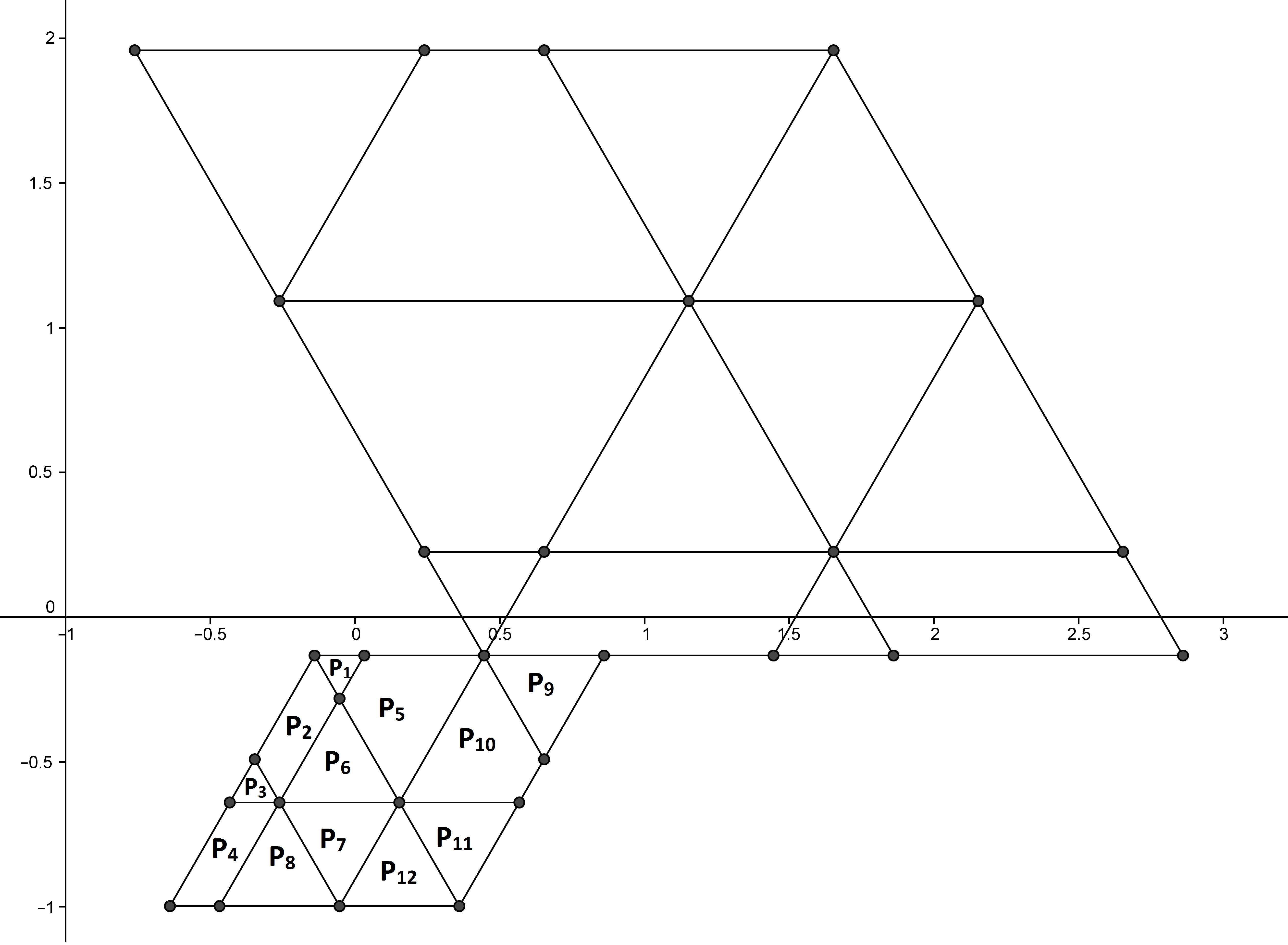
Let ζ=exp⁡(2​π​i/3)\zeta=\exp(2\pi i/3) and β=1+2\beta=1+\sqrt{2}. Set η1=1\eta_{1}=1 and η2=ζ2\eta_{2}=\zeta^{2} and (β​ζ−1)​ξ=3−β(\beta\zeta-1)\xi=3-\beta. From r⁡(ℒ)=1/3r(\mathcal{L})=1/\sqrt{3}, w⁡(𝒳)=3/2w(\mathcal{X})=\sqrt{3}/2 we have β>B2=7/3\beta>B_{2}=7/3 and there is a unique ACIM equivalent to Lebesgue measure by Theorem 1.1. We consider the symbolic dynamical system associated to the map TT. The set 𝒜\mathcal{A} is given by

{a=−1−ζ2,b=−ζ2,c=1−ζ2,d=2−ζ2,e=−2−2ζ2,f=−1−2ζ2,\displaystyle\bigl\{a=-1-\zeta^{2},b=-\zeta^{2},c=1-\zeta^{2},d=2-\zeta^{2},e=-2-2\zeta^{2},f=-1-2\zeta^{2},
g=−2ζ2,h=1−2ζ2,j=−2−3ζ2,k=−1−3ζ2,l=−3ζ2}.\displaystyle g=-2\zeta^{2},h=1-2\zeta^{2},j=-2-3\zeta^{2},k=-1-3\zeta^{2},l=-3\zeta^{2}\bigr\}.
Refer to caption
Figure 13. 𝒳\mathcal{X} and β​ζ​𝒳\beta\zeta\mathcal{X}

In Figure 13, we see that the discontinuity lines are finite and partition the fundamental domain 𝒳\mathcal{X} into disjoint components PnP_{n}, n=1,…,12n=1,\ldots,12. We also see in the figure the expanded fundamental region β​ζ​𝒳\beta\zeta\mathcal{X}.

It is easy to confirm that the image of PnP_{n} under TT is given by Table 1. From this table, we construct the sofic graph (see Figure 14) as described in §3.

Table 1.
nn T⁡(Pn)T(P_{n}) δ\delta
1 P7P_{7} bb
2 P11∪P12P_{11}\cup P_{12} bb
P4∪P7∪P8P_{4}\cup P_{7}\cup P_{8} cc
3 P12P_{12} cc
4 P11P_{11} cc
P4∪P7∪P8∪P12P_{4}\cup P_{7}\cup P_{8}\cup P_{12} dd
5 P9P_{9} aa
P1∪P2∪P5∪P6P_{1}\cup P_{2}\cup P_{5}\cup P_{6} bb
P7∪P11∪P12P_{7}\cup P_{11}\cup P_{12} ff
P4∪P7∪P8P_{4}\cup P_{7}\cup P_{8} gg
6 P9∪P10P_{9}\cup P_{10} bb
P2∪P3∪P6P_{2}\cup P_{3}\cup P_{6} cc
P12P_{12} gg
7 P1∪P5P_{1}\cup P_{5} cc
P11P_{11} gg
P4∪P7∪P8P_{4}\cup P_{7}\cup P_{8} hh
nn T⁡(Pn)T(P_{n}) δ\delta
8 P9∪P10P_{9}\cup P_{10} cc
P2∪P3∪P6P_{2}\cup P_{3}\cup P_{6} dd
P12P_{12} hh
9 P9P_{9} ee
P1∪P2P_{1}\cup P_{2} ff
P7∪P11∪P12P_{7}\cup P_{11}\cup P_{12} jj
P4P_{4} kk
10 P5∪P6∪P9∪P10P_{5}\cup P_{6}\cup P_{9}\cup P_{10} ff
P2∪P3∪P6P_{2}\cup P_{3}\cup P_{6} gg
P7∪P8∪P12P_{7}\cup P_{8}\cup P_{12} kk
11 P1∪P5P_{1}\cup P_{5} gg
P11P_{11} kk
P4∪P7∪P8P_{4}\cup P_{7}\cup P_{8} ll
12 P9∪P10P_{9}\cup P_{10} gg
P2∪P3∪P6P_{2}\cup P_{3}\cup P_{6} hh
P12P_{12} ll
P1P_{1}P2P_{2}P3P_{3}P4P_{4}P5P_{5}P6P_{6}P7P_{7}P8P_{8}P9P_{9}P10P_{10}P11P_{11}P12P_{12}
Figure 14. Sofic graph for 33-fold rotation
Example 6.3.

This example is a kind of a square root system of the negative beta expansion introduced by Ito-Sadahiro [7]. Let ζ=i\zeta=i and set η1=1\eta_{1}=1, η2=β​i\eta_{2}=\beta i and ξ=−1−β​i\xi=-1-\beta i. We have

T⁡(x+y​i)=−β​y−⌊−β​y+1⌋+β​x​i.T\left(x+yi\right)=-\beta y-\left\lfloor-\beta y+1\right\rfloor+\beta xi.

By taking its square, we can separate the variables:

T2​(x+y​i)=−β2​x−⌊−β2​x+1⌋+(−β2​y−β⁡⌊−β​y+1⌋)​i.T^{2}\left(x+yi\right)=-\beta^{2}x-\left\lfloor-\beta^{2}x+1\right\rfloor+\left(-\beta^{2}y-\beta\left\lfloor-\beta y+1\right\rfloor\right)i.

Thus we can study this map Gaussian coordinate-wise by defining

f⁡(x)=−β2​x−⌊−β2​x+1⌋,f(x)=-\beta^{2}x-\left\lfloor-\beta^{2}x+1\right\rfloor,

a 11-dimensional piecewise expansive map from [−1,0)\left[-1,0\right) to itself and

g⁡(y)=−β2​y−β⁡⌊−β​y+1⌋g(y)=-\beta^{2}y-\beta\left\lfloor-\beta y+1\right\rfloor

defined on [−β,0)\left[-\beta,0\right). We easily see that ff and gg give isomorphic systems through the relation g⁡(β​x)=β​f​(x)g(\beta x)=\beta f(x). Liao-Steiner [16] showed that the unique ACIM of ff is equivalent to the 11-dimensional Lebesgue measure if and only if β2≥(1+5)/2\beta^{2}\geq(1+\sqrt{5})/2. Thus the ACIM of TT is equivalent to the 22-dimensional Lebesgue measure if and only if β≥(1+5)/2\beta\geq\sqrt{(1+\sqrt{5})/2}. In view of the shape of ff, one see that if β2\beta^{2} is a Pisot number, then the system (𝒳,T)(\mathcal{X},T) is sofic (cf. Theorem 3.3 in [10]). This give examples of sofic rotational beta expansion beyond the scope of Theorem 1.5. One can also show that when β\beta is the Salem number whose minimum polynomial is x4−x3−x2−x+1x^{4}-x^{3}-x^{2}-x+1, the system becomes sofic.

This example is essentially 11-dimensional. We do not yet succeed in giving a ‘genuine’ 22-dimensional sofic rotational beta expansion beyond Theorem 1.5.

Example 6.4.

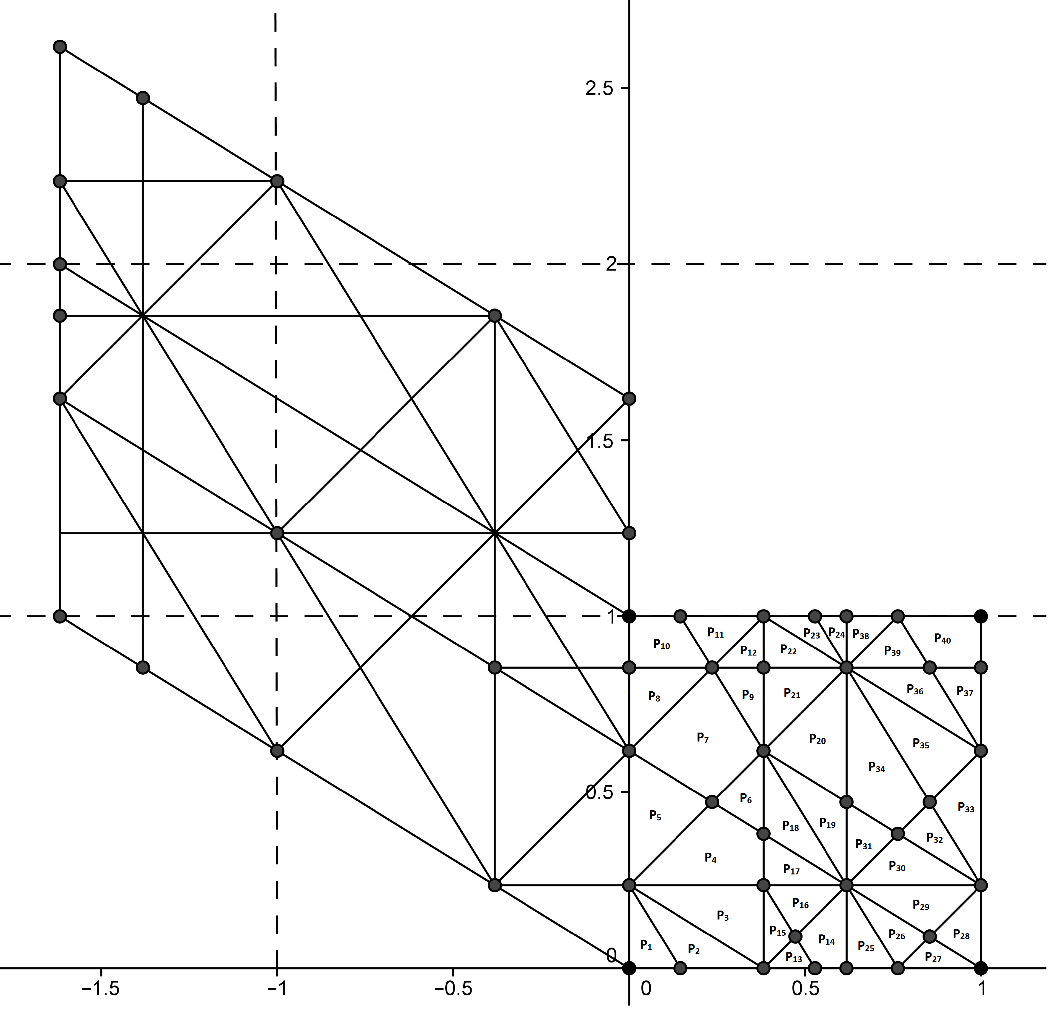
Let ξ=0\xi=0, η1=1\eta_{1}=1 and η2=ζ=exp⁡(2​π​i/5)\eta_{2}=\zeta=\exp(2\pi i/5). Let β=1+52\beta=\frac{1+\sqrt{5}}{2}. We describe the symbolic dynamical system associated to given rotation beta transformation through its sofic graph. Here, we use the map UU instead of TT. The alphabet 𝒜=Δ+(b1b2)=Δ\mathcal{A}=\Delta+\left(\begin{matrix}b_{1}\\ b_{2}\\ \end{matrix}\right)=\Delta is given by

{a=(−20),b=(−10),c=(−21),d=(−11),e=(−22),f=(−12)}.\left\{a=\left(\begin{matrix}-2\\ 0\\ \end{matrix}\right),b=\left(\begin{matrix}-1\\ 0\\ \end{matrix}\right),c=\left(\begin{matrix}-2\\ 1\\ \end{matrix}\right),d=\left(\begin{matrix}-1\\ 1\\ \end{matrix}\right),e=\left(\begin{matrix}-2\\ 2\\ \end{matrix}\right),f=\left(\begin{matrix}-1\\ 2\\ \end{matrix}\right)\right\}.

The partition of the fundamental region [0,1)2[0,1)^{2} is given in Figure 15. The sofic graph is described in Table 2. Since the incidence matrix of this graph is primitive, we can determine the ACIM whose density is positive and constant on each partition. Therefore the ACIM is equivalent to the Lebesgue measure, although we can not apply Theorem 1.1 for β<2\beta<2.

Table 2.
nn U⁡(Pn)U(P_{n}) δ\delta
1 P28∪P29P_{28}\cup P_{29} bb
2 P30∪P32∪P33P_{30}\cup P_{32}\cup P_{33} bb
3 P31∪P34∪P35P_{31}\cup P_{34}\cup P_{35} bb
4 P9∪P12∪P19∪P20∪P21∪P22P_{9}\cup P_{12}\cup P_{19}\cup P_{20}\cup P_{21}\cup P_{22} bb
5 P6∪P7∪P18P_{6}\cup P_{7}\cup P_{18} bb
6 P11P_{11} bb
P2P_{2} dd
7 P37∪P40P_{37}\cup P_{40} aa
P8∪P10P_{8}\cup P_{10} bb
P26∪P27∪P28∪P29P_{26}\cup P_{27}\cup P_{28}\cup P_{29} cc
P1P_{1} dd
8 P36∪P38∪P39P_{36}\cup P_{38}\cup P_{39} aa
P25P_{25} cc
9 P30∪P31P_{30}\cup P_{31} cc
10 P23∪P24P_{23}\cup P_{24} aa
P13∪P14∪P15∪P16P_{13}\cup P_{14}\cup P_{15}\cup P_{16} cc
11 P17∪P18P_{17}\cup P_{18} cc
12 P19P_{19} cc
13 P37P_{37} bb
14 P40P_{40} bb
P26∪P27P_{26}\cup P_{27} dd
15 P36P_{36} bb
16 P38∪P39P_{38}\cup P_{39} bb
P25P_{25} dd
17 P23∪P24P_{23}\cup P_{24} bb
P13∪P14P_{13}\cup P_{14} dd
18 P3∪P15∪P16P_{3}\cup P_{15}\cup P_{16} dd
19 P4∪P17P_{4}\cup P_{17} dd
20 P33∪P35P_{33}\cup P_{35} cc
P5P_{5} dd
nn U⁡(Pn)U(P_{n}) δ\delta
21 P32∪P34P_{32}\cup P_{34} cc
22 P20P_{20} cc
23 P21P_{21} cc
24 P22P_{22} cc
25 P28∪P29P_{28}\cup P_{29} dd
26 P30∪P32P_{30}\cup P_{32} dd
27 P33P_{33} dd
28 P35P_{35} dd
29 P31∪P34P_{31}\cup P_{34} dd
30 P19∪P20P_{19}\cup P_{20} dd
31 P6∪P18P_{6}\cup P_{18} dd
32 P9∪P21P_{9}\cup P_{21} dd
33 P11∪P12∪P22P_{11}\cup P_{12}\cup P_{22} dd
P2P_{2} ff
34 P36∪P37P_{36}\cup P_{37} cc
P7∪P8P_{7}\cup P_{8} dd
35 P39∪P40P_{39}\cup P_{40} cc
P10P_{10} dd
P27∪P28P_{27}\cup P_{28} ee
P1P_{1} ff
36 P38P_{38} cc
P25∪P26∪P29P_{25}\cup P_{26}\cup P_{29} ee
37 P30∪P31P_{30}\cup P_{31} ee
38 P23P_{23} cc
P13∪P15P_{13}\cup P_{15} ee
39 P24P_{24} cc
P14∪P16P_{14}\cup P_{16} ee
40 P17∪P18∪P19P_{17}\cup P_{18}\cup P_{19} ee
Refer to caption
Figure 15. 5-fold sofic case
Example 6.5.

Let ξ=0\xi=0, η1=1\eta_{1}=1 and η2=ζ=exp⁡(2​π​i/7)\eta_{2}=\zeta=\exp(2\pi i/7). Let β=1+2​cos⁡(2​π/7)≈2.24698\beta=1+2\cos(2\pi/7)\approx 2.24698, a cubic Pisot number whose minimum polynomial is x3−2​x2−x+1x^{3}-2x^{2}-x+1. From r⁡(ℒ)=1/(2​cos⁡(π/7))r(\mathcal{L})=1/(2\cos(\pi/7)), w⁡(𝒳)=sin⁡(2​π/7)w(\mathcal{X})=\sin(2\pi/7) we have β>B1≈2.00272\beta>B_{1}\approx 2.00272 and there is a unique ACIM by Theorem 1.1, but β<B2≈2.41964\beta<B_{2}\approx 2.41964. From Theorem 1.5, we know that the corresponding dynamical system is sofic. Figure 16 shows the sofic dissection of 𝒳\mathcal{X} by 224 discontinuity segments. The number of states of the sofic graph is 3292 (!), computed by Euler’s formula. It is possible to show that the corresponding incidence matrix of the sofic graph is primitive, and consequently the ACIM is equivalent to the Lebesgue measure.

Refer to caption
Figure 16. Sofic 7-fold rotation

References

  • [1] S. Akiyama, A family of non-sofic beta expansions, Ergodic Theory and Dynamical Systems, FirstView Article pp 1 -12, Published online: Aug 2014, doi: 10.1017/etds.2014.60
  • [2] S. Akiyama, H. Brunotte, A. Pethő, and J. M. Thuswaldner, Generalized radix representations and dynamical systems II, Acta Arith. 121 (2006), 21–61.
  • [3] J. Buzzi and G. Keller, Zeta functions and transfer operators for multidimensional piecewise affine and expanding maps, Ergodic Theory Dynam. Systems 21 (2001), no. 3, 689–716.
  • [4] J. H. Conway and N. J. A. Sloane, Sphere packings, lattices and groups, Grundlehren der Mathematischen Wissenschaften, vol. 290.
  • [5] W. J. Gilbert, Radix representations of quadratic fields, J. Math. Anal. Appl. 83 (1981), 264–274.
  • [6] P. Góra and A. Boyarsky, Absolutely continuous invariant measures for piecewise expanding C2C^{2} transformation in 𝐑N{\bf R}^{N}, Israel J. Math. 67 (1989), no. 3, 272–286.
  • [7] Sh. Ito and T. Sadahiro, Beta-expansions with negative bases, Integers 9 (2009), A22, 239–259.
  • [8] Sh. Ito and Y. Takahashi, Markov subshifts and realization of β\beta-expansions, J. Math. Soc. Japan 26 (1974), no. 1, 33–55.
  • [9] C. Kalle, Isomorphisms between positive and negative β\beta-transformations, Ergodic Theory Dynam. Systems 34 (2014), no. 1, 153–170.
  • [10] C. Kalle and W. Steiner, Beta-expansions, natural extensions and multiple tilings associated with Pisot units, Trans. Amer. Math. Soc. 364 (2012), no. 5, 2281–2318.
  • [11] I. Kátai and B. Kovács, Canonical number systems in imaginary quadratic fields, Acta Math. Acad. Sci. Hungar. 37 (1981), 159–164.
  • [12] G. Keller, Ergodicité et mesures invariantes pour les transformations dilatantes par morceaux d’une région bornée du plan, C. R. Acad. Sci. Paris Sér. A-B 289 (1979), no. 12, A625–A627.
  • [13] by same author, Generalized bounded variation and applications to piecewise monotonic transformations, Z. Wahrsch. Verw. Gebiete 69 (1985), no. 3, 461–478.
  • [14] V. Komornik and P. Loreti, Expansions in complex bases, Canad. Math. Bull. 50 (2007), no. 3, 399–408.
  • [15] T.Y. Li and J. A. Yorke, Ergodic transformations from an interval into itself, Trans. Amer. Math. Soc. 235 (1978), 183–192.
  • [16] L. Liao and W. Steiner, Dynamical properties of the negative beta-transformation, Ergodic Theory Dynam. Systems 32 (2012), no. 5, 1673–1690.
  • [17] D. Lind and B. Marcus, An introduction to symbolic dynamics and coding, Cambridge University Press, Cambridge, 1995.
  • [18] W. Parry, On the β\beta-expansions of real numbers, Acta Math. Acad. Sci. Hungar. 11 (1960), 401–416.
  • [19] A. Rényi, Representations for real numbers and their ergodic properties, Acta Math. Acad. Sci. Hungar. 8 (1957), 477–493.
  • [20] B. Saussol, Absolutely continuous invariant measures for multidimensional expanding maps, Israel J. Math. 116 (2000), 223–248.
  • [21] M. Tsujii, Absolutely continuous invariant measures for piecewise real-analytic expanding maps on the plane, Comm. Math. Phys. 208 (2000), no. 3, 605–622.
  • [22] by same author, Absolutely continuous invariant measures for expanding piecewise linear maps, Invent. Math. 143 (2001), no. 2, 349–373.