Effect of charging on CdSe/CdS dot-in-rods single photon emission.
Abstract
The photon statistics of CdSe/CdS dot-in-rods nanocrystals is studied with a method involving post-selection of the photon detection events based on the photoluminescence count rate. We show that flickering between two states needs to be taken into account to interpret the single-photon emission properties. With post-selection we are able to identify two emitting states: the exciton and the charged exciton (trion), characterized by different lifetimes and different second order correlation functions. Measurements of the second order autocorrelation function at zero delay with post-selection shows a degradation of the single photon emission for CdSe/CdS dot-in-rods in a charged state that we explain by deriving the neutral and charged biexciton quantum yields.
pacs
8.67.Bf,42.50.Ar,78.55.Cr,79.20.FvI Introduction
Wet-chemically synthesized colloidal core/shell nanocrystals (NCs) have been shown to emit non-classical light at room temperature [1, 2, 3, 4] making them suitable for applications in the field of quantum optics. Among colloidal NCs, CdSe/CdS dot-in-rods (DRs) made up by a spherical core of CdSe surrounded by a rod-like shell of CdS[5] have interesting features as single photon emitters such as a high degree of linear polarization [6, 7, 8, 9, 10] and a strongly reduced emission intermittency (non-blinking emission) when synthesized with thick CdS shells [11]. The emission of these nanostuctures at room temperature comes from the relaxation of various states, namely the exciton, the charged exciton and the neutral and charged multiexcitons. This diversity of emission states makes the interpretation of photon statistics quite difficult. Different emission states are characterized by different photons statistics and a study of the whole photons set detected from a given nanocrystal only gives an average behavior which can differ from particle to particle in the same batch. The photon statistics study is also a way to retrieve information about the charges relaxation processes such as Auger non-radiative recombination [12, 13]. A deeper understanding of the photon statistics is therefore a requirement for the comprehension of the emission processes of such nanoemitters.
Auger process in colloidal nanocrystals is at the origin of single-photon emission [14, 4] and it is suggested to be involved in blinking process [15, 16, 11] in such structures. Auger effect is a three-charge process in which the recombination energy of an electron-hole pair is transferred to an additional charge. Fast Auger non-radiative recombinations of multiexciton states leads to a nonradiative cascade decay of the excited states explaining the single-photon emission, hence multiphoton emission is quenched. However, if an extra charge is present in the crystal, Auger non-radiative recombination with the extra charge leads to the quenching of the exciton emission and blinking. Recent works [17, 18, 19] on CdSe/CdS spherical dots have demonstrated the importance of the geometry and the charge delocalization in influencing the Auger recombination rates. By growing NCs with a thicker shell around the core, it has been shown that charged nanocrystals still emit light owing to a less efficient Auger transfer. A negatively charged nanocrystal in a trion state has been shown to have an emission efficiency lower [17, 18] than or equal [19] to the pure exciton state. Several works have been devoted to the study of photon statistics as a method to assess the efficiency of the Auger processes and their consequence on multiexciton recombinations and blinking[12, 13]. Nair et al. [20] have demonstrated that one can deduce the biexciton quantum yield from the intensity autocorrelation function at zero delay, , for NCs pumped at low fluences.
In the present paper, we study the emission properties of DRs in terms of photon statistics. We show that a degradation of the single photon emission is associated with a charged nanocrystal by post-selecting photons based on their associated count rates after binning the signal [17]. This method allows to quantify separately the photon statistics associated with the two states of charge of such nanostructures. We explain the difference of photon statistics between a neutral and charged DR by evaluating the neutral and charged exciton and biexciton quantum yields. First, we present the emission characteristics of our DRs in terms of a flickering between a bright and a grey state. Thanks to post-selection on the photon detection events, we can reconstruct the autocorrelation function of the bright and grey state separately. Comparing two DRs from the same batch, which display different exciton lifetimes, we explain the differences observed for the photon statistics in terms of charge delocalization and flickering between the two states.
II Experimental set-up
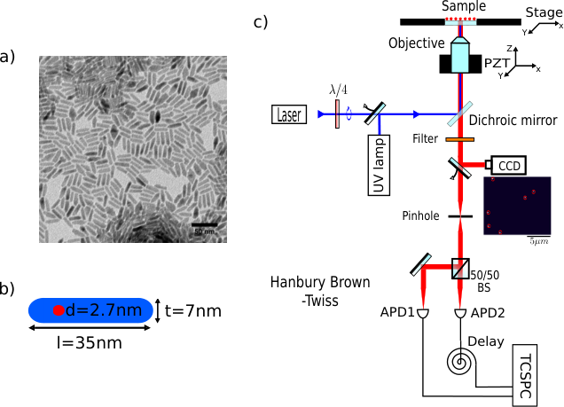
We used high quality CdSe/CdS core-shell DRs synthesized using the seeded growth approach proposed in reference[5, 11]. A transmission electron microscope (TEM) image of the investigated sample before dilution is presented in Fig.1a. The DRs are characterized by a shell length nm, a thickness nm and a core diameter nm as depicted in Fig.1b. A dilute solution is drop-casted on a microscope glass coverslip to produce a low density of single DRs ( to DRs per m2 area). Wide field luminescence microscopy can be realized using a UV lamp to excite a broad area of the sample. Imaging of the excited area on a high quantum efficiency CCD camera gives an overview of the sample as shown in Fig.1c with a zoom on a m2 area. A single DR can be subsequently chosen and excited using a picosecond-pulsed laser diode with a small excitation spot of m2. The picosecond-pulsed laser operates at a wavelength of nm to excite the highly absorptive shell [5], with a repetition rate of MHz such that the time between two laser pulses is typically greater than an absorption emission cycle duration. To obtain an excitation independent of DRs orientations on the substrate the laser light is circularly polarized. The photoluminescence (PL) is collected using a confocal microscope with a high numerical aperture oil immersion objective (, N.A.=). A high pass filter (cutoff nm) removes the remaining excitation light while leaving the DRs photoluminescence which is centered around nm. The DR photoluminescence is then spatially filtered through a pinhole (diameter m) and subsequently recorded using two single-photon avalanche photodiodes (APD) in a Hanbury-Brown and Twiss configuration as shown in Fig.1c. The signals from the photodiodes were recorded by a Time-Correlated Single Photon Counting (TCSPC) data acquisition card (PicoHarp300,Picoquant) enabling for each DR the recording of the PL lifetimes and the PL autocorrelation function.
III Flickering
The DRs investigated in this study are well described by a fast switching (flickering) between two states of emission: a bright state with a high emission efficiency and a grey state with a lower emission efficiency [17, 11]. The emission efficiency is assessed by the quantum yield (QY) which is given by the ratio between the radiative decay rate and the total decay rate due to radiative and non-radiative relaxations. Excitons in high quality CdSe structures have a QY close to unity [21, 22], while the trion state exhibits a QY ranging from to in this specific sample [11].
Representative emission properties from a single DR, namely DR1, are displayed in Fig.2. Fig.2a shows the photoluminescence (PL) intensity recorded during 15 seconds with a bin time of s, for a low excitation power corresponding to an average number of electron hole pairs excited by a single laser pulse of . A zoom on a ms time window is also shown. The switching between the two states is clear on the shorter time window of ms. The red part of the time trace above counts/ms corresponds to the bright state while the green part below counts/ms can be attributed to the grey state. In Fig.2b, the histogram of the PL intensity confirms the presence of two states. A fit of this histogram with two Poissonian distributions reproduces the intensity distribution properly, except in the intermediate region. In the following, the post-selected photons of a given state are chosen based on the intensity histogram. If a time bin has a number of photons such that it falls into a state intensity window, then the photons of this time bin are associated to this state. All subsequent data analysis for a given state, such as PL lifetime or autocorrelation function, are realized with the chosen photons from the intensity histogram.
For long timescales, Fig.2c shows the normalized second order autocorrelation functions (ACF), as given by Eq.(1) at the beginning of section IV. Long timescales here means that we present the function with a resolution and on timescales longer than the emitter lifetime and laser repetition rate. Therefore no antibunching and quantum properties of the emitter are revealed with this measurement but information on the flickering can be retrieved. From top to bottom respectively, the for the photons inside the grey state count rate range ( to counts/ms), the for the photons inside the bright state count rate range (above counts/ms) and finally the of all the recorded events displayed in Fig.2a are shown. When no count rate range is chosen (Fig.2c bottom), a super-Poissonian statistics with of is observed on timescales ranging from s to ms due to the flickering between the two states [23, 24]. For delays above ms the falls down to one, meaning that switching between the two states does not happen on these longer timescales owing to a reduced blinking for these thick shells DRs [11]. As flickering occurs even at microseconds timescales, it is always faster than any typical bin time used to build the intensity distribution. There is no perfectly appropriate bin time to fully discriminate the two states and binning the signal always leads to a mix of the two states. Therefore the transition between the two states is blurred and the system is not well described by a superposition of two Poissonian states in the transition region as seen in Fig.2b (blue line). In contrast, the functions in Fig.2c for the selected photons of the grey (top) and bright (middle) states have a value of one at every timescales displayed. This is a strong evidence that our post-selection of the photon detection events discriminates well between the photons of the two states as no additional bunching (super-Poissonian statistics) due to the flickering is present. The photons associated with the intensities between counts/ms and counts/ms inside the central region of the intensity histogram in Fig.2b cannot be attributed to a specific state and have therefore been discarded. They represent of the photon events recorded for this specific measurement, while the grey and bright state photons represent and of the recorded photons respectively.
We further confirm the analysis of the PL properties of our DRs in terms of switching between a bright and a grey state by studying the PL decay. In Fig.2d, while the full PL decay (blue diamonds) cannot be fitted with a single exponential, post-selecting only the photons recorded in the red intensity window in Fig.2d (red squares), the PL decay is nearly mono-exponential with a decay constant of ns. The PL of the photons in the green intensity window (green circles) in Fig.2c is found to decay exponentially with a time constant ns. These two time constants are attributed to the neutral and the negatively charged exciton (X and ) as demonstrated in the literature[18]. They correspond to the bright and grey states respectively. These results allow to evaluate the emission quantum yields. The exciton quantum yield is defined as: with , the radiative and non-radiative decay rates respectively and the measured exciton lifetime. Assuming [21, 22, 11], the radiative decay rate is simply the inverse of the measured exciton lifetime. Using statistical scaling [25, 19], the trion radiative decay rate can be shown to be twice as fast as the neutral exciton because of the creation of a new radiative relaxation path by the extra charge (an electron in this case). The trion QY is therefore given by: , which gives , using the data of Fig.2d. The mean intensities in Fig.2.b where counts/ms is equal to of the mean exciton intensity ( counts/ms) confirms the statistical scaling approach and the consistence of our model. The lower QY of the trion comes from the fact that the extra electron opens not only a new radiative relaxation channel but also a non-radiative channel. This non-radiative channel is due to an Auger process[25], which is the relaxation of the electron hole pair to the extra electron. The non-radiative decay rate for a negatively charged DR is therefore equal to the Auger relaxation rate: .
We have shown that the emission of our DRs is well described by a fast switching between a bright and a grey state. Post-selection of the photon detection events based on the intensity count rates for a given bin time can successfully discriminate between the photons of each state as attested by the functions in Fig.2c and by the pure exponential decay of the two states. In the following, using post-selection of the photon events, we show that we can retrieve the biexciton and charged biexciton QYs from the autocorrelation function at zero delay and explain the differences in the photon statistics obtained with different DRs.
IV Flickering and Biexciton emission
The normalized intensity autocorrelation function is obtained from the numbers of counts and measured in the two channels of the Hanbury-Brown and Twiss set-up as a function of the delay between the two channels. It is given by:
| (1) |
In ref.[20], a general equation is derived to express the autocorrelation function at zero delay for a single nanocrystal depending on the probability to excite a given number of electron-hole pairs and the multiexciton quantum yields of the different excited states. The probabilities that at least excitons are created inside the nanocrystal for an excitation energy well above the exciton line, in the continuum of the shell states, a condition typically realized in our experiment, is:
| (2) |
where is the average number of excitations inside the nanocrystal. This is a sum of Poissonian distributions which only depends on the excitation power since the excitation is far above the bandgap. For a single nanocrystal weakly pumped, higher order multiexcitons are not excited. In this case, the probability to emit two photons through a radiative decay of the biexciton and exciton is , the product of the quantum yields of the two states weighted by the probability to excite at least two electron hole pairs, while the probability to emit one photon is . As shown in appendix A, reduces to twice the probability to emit two photons over the probability to emit one photon squared:
| (3) |
In a very weak pumping regime such that , Eq.(3) simplifies to:
| (4) |
as . This formula has been used in [20, 12, 13] to derive the biexciton quantum yield from an ACF measurement. This implies that an emitter having a non zero biexciton quantum yield will not show complete antibunching even at very low pumping regime.
In the following we will consider an excitation power such that . The weighting term in Eq.(3) is in this case. This excitation power has been chosen such that the grey state generated by photoionization could be clearly observed. This is typically realized when the probability to excite at least two electron-hole pairs is high enough, here . In this case, ionization events through Auger processes are sufficiently frequent to observe the grey state in the PL intensity distribution, which is not the case at lower excitation. At this excitation power , this ensures that higher excited states such as a doubly charged exciton for example are very unlikely, validating our two states model for the emission. Fig.3 presents the different relaxation possibilities for such an excitation, . First possibility, the DR is in a neutral state. Starting from two excitons in the structure, the DR will emit one photon with probability after Auger non-radiative relaxation of the biexciton with rate or depending to which charge the energy is given to (a hole or an electron as depicted on Fig.3a). Or it will emit two photons with probability if no Auger relaxation takes place (Fig.3b). Second possibility, the DR is in a charged state. It will either emit one (Fig.3d) or two photons (Fig.3e) with probabilities and respectively, with the charged biexciton QY. Non radiative Auger transfer to the extra electron with rate can also quench the emission and no photon will be emitted (Fig.3c).
Quantifying the change in QYs between neutral and charged DRs using post-selection of the photon detection events will allow us to understand the change in photon statistics due to charging. The overall photon statistics of a DR resulting in an interplay between the neutral and charged photon statistics is explained below. Differences of photon statistics between DRs is also presented and explained in sectionV.
In the following, Eq.(3) will be therefore applied to the post-selected photons of each state separately, thus providing information on the biexciton and charged biexciton QYs through the exciton and trion autocorrelation function:
| (5) |
To realize this analysis, the post-selected photons are chosen inside intensity windows such that the number of photons is maximized to have the largest statistics and the mix between the two states is minimized. This last point is assessed using the values on several decades of delays between photons as in Fig.2c. A equal to one for the photons from a given intensity window for all photon delays is an evidence that we are selecting photons from only one state of emission.
Fig.4 shows the ACF for DR1 whose emission characteristics were presented in section III. If computed with a time resolution shorter than the emitter lifetime, the ACF consists in a series of peaks with a time interval corresponding to laser repetition rate. In this case, the quantum nature of the emission is evidenced by the antibunching, the peak at zero delay being smaller than the other peaks. The ACF has been normalized such that to each peak height corresponds the value found at longer delays in Fig.2c. The value can thus be easily found by looking at the height of the peak at zero delay. DR1 gives for the grey state, larger than for the the bright state by a factor of . A degradation of the single photon emission properties is therefore associated with a DR in a charged state. We can also observe that for all the detection events , it is close to the bright state photon statistics as . The grey state photon proportion for this measurement is low: , the bright state photons representing of the measured events and the discarded photons as already mentioned in section III. Hence, the bright state photon statistics is very close to the overall photon statistics.
As can be seen from Eq.(5), the degradation of the single photon emission with charging is related to the increase of the ratio between the biexciton and exciton QY. A higher value is therefore not necessarily due to an increase of the two photon emission but can also be the result of a decrease in the single photon emission. In order to go further, the various QYs involved in Eq.(5) have to be quantified to see the effect of the charging on the single photon and two photon emission.
In quasi-type II structures such as CdSe/CdS DRs [11], the conduction band offset between the two materials being fairly weak the electron is not well confined inside the CdSe core but instead delocalized on the whole structure. Conversely, the holes are well confined into the CdSe core due to a higher offset between the valence bands of the two materials. The Auger rates to a hole and to an electron can therefore be different as they scale with the confinement volume [26]. In the following section, we study the consequences of different Auger rates corresponding to energy transfer to positive (hole) and negative (electron) charges on the photon statistics. To do so we present measurements on another DR (namely DR2) from the same sample as DR1 that presents a much shorter exciton lifetime ns than DR1 ( ns). As the value of the exciton lifetime is directly linked to the overlap between the electron and hole wavefunctions, it is an indication of the electron delocalization. We expect different photon statistics for these two DRs.
V Charge delocalization and biexciton emission
We now proceed to a comparison between DR1 characterized by a long lifetime ( ns) and therefore a highly delocalized electron and DR2 characterized by a shorter lifetime ( ns) and consequently a more localized electron. Fig.5 shows the histogram of PL emission, the PL decay and photon statistics of DR2. First, it appears that this DR is characterized by a lower grey state QY, compared to DR1 (). The trion state is less emissive in this case because of a higher efficiency of the Auger relaxation process to the extra electron, the only non-radiative decay channel. A higher efficiency of the Auger process is explained in this case by the more confined electron compared to DR1 as the Auger effect scales with the volume occupied by the charge [26]. The of all the photon detection events (Fig.5c bottom) is characterized by a bunching on the same timescales as DR1, from microseconds delays to tenth of milliseconds. The bunching value of is higher owing to a higher discrepancy of QYs between the two states together with an increased grey state photon proportion () compared to DR1 (). The post-selection of photon events with count rates below counts/ms and above counts/ms for the grey and bright states respectively in Fig.5a allows us to discriminate the photons of each state. The corresponding to the bright state (Fig.5c middle) has a value of 1 at all delay timescales. A limited bunching is still visible for the grey state with a value of at short delays. Taking a smaller intensity window does not change this value. A fast flickering dynamic between the two states for DR2 that cannot be resolved correctly with the short binning time of s very likely explains an imperfect photon sorting and consequently this small remaining bunching. For this specific DR we discard of the registered photons.
The bright state photon statistics for DR2 is similar to DR1,with for DR2 versus for DR1. The two neutral DRs have comparable single (excitonic) and two photon (biexcitonic) emission statistics. The grey state photon statistics is nevertheless different. The degradation of the single photon emission is more important for DR2 with versus for DR1. For DR2 the value corresponding to all the photons is equal to , it is almost twice the value found for DR1. This difference can be explained by the proportion of photons of each state in the overall measurement. The grey state photon proportion being three times larger for DR2 than for DR1, is therefore increasing towards the charged exciton photon statistics. The at zero delay of the entire photon events detection reflects therefore the interplay between the two states characterized by different photon statistics.
In order to go further in this comparison, we calculate the quantum yields of the various states. The quantum yield of the trion is obtained from the ratio between the grey and bright state lifetimes assuming [21, 22]. These results are given in the third column of Table 1 for the two considered DRs. The quantum yield of the trion varies from (DR1) to (DR2) of the exciton quantum yield. Then and are calculated using Eq.(5), with the values of and from diagrams in Fig.4 for DR1 and Fig.5d for DR2 and with corresponding to . Table 1 gives the quantum yield of the neutral biexciton and of the charged biexciton . The values of the neutral biexciton quantum yields are similar for the two DRs and close to , corresponding to similar low values of obtained for the neutral state. The values for the charged biexciton quantum yields ( for DR2 and for DR1) are found to be from % to almost % of the neutral biexciton quantum yield. This means that charging affects the biexciton quantum yield less than the exciton quantum yield. In fact, as mentioned above, the QY of the charged exciton (trion) is much smaller than the one of the exciton, yielding an increase of compared to . Thus, remarkably, the increase of when a DR is charged is not due to a higher probability of two photon emission compared to a neutral DR but to the fact that the two photon emission probability decreases slower than the single photon emission probability squared.
Finally, the evolution of the various QYs for these two DRs allows us to gain information on the relaxation processes in the DRs. As mentioned above, the dominant non radiative relaxation process is the Auger effect. The Auger relaxation rate of an electron hole pair to a neighboring electron can be derived from the negative trion state QY [19]:
| (6) |
In the case of a biexciton, the energy of an electron-hole pair can be transferred to a negative or a positive charge (electron or hole) by an Auger process as depicted in Fig.3a, c and d. Assuming again that the non radiative decay channels are due only to the Auger effect the biexciton QY can be written as [19]:
| (7) |
This formula allows to deduce the Auger relaxation rate to a positive charge from the quantum yield of the biexciton.
For DR1, is found to be ns while the Auger relaxation to positive charges ns is almost four times faster. The long Auger relaxation lifetime for electrons can be explained by a highly delocalized electron inside the shell as expected from the long exciton lifetime ns. Auger relaxation to an electron is less efficient than to a hole because of electron delocalization in quasi type-II heterostructure like CdSe/CdS DRs [27]. In this case, positive charges constitute a preferred decay channel and the extra negative charge does not increase the number of non radiative relaxation paths as it is an inefficient relaxation solution. The biexciton mainly relaxes giving its energy to a well confined hole whether the DR is charged or not, thus in Fig.3 the scenari c and d are similar to the scenario a. This explains that for DR1 the negatively charged biexciton QY is the same as the neutral biexciton QY.
In contrast, for DR2 characterized by a shorter exciton lifetime of ns and consequently a less delocalized electron compared to DR1, using the same calculation, ns and ns have similar values. It implies in this case a decrease of the charged biexciton QY compared to the neutral biexciton QY. No decay channel for the biexciton is favored in this case, so when a DR is charged, the extra negative charge offers an additional non radiative decay channel, as can be seen on Fig.3c and d, which decreases the charged biexciton QY compared to the neutral biexciton QY. These different behaviors probably come from a slightly different structure of DR2 as compared to DR1, implying a different localization of the electrons and the holes in the two DRs as expected from the different exciton lifetimes. Our measurements thus give access to a full characterization and interpretation of the physical processes taking place in the DRs including photon emission, and Auger effects to positive and negative charges.
| (ns) | (ns) | (ns) | |||||
|---|---|---|---|---|---|---|---|
| DR1 | 65 | 100% | 36% | 10.6% | 10.1% | 18.3 | 4.9 |
| DR2 | 28 | 100% | 18% | 9.7% | 6.2% | 3.1 | 2.9 |
VI Conclusion
In conclusion we have shown that CdSe/CdS DRs emission was characterized by a fast switching between a bright and a grey state of the emission. Thanks to a post-selection of the emitted photons we could study independently the lifetimes and the intensity autocorrelation function of the bright and grey states. From this method we deduced the quantum yields of the charged exciton, of the biexciton and of the charged biexciton. In particular we have been able to explain the degradation of the second order autocorrelation function in charged DRs by the decrease of the single photon emission probability in the charged exciton rather than by an increase of the two-photon emission probability. By comparing two DRs from the same sample displaying different excitons lifetimes and consequently different charges localizations, the effects of the interplay between photon emission and Auger recombinations were illustrated. We were able to explain the differences between the overall photon statistics of these two DRs by quantifying the bright and grey state photons proportions and statistics. With this analysis we have thus obtained a fully quantitative model of single photon and two-photon emission of CdSe/CdS dot-in-rods with two states of emission.
Acknowledgements.
The authors gratefully thank Jean-Pierre Hermier for fruitful discussions. Financial support from the French research council ANR, under the project SENOQI, CNANO Sophopol and projet ITN-Clermont4Appendix A Derivation of Eq.(3).
It has been demonstrated in ref.[20] that the autocorrelation function at zero delay can be expressed as a function of the quantum yield of the different multiexcitonic states and the Poissonian probability, assuming the independence of the different multiexcitonic fluorescence processes:
| (8) |
where stands for a time average over the measurement acquisition time if any blinking occurs. Considering an emitter displaying antibunching, therefore having low multiexciton QY, the previous equation simplifies to:
| (9) |
which can be reduced to
| (10) |
for the typical excitation power considered in this paper . If no blinking occurs or if the photons are post-selected so as to separate the different states, then we retrieve Eq.(3):
| (11) |
References
- [1] A. I. P Michler et al., Nature 406, 968 (2000).
- [2] B. Lounis, H. Bechtel, D. Gerion, P. Alivisatos, and W. Moerner, Chemical Physics Letters 329, 399 (2000).
- [3] X. Brokmann, G. Messin, P. Desbiolles, E. Giacobino, M. Dahan, and J. Hermier, New Journal of Physics 6, 99 (2004a).
- [4] B. Fisher, J. M. Caruge, D. Zehnder, and M. Bawendi, Physical review letters 94, 087403 (2005).
- [5] L. Carbone, C. Nobile, M. De Giorgi, F. D. Sala, G. Morello, P. Pompa, M. Hytch, E. Snoeck, A. Fiore, I. R. Franchini, et al., Nano letters 7, 2942 (2007).
- [6] S. Vezzoli, S. Shojaii, S. Cialdi, D. Cipriani, F. Castelli, M. G. Paris, L. Carbone, P. Davide Cozzoli, E. Giacobino, and A. Bramati, Optics Communications 300, 215 (2013).
- [7] F. Pisanello, L. Martiradonna, G. Leménager, P. Spinicelli, A. Fiore, L. Manna, J.-P. Hermier, R. Cingolani, E. Giacobino, M. De Vittorio, et al., Applied Physics Letters 96, 033101 (2010a).
- [8] A. Sitt, A. Salant, G. Menagen, and U. Banin, Nano letters 11, 2054 (2011).
- [9] I. Hadar, G. B. Hitin, A. Sitt, A. Faust, and U. Banin, The Journal of Physical Chemistry Letters 4, 502 (2013).
- [10] F. Pisanello, L. Martiradonna, P. Spinicelli, A. Fiore, J. Hermier, L. Manna, R. Cingolani, E. Giacobino, M. De Vittorio, and A. Bramati, Superlattices and Microstructures 47, 165 (2010b).
- [11] F. Pisanello, G. Leménager, L. Martiradonna, L. Carbone, S. Vezzoli, P. Desfonds, P. D. Cozzoli, J.-P. Hermier, E. Giacobino, R. Cingolani, M. D. Vittorio, and A. Bramati, Adv. Mater. Weinheim 25, 1974 (2013).
- [12] Y.-S. Park, A. V. Malko, J. Vela, Y. Chen, Y. Ghosh, F. Garcia-Santamaria, J. A. Hollingsworth, V. I. Klimov, and H. Htoon, Physical review letters 106, 187401 (2011).
- [13] J. Zhao, O. Chen, D. B. Strasfeld, and M. G. Bawendi, Nano letters 12, 4477 (2012).
- [14] V. Klimov, A. Mikhailovsky, D. McBranch, C. Leatherdale, and M. Bawendi, Science 287, 1011 (2000).
- [15] M. Nirmal, B. Dabbousi, M. Bawendi, J. Macklin, J. Trautman, T. Harris, and L. Brus, Nature 383, 802 (1996).
- [16] A. L. Efros and M. Rosen, Physical Review Letters 78, 1110 (1997).
- [17] P. Spinicelli, S. Buil, X. Quelin, B. Mahler, B. Dubertret, and J.-P. Hermier, Physical review letters 102, 136801 (2009).
- [18] C. Galland, Y. Ghosh, A. Steinbrück, M. Sykora, J. A. Hollingsworth, V. I. Klimov, and H. Htoon, Nature 479, 203 (2011).
- [19] C. Galland, Y. Ghosh, A. Steinbrück, J. A. Hollingsworth, H. Htoon, and V. I. Klimov, Nature communications 3, 908 (2012).
- [20] G. Nair, J. Zhao, and M. G. Bawendi, Nano letters 11, 1136 (2011).
- [21] X. Brokmann, L. Coolen, M. Dahan, and J. Hermier, Physical review letters 93, 107403 (2004b).
- [22] B. R. Fisher, H.-J. Eisler, N. E. Stott, and M. G. Bawendi, The Journal of Physical Chemistry B 108, 143 (2004).
- [23] L. Fleury, J.-M. Segura, G. Zumofen, B. Hecht, and U. Wild, Physical review letters 84, 1148 (2000).
- [24] G. Messin, J. Hermier, E. Giacobino, P. Desbiolles, and M. Dahan, Optics Letters 26, 1891 (2001).
- [25] V. Klimov, J. McGuire, R. Schaller, and V. Rupasov, Physical Review B 77, 195324 (2008).
- [26] I. Robel, R. Gresback, U. Kortshagen, R. D. Schaller, and V. I. Klimov, Physical review letters 102, 177404 (2009).
- [27] A. Sitt, F. D. Sala, G. Menagen, and U. Banin, Nano letters 9, 3470 (2009).