A coefficient average approximation towards Gutzwiller wavefunction formalism
Abstract
Gutzwiller wavefunction is a physically well motivated trial wavefunction for describing correlated electron systems. In this work, a new approximation is introduced to facilitate evaluation of the expectation value of any operator within the Gutzwiller wavefunction formalism. The basic idea is to make use of a specially designed average over Gutzwiller wavefunction coefficients expanded in the many-body Fock space to approximate the ratio of expectation values between a Gutzwiller wavefunction and its underlying noninteracting wavefunction. To check with the standard Gutzwiller approximation (GA), we test its performance on single band systems and find quite interesting properties. On finite systems, we noticed that it gives superior performance than GA, while on infinite systems it asymptotically approaches GA. Analytic analysis together with numerical tests are provided to support this claimed asymptotical behavior. At the end, possible improvements on the approximation and its generalization towards multiband systems are illustrated and discussed.
Keywords:
strongly correlated electron system, Gutzwiller wavefunction, Gutzwiller approximation, single band Hubbard Model, multiband system, CCSD, GAMESSI Introduction
Correlation effects play an important role in electronic movements and physical properties of real materials[1]. Strong electron-electron interaction is believed to be key to fully understand many interesting phenomena, including high Tc superconductivity[2], heavy fermion behaviors[3], abnormal transport and optical properties[4], and more on strongly correlated materials. A versatile and convenient way to describe these systems has been posed as a big challenge to the solid state community in the past years. Part of the reasons are due to the strong Coulomb interaction preventing a controlled perturbative treatment which has been very successfully developed for weakly interacting systems. The conventional mean field treatment is most versatile in gaining insights to correlated electron systems on their possible new physics, competing phases and dynamical behaviors. But its conclusions are always in question whether the ignored residual electron correlation effects are still significant enough to overshadow the presumed mean-field behaviors[5][6]. To go beyond the mean field approximation, analytic tools were proposed based on infinite summation of Feynmann diagrams of chosen types, e.g., the Random Phase Approximation (RPA)[7], the spin fluctuation theory[8], and compact diagrammatic equations like the Fluctuation Exchange approximation (FLEX)[9] or the parquet formalism[10][11]. Although they offer alternative ways for people to use, their results might be biased by starting with a subjective choice of a subgroup of diagrams which are usually numerically convenient to deal with. On the side of computational physics, a number of tools exist including Exact Diagonalization (ED)[12], Quantum Monte Carlo simulation(QMC)[13], Dynamic Mean Field Theory (DMFT) and its cluster extensions[14][15][16], and renormalization group type methods[17][18][19]. These tools are computationally demanding and can suffer from serious finite size effects or other numerical complications.
On the other hand, the variational approach[20] has always been a very important category of methods in addressing a wide range of physical problems, thanks to its capability of conveniently incorporating clear physical insights into a well-designed trial wavefunction. A typical example is the ab initio local density approximation (LDA) which has become an indispensable tool in modern scientific and material research[21][22]. In strongly correlated systems, the variational approach can play an important role and has been shown to be very effective and enlightening in studying various correlation effects[23][24][25]. It avoids looking for a small quantity to validate a perturbative expansion of the problem, but instead, it focuses directly on most prominent physics out of correlation effects. A simple-minded way to take care of the local onsite correlation is to form a trial wavefunction with a local projection operator to control double occupancy. This brings up the famous Gutzwiller trial wavefunction to address local correlation effects[25]. Unfortunately, a direct evaluation of operator expectation values is not practical for a many-body wavefunction. How to form a new way to efficiently implement the Gutzwiller wavefunction formalism will be the focus of the current paper.
The typical model Hamiltonian to study correlation effects is the so-called single band Hubbard model[26] on a two-dimensional square lattice, expressed as
| (1) |
with denoting site indices and spins. Two energy scales, the hopping amplitude, between nearest neighboring sites and the onsite Hubbard interaction, exist and compete with each other. The correlation effect becomes dominant in case onsite energy is big as compared against hopping The ground state wavefunction is presumably well described by the Gutzwiller trial wavefunction (GWF) defined as
| (2) |
with the local Gutzwiller projector defined as
| (3) |
Here is defined as the local double occupancy operator and is the unknown Gutzwiller variational parameter, a positive number which controls the weight of electronic configurations containing double occupancy in the noninteracting wavefunction [27][25]. Although is defined purely locally, it might still capture some nonlocal physics through the 2nd order virtual hopping process in the strong correlation limit[28][29]. Thus Eq. 2 is a quite reasonable trial wavefunction to capture the essential physics of a correlated electron system.
However, introducing a physically sensible trial wavefunction is only the first step. Brute force evaluation of physical observables in a many-body system can be a real pain due to numerical difficulties and computer hardware capacity. Thus, the so-called Gutzwiller approximation (GA) was introduced to facilitate the evaluation[25][30][31][32]. There, the expectation value for an interacting system is assumed to be proportional to that of the noninteracting wavefunction through a site-decomposeable renormalization factor. Taking the hopping operator as an example, GA gives
| (4) |
for two distinct sites. Here, denote orbital indices and denotes spin. A succinct analytic expression for is available for the operator (or )[32]. Actually, we might come up with an educated guess that, given any local operator with the set of local spin-orbital states involved in , the corresponding is given as
| (5) |
with
| (6) |
Here and denotes the occupational probability at a local Fock state The summation in Eq. 5 traverses all local Fock states mutually related by the local operator One can go through the tedious yet well-established procedure to verify this relations for any operator[33]. The introduction of as a renormalization factor is physically very sensible. Strong correlation effects among electrons necessarily leave an impact on their motions, thus modifying their dynamical and transport behaviors as compared against a Fermi liquid system described by .
There have been roughly three different ways to reach GA. Metzner et al approached GA with mathematical rigor by applying Feymann diagrammatic expansion techinque to the Gutzwiller wavefunction[34][35]. The approach effectively cuts intersite communications in the infinite spatial dimension limit and leaves only intrasite correlations among local orbits. This brings up the main site-wise decomposibility feature of GA readily seen from the site-dependent renormalization factors illustrated in Eq. 4. This approach has been further carried out by Bunemann et. al. and Fabrizio et. al. to multiband systems and with a more generalized Gutzwiller projector[32][36] [37][38]. The second way of writing down GA is through physical intuition with a hand-waving argument. Gutzwiller originally formulated GA based on some assumptions[25] whose physics were rather obscure thus preventing it from being generalized to multiband systems. Ogawa’s counting argument formally pointed out that the physics underlying Gutzwiller’s GA is to assume that the expectation value of a product of number operators equals the product of expectation value of each number operator in the series[31]. The physics of GA is most transparent in Bunemann’s version of counting argument[32]. We regard it as a third approach towards GA due to its balance between clarity in physics and completeness in formulation. Bunemann made it clear that the projection of a noninteracting wavefunction onto a specific electronic configuration depends only on the number of electrons on each local orbital on the lattice, but not on how these electrons are distributed on the lattice. This implies two things. First, the combinatoric trick accompanying the assumption can be used to evaluate any inner product, which greatly simplifies the whole formalism and introduces an additional convenience of taking the thermodynamic limit to further simplify the expressions. Second, he pointed out that GA actually implies more than just one relation, but instead, infinitely many for different operators whose expectation values are to be evaluated. This leaves us a taste on how crude GA might work in reality.
Despite many achievements made by GA on qualitatively addressing the Mott physics in correlated electron systems, quantitatively however, it might introduce artifacts. For instance, GA predicts existence of a Brinkman-Rice metal-insulator transition at a critical onsite interaction comparable to the bandwidth in a single band system[39], while GWF formalism should always give metallic behavior unless [34]. These artifacts are of course closely related with the rough assumptions made in GA. The artificial Brinkman-Rice transition seems to imply excessive local correlations were introduced by GA. In addition, besides the unphysical infinite spatial dimension limit, the most questionable assumption in GA is that it calls for a presumably known connection between the Gutzwiller local orbital occupations and those of the noninteracting wavefunction, a requisite to facilitate the Feynman diagrammatic expansion to derive GA[32][33]. This might cause trouble in multiband systems where charge flow among orbitals might necessarily play a role due to correlation effects[40].
It would be useful if some of the concerns mentioned above could be addressed. However, within the existing GA formulation, this is not an easy task mainly because the formulation is mathematically prohibitively complicated to be further improved. Thus we need a new way to look into the renormalization factors of operators, central quantity of GA to bridge between the Gutzwiller and the noninteracting wavefunction. We come up with a very simple way to design the renormalization factors which gives the standard GA in the thermodynamic limit, and which also has the potential to be improved systematically. We might thus call it a fourth way to reach GA.
II Method
Let’s introduce some notations first to facilitate the up-coming discussion. Given a number of local spin-orbital states, the local Fock space is set up and denoted as Specifically, in the single band case, we denote the spin-orbital states as with the orbital index, and note Here denotes an empty state and denotes a singly occupied state with spin-orbital state taken. Similar interpretation applies to and . Let’s denote to represent the number of electrons in a Fock state and the total spin z component of Specifically, we have the following
Suppose the system has a total of sites, electrons and net spins. Each electronic configuration is described in an occupation representation as with subscripts denoting site indices. These occupation representations form a complete Fock space on the lattice, satisfying
| (7) |
The count of each local Fock state in is defined to be
| (8) |
or simply if no confusion arouses in its interpretation. All possible values for form a set denoted as
Here is something quite general and useful for us to know. Consider a generic trial wavefunction and note the closure relation of Eq. 7, the inner product involving any operator is written as
| (9) |
This can be reexpressed in terms of a noninteracting wavefunction on which is set up as
| (10) |
with
| (11) |
which holds as long as the denominators do not vanish, a fairly mild constraint to be met in most cases. If we manage to replace with some constant an idea borrowed from the first mean value theorem of integrals, Eq. 10 is now
| (12) |
In the like fashion, the expectation value of can be related to that of the noninteracting system through
| (13) |
with
| (14) |
Here and are specifically chosen symbols to denote the constant prefactors in the numerator and the denominator respectively. Just like GA[32], we call the renormalization factor for operator Thus, through a renormalization factor, the expectation value of an operator evaluated with a correlated Gutzwiller wavefunction is directly related to that of a noninteracting wavefunction. In principle, Eq. 13 is able to rigorously hold if and are chosen correctly. However, this is most likely not the case in practice. How well Eq. 13 holds depends on the specific method used to set up
We believe the implication of the form of a renormalization factor in Eq. 13 reaches far beyond GA in that it gives us a clear route to determine without resorting to the very involved algebras from Feynmann diagrams and the unphysical assumptions used in GA. One way to determine or equivalently and , is to go through directly by averaging these wavefunction coefficients in the many-body Fock space. You will see that, in the single band case, even a simple definition towards and through a wavefunction coefficient average readily gives GA as its limiting behavior. Here are the details for defining and .
For the Gutzwiller trial wavefunction defined in Eq. 2 and Eq. 3 with only density operators entering the Gutzwiller projector, one possible way to define for any operator is
| (15) |
where with denoting the doubly occupied Fock state. The delta functions,
| (16) |
ensure conservation of total charge and spin, and expansion on all sites. The indicator function is defined as
| (17) |
Thus the operator has its effect included through Although looked complicated, Eq. 15 is just a carefully designed average over nonvanishing elements of the inner product expanded in the Fock space set up on the whole lattice. Thus it readily guarantees the correct limiting behavior as approaches unity. Why can be conveniently written out in Eq. 15 is closely related to the current choice of the Gutzwiller projector defined on number operators only. An additional advantage with such a Gutzwiller projector is, this enables us to use combinatorics to simplify the whole expression.
Now we are ready to define and its renormalization factor Without loss of generality, let’s assume acts on a sublattice defined on the affected sites, and denote the number of distinct sites in to be We define as the complementary lattice to and denote its number of sites to be A Fock space on the whole lattice can be decomposed into Fock spaces on the sublattices and The counts on local Fock states in both sublattices are denoted as and respectively. Then, apply Eq. 15 to both numerator and denominator and we have
| (18) |
with
| (19) | ||||
| (20) |
Here denotes the identity operator. The primed sum in Eq. 19 denotes that and are confined within sublattice only. The double primed sum assumes and are counted within sublattice for fixed . The delta functions states the conservation constraints reenforced on are
| (21) |
with
| (22) | ||||
| (23) |
where and denote total number of electrons and net spins on sublattice occupied by a specific electronic configuration Note, a physical operator would not change electron occupation and total spin z component, which implies and . takes the standard definition of the multinomial coefficient,
| (24) |
Eq. 18 to Eq. 23 completes the expressions for approximating the renormalization factors through wavefunction coefficient averaging. These expressions can be directly used to approximate the energy expectation value of a Hamiltonian of a small system.
For big systems, one needs to take the thermodynamic limit to simplify the coefficients in Eq. 18. A typical sum involved in Eq. 19 and Eq. 20 is
| (25) |
In the thermodynamic limit, the sum can be replaced by a single term located at some unknown where the terms are peaked. To solve for we introduce Lagrange multipliers to relax the constraints entering Eq. 25 and replace the factorials with their asymptotic expressions using the Sterling’s formula. We finally come up with the following functional
| (26) |
whose minimization gives The Gutzwiller variational parameter, now carries a local Fock state index for the purpose of formalism consistency. Following the standard procedure to extremize by taking partial derivatives with respect to , we get explicit expressions for as
| (27) |
The remaining unknown, and satisfy the following two nonlinear equations,
| (28) | ||||
| (29) |
Note and defined in Eq. 22 and Eq. 23 explicitly enter the above two equations. This implies that each term of the primed sums in and will have its own optimal . This complicates the whole computation, but is expected to have a mild impact on its performance as Eq. 28 and Eq. 29 are usually well-behaved.
Eq. 18 and its accompanying definition of Eq. 19 and Eq. 20 looks fundamentally different from GA in both the underlying assumptions and their mathematical formulations. Surprisingly, however, the current scheme can be shown to be well related to GA in the single band system. A brief proof is provided in Appendix A and a numerical study is given in Fig. 4 in the main text. It clearly reveals that GA can be regarded as being an overly simplified approximation of the current scheme, but with vanishing difference at infinite lattice size. Thus, we have provided here a fourth perspective to look into GA and its local nature accompanying the infinite spatial dimension limit towards the GWF formalism. Furthermore, the proof readily suggests that such a simple scheme has superior performance than GA in finite systems. This fact is case studied here on small Hydrogen clusters. To distinguish it from GA, we call it AA in the coming discussions.
III Comparison between the new approximation and GA


Let’s first look at the performance of AA and GA on predicting the ground state energy of a finite system constructed by Hydrogen atoms. We choose the one-dimensional minimum basis Hydrogen chains with periodic boundary conditions to carry out the calculation. The ab initio Hamiltonian is
| (30) |
where runs through all possible site pairs and describes all possible 2-body interactions on the chain. The bare energy parameters and are evaluated with GAMESS (US), a Quantum Chemistry package widely used for molecular calculations. Among all the interactions, the density-density interactions are the most dominant. Its ratio against nearest neighbor hopping is a quantitative measure of the strength of correlation, which increases as inter-atomic distance increases. The Gutzwiller wavefunction is constructed by applying the Gutzwiller projector defined in Eq. 3 onto the noninteracting Hartree-Fock wavefunction formed by the occupied molecular orbitals. We check the performance of both approximations on two systems formed by and hydrogen atoms respectively. The brute force evaluation with the Gutzwiller trial wavefunction (GWF) and the Configuration Interaction (CI) calculation give benchmark results for AA and GA to compare. As shown in Fig. 1, GWF gives quite close energy to CI and is able to reach the correct atomic energy given by CI. One might note that CI gives an atomic Hydrogen ground state energy differring from the well-known value of This is due to the STO-3G minimum basis set chosen to set up the ab initio Hamiltonian in Eq. 30. In the Hydrogen atom system, GWF and CI are not convenient to evaluate. Thus, we use the Coupled Cluster method(CCSD) instead to give an estimate on the ground state energy. CCSD is a very popular method in Quantum Chemistry[41] with good balance between speed and accuracy. It has some known issues but is good enough for our current purpose. The comparison between AA and GA, together with other methods, are presented in Fig. 1, where the ground state energies are plotted against different inter-atomic separations. Several things are quite interesting to note. GA is in general not as good as AA, but its performance seems to be improved as system size increases. This gives a strong support on our proof of GA being a grand canonical ensemble description of the current coefficient averaging approximation, while AA is its canonical ensemble description. Another thing to notice is that, as compared with GWF, AA is slightly higher in energy around the bonding region and does not reach the atomic limit energy returned by GWF. This is mainly due to biased onsite double occupancy as well as insufficient enhancement of off-site density-density correlations in the new approximation, as manifested in Fig 2 for an inter-atomic separation of on the Hydrogen chain system. Consider that the optimal Gutzwiller parameter is quite small, AA thus gives roughly consistent onsite energy as GWF, but underestimates the inter-site Coulomb repulsion. Consequently, AA gives an underestimated bounding energy. On the other hand, GA deviates more seriously from the benchmark energies. It also gives rise to an unphysical kink close to the bond breaking regime hinting a plausible meta-stable state for the Hydrogen rings.
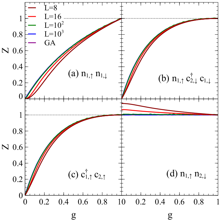
As the system size increases, renormalization factors, in the new approximation gradually approach the GA results, as illustrated in Fig. 3 and Fig. 4 on four typical operators in the half-filled case. Results deviating from half-filling are not shown as both methods are quite close to GWF results(e.g. see Ref [42] for the nonhalf-filling behavior of GA). From Fig. 3 we immediately see noticeable finite size effects for AA. It converges quickly as system size increases. At a system size of both AA and GA are nearly indistinguishable from each other. To provide a more quantitative measure on the asymptotic behavior of the new approximation, we present the system size dependence of the relative differences of renormalization factors between AA and GA in Fig. 4. The manifest linear dependence between these two quantities provides solid support on the conclusion that the new approximation asymptotically approaches GA in its infinite lattice limit. This might also suggest that the single band Gutzwiller approximation is quite an unexpectedly stable limit for the Gutzwiller wavefunction formalism with a site-wise local Gutzwiller projector.

IV An attempt to apply the new approximation to multiband systems
Thus far, we have applied the new approximation to single band systems and compared it against GA and other benchmark calculations. Encouraged by the limited success, we would like to generalize it to multiband systems which are physically more interesting and relevant to real problems. The simplest way to do so is to rewrite the Gutzwiller projector in terms of multi-orbital particle number operators[33], and to follow Eq. 18 to Eq. 23 to impose overall physical constraints. Unfortunately, this is not successful due to the very fact that the proposed approximation itself does not automatically preserve the correct total number of electrons in the system except for the single band case. Indeed, there is no guarantee that relevant physical constraints can be automatically preserved with such a simple and arbitrary wavefunction coefficient averaging scheme. It is a bit of luck that it does work out for single band systems.
However, this is not the excuse for us to give up the whole idea as it does provide us with a candidate recipe to define the renormalization factor for any operator. If we could look into the issue of failure a bit closer and at the same time fill us with confidence that the idea of averaging does work well on single band systems, we might come up with the following interpretation on the validity of the scheme: the averaging procedure does capture part of the correlation physics by giving reduced hopping or onsite double occupancy, etc., but it might describe correlation physics only qualitatively right in generic cases. One way to improve its quality requires more degrees of freedom to enable adjusting the way how the averaging can be carried out. This is actually quite similar to the logic Bunemann et. al. followed in deriving the multiband Gutzwiller approximation[33][32]. There, a set of orbital-wise fugacity parameters are introduced into the Gutzwiller trial wavefunction as adjustable parameters to ensure that the orbital occupations take the values evaluated with the noninteracting wavefunction[33], or fulfill some constraints of similar nature in case the local Gutzwiller projector is more general than involving only particle operators[36][38]. Their purpose to choose these constraints is for mathematical convenience to enable a rigorous Feynmann diagrammatic expansion to the total energy expectation value evaluated with the Gutzwiller trial wavefunction. Similarly, we will introduce the fugacity parameters into the trial wavefunction and impose other more reasonable physical constraints than creating a connection with information from the noninteracting wavefunction. We will use these fugacity parameters to calculate the renormalization factors defined through averaging. From a statistical point of view, these fugacity parameters define a weight on each wavefunction coefficient. Thus the renormalization factors are defined not as a simple averaging, but as a weighted averaging instead. With a careful choice of weights, a concept readily borrowed from the statistics theory, more reasonable renormalization factors are anticipated to make this new approximation useful. Specifically, we introduce into the trial wavefunction of Eq. 2 a local weighting operator
| (31) |
where is site index, denotes each local correlated orbital and is the weight of that state. Now the Gutzwiller trial wavefunction to be used in defining the renormalization factors is
| (32) |
Note, this wavefunction is not supposed to be used to evaluate physical expectation values of any operator. They are evaluated with Eq. 2 directly, and are thus unique given a Gutzwiller parameter . Of course, the choice of the weighting operator, is very flexible, depending on what kind of physical properties one decides to preserve. In case of a Hydrogen dimer described by a large basis set of 6-311G and to be studied here, we use Eq. 31 to ensure correct total number of electrons in the dimer system. The correlated orbital is chosen to be while other orbitals are treated uncorrelated. With these enhanced definitions, the whole averaging formalism can be written out and can be determined analytically as a function of . Details of the calculation are given in Appendix B. Rather unexpectedly, such a slightly modified averaging scheme gives an exact description on the multiband Hydrogen dimer system within a Gutzwiller trial wavefunction. Besides the nice agreement, one might appreciate a piece of physics embedded in the current approximation. We found that the fugacity parameter has two solutions. One solution gives orbital occupations identical to those of the underlying noninteracting wavefunction, a scenario adopted in the multiband GA formalism, and the other gives the correct orbital occupation in the Gutzwiller trial wavefunction. The coincidence of the solutions to the assumption underlying the multiband GA formalism might hint that the weighted version of the new approximation is intimately related with the multiband GA formalism that Bunemann et. al derived, just like AA to GA in the single band case. This fact might also speak loud that the new approximation introduced in this work could perform better than GA in capturing the strong correlation physics inherent in the Gutzwiller wavefunction formalism.
V Conclusion
In sum, we have introduced a very simple yet effective approximation towards the Gutzwiller wavefunction formalism. The simplicity is easily seen by noting that the renormalization factor of an operator is obtained through a direct average over nonvanishing coefficients of a Gutzwiller wavefunction constructed with a density-density type Gutzwiller projector. The effectiveness is supported by the agreement between the new approximation and GA, a well-studied approximation towards the Gutzwiller wavefunction formalism, in the infinite lattice limit of single band systems. Thus the current approximation provides a new perspective towards GA and its underlying assumptions. The proof showing their mutual relationship in Appendix A clearly reveals the grand canonical ensemble nature of GA, which readily prevents it from being applied to finite systems. This very nature of GA also shows itself in the counting argument interpretation of GA[32] but is not clear from the diagram based formulation[33]. In this work, several numerical instances are provided to compare the performance of the new approximation and GA, and to show the asymptotic agreement between these two schemes.
Although it shows an improved performance than GA in single band systems, the naive averaging, however, does not capture the double occupancy and other subtle physical quantities well enough. It also leads to the failure to reach the correct local orbital occupation in a Hydrogen dimer described with a large basis set, the simplest multiband system to be studied. All these can be improved however, at least partially, by introducing more fugacity parameters and physical constraints into the scheme. For example, a simple modification of introducing a weighting operator like Eq. 31 nicely fixes the multi-orbital Hydrogen dimer problem. Actually, such a simple problem indicates a possible close relation between the weighted averaging scheme and the multiband GA formalism. With a more carefully designed weighting factor and more physical constraints included in the formalism, the performance of the current approximation could be systematically improved to reach that of the Gutzwiller wavefunction formalism, with which the current approximation is built to match.
This new idea is applied most conveniently towards Gutzwiller trial wavefunction with its Gutzwiller projector commuting with number operators. Such a density-density type Gutzwiller projector (d-GPJ) might sound inferior than a more generic Gutzwiller projector (g-GPJ) defined with a general interaction operator to describe local correlation effects[36]. This might cast doubt on the ultimate usefulness of the current scheme to describe real systems. We have to admit that more variational degrees of freedom introduced in g-GPJ are able to give ground state energy. But we also believe that d-GPJ might perform with close quality as g-GPJ. It might also have an additional advantage of being more convenient in its implementation in practice. To fill us with some confidence first, we might find a successful application of d-GPJ in capturing the correct physics. Actually, such a Gutzwiller trial wavefunction has been applied to the Hubbard model and leads to the well-known t-J Hamiltonian in the strong correlation limit[29]. The t-J Hamiltonian, as well as the Heisenberg Hamiltonian as its special case, is the main working horse towards strong correlation limit and spin dynamics. Second, we believe that g-GPJ can only be treated in the multiband GA level in practice. Thus a much fairer comparison would be between the multiband GA and the current scheme, to compare which one is able to perform better. Then, the answer is clear that no party wins over the other for sure. One motivation to develop the formalism involving g-GPJ might be because GA from d-GPJ has to assume , a serious limitation in applying GA to multiband systems[33]. While GA from g-GPJ has this constraint removed, it still adopts constraints of similar nature in its derivation in order to carry out a Feynmann diagrammatic expansion[36]. Thus, how far multiband GA can be free from this constraint is unknown to us. In the new approximation introduced in this work, however, local orbital renormalization inherently exists which necessarily gives a local orbital occupation differring from its noninteracting value. One might systematically introduce more and more physical constraints into the formalism to help guide its outcome to be more and more physical. One more advantage of the current scheme against GA is that it is readily applied to Gutzwiller projectors with nonlocal density-density correlations. This fact is quite easy to notice although its practical implementation might be an issue.
Acknowledgements.
We are grateful to J. Bunemann and J. Schmalian for helpful discussions and valuable suggestions. This work is supported by the U.S. Department of Energy, Office of Basic Energy Sciences, Division of Materials Sciences and Engineering. Ames Laboratory is operated for the U.S. Department of Energy by Iowa State University under Contract No. DE-AC02-07CH11358.VI APPENDIX A: FROM THE NEW APPROXIMATION TO THE GUTZWILLER APPROXIMATION ON A SINGLE BAND SYSTEM
To establish a connection between these two approximations, let’s consider the renormalization coefficient for with site indices . Here denotes a spin-orbital composite state. Following the spirit leading to Eq. 18 to Eq. 20, one can write down and for as
| (33) | ||||
| (34) |
Here and denote a complete set of occupation configuration on the whole lattice, denotes the factor at site with local Fock state . In order to reach GA, let’s first relax the constraints, and note the following relations hold
| (35) | ||||
| (36) |
with total number of lattice sites and dimensionality of the local Fock space. We thus have
| (37) |
This expression for is only intermediate and not fully consistent, as one can see that fails to vanish as variational parameters in the standard Gutzwiller projector approaches 0.
Now let us introduce another approximation that the probability of finding a given Fock space occupation is a product of probabilities of finding the specific occupation configuration on each lattice site, or namely,
| (38) | ||||
| (39) |
where denote the probability to find a Fock state on site for the trial and noninteracting wavefunction respectively. This is too big a step forward as is normally not decomposeable on lattice sites. This approximation can be validated only in the infinite spatial dimension limit[43], which also underlies the Gutzwiller approximation. With this approximation, it is reasonable to assume
| (40) |
for the Gutzwiller trial wavefunction defined in Eq. 2 by noting that the local projection operator is site-wise. Feed Eq. 40 into Eq. 37 and we get
| (41) |
with
| (42) |
A mean-field type approximation is now introduced for terms involving by replacing those terms with their averages. Again, in the infinite spatial dimension limit and under some convenience conditions, can be expressed in terms of local occupancy, on each local state , as
| (43) |
Then there are two averages needed to be calculated,
| (44) | ||||
| (45) | ||||
| (46) |
and
| (47) |
Here is the dimensionality of the local Fock space. The prefactor in Eq. 46 accounts for the fact that must not contain state in it. Plug Eq. 46 and Eq. 47 back to Eq. 42 and one recovers the standard GA definition of given in Eq. 5.
VII APPENDIX B: THE NEW APPROXIMATION WITH WEIGHTED AVERAGE APPLIED ON THE MULTIBAND H DIMER SYSTEM
To make things simple, let’s consider a local basis set composed of one correlated orbital, denoted as and uncorrelated orbitals to describe the H-dimer, all defined as Wannier functions such that they are orthogonal to each other within and between sites. A molecular orbital is thus generically created via operator
| (48) |
where creates an electron at site and orbital with spin or, . The coefficients satisfy the normalization condition
| (49) |
with translational invariance implicitly assumed. That the cross terms contributing to the normalization vanish comes from the fact that each atomic orbital is a Wannier function, as mentioned at the beginning of this appendix. Eq. 49 also expresses the electron conservation condition, ensuring each site has half an electron with a specific spin. The noninteracting Hartree-Fock wavefunction can be expressed as
| (50) |
for the H dimer, and the Gutzwiller wavefunction is defined as
| (51) |
with the Gutzwiller parameter. Expectation value w.r.t the Gutzwiller wavefunction for any operator can be straightforwardly evaluated. Specifically, for particle occupations, there are
| (52) | ||||
| (53) |
Obviously, it is easy to test that they satisfy the electron conservation condition, Eq. 49, with help of that constraint.
For the current approximation with weighted average enhancement, the local weighting operator is chosen as
The expectation value for an operator is considered from its denominator, wavefunction normalization, and its numerator respectively. For the normalization factor there is
| (54) |
with the usual combinatorial number choosing elements out of elements. In the numerator of the renormalization factor in Eq. 54, each term has clear physical interpretation. corresponds to two electrons occupying orbitals on the same site, has the two electrons take orbitals on different sites, is related to Fock states with only one electron in orbitals, while the last term corresponds to Fock states with no orbital. The terms in the denominator of the above prefactor are obtained by ignoring the variational parameter What is left acts as the weight to each term in the numerator, a necessary step to normalize a weighted average. Similarly, one can write down the numerator of the expectation value of an operator. For electron occupations, they are
| (55) | ||||
| (56) |
The constraint of conserved electron occupation on a H dimer requires
| (57) |
Feed Eq. 54, Eq. 55 and Eq. 56 into Eq. 57 and solve for and one ends up with two solutions
| (58) | ||||
| (59) |
Interestingly, both these two solutions have clear physical interpretations. corresponds to the case where the correlated system has the same local orbital occupation as the underlying noninteracting wavefunction, which is what Bunemann’s multiband Gutzwiller approximation starts with. The nontrivial solution of Eq. 59 to gives the correct charge occupation as the rigorous Gutzwiller wavefunction. One can readily verify this fact by inserting the solution Eq. 59 back to the expressions for and and take the constraint of Eq. 49. Actually, one can further verify that this nontrivial solution renders correct expressions for any one and two body operators of the H dimer system.
References
- [1] P. Fazekas, Lecture Notes on Electron Corrrelation and Magnetism, 2nd ed. (World Scientific, Singapore, 2003)
- [2] P. W. Anderson, The Theory of Superconductivity in the High-Tc Cuprate Superconductors, 1st ed. (Princeton University Press, New Jersey, USA, 1997)
- [3] P. Coleman, Heavy Fermions: electrons at the edge of magnetism, in Handbook of Magnetism and Advanced Magnetic Materials, Vol 1: Fundamentals and Theory, ed. by H. Kronmuller and S. Parkin, 1st ed. (J. Wiley and Sons, New Jersey, USA, 2007) pp. 95–148
- [4] D. N. Basov, R. D. Averitt, D. van der Marel, M. Dressel, and K. Haule, Rev. Mod. Phys. 83, 471 (2011)
- [5] O. Parcollet, G. Biroli, and G. Kotliar, Phys. Rev. Lett. 92, 226402 (2004)
- [6] J. Liu, J. Schmalian, and N. Trivedi, Phys. Rev. Lett. 94, 127003 (2005)
- [7] A. L. Fetter and J. D. Walecka, Quantum Theory of Many Particle Systems, 1st ed. (Dover Publications, New York, US, 2003)
- [8] D. P. A. Chubukov and J. Schmalian, A Spin Fluctuation Model for d-wave Superconductors, in The Physics of Superconductors, ed. K.H. Benneman and J. B. Ketterson, 2nd ed. (Springer, Berlin, Germany, 2008) pp. 1349–1407
- [9] N. E. Bickers and D. J. Scalapino, Ann. Phys. 193, 206 (1989)
- [10] C. X. Chen and N. E. Bickers, Solid State Commun. 82, 311 (1992)
- [11] N. E. Bickers, in Theoretical Methods for Strongly Correlated Electrons, edited by D. Senechal, A. Tremblay, and C. Bour-bonnais (Springer-Verlag, New York, USA, 2004) p. 237
- [12] J. C. Bonner and M. E. Fisher, Phys. Rev. 135, A640 (1964)
- [13] J. E. Hirsch, R. L. Sugar, D. J. Scalapino, and R. Blankenbecler, Phys. Rev. B 26, 5033 (1982)
- [14] A. Georges, G. Kotliar, W. Krauth, and M. J. Rozenberg, Rev. Mod. Phys. 68, 13 (1996)
- [15] G. Kotliar, S. Y. Savrasov, G. Pálsson, and G. Biroli, Phys. Rev. Lett. 87, 186401 (2001)
- [16] T. Maier, M. Jarrell, T. Pruschke, and M. H. Hettler, Rev. Mod. Phys. 77, 1027 (2005)
- [17] K. G. Wilson, Rev. Mod. Phys. 47, 773 (1975)
- [18] R. Bulla, T. A. Costi, and T. Pruschke, Rev. Mod. Phys. 80, 395 (2008)
- [19] S. R. White, Phys. Rev. Lett. 69, 2863 (1992)
- [20] J. Zeng, Quantum Mechanics, Volume I, 3rd ed. (Science Press, Beijing, China, 2000)
- [21] P. Hohenberg and W. Kohn, Phys. Rev. 136, B864 (Nov 1964), http://link.aps.org/doi/10.1103/PhysRev.136.B864
- [22] W. Kohn and L. J. Sham, Phys. Rev. 140, A1133 (Nov 1965), http://link.aps.org/doi/10.1103/PhysRev.140.A1133
- [23] P. W. Anderson, G. Baskaran, Z. Zou, and T. Hsu, Phys. Rev. Lett. 58, 2790 (1987)
- [24] P. W. Anderson, Science 235, 1196 (1987)
- [25] M. C. Gutzwiller, Phys. Rev. Lett. 10, 159 (1963)
- [26] J. Hubbard, Proc. Roy. Soc. A 276, 238 (1963)
- [27] M. C. Gutzwiller, Phys. Rev. 134, A923 (1964)
- [28] J. Spałek, Phys. Rev. B 37, 533 (1988)
- [29] e. a. A. P. Balachandran, Hubbard model and anyon superconductivity (World Scientific Publishing Co., Singapore, 1990)
- [30] D. Vollhardt, Rev. Mod. Phys. 56, 99 (1984)
- [31] K. K. Tohru Ogawa and T. Matsubara, Prog. Theor. Phys. 53, 614 (1975)
- [32] J. Bumenann, Eur. Phys. J. B 4, 29 (1998)
- [33] J. Bunemann, F. Gebhard, and W. Weber, Journal of Physics: Condensed Matter 9, 7343 (1997)
- [34] W. Metzner and D. Vollhardt, Phys. Rev. Lett. 62, 324 (1989)
- [35] W. Metzner and D. Vollhardt, Phys. Rev. B 37, 7382 (1988)
- [36] J. Bünemann, W. Weber, and F. Gebhard, Phys. Rev. B 57, 6896 (1998)
- [37] T. Okabe, J. Phys. Soc. Japan 65, 1056 (1996)
- [38] M. Fabrizio, Phys. Rev. B 76, 165110 (2007)
- [39] W. F. Brinkman and T. M. Rice, Phys. Rev. B 2, 4302 (1970)
- [40] V. Anisimov, I. Nekrasov, D. Kondakov, T. Rice, and M. Sigrist, The European Physical Journal B - Condensed Matter and Complex Systems 25, 191 (2002), ISSN 1434-6028, http://dx.doi.org/10.1140/epjb/e20020021
- [41] I. Shavitt and R. J. Bartlett, Many-Body Methods in Chemistry and Physics: MBPT and Coupled-Cluster Theory, 1st ed. (Cambridge University Press, Cambridge, UK, 2009)
- [42] W. Metzner and D. Vollhardt, Phys. Rev. B 37, 7382 (1988)
- [43] This statement can be formally argued in the following way. Introduce a bosonic operator for projecting out a Fock state on each lattice site and the occupation probability for a given occupation configuration can be expressed as . This expression is then decomposeable in site indices in the infinite dimension limit.