Planck 2015 results. XXVII. The Second Planck Catalogue of Sunyaev-Zeldovich Sources
Abstract
We present the all-sky Planck catalogue of Sunyaev-Zeldovich (SZ) sources detected from the 29 month full-mission data. The catalogue (PSZ2) is the largest SZ-selected sample of galaxy clusters yet produced and the deepest all-sky catalogue of galaxy clusters. It contains 1653 detections, of which 1203 are confirmed clusters with identified counterparts in external data-sets, and is the first SZ-selected cluster survey containing confirmed clusters. We present a detailed analysis of the survey selection function in terms of its completeness and statistical reliability, placing a lower limit of 83% on the purity. Using simulations, we find that the estimates are robust to pressure-profile variation and beam systematics, but accurate conversion to requires. the use of prior information on the cluster extent. We describe the multi-wavelength search for counterparts in ancillary data, which makes use of radio, microwave, infra-red, optical and X-ray data-sets, and which places emphasis on the robustness of the counterpart match. We discuss the physical properties of the new sample and identify a population of low-redshift X-ray under-luminous clusters revealed by SZ selection. These objects appear in optical and SZ surveys with consistent properties for their mass, but are almost absent from ROSAT X-ray selected samples.
Key Words.
cosmology: observations – galaxies: clusters: general – catalogues1 Introduction
This paper is one of a set associated with the 2015 Planck11 1 Planck (http://www.esa.int/Planck) is a project of the European Space Agency (ESA) with instruments provided by two scientific consortia funded by ESA member states and led by Principal Investigators from France and Italy, telescope reflectors provided through a collaboration between ESA and a scientific consortium led and funded by Denmark, and additional contributions from NASA (USA). full mission data release and describes the production and properties of the legacy catalogue of Sunyaev Zeldovich sources (PSZ2).
In the framework of hierarchical structure formation, peaks in the cosmological density field collapse and merge to form gravitationally bound haloes of increasing mass (Peebles 1980). The galaxy clusters are the most massive of these bound structures and act as signposts for the extrema of the cosmological density field on the relevant scales. The evolution of galaxy cluster abundance with mass and redshift is thus a sensitive cosmological probe of the late-time universe, providing unique constraints on the normalisation of the matter density fluctuations, , the mean matter density, , the density and equation of state of the dark energy field, and , as well as constraining some extensions of the minimal cosmological model, such as massive neutrinos, and non-standard scenarios such as modified gravity (see eg: Borgani & Kravtsov 2009; Allen et al. 2011). In recent years, cluster data from the microwave through to the X-ray have been used to constrain cosmological parameters (Vikhlinin et al. 2009b; Rozo et al. 2010; Hasselfield et al. 2013; Benson et al. 2013; Planck Collaboration XX 2014; Zu et al. 2014).
Galaxy clusters are multi-component objects composed of dark matter, which dominates the mass, stars, cold gas and dust in galaxies, and a hot ionised intra-cluster medium (ICM). These different components make clusters true multi-wavelength objects. The galaxies emit in the optical and infrared. The ICM, which is the majority of the baryonic material by mass, emits in the X-rays via thermal bremsstrahlung and line emission, and energy-boosts cosmic microwave background photons via inverse Compton scattering.
This last effect, the thermal Sunyaev Zeldovich (SZ) effect (Sunyaev & Zeldovich 1970; Sunyaev & Zeldovich 1980), imprints a redshift-independent spectral distortion on the cosmic-microwave background (CMB) photons reaching us along the line of sight to the cluster. This results in an increase in intensity at frequencies above 220 GHz, and a decrease in intensity at lower frequencies. The Planck High-Frequency Instrument (HFI) is unique in providing high-precision data for both the increment and the decrement across the whole sky.
The utility of a cluster survey for cosmological work depends on our ability to determine accurately its selection function and to obtain unbiased measurements of cluster mass and redshift. The first cluster surveys consisted of galaxy overdensities identified by eye from photographic plates (Abell 1958). The construction of large optical catalogues improved significantly with the data from the SDSS (Koester et al. 2007), whose five photometric bands have allowed robust photometric classification of red-sequence cluster galaxies and accurate photometric redshifts to across 1/4 of the sky (Hao et al. 2010; Szabo et al. 2011; Wen et al. 2009; Rykoff et al. 2014). These catalogues now typically contain clusters and provide cluster richness as an observable that correlates with mass with an intrinsic scatter of about % (Rozo & Rykoff 2014).
Construction of X-ray cluster surveys is now a mature activity, with several catalogues now available based on all-sky data from the ROSAT satellite, alongside additional catalogues of serendipitous detections from pointed observations (Ebeling et al. 1998; Böhringer et al. 2004; Reiprich & Böhringer 2002; Ebeling et al. 2010; Piffaretti et al. 2011; Burenin et al. 2007; Mehrtens et al. 2012). The most basic X-ray survey observable, the X-ray luminosity measured within 22 2 is the cluster-centric distance within which the mean density is 500 times the critical density of the Universe at the cluster redshift., has been shown correlate with mass with intrinsic scatter of about % (Pratt et al. 2009). Observables with lower intrinsic scatter against mass can be defined when pointed X-ray follow-up information is available, including the core-excised X-ray luminosity (Maughan 2007; Pratt et al. 2009) and , the product of the gas mass and the core-excised spectroscopic temperature (Kravtsov et al. 2006; Vikhlinin et al. 2009a; Mahdavi et al. 2013). While X-ray surveys are unique in their purity, they do suffer from selection biases that favour low-redshift systems, due to flux limitations, and dynamically relaxed clusters with an X-ray bright cooling core (Eckert et al. 2011; Schuecker et al. 2003; Vikhlinin et al. 2009b; Chen et al. 2007).
SZ surveys offer a different window on the cluster population: their selection function flattens towards higher redshifts, providing a nearly mass-limited census of the cluster population at high redshift, where abundance is strongly sensitive to cosmological parameters (Carlstrom et al. 2002; Planck Collaboration XXIX 2014). The SZ survey observable is the spherically integrated Comptonisation parameter, , which is related to the integrated electron pressure and hence the total thermal energy of the cluster gas. It is also expected to correlate with mass with a low intrinsic scatter and little dependence on the dynamical state of the cluster (eg: da Silva et al. 2004; Kay et al. 2012; Hoekstra et al. 2012; Planck Collaboration Int. III 2013; Sifón et al. 2013).
The spherically-integrated pressure profiles of X-ray and SZ clusters have been observed to follow a near universal profile with little dispersion (Arnaud et al. 2010; Planck Collaboration Int. V 2013), permitting the detection of clusters with a matched multi-frequency filter based on some assumed pressure profile (Herranz et al. 2002; Melin et al. 2006a). Samples constructed this way have well understood selection functions, though discrepancies due to profile mismatch or contaminating infra-red emission may still be present to some level. Large SZ surveys have only appeared recently, with catalogues of order clusters released by the Atacama Cosmology Telescope (Hasselfield et al. 2013), the South Pole Telescope (Reichardt et al. 2013) and Planck satellite collaborations.
This is the third all-sky catalogue produced from Planck SZ data. The early Sunyaev-Zeldovich (ESZ) catalogue presented 189 clusters detected from 10 months of survey data (Planck Collaboration 2011), while the PSZ1, the full-sky catalogue assembled from the nominal mission data, presented 1227 cluster candidates detected from 15.5 months of data (Planck Collaboration XXIX 2014). This paper presents 1653 candidates detected from the full mission survey of 29 months. 1203 of these have been confirmed in ancillary data, and 1094 have redshift estimates. The PSZ2 expands the scope and sensitivity of the SZ view of galaxy clusters by substantially increasing the number of lower mass clusters available for study. It is also expected to contain many new, as yet unconfirmed, high-redshift clusters. We report on the construction and characterisation of the catalogue, presenting the survey selection functions and a compilation of multi-wavelength ancillary information including redshifts. We also briefly discuss the physical properties of the sample.
This paper is organised as follows. In Sect. 2 we summarise the three extraction algorithms used to build the catalogue, focussing on the changes in the algorithms since they were used to construct the PSZ1. In Sect. 3 we describe the construction of the catalogue. In Sect. 4 we present the survey selection functions (completeness and statistical reliability) and the complementary approaches used to estimate them, while in Sect. 5 we discuss and validate the estimation of the parameters, both blindly and when using prior information, and we compare the consistency of the new catalogue with the PSZ1 in Sect. 6. In Sect. 7 we report on the search for multi-wavelength counterparts in ancillary catalogues and follow-up observations. Finally we present the physical properties of the sample in Sect. 8 and conclude in Sect. 9. A full description of the available data products is given in Appendix D
2 Extraction Algorithms
The SZ detection and parameter estimation algorithms used to construct the PSZ2 extend and refine those used to construct the PSZ1. In this section we recall the principles of the three algorithms. The refinements of each algorithm since the PSZ1 release are detailed in Appendix C. Two of the algorithms (MMF1 and MMF3) are based on the same technique (Matched Multi-filters) but have been implemented independently33 3 The MMF numbers were given after the comparison of twelve algorithms in an earlier phase of the Planck mission (Melin et al. 2012). MMF1 and MMF3 were respectively the first and third algorithm based on Matched Multi Filters to enter the comparison. The third one (PwS for PowellSnakes) relies on Bayesian inference.
2.1 Matched Multi-filters: MMF1 and MMF3
The matched filtering technique was first proposed for SZ studies by Haehnelt & Tegmark (1996). It was subsequently developed by Herranz et al. (2002) and Melin et al. (2006b) for SZ cluster extraction in multifrequency data sets such as Planck. The method was later adopted by the SPT and ACT collaborations (Staniszewski et al. 2009; Marriage et al. 2011).
We model the vector of map emission at each frequency , at a given position on the sky as
| (1) |
where is the signal vector describing the spatial distribution at each frequency of the SZ emission from a cluster with angular size , is the total astrophysical and instrumental noise. The frequency component of the signal vector is the normalized cluster profile (Arnaud et al. 2010) convolved by the Planck beams and scaled with the characteristic frequency dependance of the thermal SZ effect: . is the cluster scale radius, which is related to through the concentration parameter by . The Matched Multi-filter allows us to recover an unbiased estimate of the central Comptonization parameters with minimal variance :
| (2) |
where
| (3) |
with
| (4) |
being the cross-channel power spectrum matrix of the maps. It is effectively the noise matrix for the MMF, because the tSZ is small compared to other astrophysical signals, and is estimated directly from the maps.
The MMF algorithms first divide each Planck all-sky map in 640/504 tangential maps (14.66/10 degrees on a side) for MMF1 /MMF3 respectively. Each set of tangential maps is filtered by with the assumed cluster size varying from =0.8 to 32 arcmin. We then locate peaks in the filtered maps above a S/N threshold of four. The locations of the peaks give the positions of our cluster candidates. These are then merged into a single all-sky catalogue by merging candidates separated by less than 10 arcmin. For MMF3, we performed a second step by creating sets of smaller rectangular frequency maps centered on the cluster candidates identified in the first step. We re-apply the MMF on these centred tangential maps which allows a better estimation of the background. During the second step, the sizes and fluxes are estimated more precisely. This second step is only performed for MMF3 because the overlap of the tangential maps in the first step is small with compared to MMF1and PwS.
We define the blind cluster size as the filter scale that maximizes the S/N at the location of the cluster candidate and the blind flux is defined as the corresponding parameter. We then define the integrated blind flux as:
| (5) |
Each of the algorithms produces probability distributions in the (, ) plane for each detection, marginalising over the parameters for the centre of the cluster, which possess a Gaussian likelihood. The algorithms also return an estimate of the radial position uncertainty, from the position likelihood.
Although the two implementations of the MMF are quite close, they produce noticeably different catalogues because the extraction is very sensitive to the estimation of the background (Eq. 4). Both the size adopted for the tangential maps and the details of the estimation of the matrix impact the S/N and hence which peaks are detected.
2.2 PowellSnakes (PwS)
PowellSnakes (PwS) is a fast, fully Bayesian, multifrequency detection algorithm designed to identify and characterize compact objects buried in a diffuse background as described in Carvalho et al. (2009); Carvalho et al. (2012). PwS operates using about 2800 square patches of 14.66 degree on a side, in order to ensure highly redundant sky coverage. PwS detects candidate clusters and at the same time computes the evidence ratio and samples from the posterior distributions of the cluster parameters. Then, it merges the sub-catalogues from each patch map and applies criteria for acceptance or rejection of the detection, as described in Carvalho et al. (2012). Priors may be provided for the position, integrated flux and radius of the clusters. For cluster detection, we apply flat priors on the position and non-informative priors in the radius and integrated flux, as determined using Jeffrey’s method. PwS uses a calibration of the cross-power spectrum that uses an iterative scheme to reduce the contamination of the background by the SZ signal itself. This makes PwS particularly robust to small changes in the background.
3 Catalogue Construction
The main catalogue is constructed by combining the detections made by the three methods into a union catalogue, while merging the detections made by multiple more than one method. Half of the detections in this union are also in the intersection catalogue, defined as those detections made by all three codes simultaneously. This section describes the technical details of the construction of these catalogues.
3.1 Pipeline
| Channel | FWHM | |
|---|---|---|
| 100 | 9.659 | 103.416 |
| 143 | 7.220 | 144.903 |
| 217 | 4.900 | 222.598 |
| 353 | 4.916 | 355.218 |
| 545 | 4.675 | 528.400 |
| 857 | 4.216 | 776.582 |
The SZ catalogue construction pipeline is shown in schematic form in Fig. 1 and largely follows the process used to build the PSZ1. The Planck data required for the construction of the catalogue comprises the HFI maps, point source catalogues for each of the HFI channels, effective frequencies and beam widths per HFI channel as shown in Table 1, survey masks based on dust emission as seen in the highest Planck channels, and the catalogue of extended galactic cold-clump detections.
The HFI maps are pre-processed to fill areas of missing data (typically a few pixels), or areas with unusable data, specifically bright point sources. Point sources with S/N in any channel are masked out to a radius of , using a harmonic infilling algorithm. This prevents spurious detections caused by Fourier ringing in the filtered maps used by the detection algorithms. As a further guard against such spurious detections, we reject any detections within of a filled point source. We have verified that this treatment reduces spurious detections due to bright point sources to negligible levels in simulations, while reducing the effective survey area by just 1.4% of the sky. Together with the 15% galactic dust and Magellanic cloud mask, this defines a survey area of 83.6% of the sky.
After infilling, the three detection codes produce individual candidate catalogues down to a threshold S/N . The catalogues are then merged to form a union catalogue, using the dust and extended point source masks discussed above to define the survey area. The merging procedure identifies the highest S/N detection as the reference position during the merge: any detections by other codes within 5 arcmin are identified with the reference position. The reference position and S/N are reported in the union catalogue.
PwS can produce a small number of high-significance spurious detections associated with galactic dusty emission. We apply an extra cut of PwS-only detections at S/N where the spectrum has a poor goodness-of-fit to the SZ effect, .
We also remove five PSZ2 detections that match PSZ1 detections confirmed to be spurious by the PSZ1 follow-up program (these were the ones that we re-detected: there were many more confirmed spurious detections from the program).
Finally the sample is flagged to identify the various sub-samples discussed in Sect. 3.3. The most important of these flags is discussed in the next section.

3.2 Infra-red spurious detections
Cold compact infra-red emission, particularly that due to galactic cold-clumps, can lead to high-significance spurious detections. We identify these detections by searching for 7 arcmin matches with the Planck cold-clump catalogue (C3PO), or with PCCS2 detections at both 545GHz and 857GHz. This matching radius was chosen because it is the typical size of a Planck detected cold-clump (Planck Collaboration XXVIII 2015).
318 raw union detections match these criteria. They tightly follow the distribution of galactic emission (see Fig. 2), such that if the 65% galactic dust mask (used for cluster cosmology ) is used to define the sample instead of the 85% dust mask, the number of IR-matched raw detections drops to 40. For the high-purity sample formed from the intersection of all three codes, the numbers are 82 and 13 for the 85% and 65% dust masks respectively. Some high latitude spurious candidates remain. To minimise the effect of these probably spurious detections on the catalogue, we delete them.
We have retained in the sample all 15 confirmed clusters that match these criteria. These IR contaminated clusters represent about % of the total confirmed clusters in the PSZ2. In the catalogue, we define a flag, IR_FLAG, to denote the retained clusters that match these criteria. They can be expected to have heavily contaminated SZ signal.
A small fraction of the unconfirmed detections deleted due to IR-contaminations may have been real clusters. Assuming that optical and X-ray confirmation is unbiased with regard to the presence of IR emission, we estimate these deletions to bias our completeness estimates by less than 1%.

3.3 Catalogue sub-samples
The union catalogue can be decomposed into separate sub-samples, defined as the primary catalogues of the three individual detection codes (PwS,MMF1,MMF3), as well as into unions and intersections thereof. The intersection subsample of candidates detected by all three algorithms can be used as a high-reliability catalogue with less than spurious contamination outside of the galactic plane (see Sect. 4.6).
3.3.1 The Cosmology Catalogues
We constructed two cluster catalogues for cosmology studies from the MMF3 and the intersection sub-samples respectively. For these catalogues, our goal was to increase as much as possible the number of detections while keeping contamination negligible. A good compromise is to set the S/N threshold to 6 and apply a 65% galactic and point source mask as in our 2013 cosmological analysis (Planck Collaboration XX 2014). In this earlier paper, our baseline MMF3 cosmological sample was constructed using a threshold of 7 on the 15.5 month maps, which is equivalent to 8.5 on the full mission maps. Estimations from the QA (Fig. 11) suggest that our 2014 intersection sample should be % pure for a threshold of 6.
The MMF3 cosmological sample contains 439 detections with 433 confirmed redshifts. The intersection cosmological sample contains 493 detections with 479 confirmed redshifts. Assuming that all detections having VALIDATION flag greater than zero are clusters, the empirical purity of our samples are % for MMF3 and % for the intersection. Note that the intersection sample contains more clusters than the MMF3 sample for the same S/N threshold. This is expected since the definition of the S/N for the intersection sample is to use the highest value from the three detection methods.
The completeness is also a crucial piece of information. It is computed more easily with the single method catalogue for which the analytical error-function (ERF) approximation can be used (as defined in Planck Collaboration XXIX 2014). In Sect. 4.3 and in Planck Collaboration XXIV (2015), we show that this analytical model is still valid for the considered threshold. For the intersection sample, we rely on the Monte-Carlo estimation of the completeness described in Sect. 4.2.
These two samples are used in the cosmology analysis of Planck Collaboration XXIV (2015). Detections that are included in either of the cosmology samples are noted in the main catalogue (see Appendix D).
3.4 Consistency between codes


| N | A | |||||
|---|---|---|---|---|---|---|
| MMF1 | MMF3 | 1032 | ||||
| MMF1 | PwS | 985 | ||||
| MMF3 | PwS | 1045 |
We construct the union sample using the code with the most significant detection to supply the reference position and S/N. This contrasts with the PSZ1, which used a pre-defined code ordering to select the reference position and S/N. In this section, we demonstrate the consistency of the detection characteristics of the codes for common detections, motivating this change in catalogue construction.
We fit the S/N relation between codes using the Bayesian approach described by Hogg et al. (2010) for linear fits with covariant errors in both variables. We consider the catalogue S/N values to be estimates of a true underlying variable, , with Gaussian uncertainties with standard deviation .
We relate the values for two different catalogues using a simple linear model
| (6) |
where we assume flat priors for the intercept , a flat prior on the arc-tangent of the gradient , such that . We also allow for a Gaussian intrinsic scatter between the values that includes any variation beyond the measurement uncertainty on . This is parameterised by with an uninformative prior .
We assume a fiducial correlation of between the S/N estimates of each code pair, which is typical of the correlation between the matched-multifrequency-filtered patches of each code. The fit results are shown in Table 2.
The S/N estimates from the three codes are compared in Fig. 3, which also shows the best fit relation. MMF1 produces noticeably weaker detection than the other two codes for the 14 very strong detections at S/N . Excluding these exceptional cases from the comparison, the best-fit relations between the S/Ns from each code show no significant deviations from equality between any of the codes.
There are a small number of highly significant outliers in the relation between PwS and the MMF codes. These are clusters imbedded in dusty regions where the different recipes for the filtered patch cross-power spectrum vary significantly and the likelihood assumptions common to all codes break down. PwS shows outlier behaviour relative to the other codes as its recipe is most different from the other codes.
Fig. 4 shows the consistency of the position estimates between the codes. The positions of MMF1 and MMF3 are more inconsistent with one another than any other code combination. The 67% bound on the MMF1- MMF3 separation is 1.34 arcmin, while for MMF1- PwS it is arcmin and for MMF3- PwS it is arcmin. This is consistent with the observation from the quality assessment that the PwS positions are the most robust (Sect. 4.4).

4 Selection Function
A necessary element of any cluster sample is the selection function that relates the detected sample to the underlying population of objects. The selection function comprises two complementary functions: the completeness, which defines the probability that a given real object will be detected; and the statistical reliability, also known as purity, which defines the probability that a given detection corresponds to a real object. As a function of underlying object attributes, the completeness is a function of underlying SZ observables, and . The reliability is a statistical function of detection attributes and is presented as a function of detection S/N.
4.1 Monte-Carlo Injection
The selection function is determined by the Monte-Carlo injection of simulated clusters into both real and simulated Planck maps. A common segment is the injection of cluster SZ signal. The cluster signal is assumed to be spherically symmetric and to follow a pressure profile similar to the generalised Navarro-Frenk-White (GNFW) profile assumed in the catalogue extraction.
To include the effects of system-on-system variation in the pressure distribution, we draw the spherically-averaged individual pressure profiles from a set of 910 pressure profiles from simulated clusters from the cosmo-OWLS simulations (Le Brun et al. 2014; McCarthy et al. 2014), an extension of the OverWhelmingly Large Simulations project (Schaye et al. 2010). These pressure profiles are empirical in the sense that they have not been fitted using a GNFW profile: the mean pressure is used within concentric radial shells (after the subtraction of obvious sub-structures) and the injected profiles are interpolated across these shells. The simulated clusters were selected for this sample by requiring that their mass be above the approximate limiting mass for Planck at that redshift. The ensemble of simulated profiles are shown in Fig. 5. Each profile is normalised such that the spherically integrated Y parameter matches the fiducial injected (,) parameters for the halo. The injected (,) are different for completeness and reliability simulations and each is discussed below.

Effective beam variation is an important consideration for the unresolved clusters at the intermediate and high redshifts of cosmological interest. The injected clusters are convolved with effective beams in each pixel including asymmetry computed following Mitra et al. (2011)
4.2 Completeness
The completeness is defined as the probability that a cluster with a given set of true values for the observables (,) will be detected, given a set of selection criteria. A good approximation to the completeness can be defined using the assumption of Gaussianity in the detection noise. In this case, the completeness for a particular detection code follows the error function (ERF), parametrised by a selection threshold and the local detection noise at the clusters radial size, (see the discussion in Planck Collaboration XXIX 2014). This approach is not suited to the union and intersection catalogues from Planck due to the difficulty in modelling correlations between detection codes. We determine the completeness by brute force: injecting and detecting simulated clusters into the Planck sky maps. This approach has the advantage that all algorithmic effects are encoded into the completeness, and the effects of systematic errors such as beam and pressure profile variation can be characterised. This approach also fully accounts for the non-Gaussianity of the detection noise due to foreground emission.
The injected (,) parameters are drawn from a uniform distribution in the logarithm of each variable, ensuring that our logarithmically spaced completeness bins have approximately equal numbers of injected sources.
As the completeness is estimated from injection into real data, injected sources can contribute to the detection noise. We therefore use an injection mode, as was the case for the PSZ1 completeness, where injected clusters are removed from the maps used to estimate the noise statistics. We also avoid superimposing injected clusters on top of one another, or on top of real data detections. Together, these ensure that the noise statistics for injected clusters are the same as for the real detections in the map.
We release as a product the Monte-Carlo completeness of the catalogues at thresholds stepped by 0.5 in S/N over the range S/N. Fig. 6 shows the completeness of the union and intersection catalogues as functions of input (,) and at representative values of , for three detection thresholds. The union and intersection catalogues are most similar at high S/N, where they match well except at small scales. Here the intersection catalogue follows the lower completeness of MMF1. This is due to an extra selection step in that code which removes spurious detections caused by point sources. The union and the intersection catalogues mark the upper and lower limits of the completeness values for the sub-catalogues based on the individual codes.
The completeness of the Planck cluster catalogue is robust with respect to deviations of the real SZ profiles of galaxy clusters from the one assumed by the algorithms for filter construction. To demonstrate this, we compare , the Monte-Carlo completeness for the MMF3 sample, using the cosmoOWLs profile variation prescription and effective beam variation, to , the semi-analytic ERF completeness. This comparison is shown in Fig. 7, where we show the difference between the two estimates as a function of and as well the individual completeness values as functions of for representative values of slices through the 2D completeness and show the difference.
The error function is a good approximation to the MC completeness for the cosmology sample, which uses a higher S/N cut and a larger Galactic mask than the full survey. The MC estimate corrects this analytic completeness by up to 20% for large resolved clusters, where is systematically less complete than the ERF expectation, primarily due to variation in the cluster pressure profiles. For unresolved clusters, the drop-off in is slightly wider than the ERF expectation, reflecting variation both of pressure profiles and of effective beams.
The impact of these changes in completeness on expected number counts and inferred cosmological parameters for the cosmology sample is analysed in Planck Collaboration XXIV (2015). The difference between the Monte-Carlo and ERF completeness results in a change in modelled number counts of typically % (with a maximum of 9%) in each redshift bin. This translates into a shift of the posterior peak for the implied linear fluctuation amplitude,.
The MC completeness is systematically lower than the analytic approximation for the full survey. One of the causes of this is galactic dust contamination, which is stronger in the extra 20% of the sky included in the full survey area relative to the cosmology sample area. This tends to reduce the S/N of clusters on affected lines of sight.
We note that this approach ignores other potential astrophysical effects that could affect the completeness. Radio emission is known to be correlated with cluster positions, potentially ‘filling in’ the SZ decrement, though recent estimates suggest that this effect is typically small in Planck data (Rodriguez-Gonzalvez et al. 2015). Departures of the pressure distribution from spherical symmetry may also affect the completeness, though this effect is only likely to be significat for nearby and dynamically disturbed clusters which may be large compared to the Planck beams. We test for some of these effects through external validation of the completeness in the next section, and explicitly through simulation in Sect. 4.5.
Another source of bias is the presence of correlated IR emission from cluster member galaxies. Planck Collaboration XXIII (2015) show that IR point sources are more numerous in the direction of galaxy clusters, especially at higher redshift, and contribute significantly to the cluster SED at the Planck frequencies. Initial tests, injecting clusters signal with the combined IR+tSZ spectrum of clusters observed by Planck Collaboration XXIII (2015), suggest that this reduces the completeness for unresolved clusters. Future work is warranted to characterise the evolution and scatter of this IR emission and to propagate the effect on completeness through to cosmological parameters.


4.3 External validation of the completeness
We validated our Monte-Carlo completeness calculation and our simple analytical ERF model by using the MCXC (Piffaretti et al. 2011) and SPT (Bleem et al. 2014) catalogues. The Planck detection threshold passes across the cluster distributions of these two samples. This is illustrated in Fig. 4 of Chamballu et al. (2012) for the MCXC. This allows us to characterize our completeness by checking if the fraction of detected clusters follows the expected probability distribution as a function of their parameters. For each cluster of the MCXC catalogue, we use the MMF3 algorithm to extract its flux and associated error at the location and for the size given in the x-ray catalogue. We then build the quantity , q being the detection threshold (here 4.5) and the noise of the filtered maps. We make the corresponding histogram of this quantity for all the clusters and for the clusters detected by MMF3. The ratio of the two histograms is an empirical estimate of the completeness. Results are shown in Fig. 8 for the MCXC (left) and the SPT (right) catalogues. For MCXC, the estimation is in good agreement with the expected simple analytical ERF model (). For SPT, the estimated completeness is also in good agreement except for where it is higher than the analytic expectation. We attribute this behaviour to the correlation between SPT and Planck detections. The SPT catalogue is a SZ-based, so a cluster detected by SPT will have a higher than random probability to be detected by Planck. This leads to an overestimation of the completeness at the high probability end.


4.4 Position estimates
We characterise the positional recovery of the Planck detections using injection into real data, including pressure profile and beam variation. We draw input clusters from a realistic distribution of (,), the same as used for the reliability in Sect. 4.6.
Fig. 9 shows the comparative performance of the individual detection codes, and of the reference position chosen for the union catalogue. PwS produces the most accurate positions, with 67% of detected positions being within 1.18 arcmin of the input position. For MMF1 and MMF3, the 67% bound is 1.58 arcmin and 1.52 arcmin respectively. The union and intersection accuracy follow that of the MMFs, with 67% bounds of 1.53 arcmin. We observe that our inter-code merging radius of 5 arcmin is conservative given the expected position uncertainties.

4.5 Impact of cluster morphology


Clusters are known to possess asymmetric morphologies and a wide range of dynamical states, from irregular merging clusters to regular relaxed clusters. While the completeness simulations have included some morphology variations through variation of the injected radial pressure profile, this ignores the effects of the sub-structures and asymmetries, which may induce detection biases for large clusters at low redshift resolved by the Planck beams, FWHM arcmin.
Neither of the external samples used in Sect. 4.3 to validate the completeness allow us to properly probe resolved, irregular clusters at low-redshift. The MCXC is biased towards regular clusters due to X-ray selection effects and the Planck completeness drop-off lies substantially beneath the SPT mass limit at low redshift, so the drop-off is not sampled.
We address the effects of realistic morphology by injecting into the Planck maps the raw 2D projected Compton-y signal from a sample of hydro-dynamically simulated cosmoOWLs clusters. The clusters were injected with a large enough angular extent, arcmin, that they were resolvable in the Planck data, and with a range of that encompassed the expected completeness drop-off. 20 candidate clusters were chosen from the sub-sample of cosmoOWLS clusters selected by the mass cuts discussed in Sect. 4.1 based on their dynamical state. The ten clusters in the sub-sample with highest kinetic-to-thermal energy ratio within constituted our disturbed sample, while the regular sample comprised the ten clusters with the lowest kinetic-to-thermal energy ratio within . These clusters were injected 200 times, randomly distributed across the sky. We also created simulations injecting symmetric clusters with the UPP with the same parameters and locations as the hydro-dynamic projections. In all cases, the signals were convolved with Gaussian beams to separate the effects of beam asymmetries.
The completeness for regular, disturbed and UPP clusters is shown for the union catalogue in the top panel of Fig. 10. There are no significant differences between the completeness functions for the regular and disturbed clusters. Both sets of hydro-dynamic clusters show a slight widening effect in the completeness caused by the variation in the effective pressure profile away from the UPP assumed for extraction (the same effect as discussed in Sect. 4.2).
Morphology has a clear impact on the estimation of cluster position. The bottom panel of Fig. 10 shows the cumulative distribution of angular separation between union and input positions for the regular, disturbed and UPP clusters. The disturbed clusters show a significant reduction in positional accuracy. Part of this is physical in origin. The clusters centres were defined here as the position of the ’most-bound particle’, which traces the minimum of the gravitational potential and is almost always coincident with the brightest central galaxy. For merging clusters this position can be significantly offset from the centre of the peak of the SZ distribution. A matching radius of arcmin, which is used in Sect. 7, ensured correct identification of detected and injected positions.
4.6 Reliability
The statistical reliability is the probability that a detection with given detection characteristics is a real cluster. We determine the reliability using simulations of the Planck data. Clusters are injected following the prescription in Sect. 4.1, except that the the clusters are injected such that cluster masses and redshifts are drawn from a Tinker et al. (2008) mass function and converted into the observable parameters using the Planck ESZ – scaling relation (Planck Collaboration X 2011). The other components of the simulations are taken from FFP8 simulation ensemble (Planck Collaboration XII 2015). The components include a model of galactic diffuse emission, with thermal dust (including some emission from cold-clumps), spinning dust, synchrotron and CO emission, and extra-galactic emission from the far infra-red background. The diffuse components are co-added to a set of Monte-Carlo realisations of CMB and instrumental noise. In addition to the cluster signal, we also inject point sources drawn from a multi-frequency model from the Planck sky model (Planck Collaboration XII 2015). These point sources are mock detected, using completeness information from the PCCS2 (Planck Collaboration XXVI 2015), and harmonically infilled using the same process as for the real maps prior to SZ detection. This leaves a realistic population of residual sources in the maps. After detection, candidates that lie within the simulated expanded source mask, or which match with the cold-core or IR source catalogues from the real data, have their S/N set to zero.
Fig. 11 shows the reliability as a function of S/N for the union and intersection samples across the whole survey area and outside the 65% galactic mask used to define the cosmology samples. Relative to the PSZ1, the reliability of the union has improved by 5%, the lower noise levels have revealed more real simulated clusters than spurious detections. As was the case with the PSZ1, the reliability is improved significantly by removing more of the galactic plane, where diffuse and compact galactic emission induce extra spurious detections.

4.7 Neural network quality assessment
We supplement the simulation-based reliability assessment with an a-posteriori assessment using an artificial neural-network. The construction, training and validation of the neural network is discussed fully in Aghanim et al. (2014). The network was trained on nominal mission Planck maps, with a training set composed of three elements: the positions of confirmed clusters in the PSZ1 as examples of good cluster signal; the positions of PCCS IR and radio sources as examples of point-source induced detections; and random positions on the sky as examples of noise-induced detections. We provide for each detection a neural network quality flag, Q_NEURAL , following the definitions in Aghanim et al. (2014), who also tested the network on the unconfirmed detections in the PSZ1. They showed that this flag definition separates the high quality detections from the low quality detections, as validated by the the PSZ1 external validation process, such that Q_NEURAL identifies low-reliability detections with a high degree of success.
459 of the 1961 raw detections possess Q_NEURAL and may be considered low-reliability. This sample is highly correlated with the IR_FLAG, with 294 detections in common. After removal of IR spurious candidates identified by the IR_FLAG, as discussed in Sect. 3.2, we retain 171 detections with bad Q_NEURAL, of which 28 are confirmed clusters. This leaves 143 unconfirmed detections considered likely to be spurious by the neural network.
The Q_NEURAL flag is sensitive to IR induced spurious: detections with low Q_NEURAL quality flag are clustered at low galactic latitudes and at low to intermediate S/N. This clustering is not seen for realisation-unique spurious detections in the reliability simulations, which are identifiable as noise induced. The reliability simulations underestimate the IR spurious populations relative to the Q_NEURAL flag. Conversely, the neural network flag by construction does not target noise-induced spurious detections: is the parameter trained to indicate IR-induced spurious. The neural network flag also has some sensitivity to the noise realisation and amplitude in the data: the assessment is different to that applied to the nominal mission maps in Planck Collaboration XXXVI 2015.
To place a lower limit on the catalogue reliability, we combine the Q_NEURAL information with the noise-induced spurious detections from the reliability simulations. For each reliability simulation realisation, we remove the simulated IR spurious detections, which can be identified either as induced by the FFP8 dust component, and thus present in multiple realisations, or as induced by injected IR point sources. We replace these spurious counts with the unconfirmed low Q_NEURAL counts, smoothed so as to remove the steps due to small number statistics.
The combined lower limit of the reliability is shown in Fig. 12. The lower limit tracks the simulation reliability well outside the 65% galactic dust mask. For the whole survey region, the lower limit is typically 6% lower than the simulation estimate, due either to over-sensitivity of the neural network to dusty foregrounds, or shortcomings in the FFP8 galactic dust component.

5 Parameter Estimates
The SZ survey observable is the integrated Comptonisation parameter, . As was the case for the PSZ1, each of the extraction codes has an associated parameter estimation code that evaluates, for each detection, the two dimensional posterior for the integrated Comptonisation within the radius , , and the scale radius of the GNFW pressure . The radius 5R500 is chosen as it provides nearly unbiased (to within a few percent) estimates of the total integrated Comptonisation, while being small enough that confusion effects from nearby structures are negligible.
We provide these posteriors for each object and for each code, and also provide in the union catalogue, defined as the expected value of the marginal distribution for the reference detection (the posterior from the code that supplied the union position and S/N).
Below we also discuss the intricacies of converting the posteriors to the widely used X-ray parameters .
5.1 estimates


To validate the estimates, we apply the posterior validation process introduced in Harrison et al. (2014) to the marginal distributions. In brief, this process involves simulating clusters embedded in the Planck maps and evaluating the posteriors for each (detected) injected cluster. For each posterior, we determine the posterior probability, , bounded by the contour on which the real underlying cluster parameters lie. If the posteriors are unbiased, the distribution of this bounded probability should be uniformly distributed between zero and one.
This process allows us to include several effects that violate the assumptions of the statistical model used to estimate the posteriors. Firstly, by injecting into real sky maps, we include the non-Gaussian contributions to the noise on the multifrequency-matched-filtered maps that come from galactic diffuse foregrounds and residual point sources. Secondly, we include violations of the ‘signal’ model that come from discrepancies between the cluster pressure profile and the UPP assumed for parameter estimation, and from sky-varying and asymmetric effective beams that vary from the constant Gaussian beams assumed for estimation. The clusters are injected using the process discussed in Sect. 4.1, drawing injected pressure profiles from the set of cosmoOWLs simulated profiles.
The top panel of Fig. 13 shows the histogram of for the PwS marginals. The distribution is flat, except for a small excess in the bin, which indicates a small excess of outliers beyond the 95% confidence region, in this case 52% more than statistically expected. This suggests the posteriors are nearly unbiased, despite the real-world complications added to the simulations. Note that we have considered only posteriors where the injected arcmin2, a cut that removes the population effects of Eddington bias from consideration: we focus here on the robustness of the underlying cluster model.
The bottom panel of Fig. 13 shows the peak recovery from the PwS marginals compared to the true injected values. The peak estimates are unbiased relative to the injected parameters.
5.2 Conversion to
The (,) estimates can be converted into (,) estimates using conversion coefficients derived from the UPP model that was assumed for extraction. However, when the underlying pressure distribution deviates from this model, the conversion is no longer guaranteed to accurately recover the underlying (,) parameters: variation of the pressure profile can induce extra scatter and bias in the extrapolation.
We demonstrate this by applying the posterior validation process to the posteriors, defined as the posteriors scaled with the UPP conversion coefficient, as estimated from injected clusters whose pressure profiles are drawn from the cosmoOWLS pressure profile ensemble. We validate posteriors for calculated in two ways: firstly by marginalising over the parameter, referred to in previous publications as ‘Y blind’; and secondly by slicing the (,) posteriors at the true value of , equivalent to applying an accurate, externally measured delta-function radius prior.
Fig. 14 shows the bounded probability histograms for the two posteriors and Fig. 15 shows the scatter of the peak of the posteriors with the input values of . The marginal posteriors are poor, with histograms skewed towards the tails of the distribution and large numbers of outliers. The scatter plot reveals the peak estimates to possess a large scatter and to be systematically biased high. In contrast, the peak estimates have much better accuracy and precision and are distributed around the input values with low scatter. The bounded probability histogram of shows that while there is a noticeable excess of detections in the wings, the posteriors are reasonably robust. If the posteriors were Gaussian, the skewness of the histogram towards the tails would be consistent with an underestimate of the Gaussian standard deviation of 21%
We therefore recommend that, to estimate accurately from Planck posteriors, prior information be used to break the (, degeneracy. However, we note that the uncertainties on such estimates will be slightly underestimated.


5.3 Mass and estimates using scaling priors
The key quantity which can be derived from SZ observables is the total mass of the detected clusters within a given overdensity (we used ). To calculate the mass from Planck data it is necessary to break the size-flux degeneracy by providing prior information, as outlined in the previous section. We used an approach based on Arnaud et al. (in prep.), where the prior information is an expected function relating to that we intersect with the posterior contours. We obtained this relation by combining the definition of (see Eq. 9 in Planck Collaboration XX 2014, connecting to , for a given redshift ) with the scaling relation found in Planck Collaboration XX (2014). A similar approach was also used in Planck Collaboration XXIX (2014), but in this work we use the full posterior contours to associate errors to the mass value.
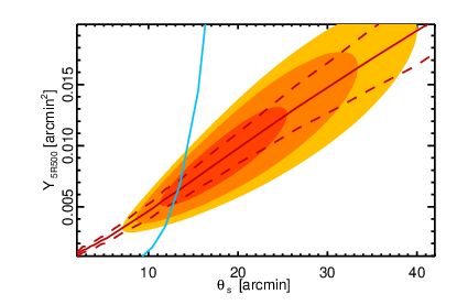
We illustrate our method in Fig. 16. At any fixed value of , we study the probability distribution and derive the associated to the maximum probability, i.e. the ridge line of the contours (red continous line in Fig. 16). We also derive the limits enclosing a probability and use them to define a upper and lower degeneracy curve (dashed lines). From the intersection of these three curves with the expected function (cyan line), we derive the estimate and its errors, by converting to and then applying the scaling relation prior at the redshift of the counterpart.
can be viewed as the hydrostatic mass expected for a cluster consistent with the assumed scaling relation, at a given redshift and given the Planck() posterior information. We find that this measure agrees with external X-ray and optical data with low scatter (see Sect. 7). For each measurement, the corresponding from the scaling relation prior can be calculated by applying the relation.
We underline that the errors bars calculated from this method consider only the statistical uncertainties in the contours, not the uncertainties on the pressure profile nor the errors and scatter in the scaling relation, and should thus be considered a lower limit to the real uncertainties on the mass.
We used the masses for the confirmation of candidate counterparts (see Sect. 7) and we provide them, along with their errors, in the PSZ2 catalogue for all detections with confirmed redshift. We compared them with the masses provided in PSZ1 for the detections where the associated counterpart (and thus the redshift value) has not changed in the new release (see Appendix B). We find very good agreement between the two values which are consistent within the error bars over the whole mass range.
In the individual catalogues, we provide for all entries an array of masses as a function of redshift (), which we obtained by intersecting the degeneracy curves with the expected function for different redshift values, from to . The aim of this function is to provide a useful tool for counterpart searches: once a candidate counterpart is identified, it is sufficient to interpolate the curve at the counterpart redshift to estimate its mass.
6 Consistency with the PSZ1
| A | ||||
|---|---|---|---|---|
| PSZ2 | PSZ1 |
The extra data available in the construction of the PSZ2 improves the detection S/N and reduces statistical errors in the parameter and location estimates. Here we assess the consistency between the two catalogues, given the matching scheme discussed in Sect. 7.1.
6.1 Signal-to-noise

We fit the relation between S/N for common PSZ1 and PSZ2 using the the approach and model discussed in Sect. 3.4. For the PSZ1 and PSZ2, the likelihoods for and have a strong covariance, as more than half of the PSZ2 observations were used in the construction of the PSZ1. We therefore assign a covariance of between the two S/N estimates, as is appropriate for Gaussian errors sharing 53% of the data. As the errors are not truly Gaussian, we allow for an intrinsic scatter between the S/N estimates to encapsulate any un-modelled component of the S/N fluctuation.
The consistency of the S/N estimates between the PSZ1 and PSZ2 are shown in Fig. 17 and the best fitting model in is shown in Table 3. Detections with PSZ2 are affected by changes in the MMF3 S/N definition. For the PSZ1, the empirical standard deviation of the filtered patches was used to define the S/N in this regime, while the theoretical standard deviation of Melin et al. (2006b) was used for lower S/N. MMF3 now uses the theoretical standard deviation for all S/N, consistent with the ESZ and the definitions in the other detection codes. For this reason, the best fit model ignores detections at in either catalogue. The MMF3 S/N show a flat improvement relative to the ESZ S/N (which was produced solely by MMF3), consistent with the reduced noise in the maps.
If the Compton-Y errors are entirely Gaussian in their behaviour, we should expect the S/N to increase by 37% between the PSZ1 and PSZ2, ie: . This is consistent within with the fit, which describes the S/N behaviour well to S/N.
6.2 Position estimation


The distribution of angular separations between the PSZ2 and PSZ1 position estimates is shown in Fig. 18. Of the common detections, 80% of the PSZ2 positions lie within one Planck map pixel width, 1.7 arcmin, of the PSZ1 position. MMF3 does not allow for sub-pixel positioning, so if the MMF3 position was used for the union in both the PSZ1 or PSZ2, the angular separation will be a multiple of the pixel width. This is evident in the cumulative distribution of angular separations as discontinuities at 0, 1 and pixel widths.
We also compare the position discrepancy between the SZ detection and the X-ray centres from the MCXC (Piffaretti et al. 2011).The bottom panel of Fig. 18 shows the distributions of these angular separations for the PSZ2 and PSZ1. The distributions are calculated from the full MCXC match for each catalogue: the PSZ2 includes 124 new detections. The PSZ2 position estimates are clearly closer to the X-ray centres than the PSZ1: for the PSZ1, the 67% error radius is 1.85 arcmin, while for the PSZ2 this reduces to 1.6 arcmin.
6.3 Missing PSZ1 detections
The PSZ1 produced 1227 union detections. While the numbers of detections has increased by 35% in the PSZ2 to 1653, the number of common detections is 936: 291 (23.7%) of the PSZ1 detections disappear. The high-purity intersection sample loses 44 detections, of which 20 are lost entirely, and 24 drop out of the intersection after one or two codes failed to detect them. In this section, we discuss these missing detections. Table 12 details each of the missing detections and provides an explanation for why each is missing.
The first type of missing detection are those that fall under the new survey mask, due to the increase in the number of point sources being masked. The masked areas sare pre-processed with harmonic infilling to prevent spurious detections induced by Fourier ringing. The increase of the mask area is driven by S/N improvements for IR sources in the high frequency channels. While the increase in the masked area is small (0.1% of the sky), the correlation between IR point sources and galaxy clusters leads to a larger percentage of detections being masked. In the PSZ1, these detections were contaminated by point source emission, but the emission was just beneath the point source masking threshold. 21 PSZ1 union detections fall behind the new mask. Of these, three were confirmed clusters, none received the highest validation quality flag of 1 (denoting probable clusters) in the PSZ1 validation process44 4 The PSZ1 validation process produced three quality flags for unconfirmed clusters. These were based on a combination of SZ signal quality, X-ray signal in the RASS maps and IR signal in the WISE maps. Class 1 candidates satisfied good quality in all three measures and were high reliability candidates. Class 2 satisfied at least one measure with good quality, while class 3 failed all three measures and so were considered probably spurious., four received the intermediate validation quality flag 2, and 14 received the lowest validation quality flag of 3, denoting probable spurious.
The second type of missing detection is one which has a matching detection in the full-mission data, but where the detection was rejected either by the infra-red spurious cuts or by PwS internal consistency cuts, both of which are discussed in Sect. 3.2. The IR cuts are responsible for cutting 33 unconfirmed PSZ1 detections, of which six were in the intersection sample. In the PSZ1 validation process, none of these received validation quality flag of 1, seven received quality flag 2 and 26 received quality flag 3. These were all detections. Five detections were lost because PwS was the only detecting code in the PSZ2 and they failed PwS consistency criteria: two of these were confirmed clusters.


The final type contains the majority (232) of the missing detections. These are low-significance detections close to the PSZ1 threshold that have downward-fluctuated with the full mission data and are now beneath the PSZ2 threshold. This occurs for some detections despite the fact that the S/N improves for most. The top panel of Fig. 19 shows the PSZ1 S/N distribution of the downward-fluctuated detections. These were weak detections: 87% were within of the detection threshold and 82% of them were single-code detections. While many of these may be spurious detections, 81 confirmed clusters have been lost. 61 of these were single-code detections and 70 of them were within of the threshold. Based on Planck data alone, these clusters were weak SZ detections and were likely to be Eddington biased above the threshold in the PSZ1. We have estimated the S/N for these lost PSZ1 detections in the full-mission maps using PwS in a non-blind analysis at the PSZ1 positions. Fig. 20 shows the distribution of these non-blind S/N: for most an apparently significant signal still exists in the maps, but it is now too weak to exceed the detection threshold, typically lying between . The non-blind S/N for this category is shown per detection in Table 12. Two detections have a non-blind S/N above the selection threshold. For these detections, the noise level for the non-blind analysis (centred on the PSZ1 location) was lower than for any of the patches in the mosaic used for the cluster detection.
To verify that this sample of missing detections is consistent with the change in data, we simulated the transition from the PSZ1 to the PSZ2 using FFP8 half-mission noise realisations to approximate the nominal mission: this produces a pair of data-sets with appropriately correlated noise characteristics. A common sample of clusters and point sources were injected into the simulations and the full pipeline was applied to construct catalogues from both simulated datasets. The simulations produced a total loss of 353 detections, of which 24 were lost due to the expansion of the point source mask, ten were lost due to changes to the PwS spurious rejection criteria, and 319 were lost due to downward fluctuation of the S/N beneath the detection threshold.
The S/N distribution of the latter group is shown in the bottom panel of Fig. 19. 75% lie within of the detection threshold and 85% were single-code detections. While this group was primarily composed of 230 spurious detections, 89 injected clusters were lost. The loss of these injected clusters illustrates that, as a statistical process, cluster detection is dependent on the realisation of the noise in the filtered patch-maps and we should expect that substantial numbers of confirmed but weak cluster detections will be lost due to noise fluctuations.
These simulations over-estimate the loss-rate of nominal mission detections. This may be due in part to unsimulated changes in the sample selection applied to the real data. We were unable to simulate systematic changes in the IR spurious rejection that may, had they been incorporated, have resulted in some spurious detections from the nominal mission simulation being cut from the comparison.
6.4 Compton Y estimates
The Compton estimates from each code are compared to the PSZ1 estimates in Fig. 21. The estimates that we consider here are the mean estimates of the marginal posteriors, having marginalised over the scale radius .
The best fit relations between the PSZ2 and PSZ1 values for each code are shown in Table 4. These were fit using a similar procedure to the S/N estimates discussed in the previous section. We assume a log-linear relation between the estimates of the form
| (7) |
with a log-normal intrinsic scatter and arcmin2. We again assume a bivariate Gaussian likelihood for the estimates, with a correlation of 0.72.
Fig. 21 compares the estimates for each of the three detection codes. High S/N detections have more consistent estimates of . For MMF3, detections at S/N are significantly changed due to the changes in the treatment of these detections discussed in Appendix C. These points are excluded from the fit to the relation. The scatter on the high S/N estimates is determined by the robustness of the noise power spectrum estimation to small changes in the data. For PwS, the high S/N estimates have particularly low scatter, due to the robust nature of the noise estimation that accounts for Compton-Y ‘noise’ contributed by neighbouring clusters.
The low S/N detections show systematic deviations for each of the codes. For the MMFs, these are caused by the correction of PSZ1 Eddington bias in the PSZ2 data, which is visible in Fig. 21 as clouds of faint points where the estimate reduces in the PSZ2. The opposite is the case for PwS estimates, where the faint detections show upward deviation in the PSZ2. This is caused by a change in the priors: for the PSZ1, PwS used a power-law prior in , which was replaced in the PSZ2 with the uninformative flat prior, as this produced more robust estimates in the posterior validation process discussed in the previous section. We have confirmed that PwS behaves in the same way as the MMFs when uninformative priors are used for both PSZ1 and PSZ2 parameter estimates (see the bottom right panel of Fig. 21).


| A | ||||
|---|---|---|---|---|
| PSZ1 MMF1 | PSZ2 MMF1 | |||
| PSZ1 MMF3 | PSZ2 MMF3 | |||
| PSZ1 PwS | PSZ2 PwS |
To verify that the bias effects seen in Fig. 21 are within expectations, we extracted estimates from the half to full-mission transition simulations described in Sec. 6.3. We confirm the same behaviour in these simulations as in the real data: low S/N detections from the MMFs show a correction of Eddington bias in the full mission while PwS low S/N detections are affected by change from power-law to uninformative priors in the posterior estimation and are typically higher in the full mission.
7 Ancillary Information
7.1 Cross-match with PSZ1
We begin the search for counterparts by conducting a cross-match with the well-validated PSZ1. All matches within 5 arcmin of a PSZ1 detection are accepted as a true match. Both catalogues used this radius as the merging limit to define unique detections, both in the merge of Cartesian patch catalogues to form an all-sky catalogue and in the formation of the union). This step produced no multiple matches.
Several of our detections are clear matches with PSZ1 detections at higher radii than this, so we consider matches out to 10 arcmin, as is the case with the X-ray and optical counterpart searches described below. This step produced 18 potential matches, two of which were non-unique. We apply a further condition to accept these high-separation matches: that the PSZ2 S/N be greater than the PSZ1 S/N and be consistent with the S/N relation determined in Sect. 6.1. For the two non-unique matches, the nearer match was chosen both times and this match also better fit the S/N relation.
7.2 X-ray information
We use the Meta-Catalogue of X-ray detected Clusters of
galaxies (MCXC, Piffaretti et al. 2011) for the association of Planck SZ
candidates with known X-ray clusters, as was done in
Planck Collaboration
XXIX (2014). MCXC is based on the ROSAT All Sky
Survey and complemented with other serendipitous catalogues and with
the Einstein Medium Sensitivity Survey. It includes 1743
clusters distributed over the whole sky and provides coordinates,
redshifts and X-ray luminosity measured within ,
. The association of Planck SZ candidates with
MCXC clusters follows two steps: first a positional matching between
the catalogues then a verification of the association using the
relation (Pratt et al. 2009). In the first step,
we looked for possible counterparts of Planck SZ candidates in the
MCXC within a searching radius of 10 arcmin around the
Planck position. We found one counterpart for candidates and
multiple matches for another 16 objects. In the second step, we
verified our associations by looking at their position in the
plane (Fig. 22). For the
X-ray luminosity, we use the value provided in the
MCXC, while we calculate the mass from our own data, as described in
Sect. 5. In Fig. 22, we compare our
results with the expected relation
(Piffaretti et al. 2011): we consider as good associations those whose position
in the does not differ from the expected
one by more than twice the intrinsic scatter in the relation
( Pratt et al. 2009). Based on this criterion
we discarded the association with an MCXC cluster for two objects,
PSZ2 G and PSZ2 G,
both new PSZ2 detections.
We performed a further check of the candidate counterparts, by
studying the separation between the Planck and the MCXC
positions. Indeed, the relatively large search radius (10 arcmin) may
have led to spurious associations, which might have escaped our
selection on the relation. In
Fig. 23, we compare the separation between the Planck and
the MCXC positions with two relevant angular scales: the positional
uncertainty of the Planck detections (
confidence level, provided in the catalogue) and the cluster size as
quantified by 55
5
We calculated
from the mass proxy , using the redshift of the MCXC
counterpart.. Ideally, one would keep as good counterparts those
systems where the angular separation is smaller than both
and (lower left quadrant in
Fig. 23) but this would lead to a large number of rejected
matches including many objects in the PSZ1. Therefore, we chose a
less conservative criterion: we excluded only those associations where
the separation is larger than both and
(upper right quadrant in Fig. 23). We
thus allow the separation to exceed if the MCXC
counterpart falls within the Planck accuracy (upper left quadrant)
and to exceed if it is smaller than the cluster expected
size (lower right quadrant). We noticed that the most deviant
clusters in the latter case (with ) are
associated with nearby clusters () with
arcmin, resolved by Planck. In this phase of the analysis, we thus
discarded the three associations to PSZ2 G, PSZ2
G, and PSZ2 G
in the upper right quadrant of Fig. 23: for these systems, the
separations between the Planck and MCXC are always
larger than 5 arcmin, which would correspond to a physical distance of
Mpc at the redshift of the MCXC objects (all at ).
We also used the position in the and in the separation plane (Fig. 23) to select the most likely counterparts for the objects where two or more MCXC clusters were found within our search radius of 10 arcmin. For seven out of 16 objects, one counterpart does not match the criteria described above and we are thus left with only one good counterpart. For six Planck detections, both MCXC counterparts fullfill our requirements. We thus rank them based on their distance from the scaling relation and their separation in terms of and , and select as most likely counterpart the one with smaller values for at least two out of three indicators. We provide details of the other possible counterparts in the Comments file. In two cases, the same MCXC cluster can be associated with two Planck detections and we used the procedure described above to select the most likely associations.
In the last step of our analysis, we checked our matching with MCXC with the matches made in the PSZ1 catalogue: in most cases the MCXC counterparts in the two catalogues coincide. We examined in detail the cases where, following our selection criteria, we would have broken the association with the MCXC counterpart which was chosen in PSZ1. This led to three restorations:
- •
PSZ2 G (PSZ1 index 842) association with RXCJ lies in the forbidden area in the separation plane. However, RXCJ (also known as A901) is a multi-component cluster (Bösch et al. 2013), and the PSZ2 position lies close to the position of one of the components. We thus decided to keep the association.
- •
PSZ2 G(PSZ1 index 1054) and PSZ2 G(PSZ1 index 1158) are both associated very low-redshift clusters (RXC J and RXC J, both ) which are marginal outliers in the L-M plane. However, our mass proxy estimate may be less reliable for local objects due to the large cluster extent and we thus decided to keep these associations.
7.2.1 Comparison to relation
It is interesting to note in Fig. 22 that most points lie below the expected scaling relations of Pratt et al. (2009), although well within the intrinsic scatter, meaning that clusters in our subsample are systematically under-luminous (by about 21%, or ) in X-rays at a given mass. We recall here that this subsample (intersection of PSZ2 with MCXC) is not representative and thus cannot be quantitatively compared with a well defined representative sample such as REXCESS, for which the was derived by Pratt et al. (2009). The systematic offset observed in Fig. 22 does not contradict the good agreement between X-ray predictions and Planck measurements found with a statistical approach in Planck Collaboration X (2011). It can be explained taking into account selection effects and the scatter in the scaling relation: when cutting in SZ S/N, clusters with a high SZ signal (and thus a high mass) for a given X-ray luminosity are preferentially selected. Another effect, which could also partly contribute to the offset in Fig. 22, is the presence of a cluster population with different X-ray properties in the PSZ2 sample which will be discussed in Sect. .


7.3 Optical information
We benefit from a wealth of publicly available data over the northern sky, principally thanks to the Sloan Digital Sky Survey (York et al. 2000, SDSS,) that covers most of the northern extragalactic sky with imaging in five optical bands (ugriz). A number of cluster catalogues have been extracted from these data using different finding algorithms (Koester et al. 2007; Hao et al. 2010; Wen et al. 2012). Among these, the redMaPPer catalogue (Rykoff et al. 2014), published since the PSZ1 release and containing many more clusters, has proven to be the most useful for identifying counterparts to Planck SZ sources. We also supplement redMaPPer with other optically information.
7.3.1 RedMAPPer
The redMaPPer algorithm detects clusters by looking for spatial over-densities of red-sequence galaxies. It provides accurate photometric redshift estimates for all sources, spectroscopic redshifts for the brightest central galaxy (BCG) when available, and richness estimates. We used the proprietary redMaPPer catalogue (v5.10) provided by the authors and containing over 400,000 objects.
In our procedure, detailed further in Bartlett et al. 2014 (in prep.), each Planck SZ source is first matched to a maximum of three redMaPPer clusters falling within a radius of 10 arcmin. They are subsequently ranked by richness and labeled first-, second-, and third-ranked matches. We then calculate the Planck mass proxy, , for each SZ source at the redshifts of its matched redMaPPer clusters. The best redMaPPer counterpart is then selected based on cuts in angular separation and richness. The angular cuts incorporate both the Planck positional uncertainty and the physical extent of the cluster estimated from the calculated .


These angular criteria alone would leave multiple possible counterparts in many cases, given the high surface density of redMaPPer clusters. Any ambiguity is efficiently reduced by the richness cut, which is based on the existence of a well-defined relation between richness, , and . The relation was established by Rozo et al. (2014) on the Planck 2013 SZ cluster catalogue and is expressed as
| (8) |
with , , and . The measured dispersion at given is .
In Fig. 24 we compare the distribution of the first, second-, and third-ranked redMaPPer matches in the plane to this scaling relation. The quantity is the deviation of measured richness from the expected mean. We see that the first-ranked matches (in red) display a prominent peak with . This reaffirms the existence of the scaling relation and motivates its use in defining the final redMaPPer counterparts for the PSZ2.


We define the best redMaPPer counterparts with the following cuts:
- 1.
OR ;
- 2.
;
- 3.
When more than one object remains a possible counterpart, we choose the highest ranked match.
The criteria on angular separation, , allow objects with centres either within Planck’s positional uncertainty or within the estimated size of the cluster (or both). The second criterion imposes the richness requirement based on the scaling relation. If there remain more than one possible counterpart satisfying these two criteria, then we choose the one with the largest richness. These latter cases, however, deserve closer examination, in particular for potential projection effects.
Fig. 25 shows the distribution of redMaPPer objects for Planck sources with single and double matches. The dashed lines delineate the angular cuts, while open circles identify those objects that also satisfy the richness cut. We see that the richness cut effectively eliminates objects that would be accepted on angular criteria alone. For the double matches, there are no good second-ranked redMaPPer counterparts because only the highest richness object satisfies the richness cut.
Table 5 summarizes the distribution of the 375 counterparts found with the above cuts. It is grouped into sets of columns for single-, double-, and triple-matched Planck objects. For each grouping, the total number of Planck sources is given in parentheses in the heading. The table entries list the number of matches in matrix format as follows: the element of a matrix gives the number of Planck sources with both - and -ranked redMaPPer counterparts; for example, six of the 438 triple matches have a good second-ranked counterpart only, while eight have both good first- and second-ranked counterparts.
|
|||||||||||||||||||||||||||||||||||||||||||||||||||
| One object with three possible good matches. |
7.3.2 Other optical information
We perform targeted searches for counterparts within the SDSS footprint for all Planck sources without good redMaPPer matches by applying the redMaPPer algorithm on a case-by-case basis. This yielded an additional 17 counterparts and associated redshifts.
We add optical confirmations and redshifts from several other sources. These include optical counterparts for PSZ1 clusters published recently from PanSTARRs (Liu et al. 2014) and from Planck collaboration optical follow-up observations (Planck Collaboration et al. 2014; Planck Collaboration Int. XXXV 2015). We also search for counterparts in the NED66 6 The NASA/IPAC Extragalactic Database (NED) is operated by the Jet Propulsion Laboratory, California Institute of Technology, under contract with the National Aeronautics and Space Administration. database, again removing any negated duplicate matches from the systematic searches. We compared the NED redshifts for PSZ2 matches to the redshifts from all the other ancillary catalogues we have studied. The NED redshifts have 88% agreement with these sources within . We therefore caution that NED redshifts should be considered the least reliable of our counterpart assignments. The NED associations are dominated by optical associations with Abell (Abell 1958) and Northern Optical Cluster Survey clusters (Gal et al. 2003).
Finally, we add four high-z counterparts confirmed using SDSS data and which are discussed in Appendix A.
7.4 IR information
At Planck detection positions, we have searched for galaxy overdensities in the AllWISE mid-infrared source catalogue (Cutri et al. 2013). The AllWISE source catalogue includes the combined cryogenic and NEOWISE (Mainzer et al. 2011) observations from the Wide-field Infrared Survey Explorer mission (WISE; Wright et al. 2010). The data cover the entire sky and we used the deepest bandpasses, the 3.4 (W1) and 4.6 (W2) channels. We predicted galaxy (W1-W2) colours from Bruzual & Charlot (2003) stellar population models, and searched for galaxy over-densities of the same colour in successive redshift ranges from z=0.3 to z=1.5 (e.g. Papovich et al. 2010; Mei et al. 2012; Mei et al. 2014; Stanford et al. 2014). At redshift , the contrast between red mid-infrared galaxies and the background is not efficient for galaxy cluster detection, so we searched only in the fields of Planck detections already validated at redshift , and detections not yet confirmed or with unknown redshift.
We estimated a significance of the over-densities by comparing the number of galaxies found in a region of co-moving diameter of 1 Mpc, with the background galaxies found in regions of the same area. To estimate the background density, we calculated for each redshift range both a local background for each candidate, in a region within 15 arcmin from the Planck detection, and a master background derived from the estimators for all the Planck fields. A substantial percentage of the Planck detections () are affected by artefacts from bright stars in the WISE data, which compromise meaningful assessment of the galaxy over-densities. The bulk of these are at low galactic latitude (). This means that we do not expect to reach a detection completeness of better of .
After visual inspection of all detections, we have flagged our detections in regions not affected by bright star artefacts with the following classification: 3 - Significant galaxy overdensity detected ; 2 - Probable galaxy overdensity; 1 - Possible galaxy overdensity; 0 - No significant galaxy overdensity. We also include these classifications for detections in regions affected by bright star artefacts: -1 Possible galaxy overdensity; -2 - No significant galaxy overdensity; -3 No assessment possible.
To test our classification, and evaluate our completeness and purity, we blindly apply our automated and visual inspection to 100 objects: 50 confirmed clusters and 50 random positions in the sky. We show the results of this validation test in Table 6: of the fields have images with bright star artefacts, including 17% which are class -3. In class 3 and 2, we obtain a and purity, respectively, for the validated clusters. Given the high purity of the class 3 detections, we classify these objects as confirmed infra-red clusters.
In Table 7, we show the number of WISE Planck detections in each class for the 935 Planck detections with or unknown redshift. A detailed study of the WISE detections will be published in a separate paper (Mei et al. 2015, in prep.). 73 new clusters have been confirmed (class 3 and not validated by other methods) by our WISE image analysis. A further 54 probable new clusters are identified (class 2 and unvalidated by other methods).
|
||||||||||||||||||||||||||||||||||||||||||
|
|||||||||||||||||||||||||||||||||||||||||||||||||||||||||
| aFor each WISE detection class, we show the total number of Planck detections and their percentage with respect to the 935 objects with known redshift or unknown redshift, the number of previously confirmed Planck clusters and the number of unconfirmed Planck detections. |
7.5 SZ information
We searched for counterparts of our Planck detections using
catalogues obtained with other SZ surveys, such as the South Pole
Telescope (SPT) and the Atacama Cosmology Telescope (ACT), and update
the list of SZ confirmations by direct follow-up with the Arc-minute
Micro-kelvin Interferometer (AMI).
7.5.1 SPT
For SPT, we refer to the recently released catalogue (Bleem et al. 2014),
extracted from the full 2500 deg2 SZ survey. It contains 677 SZ
detections, of which 516 have been confirmed as clusters, through
optical and near-IR observations. The catalogue contains the
photometric redshifts (spectroscopic when available) and mass estimate
of the confirmed clusters. More specifically, we chose to use the
“Fiducial Cosmology” Catalogue provided by the SPT collaboration, to
be consistent with the cosmological parameters used in the present
paper. We performed a two step matching process as described in
Sect. 7.2: a positional match within 10 arcmin, leading
to 89 single and five double matches, which we verified by comparing
our mass estimate with the one provided in the SPT catalogue. The mass
estimates are usually consistent at better than , except for
one detection, PSZ2 G, where they differ at
. We note, however, that the error bars on the
Planck mass reflect only the statistical error on the probability
contours and do not consider the uncertainties nor the intrinsic
scatter in the scaling relation used to break the
degeneracy. Moreover, as discussed also in the SPT case by
Bleem et al. (2014), the use of a fixed scaling relation and of a fiducial
cosmology results in an underestimation of the statistical and
systematic uncertainties in both datasets. Therefore, we decided to
keep the SPT counterparts for PSZ2 G, which is also
associated in the SPT catalogue to the same MCXC cluster (RXC
J) as in our matching. We checked the position of the
matches in the separation plane: none of the single matches have been
discarded in this way, while in four out of five multiple matches, one
of the counterparts was excluded following this criterion. In the
remaining match, two possible counterparts are allowed and we selected
as the most likely the one with a smaller mass difference and a
smaller separation in terms of .
We observe a systematic difference between the masses we derived from Planck data and those provided in the SPT catalogue. The mass is a derived quantity which requires scaling information to be assumed before it can be calculated from the SZ signal measured by either instrument. Comparison of the SZ observables is complicated by the different scales probed by each instrument: Planck is sensitive to the cluster outskirts while SPT is sensitive to the core regions. Any comparison necessarily requires model extrapolation, which is complicated further by the different pressure models used in the two measurements. A robust comparison will require a joint analysis of the data, which is beyond the scope of this paper.
7.5.2 ACT
For ACT, we use the catalogue published in Hasselfield et al. (2013), which contains both the most recent ACT detections and an update of the 23 Marriage et al. (2011) detections. 32 PSZ2 detections match with ACT clusters in a 10 arcmin radius. 28 have ACT UPP-based SZ masses consistent with Planck (less than deviation). Four have more than deviation: PSZ2 G053.44-36.25 (ACT-CLJ2135.1-0102) and PSZ2 G130.21-62.60 (ACT-CLJ0104.8+0002) are actually considered as good matches by our redMaPPer association, PSZ2 G262.27-35.38 (ACT-CLJ0516-5430) is also a good match for our MCXC association. The last one, PSZ2 G265.86-19.93 (ACT-CLJ0707-5522), is a good match in the PSZ1. We decided to leave blank the ACT field of the PSZ2 catalogue for these four clusters but, given the uncertainties on the mass determination and associated errors, we did not break the corresponding redMaPPer, MCXC and PSZ1 association.
7.5.3 AMI
Following the ongoing follow-up observations of the Planck cluster candidates, a total of clusters with S/N were observed with AMI. The detection significance is then characterised by calculating of the natural logarithm of the Bayes factor, ,
| (9) |
where and are the natural logarithm of the Bayesian evidence for model and respectively. Model accounts both for the cluster signal and the contribution from radio sources while only takes into account the radio source environment. Further details of the AMI observations, of the Bayesian methodology and of the modelling of interferometric SZ data, primordial CMB anisotropies, and resolved and unresolved radio point sources, as well as of the criteria used to categorise clusters are given in Perrott et al. (2014) and references therein.
In this context the detection significance for the clusters is described in Table 8. 132 of the 161 AMI-confirmed Planck clusters are included in the PSZ2.
|
7.6 Redshift compilation
We provide a single redshift estimate for each detection where at least one redshift is known for a matched counterpart. In many cases, we have multiple estimates per detection. This section discusses the compilation of redshift information and how redshifts are assigned in the final catalogue. Confirmation statistics and final assigned redshift numbers are summarised in Table 9.
Initial redshift estimates are taken from the PSZ1 catalogue redshift compilation, given the matching in Sect. 7.1. We include new follow-up results from the Planck collaboration (Planck Collaboration et al. 2014; Planck Collaboration Int. XXXV 2015), which include spectroscopic updates to PSZ1 photometric redshifts and new confirmations of PSZ1 detections. We also include external updates to PSZ1 counterpart redshifts from the NED and SIMBAD databases (Planck Collaboration XXXVI 2015).
After these steps, we cycle through priority levels in our systematic counterpart searches, in the following order of priority: MCXC, redMaPPer ACT and SPT. We compare the updated PSZ1 and MCXC redshifts with the redshifts from redMaPPer where available, and prioritise redMaPPer redshifts highest amongst available photometric redshifts. We test spectroscopic redshifts at for consistency within and of the redMaPPer photo-z. Any discrepancies are considered on an individual basis. In a small number of cases, we choose the redMaPPer redshift. We also reject a small number of counterpart assignments where that counterpart is a bad match in redMaPPer. These cases are discussed in Appendix B.
The common sample between the PSZ2 and each of the external samples is denoted in the catalogue. After the systematic searches, we assign any remaining unconfirmed clusters to database counterparts where available. If a PSZ1 match assigns to the same counterpart as one of the negated counterparts from the systematic searches, where the possible counterpart violated the consistency criteria, then the PSZ1 match is also negated.
|
8 Sample Properties
8.1 Mass and redshift properties
We discuss here the distribution of Planck SZ-selected clusters in the mass-redshift () plane, using the mass proxy derived with scaling relations as discussed in Sect. 7. For 1094 detections with known redshifts in the PSZ2 catalogue (Sect. 7), we show in Fig. 26 their position in the plane, compared with the expected completeness function of our survey (we show the 20%, 50% and 80% completeness levels). These curves indicate the points in the plane at which clusters have % chances to be detected. They were computed for the full survey area. The red points in Fig. 26 show the 298 new PSZ2 confirmed detections, with redshifts, that were not found in the previous version of the catalogue. The black points show the common PSZ1-PSZ2 detections.
We stress that the distribution in Fig. 26 cannot be considered as fully representative of the Planck SZ selection, since it reflects the biases due to the non-uniform knowledge of redshifts over the sky in the ancillary information we used (Sect. 7). For instance, we have an extensive redshift information in the sky area covered by the SDSS survey thanks to the redMaPPer catalogue (Rykoff et al. 2014) but not in the remaining part of the sky. The incomplete redshift information can also explain the rarity of new detections in the PSZ2 catalogue with respect to PSZ1 at high redshift: at we have 36 objects, but only four new PSZ2 detections. We note however that most of the PSZ1 clusters in this redshift range were not present in existing catalogues but they were confirmed as clusters and their redshift was measured thanks to the massive follow up campaign with optical and X-ray telescopes which was undertaken by the Planck Collaboration for PSZ1 candidates (Planck Collaboration XXIX 2014 and references therein) and which continued also after the 2013 release (Planck Collaboration et al. 2014; Planck Collaboration Int. XXXV 2015). Since a similar observational campaign has not yet been possible for new PSZ2 detections, we could not populate further the high-mass high-z part of the plane.
The new PSZ2 confirmed detections (red points in Fig. 26) are mostly low-mass objects close to the detection limit of the survey. The mean mass of confirmed clusters over the whole redshift range in the PSZ2 is , which is lower than in the PSZ1 (). The common sample of 795 objects contains the higher mass clusters detected by both surveys, with mean mass . This is expected, since the common sample contains none of the new low-mass PSZ2 detections and none of the missing low S/N PSZ1 detections, discussed in Sect. 6.3, which were likely to have been low mass.
This is also shown in Fig. 27, where we compare the mass distribution of the confirmed clusters in the PSZ2, the PSZ1 and their common sample, for several redshift bins. The median mass and the first and third quantiles are always lower for the PSZ2 than for the PSZ1 and the common sample, showing that we are significantly expanding the sample towards lower masses.
Fig. 26 also shows a comparison of the SZ selected samples from the Planck, ACT and SPT surveys. Planck tends to detect the rarest high-mass clusters observed at high-redshift in these partial-sky surveys and provides a complementary clean SZ selection at lower redshifts, where the Planck frequency range provides sufficient information to disentangle the SZ signal of large clusters from the background.


8.2 X-ray underluminous clusters
The presence of a bright cool-core, characterised by a peaked surface brightness profile, has been shown to bias X-ray flux selected cluster samples in favour of peaked, relaxed objects with respect to morphologically disturbed systems (Eckert et al. 2011). In contrast, SZ selected samples have produced more disturbed systems than expected, with SZ discovered clusters typically lying on the lower end of the mass-luminosity relation (Planck Collaboration IX 2011). There has also been much interest in the possible existence of severely X-ray under-luminous clusters, with several authors identifying potential systems (eg: Bower et al. 1997; Popesso et al. 2007; Dietrich et al. 2009; Trejo-Alonso et al. 2014 and references therein) and suggesting a model where these clusters are dynamically young objects, still undergoing accretion and mergers and yet to reach equilibrium. An alternative suggestion is that line-of-sight structures may bias mass and richness estimates high relative to the X-ray luminosity (Bower et al. 1997; Giles et al. 2015).
However, the reported under-luminosity of these objects is disputed. Andreon & Moretti (2011) note that the under-luminosity is often claimed relative to biased scaling relations, and that the significance of the under-luminosity is amplified due to underestimation of the true scatter in the relation.
In the SDSS area, the majority of Planck detections possess counterparts in the redMaPPer catalogue, with redshifts and optical richness estimates. We construct a test sample from the Planck-redMaPPer intersection at low redshift, . This sample of 148 clusters can be expected to be detectable in the ROSAT maps. While redMaPPer is not complete for the Planck mass ranges at these redshifts, it allows us to construct a sample that is independent of any X-ray selection effects and therefore well-suited for finding under-luminous clusters, as any biases in selection will affect both normal and under-luminous X-ray cluster alike.
For each of these clusters, we calculate the X-ray count-rate using a growth-curve analysis on the ROSAT keV band maps following Böhringer et al. (2000). We derived the count-rate and its upper and lower limit from the growth curve at , which we calculated from the Planck mass proxy. We then converted the RASS count rates into flux in the keV energy range, using an absorbed thermal model, where we used the galactic absorption at the Planck position, the redshift of the redMaPPer counterpart and the temperature derived from the mass proxy through the M-T scaling relation by Arnaud et al. (2007). We then converted fluxes into luminosity in the keV channel. We found good agreement with the reported MCXC values of for those clusters also present in the MCXC.


We then searched for outlier clusters from the - and relations, using the calculated following Sect. 5.3. In both cases, we find the best-fit relation for our sample using the BCES algorithm. To exclude outliers from the fits, we clipped objects with orthogonal residual from the best-fit relations, where is the raw scatter around the relation derived from the median-absolute deviation. We then iterated the sigma-clipping process until converged.
The top panels of Fig. 28 show the best-fit relations and their scatters between and redMaPPer richness , and between and , for the test sample of 148 Planck-redMaPPer clusters. The bottom panels of Fig. 28 show the histograms of , normalised by .
The points highlighted with larger cyan circles denote clusters with more than 2.5 below the best-fit relation. These clusters are under-luminous in X-rays for their . However, their estimates are consistent with their optical richness and do not lie preferentially beneath the relation. The consistency of optical and SZ mass proxies suggest either that these clusters are under-luminous for their mass, or that both the and estimates are biased high.
One exception to this is PSZ2 G127.71-69.55, discrepant with both relations: at for and for . It is circled in red in Figure 28. This is the only cluster in the Planck-redMaPPer sample with a poor Q_NEURAL flag and is either a failed redMaPPer match (lying close to the matching threshold in the plane) or a cluster with a severely IR contaminated spectrum for which the Planck estimate is likely overestimated. We therefore remove this from the list of under-luminous candidates.
We expanded the search for under-luminous clusters across the whole sky, testing all clusters with against the mean relation determined above. This expanded the number of under-luminous candidates to 22. These objects warrant follow-up observations to determine their dynamical state and to search for line-of-sight structures that may bias high both the and optical richness. They are flagged in the COMMENT field of the catalogue. They should be of interest in understanding the systematic differences between SZ and X-ray selection.
9 Summary
|
The Planck satellite is unique in providing broad frequency coverage over the whole sky with good sensitivity to both the high frequency spectral increment and the low frequency decrement of the thermal SZ effect. In this paper, we have presented second Planck catalogue of SZ sources (PSZ2). This is based on data from the full 29 month mission and uses a methodology that refines the one used to produce the PSZ1 from 15.5 months of data. The catalogue is based on the union of results from three cluster detection codes (Planck Collaboration XXIX 2014). The PSZ2 contains 1653 cluster candidates distributed across 83.6% of the sky. The catalogue was validated using external X-ray, optical, SZ and near infra-red data, producing confirmation for 1203 candidates with 1094 redshifts. The catalogue contains 716 new detections including 366 confirmed clusters with newly identified SZ signal. 87 of our confirmed clusters are newly identified in this paper. We have found good consistency with the PSZ1 and re-detect 937 SZ sources from the PSZ1 sample of 1227. We have investigated the missed detections: the vast majority of these were low-significance PSZ1 detections whose S/N has fluctuated beneath the detection threshold. The majority of these are expected to be spurious detections.
The current status of our knowledge of counterparts for our detections at various frequencies is summarised in Table 10 and compared to the PSZ1. Our optical validation scheme is based on the newly released SDSS-based redMaPPer catalogue (Rozo & Rykoff 2014). This produced 374 high-quality matches where the counterparts are consistent with Planck mass and position information. We reject 188 possible matches where the mass or position information is inconsistent with the Planck information. This underlines the importance of consistency checks when matching with high density SDSS catalogues. Our X-ray and SZ counterpart searches implement similar consistency criteria leading to tight control over mismatches.
Central to the counterpart search process is the understanding of the Planck SZ parameter estimates. We have validated the Planck Compton-Y posteriors using detailed simulations that include an ensemble of hydro-dynamically simulated pressure profiles that vary from the pressure profile assumed by our extraction algorithms. Our estimates are robust to mis-matches in the pressure profile. When translating to , we have shown the importance of accurate prior information about radius to break the degeneracy and produce accurate and precise estimates from the Planck data. Our counterpart searches make extensive use of the Planck mass-proxy; this uses prior information about redshift and scaling relations to derive mass constraints which show low scatter with respect to external estimates. We provide this for all candidates with a redshift, and provide in the range for all other candidates. We expect this information to be useful in future comparisons with external data.
Central to any statistical use of a cluster sample is the survey selection function. We have estimated the catalogue completeness using Monte-Carlo source injection and we provide this as a product for the full survey and for various sub-samples as a function of selection S/N. We have validated the completeness through a comparison with external X-ray data and high resolution SZ data from SPT (Bleem et al. 2014), which spans the redshift range and angular sizes of the Planck data. We estimate the catalogue to be 83-87% pure, based on simulations of the Planck data and detection-by-detection quality assessment utilising machine learning. Higher reliability sub-samples can be constructed easily: the main contaminant is infra-red galactic emission and as such the reliability is a strong function of galactic latitude. Specifically, the cluster cosmology zone that covers 65% of the sky contains 1308 detections at % reliability, and full survey intersection catalogue (objects detected by all three codes) contains 827 detections at reliability.
Cosmology using the cluster counts is also dependent on external observational data to provide cluster redshifts. Planck Collaboration XXIV (2015) have produced cosmological constraints using samples drawn from the PSZ2, containing 493 candidates from the intersection sample and 439 drawn from the single-code MMF3 sample. Utilising larger samples from the PSZ2 requires further redshift information. We also expect the PSZ2 to contain many high-mass clusters at . So far only 36 have been identified, of which 21 were identified in targeted follow-up observations of PSZ1 candidates. For these reasons, the PSZ2 should motivate further follow-up observations. In particular, the catalogue contains 73 clusters confirmed by WISE infra-red data that currently have no redshift information but which are likely to be high-redshift.
Understanding the biases in cluster selection that affect samples defined at different wavelengths will be important for interpreting statistical results from existing surveys and those planned for the near future. Using a low-redshift overlap sample from PSZ2 and redMaPPer, we have identified a population of low-z clusters with ‘typical’ optical and SZ properties, but which are underluminous for their mass in ROSAT X-ray data. These clusters may be part of a population of dynamically disturbed clusters that are under-represented in X-ray selected surveys. These objects will be interesting targets for multi-wavelength follow-up to determine their dynamical state.
In the near future, Planck all-sky SZ data can be combined with observations of the large-scale structure by surveys such as PAN-STARRS, LOFAR, Euclid, LSST, and RSG/e-ROSITA. This will provide an unprecedented multi-wavelength view of the evolution of large-scale structure that will revolutionise our understanding of the physics governing this process.
Acknowledgements.
The Planck Collaboration acknowledges the support of: ESA; CNES and CNRS/INSU-IN2P3-INP (France); ASI, CNR, and INAF (Italy); NASA and DoE (USA); STFC and UKSA (UK); CSIC, MINECO, JA, and RES (Spain); Tekes, AoF, and CSC (Finland); DLR and MPG (Germany); CSA (Canada); DTU Space (Denmark); SER/SSO (Switzerland); RCN (Norway); SFI (Ireland); FCT/MCTES (Portugal); ERC and PRACE (EU). A description of the Planck Collaboration and a list of its members, indicating which technical or scientific activities they have been involved in, can be found at http://www.cosmos.esa.int/web/planck/planck-collaboration. We thank Ian McCarthy for providing images and profiles of simulated clusters from cosmo-OWLS. This research has made use of the NASA/IPAC Extragalactic Database (NED), which is operated by the Jet Propulsion Laboratory, California Institute of Technology, under contract with the National Aeronautics and Space Administration, and the SIMBAD database, operated at CDS, Strasbourg, France This research made use of data retrieved from SDSS-III. Funding for SDSS-III has been provided by the Alfred P. Sloan Foundation, the Participating Institutions, the National Science Foundation, and the U.S. Department of Energy Office of Science. The SDSS-III web site is http://www.sdss3.org/. This research has made use of data processed by the Centre d’Analyse de Donnes Etendues http://cade.irap.omp.eu/ and has made use of the HEALPix pixelisation software http://healpix.sourceforge.net (Górski et al. 2005). This work was performed using the Darwin Supercomputer of the University of Cambridge High Performance Computing Service (http://www.hpc.cam.ac.uk/), provided by Dell Inc. using Strategic Research Infrastructure Funding from the Higher Education Funding Council for England and funding from the Science and Technology Facilities Council.References
- Abell (1958) Abell, G. O., The Distribution of Rich Clusters of Galaxies. 1958, ApJS, 3, 211
- Aghanim et al. (2014) Aghanim, N., Hurier, G., Diego, J.-M., et al., The Good, the Bad and the Ugly: Statistical quality assessment of SZ detections. 2014, astro-ph/1409.6543, 1409.6543
- Allen et al. (2011) Allen, S. W., Evrard, A. E., & Mantz, A. B., Cosmological Parameters from Observations of Galaxy Clusters. 2011, ARA&A, 49, 409, 1103.4829
- Andreon & Moretti (2011) Andreon, S. & Moretti, A., Do X-ray dark or underluminous galaxy clusters exist? 2011, A&A, 536, A37, 1109.4031
- Arnaud et al. (2007) Arnaud, M., Pointecouteau, E., & Pratt, G. W., Calibration of the galaxy cluster M500-YX relation with XMM-Newton. 2007, A&A, 474, L37, 0709.1561
- Arnaud et al. (2010) Arnaud, M., Pratt, G. W., Piffaretti, R., et al., The universal galaxy cluster pressure profile from a representative sample of nearby systems (REXCESS) and the YSZ - M500 relation. 2010, A&A, 517, A92, 0910.1234
- Benson et al. (2013) Benson, B. A., de Haan, T., Dudley, J. P., et al., Cosmological Constraints from Sunyaev-Zel’dovich-selected Clusters with X-Ray Observations in the First 178 deg2 of the South Pole Telescope Survey. 2013, ApJ, 763, 147, 1112.5435
- Bleem et al. (2014) Bleem, L. E., Stalder, B., de Haan, T., et al., Galaxy Clusters Discovered via the Sunyaev-Zel’dovich Effect in the 2500-square-degree SPT-SZ survey. 2014, ArXiv e-prints, 1409.0850
- Böhringer et al. (2004) Böhringer, H., Schuecker, P., Guzzo, L., et al., The ROSAT-ESO Flux Limited X-ray (REFLEX) Galaxy cluster survey. V. The cluster catalogue. 2004, A&A, 425, 367, arXiv:astro-ph/0405546
- Böhringer et al. (2000) Böhringer, H., Voges, W., Huchra, J. P., et al., The Northern ROSAT All-Sky (NORAS) Galaxy Cluster Survey. I. X-Ray Properties of Clusters Detected as Extended X-Ray Sources. 2000, ApJS, 129, 435, astro-ph/0003219
- Borgani & Kravtsov (2009) Borgani, S. & Kravtsov, A., Cosmological simulations of galaxy clusters. 2009, ArXiv e-prints, 0906.4370
- Bösch et al. (2013) Bösch, B., Böhm, A., Wolf, C., et al., Tully-Fisher analysis of the multiple cluster system Abell 901/902. 2013, A&A, 554, A97, 1304.6186
- Bower et al. (1997) Bower, R. G., Castander, F. J., Ellis, R. S., Couch, W. J., & Boehringer, H., A dynamical study of optically selected distant clusters. 1997, MNRAS, 291, 353, astro-ph/9705099
- Bruzual & Charlot (2003) Bruzual, G. & Charlot, S., Stellar population synthesis at the resolution of 2003. 2003, MNRAS, 344, 1000, astro-ph/0309134
- Burenin et al. (2007) Burenin, R. A., Vikhlinin, A., Hornstrup, A., et al., The 400 Square Degree ROSAT PSPC Galaxy Cluster Survey: Catalog and Statistical Calibration. 2007, ApJS, 172, 561, arXiv:astro-ph/0610739
- Carlstrom et al. (2002) Carlstrom, J. E., Holder, G. P., & Reese, E. D., Cosmology with the Sunyaev-Zel’dovich Effect. 2002, ARA&A, 40, 643, arXiv:astro-ph/0208192
- Carvalho et al. (2009) Carvalho, P., Rocha, G., & Hobson, M. P., A fast Bayesian approach to discrete object detection in astronomical data sets - PowellSnakes I. 2009, MNRAS, 393, 681, 0802.3916
- Carvalho et al. (2012) Carvalho, P., Rocha, G., Hobson, M. P., & Lasenby, A., PowellSnakes II: a fast Bayesian approach to discrete object detection in multi-frequency astronomical data sets. 2012, MNRAS, 427, 1384, 1112.4886
- Chamballu et al. (2012) Chamballu, A., Bartlett, J. G., & Melin, J.-B., The Planck SZ Cluster Catalog: expected X-ray properties. 2012, A&A, 544, A40
- Chen et al. (2007) Chen, Y., Reiprich, T. H., Böhringer, H., Ikebe, Y., & Zhang, Y.-Y., Statistics of X-ray observables for the cooling-core and non-cooling core galaxy clusters. 2007, A&A, 466, 805, astro-ph/0702482
- Crawford et al. (1995) Crawford, C. S., Edge, A. C., Fabian, A. C., et al., Optical spectroscopy of the ROSAT X-ray brightest clusters - II. 1995, MNRAS, 274, 75
- Cutri et al. (2013) Cutri, R. M., Wright, E. L., Conrow, T., et al. 2013, Explanatory Supplement to the AllWISE Data Release Products, Tech. rep.
- da Silva et al. (2004) da Silva, A. C., Kay, S. T., Liddle, A. R., & Thomas, P. A., Hydrodynamical simulations of the Sunyaev-Zel’dovich effect: cluster scaling relations and X-ray properties. 2004, MNRAS, 348, 1401, arXiv:astro-ph/0308074
- Dietrich et al. (2009) Dietrich, J. P., Biviano, A., Popesso, P., et al., Weak lensing observations of potentially X-ray underluminous galaxy clusters. 2009, A&A, 499, 669, 0903.3599
- Ebeling et al. (1998) Ebeling, H., Edge, A. C., Bohringer, H., et al., The ROSAT Brightest Cluster Sample - I. The compilation of the sample and the cluster log N-log S distribution. 1998, MNRAS, 301, 881, arXiv:astro-ph/9812394
- Ebeling et al. (2010) Ebeling, H., Edge, A. C., Mantz, A., et al., The X-ray brightest clusters of galaxies from the Massive Cluster Survey. 2010, MNRAS, 407, 83, 1004.4683
- Eckert et al. (2011) Eckert, D., Molendi, S., & Paltani, S., The cool-core bias in X-ray galaxy cluster samples. I. Method and application to HIFLUGCS. 2011, A&A, 526, A79, 1011.3302
- Gal et al. (2003) Gal, R. R., de Carvalho, R. R., Lopes, P. A. A., et al., The Northern Sky Optical Cluster Survey. II. An Objective Cluster Catalog for 5800 Square Degrees. 2003, AJ, 125, 2064, astro-ph/0301274
- Giles et al. (2015) Giles, P. A., Maughan, B. J., Hamana, T., et al., The X-ray properties of weak-lensing-selected galaxy clusters. 2015, MNRAS, 447, 3044, 1402.4484
- Górski et al. (2005) Górski, K. M., Hivon, E., Banday, A. J., et al., HEALPix: A Framework for High-Resolution Discretization and Fast Analysis of Data Distributed on the Sphere. 2005, ApJ, 622, 759, arXiv:astro-ph/0409513
- Haehnelt & Tegmark (1996) Haehnelt, M. G. & Tegmark, M., Using the Kinematic Sunyaev-Zeldovich effect to determine the peculiar velocities of clusters of galaxies. 1996, MNRAS, 279, 545, astro-ph/9507077
- Hao et al. (2010) Hao, J., McKay, T. A., Koester, B. P., et al., A GMBCG GALAXY CLUSTER CATALOG OF 55,424 RICH CLUSTERS FROM SDSS DR7. 2010, The Astrophysical Journal Supplement Series, 191, 254
- Harrison et al. (2014) Harrison, D., Sutton, D., Carvalho, P., & Hobson, M., Validation of Bayesian posterior distributions using a multidimensional Kolmogorov–Smirnov test. 2014, ArXiv e-prints, astro-ph/1404.7735
- Hasselfield et al. (2013) Hasselfield, M., Hilton, M., Marriage, T. A., et al., The Atacama Cosmology Telescope: Sunyaev-Zel’dovich selected galaxy clusters at 148 GHz from three seasons of data. 2013, J. Cosmology Astropart. Phys., 7, 8, 1301.0816
- Herranz et al. (2002) Herranz, D., Sanz, J. L., Hobson, M. P., et al., Filtering techniques for the detection of Sunyaev-Zel’dovich clusters in multifrequency maps. 2002, MNRAS, 336, 1057, astro-ph/0203486
- Hoekstra et al. (2012) Hoekstra, H., Mahdavi, A., Babul, A., & Bildfell, C., The Canadian Cluster Comparison Project: weak lensing masses and SZ scaling relations. 2012, MNRAS, 427, 1298, 1208.0606
- Hogg et al. (2010) Hogg, D. W., Bovy, J., & Lang, D., Data analysis recipes: Fitting a model to data. 2010, ArXiv e-prints, 1008.4686
- Kay et al. (2012) Kay, S. T., Peel, M. W., Short, C. J., et al., Sunyaev-Zel’dovich clusters in Millennium gas simulations. 2012, MNRAS, 422, 1999, 1112.3769
- Koester et al. (2007) Koester, B. P., McKay, T. A., Annis, J., et al., A MaxBCG Catalog of 13,823 Galaxy Clusters from the Sloan Digital Sky Survey. 2007, ApJ, 660, 239, arXiv:astro-ph/0701265
- Kravtsov et al. (2006) Kravtsov, A. V., Vikhlinin, A., & Nagai, D., A New Robust Low-Scatter X-Ray Mass Indicator for Clusters of Galaxies. 2006, ApJ, 650, 128, arXiv:astro-ph/0603205
- Le Brun et al. (2014) Le Brun, A. M. C., McCarthy, I. G., Schaye, J., & Ponman, T. J., Towards a realistic population of simulated galaxy groups and clusters. 2014, MNRAS, 441, 1270, 1312.5462
- Liu et al. (2014) Liu, J., Hennig, C., Desai, S., et al., Optical Confirmation and Redshift Estimation of the Planck Cluster Candidates overlapping the Pan-STARRS Survey. 2014, ArXiv e-prints, 1407.6001
- Mahdavi et al. (2013) Mahdavi, A., Hoekstra, H., Babul, A., et al., Joint Analysis of Cluster Observations. II. Chandra/XMM-Newton X-Ray and Weak Lensing Scaling Relations for a Sample of 50 Rich Clusters of Galaxies. 2013, ApJ, 767, 116, 1210.3689
- Mainzer et al. (2011) Mainzer, A., Bauer, J., Grav, T., et al., Preliminary Results from NEOWISE: An Enhancement to the Wide-field Infrared Survey Explorer for Solar System Science. 2011, ApJ, 731, 53, 1102.1996
- Marriage et al. (2011) Marriage, T. A., Acquaviva, V., Ade, P. A. R., et al., The Atacama Cosmology Telescope: Sunyaev-Zel’dovich-Selected Galaxy Clusters at 148 GHz in the 2008 Survey. 2011, ApJ, 737, 61, 1010.1065
- Maughan (2007) Maughan, B. J., The LX-YX Relation: Using Galaxy Cluster X-Ray Luminosity as a Robust, Low-Scatter Mass Proxy. 2007, ApJ, 668, 772, astro-ph/0703504
- McCarthy et al. (2014) McCarthy, I. G., Le Brun, A. M. C., Schaye, J., & Holder, G. P., The thermal Sunyaev-Zel’dovich effect power spectrum in light of Planck. 2014, MNRAS, 440, 3645, 1312.5341
- Mehrtens et al. (2012) Mehrtens, N., Romer, A. K., Hilton, M., et al., The XMM Cluster Survey: optical analysis methodology and the first data release. 2012, MNRAS, 423, 1024, 1106.3056
- Mei et al. (2014) Mei, S., Scarlata, C., Pentericci, L., et al., Star-forming blue ETGs in two newly discovered galaxy overdensities in the HUDF at z=1.84 and 1.9: unveiling the progenitors of passive ETGs in cluster cores. 2014, ArXiv e-prints, 1403.7524
- Mei et al. (2012) Mei, S., Stanford, S. A., Holden, B. P., et al., Early-type Galaxies at z = 1.3. I. The Lynx Supercluster: Cluster and Groups at z = 1.3. Morphology and Color-Magnitude Relation. 2012, ApJ, 754, 141, 1205.1785
- Melin et al. (2006a) Melin, J., Bartlett, J. G., & Delabrouille, J., Catalog extraction in SZ cluster surveys: a matched filter approach. 2006a, A&A, 459, 341, arXiv:astro-ph/0602424
- Melin et al. (2006b) Melin, J., Bartlett, J. G., & Delabrouille, J., Catalog extraction in SZ cluster surveys: a matched filter approach. 2006b, A&A, 459, 341, arXiv:astro-ph/0602424
- Melin et al. (2012) Melin, J.-B., Aghanim, N., Bartelmann, M., et al., A comparison of algorithms for the construction of SZ cluster catalogues. 2012, A&A, 548, A51, 1210.1416
- Mitra et al. (2011) Mitra, S., Rocha, G., Górski, K. M., et al., Fast Pixel Space Convolution for Cosmic Microwave Background Surveys with Asymmetric Beams and Complex Scan Strategies: FEBeCoP. 2011, ApJS, 193, 5, 1005.1929
- Papovich et al. (2010) Papovich, C., Momcheva, I., Willmer, C. N. A., et al., A Spitzer-selected Galaxy Cluster at z = 1.62. 2010, ApJ, 716, 1503, 1002.3158
- Peebles (1980) Peebles, P. J. E. 1980, The large-scale structure of the universe, ed. Peebles, P. J. E. (Princeton University Press)
- Perrott et al. (2014) Perrott, Y. C., Olamaie, M., Rumsey, C., et al., Comparison of Sunyaev-Zel’dovich measurements from Planck and from the Arcminute Microkelvin Imager for 99 galaxy clusters. 2014, ArXiv e-prints, 1405.5013
- Piffaretti et al. (2011) Piffaretti, R., Arnaud, M., Pratt, G. W., Pointecouteau, E., & Melin, J.-B., The MCXC: a meta-catalogue of x-ray detected clusters of galaxies. 2011, A&A, 534, A109+, 1007.1916
- Planck Collaboration (2011) Planck Collaboration. 2011, The Explanatory Supplement to the Planck Early Release Compact Source Catalogue (ESA)
- Planck Collaboration et al. (2014) Planck Collaboration, Ade, P. A. R., Aghanim, N., et al., Planck intermediate results. XXVI. Optical identification and redshifts of Planck clusters with the RTT150 telescope. 2014, ArXiv e-prints, 1407.6663
- Planck Collaboration IX (2011) Planck Collaboration IX, Planck early results. IX. XMM-Newton follow-up validation programme of Planck cluster candidates. 2011, A&A, 536, A9, 1101.2025
- Planck Collaboration X (2011) Planck Collaboration X, Planck early results. X. Statistical analysis of Sunyaev-Zeldovich scaling relations for X-ray galaxy clusters. 2011, A&A, 536, A10, 1101.2043
- Planck Collaboration XX (2014) Planck Collaboration XX, Planck 2013 results. XX. Cosmology from Sunyaev-Zeldovich cluster counts. 2014, A&A, 571, A20, 1303.5080
- Planck Collaboration XXIX (2014) Planck Collaboration XXIX, Planck 2013 results. XXIX. The Planck catalogue of Sunyaev-Zeldovich sources. 2014, A&A, 571, A29, 1303.5089
- Planck Collaboration XXXVI (2015) Planck Collaboration XXXVI, Planck 2013 results. XXIX. The Planck catalogue of Sunyaev-Zeldovich sources: Addendum. 2015, ArXiv e-prints, 1502.00543
- Planck Collaboration I (2015) Planck Collaboration I, Planck 2015 results. I. Overview of products and results. 2015, in preparation
- Planck Collaboration II (2015) Planck Collaboration II, Planck 2015 results. II. Low Frequency Instrument data processing. 2015, in preparation
- Planck Collaboration III (2015) Planck Collaboration III, Planck 2015 results. III. LFI systematic uncertainties. 2015, in preparation
- Planck Collaboration IV (2015) Planck Collaboration IV, Planck 2015 results. IV. LFI beams and window functions. 2015, in preparation
- Planck Collaboration V (2015) Planck Collaboration V, Planck 2015 results. V. LFI calibration. 2015, in preparation
- Planck Collaboration VI (2015) Planck Collaboration VI, Planck 2015 results. VI. LFI maps. 2015, in preparation
- Planck Collaboration VII (2015) Planck Collaboration VII, Planck 2015 results. VII. High Frequency Instrument data processing: Time-ordered information and beam processing. 2015, in preparation
- Planck Collaboration VIII (2015) Planck Collaboration VIII, Planck 2015 results. VIII. High Frequency Instrument data processing: Calibration and maps. 2015, in preparation
- Planck Collaboration IX (2015) Planck Collaboration IX, Planck 2015 results. IX. Diffuse component separation: CMB maps. 2015, in preparation
- Planck Collaboration X (2015) Planck Collaboration X, Planck 2015 results. X. Diffuse component separation: Foreground maps. 2015, in preparation
- Planck Collaboration XI (2015) Planck Collaboration XI, Planck 2015 results. XI. CMB power spectra, likelihood, and consistency of cosmological parameters. 2015, in preparation
- Planck Collaboration XII (2015) Planck Collaboration XII, Planck 2015 results. XII. Simulations. 2015, in preparation
- Planck Collaboration XIII (2015) Planck Collaboration XIII, Planck 2015 results. XIII. Cosmological parameters. 2015, in preparation
- Planck Collaboration XIV (2015) Planck Collaboration XIV, Planck 2015 results. XIV. Dark energy and modified gravity. 2015, in preparation
- Planck Collaboration XV (2015) Planck Collaboration XV, Planck 2015 results. XV. Gravitational lensing. 2015, in preparation
- Planck Collaboration XVI (2015) Planck Collaboration XVI, Planck 2015 results. XVI. Isotropy and statistics of the CMB. 2015, in preparation
- Planck Collaboration XVII (2015) Planck Collaboration XVII, Planck 2015 results. I. XVII. Constraints on primordial non-Gaussianity. 2015, in preparation
- Planck Collaboration XVIII (2015) Planck Collaboration XVIII, Planck 2015 results. XVIII. Background geometry and topology of the Universe. 2015, in preparation
- Planck Collaboration XIX (2015) Planck Collaboration XIX, Planck 2015 results. XIX. Constraints on primordial magnetic fields. 2015, in preparation
- Planck Collaboration XX (2015) Planck Collaboration XX, Planck 2015 results. XX. Constraints on inflation. 2015, in preparation
- Planck Collaboration XXI (2015) Planck Collaboration XXI, Planck 2015 results. XXI. The integrated Sachs-Wolfe effect. 2015, in preparation
- Planck Collaboration XXII (2015) Planck Collaboration XXII, Planck 2015 results. XXII. A map of the thermal Sunyaev-Zeldovich effect. 2015, in preparation
- Planck Collaboration XXIII (2015) Planck Collaboration XXIII, Planck 2015 results. XXIII. Thermal Sunyaev-Zeldovich effect–cosmic infrared background correlation. 2015, in preparation
- Planck Collaboration XXIV (2015) Planck Collaboration XXIV, Planck 2015 results. XXIV. Cosmology from Sunyaev-Zeldovich cluster counts. 2015, in preparation
- Planck Collaboration XXV (2015) Planck Collaboration XXV, Planck 2015 results. XXV. Diffuse, low-frequency Galactic foregrounds. 2015, in preparation
- Planck Collaboration XXVI (2015) Planck Collaboration XXVI, Planck 2015 results. XXVI. The Second Planck Catalogue of Compact Sources. 2015, in preparation
- Planck Collaboration XXVII (2015) Planck Collaboration XXVII, Planck 2015 results. XXVII. The Second Planck Catalogue of Sunyaev-Zeldovich Sources. 2015, in preparation
- Planck Collaboration XXVIII (2015) Planck Collaboration XXVIII, Planck 2015 results. XXVIII. The Planck Catalogue of Cold Clumps. 2015, in preparation
- Planck Collaboration Int. III (2013) Planck Collaboration Int. III, Planck intermediate results. III. The relation between galaxy cluster mass and Sunyaev-Zeldovich signal. 2013, A&A, 550, A129, 1204.2743
- Planck Collaboration Int. V (2013) Planck Collaboration Int. V, Planck intermediate results. V. Pressure profiles of galaxy clusters from the Sunyaev-Zeldovich effect. 2013, A&A, 550, A131, 1207.4061
- Planck Collaboration Int. XXXV (2015) Planck Collaboration Int. XXXV, Planck intermediate results. XXXV. Optical identification and redshifts of Planck SZ sources with telescopes in the Canary Islands Observatories. 2015
- Popesso et al. (2007) Popesso, P., Biviano, A., Böhringer, H., & Romaniello, M., RASS-SDSS galaxy cluster survey. V. The X-ray-underluminous Abell clusters. 2007, A&A, 461, 397, astro-ph/0606191
- Pratt et al. (2009) Pratt, G. W., Croston, J. H., Arnaud, M., & Böhringer, H., Galaxy cluster X-ray luminosity scaling relations from a representative local sample (REXCESS). 2009, A&A, 498, 361, 0809.3784
- Reichardt et al. (2013) Reichardt, C. L., Stalder, B., Bleem, L. E., et al., Galaxy Clusters Discovered via the Sunyaev-Zel’dovich Effect in the First 720 Square Degrees of the South Pole Telescope Survey. 2013, ApJ, 763, 127, 1203.5775
- Reiprich & Böhringer (2002) Reiprich, T. H. & Böhringer, H., The Mass Function of an X-Ray Flux-limited Sample of Galaxy Clusters. 2002, ApJ, 567, 716, arXiv:astro-ph/0111285
- Rodriguez-Gonzalvez et al. (2015) Rodriguez-Gonzalvez, C., Chary, R. R., Feroz, F., et al., CARMA observations of massive Planck-discovered cluster candidates at associated with WISE overdensities: breaking the size-flux degeneracy. 2015, in prep., in prep.
- Rozo & Rykoff (2014) Rozo, E. & Rykoff, E. S., redMaPPer II: X-Ray and SZ Performance Benchmarks for the SDSS Catalog. 2014, ApJ, 783, 80, 1303.3373
- Rozo et al. (2014) Rozo, E., Rykoff, E. S., Bartlett, J. G., & Melin, J. B., redMaPPer III: A Detailed Comparison of the Planck 2013 and SDSS DR8 RedMaPPer Cluster Catalogs. 2014, ArXiv e-prints, 1401.7716
- Rozo et al. (2010) Rozo, E., Wechsler, R. H., Rykoff, E. S., et al., Cosmological Constraints from the Sloan Digital Sky Survey maxBCG Cluster Catalog. 2010, ApJ, 708, 645, 0902.3702
- Rykoff et al. (2014) Rykoff, E. S., Rozo, E., Busha, M. T., et al., redMaPPer. I. Algorithm and SDSS DR8 Catalog. 2014, ApJ, 785, 104, 1303.3562
- Schaye et al. (2010) Schaye, J., Dalla Vecchia, C., Booth, C. M., et al., The physics driving the cosmic star formation history. 2010, MNRAS, 402, 1536, 0909.5196
- Schuecker et al. (2003) Schuecker, P., Böhringer, H., Collins, C. A., & Guzzo, L., The REFLEX galaxy cluster survey. VII. Omegam and sigma8 from cluster abundance and large-scale clustering. 2003, A&A, 398, 867, arXiv:astro-ph/0208251
- Sifón et al. (2013) Sifón, C., Menanteau, F., Hasselfield, M., et al., The Atacama Cosmology Telescope: Dynamical Masses and Scaling Relations for a Sample of Massive Sunyaev-Zel’dovich Effect Selected Galaxy Clusters. 2013, ApJ, 772, 25, 1201.0991
- Stanford et al. (2014) Stanford, S. A., Gonzalez, A. H., Brodwin, M., et al., The Massive and Distant Clusters of WISE Survey. II. Initial Spectroscopic Confirmation of z ˜ 1 Galaxy Clusters Selected from 10,000 deg2. 2014, ApJS, 213, 25, 1403.3361
- Staniszewski et al. (2009) Staniszewski, Z., Ade, P. A. R., Aird, K. A., et al., Galaxy Clusters Discovered with a Sunyaev-Zel’dovich Effect Survey. 2009, ApJ, 701, 32, 0810.1578
- Struble & Rood (1991) Struble, M. F. & Rood, H. J., A compilation of redshifts and velocity dispersions for Abell clusters (epoch 1991.2). 1991, ApJS, 77, 363
- Struble & Rood (1999) Struble, M. F. & Rood, H. J., A Compilation of Redshifts and Velocity Dispersions for ACO Clusters. 1999, ApJS, 125, 35
- Sunyaev & Zeldovich (1980) Sunyaev, R. A. & Zeldovich, I. B., Microwave background radiation as a probe of the contemporary structure and history of the universe. 1980, ARA&A, 18, 537
- Sunyaev & Zeldovich (1970) Sunyaev, R. A. & Zeldovich, Y. B., The Spectrum of Primordial Radiation, its Distortions and their Significance. 1970, Comments on Astrophysics and Space Physics, 2, 66
- Szabo et al. (2011) Szabo, T., Pierpaoli, E., Dong, F., Pipino, A., & Gunn, J., An Optical Catalog of Galaxy Clusters Obtained from an Adaptive Matched Filter Finder Applied to Sloan Digital Sky Survey Data Release 6. 2011, ApJ, 736, 21, 1011.0249
- Tinker et al. (2008) Tinker, J., Kravtsov, A. V., Klypin, A., et al., Toward a Halo Mass Function for Precision Cosmology: The Limits of Universality. 2008, ApJ, 688, 709, 0803.2706
- Trejo-Alonso et al. (2014) Trejo-Alonso, J. J., Caretta, C. A., Laganá, T. F., et al., Red sequence of Abell X-ray underluminous clusters. 2014, MNRAS, 441, 776, 1403.6437
- Vikhlinin et al. (2009a) Vikhlinin, A., Burenin, R. A., Ebeling, H., et al., Chandra Cluster Cosmology Project. II. Samples and X-Ray Data Reduction. 2009a, ApJ, 692, 1033, 0805.2207
- Vikhlinin et al. (2009b) Vikhlinin, A., Kravtsov, A. V., Burenin, R. A., et al., Chandra Cluster Cosmology Project III: Cosmological Parameter Constraints. 2009b, ApJ, 692, 1060, 0812.2720
- Wen et al. (2009) Wen, Z. L., Han, J. L., & Liu, F. S., Galaxy Clusters Identified from the SDSS DR6 and Their Properties. 2009, ApJS, 183, 197, 0906.0803
- Wen et al. (2012) Wen, Z. L., Han, J. L., & Liu, F. S., A Catalog of 132,684 Clusters of Galaxies Identified from Sloan Digital Sky Survey III. 2012, ApJS, 199, 34, 1202.6424
- Wright et al. (2010) Wright, E. L., Eisenhardt, P. R. M., Mainzer, A. K., et al., The Wide-field Infrared Survey Explorer (WISE): Mission Description and Initial On-orbit Performance. 2010, AJ, 140, 1868, 1008.0031
- York et al. (2000) York, D. G., Adelman, J., Anderson, Jr., J. E., et al., The Sloan Digital Sky Survey: Technical Summary. 2000, AJ, 120, 1579, astro-ph/0006396
- Zu et al. (2014) Zu, Y., Weinberg, D. H., Rozo, E., et al., Cosmological constraints from the large-scale weak lensing of SDSS MaxBCG clusters. 2014, MNRAS, 439, 1628
Appendix A High-redshift SDSS confirmations
Table 11 gives optical information for four high-redshift confirmations found using a search in SDSS data around unmatched Planck detections.
We use a multi-wavelength approach to confirm the clusters. Each of these candidates possess coincident high-redshift optical over-densities in SDSS, firm infra-red confirmations from WISE, and significant emission in the ROSAT keV band. We estimate the X-ray luminosity from the ROSAT maps using growth-curve analysis, and confirm that the luminosity is consistent with the measured as discussed in Sect. 7.2.
One interesting case is PSZ2 G097.52+51.70, which appears to be a near line-of-sight projection with components at and , separated by arcmin. Both systems may contribute to the observed Planck signal. We have associated to the high-redshift cluster because it is significantly closer to the SZ centre ( arcmin vs. arcmin separation), and because it is coincident ( arcmin) with the ROSAT X-ray centre. The system shows less significant hard-band emission.
| NAME | ||||
|---|---|---|---|---|
| PSZ2 G076.18-47.30 | 343.1475 | 4.5381 | 0.666 | 3 |
| PSZ2 G087.39+50.92 | 231.6383 | 54.1520 | 0.748 | 1 |
| PSZ2 G089.39+69.36 | 208.4382 | 43.4843 | 0.68 | |
| PSZ2 G097.52+51.70 | 223.8374 | 58.8707 | 0.7 |
Appendix B Differences in PSZ1 and PSZ2 redshift assignments
The PSZ2 contains 782 clusters which had redshift estimates in the PSZ1. We assign the same redshift in all but 43 of these cases. In 25 of these cases, there is no significant difference, defined by or , between the estimates and we have updated PSZ1 photometric redshift from various sources to new estimates from redMaPPer or Planck follow-ups.
We have updated a further seven PSZ1 photometric redshifts with recent Planck ENO follow-up redshifts (Planck Collaboration Int. XXXV 2015) where the redshift has significantly changed. Of these, one was from the PSZ1 SDSS search, two were from PanSTARRs and four were from earlier Planck photometric follow-ups. These updates are included in the 2015 update of the PSZ1 redshift compilation (Planck Collaboration XXXVI 2015).
We discuss the remaining 11 significant differences below:
- •
PSZ2 G020.66+37.99 (PSZ1 INDEX 51):
Rozo et al. (2014) discuss this cluster in depth. RedMAPPer finds two overlapping clusters, and . The PSZ1 redshift from WFI Planck follow-up is likely to be biased by members from the less rich and more distant system. For the PSZ2, we choose the higher richness match and quote the . The 2015 update to the PSZ1 adopts this change. - •
PSZ2 G066.68+68.44 (PSZ1 INDEX 222):
This is an ambiguous system. The PSZ1 used from NORAS (Böhringer et al. 2000). For the PSZ2 we have quoted from redMaPPer which agrees with the estimate from BCS follow-up (Struble & Rood 1999; Crawford et al. 1995) and the SDSS BCG estimate . The decision between these two ROSAT follow-up spectroscopic redshifts rests on the redMaPPer information, which identifies a rich system at . - •
PSZ2 G087.39+50.92 (PSZ1 INDEX 299):
The PSZ2 position has moved closer to a clear high-redshift SDSS cluster at at separation , and away from the PSZ1 SDSS match which is now at . There is also clear ROSAT keV X-ray emission at the high-z location, whose strength is consistent with the SZ emission, while there is no significant emission at the PSZ1 SDSS match location. - •
PSZ2 G090.66-52.34 (PSZ1 INDEX 308):
The PSZ1 redshift came from a single galaxy spectrum (Struble & Rood 1999). redMaPPer suggest this galaxy is likely to be in the foreground, with the rich cluster at slightly high redshift . We note however that the difference is small (10.2%). - •
PSZ2 G113.91-37.01 (PSZ1 INDEX 416):
We adopt the Rozo et al. (2014) update of the NORAS redshift, which replaced a group at with a rich cluster at separated by arcmin. - •
PSZ2 G121.13+49.64 (PSZ1 INDEX 443):
We note that this system is a probable projection. We adopt the correction of the redshift from (Rozo et al. 2014), noting that the richness of the component is consistent with the SZ signal, while the system matched in the PSZ1 is insufficiently rich. The 2015 update to the PSZ1 adopts this change. - •
PSZ2 G143.26+65.24 (PSZ1 INDEX 513):
The PSZ1 association with ACO 1430 is correct, but we update the redshift of from two members (Struble & Rood 1991) with from redMaPPer. The X-ray and optical images show an E-W elongation and two possible galaxy concentrations, possibly a projection. The high-redshift component has richness consistent with the SZ signal. The 2015 update to the PSZ1 adopts this change. - •
PSZ2 G151.19+48.27 (PSZ1 INDEX 537):
The PSZ1 association with A0959 is correct. NED lists two literature redshifts for this cluster: 0.289 (which we adopt) and 0.353 (adopted in the PSZ1). This object is bimodal in the optical and in the X-ray and is almost certainly a projection. redMaPPer suggests association with 0.289 component based on consistency of richness with the SZ signal. The 2015 update to the PSZ1 adopts this change. - •
PSZ2 G259.30+84.41 (PSZ1 INDEX 888):
We adopt the correction of Rozo et al. (2014) of the PSZ1 redshift from NSCS, instead matching to a clear and rich SDSS cluster within 1 arcmin of the Planck position at . The 2015 update to the PSZ1 adopts this change. - •
PSZ2 G310.81+83.91 (PSZ1 INDEX 1093):
The PSZ2 matched to an SDSS cluster at . redMaPPer finds this potential counterpart to be insufficiently rich to be detected by Planck at this redshift and there is no X-ray emission in ROSAT. The Planck detection may be spurious: there are point sources detected at 353 and 545GHz and the neural network quality assessment suggests a contaminated spectrum. We therefore break the association and leave the detection unconfirmed. - •
PSZ2 G318.62+58.55 (PSZ1 INDEX 1123):
We adopt the correction of Rozo et al. (2014) of the PSZ1 redshift . This associates to a different cluster at arcmin separation, with redMaPPer redshifts (), and richness .
Appendix C Modifications of the extraction algorithms since the PSZ1 release
C.1 MMF1
The MMF1 code used for the PSZ2 is the same as for the PSZ1 with the following changes:
- •
Positions estimates are now calculated with sub-pixel positioning using posteriors marginalised over all other parameters, rather than taking the pixel centre closest to the peak.
- •
Position error radius estimation has been debugged.
- •
The 2D contour grids for () expand dynamically if the 91% confidence region is not entirely contained within the grid. This expansion is not applied to S/N detections.
C.2 MMF3
For the PSZ2 release, we made three improvements on our MMF3 code:
- •
Bright clusters impact the estimation of background. For the PSZ1 we have adopted two different estimators of the MMF3 background depending on the S/N of the detections. If the S/N was below 20, the theoretical calculation was used (see Eq. 7 in Melin et al. (2006b)) while, for S/N greater than 20, we used the standard deviation of the filtered map. When the cluster signal is subdominant in the map the two estimators return the same result but they differ if the cluster is bright (typically with S/N above 20) due to the contamination of the background by the cluster itself. The choice of using two estimators has been made to make the MMF3 background estimate compatible with PwS and MMF1 for the PSZ1. We tested it against the QA after the 2013 release and found that it biases significantly MMF3 two dimensional (,) contours with respect to injected cluster size and flux at high S/N. We thus decided to come back to the theoretical calculation of the background across all the S/N range as in the earlier version of MMF3 used for the ESZ. This choice fixes the issue with high S/N cluster contours in the QA. But it increases the S/N value and shifts the (,) contours for MMF3 detections in the PSZ2 release with respect to PSZ1 for the detections with S/N above 20 more than the increase expected from the additional integration time. For the PSZ2 PwS now estimate the cross-channel covariance matrix under the ‘native’ prescription (see PwS section in this appendix). This improvement makes the background estimate compatible with the theoretical calculation from MMF3 and also gives unbiased estimates for the PwS two dimensional in the QA.
- •
MMF3 two dimensional (,) contours in the PSZ1 were tested against the QA after the 2013 release. This could not be done in early 2013 for lack of time. The contours were found to be wider than expected. The code has been corrected and new contours have been produced and included in the Planck Legacy Archive for the PSZ1. The PSZ2 relies on this new and fully tested estimate of the two dimensional contours.
- •
The MMF3 positional error for the PSZ1 was overestimated. The code has been corrected and tested against the QA. New estimates have been produced and included in the Planck Legacy Archive for the PSZ1. The PSZ2 uses the new estimate of the positional error.
C.3 PwS
The PwS code used for PSZ2 is similar to the one used for PSZ1, with two modifications:
- •
The cross-channel covariance matrix is now always estimated using iterative recalibration but is parameterised in order to produce a smoother estimate. Using the QA, we have shown that the new calibration only impacts the S/N estimate (%) keeping unchanged all other parameter estimates. The new S/N estimates are consistent with the other codes.
- •
For (,), we now adopt non-informative priors, formulated using Jeffrey’s method (Carvalho et al. 2012), instead of informative priors derived from a fiducial cosmology and mass function.
Appendix D Description of the delivered products
The data products comprise: (i) the main catalogue, which contains the characterised catalogue with ancillary information; (ii) individual algorithm catalogues produced by each of the codes prior to merging to create the main catalogue, which contain parameter posteriors per cluster; (iii) selection function files containing the completeness and survey masks for various sample definitions.
D.1 Main catalogue
The table contains the following columns:
| Column Name | Data Type | Units | Description |
|---|---|---|---|
| INDEX . | Integer(4) | … | Index of detection (see note 1) |
| NAME . | String | … | Name of detection (see note 2) |
| GLON . | Real(8) | degrees | Galactic longitude () |
| GLAT . | Real(8) | degrees | Galactic latitude () |
| RA . | Real(8) | degrees | Right ascension (J2000) |
| DEC . | Real(8) | degrees | Declination (J2000) |
| POS_ERR . | Real(4) | arcmin | Uncertainty in position (see note 3) |
| SNR . | Real(4) | … | S/N of detection |
| PIPELINE . | Integer(4) | … | Pipeline from which information is taken: the reference pipeline (see note 4) |
| PIPE_DET . | Integer(4) | … | Information on pipelines making detection (see note 4) |
| PCCS2 . | Boolean | … | Indicates whether detection matches with any in PCCS2 catalogues |
| PSZ . | Integer(4) | … | Index of matching detection in PSZ1, or -1 if a new detection |
| IR_FLAG . | Integer(1) | … | Flag denoting heavy IR contamination |
| Q_NEURAL . | Real(4) | … | Neural network quality flag (see note 5) |
| Y5R500 . | Real(4) | arcmin2 | Mean marginal as measured by the reference pipeline |
| Y5R500_ERR . | Real(4) | arcmin2 | Uncertainty on as measured by the reference pipeline |
| VALIDATION . | Integer(4) | … | External validation status (see note 6) |
| REDSHIFT_ID . | String | … | External identifier of cluster associated with redshift measurement (see note 7). |
| REDSHIFT . | Real(4) | … | Redshift of cluster (see note 7) |
| MSZ . | Real(4) | SZ mass proxy (see note 8) | |
| MSZ_ERR_UP . | Real(4) | Upper 1 SZ mass proxy confidence interval (see note 8) | |
| MSZ_ERR_LOW . | Real(4) | Lower 1 SZ mass proxy confidence interval (see note 8) | |
| MCXC . | String | … | ID of X-ray counterpart in the MCXC if one is present |
| REDMAPPER . | String | … | ID of optical counterpart in the redMaPPer catalogue if one is present |
| ACT . | String | … | ID of SZ counterpart in the ACT catalogues if one is present |
| SPT . | String | … | ID of SZ counterpart in the SPT catalogues if one is present |
| WISE_FLAG . | Integer(4) | … | Confirmation flag of WISE IR overdensity (see note 9) |
| AMI_EVIDENCE . | Real(4) | … | Bayesian evidence for AMI counterpart detection (see note 9) |
| COSMO . | Boolean | … | Indicates whether the cluster is in the cosmology sample |
| COMMENT . | String | … | Comments on this detection |
Notes:
- 1.
The index is determined by the order of the detections in the union catalogue. The matching entries in the individual catalogues have the same index to facilitate cross-referencing.
- 2.
The names are in the format PSZ2 Gxxx.xxyy.yy where xxx.xx is the Galactic longitude and yy.yy is the Galactic latitude of the detection, both in degrees. The coordinates are truncated towards zero, not rounded.
- 3.
The value given here is the 95% confidence interval of the distribution of radial displacement.
- 4.
The PIPELINE column defines the pipeline from which the values in the union catalogue are taken: 1 = MMF1; 2 = MMF3; 3 = PwS.
The PIPE_DET column is used to indicate which pipelines detect this object. The three least significant decimal digits are used to represent detection or non-detection by the pipelines. Order of the digits: hundreds = MMF1; tens = MMF3; units = PwS. If it is detected then the corresponding digit is set to 1, otherwise it is set to 0.
- 5.
The neural network quality flag is 1-, following the definitions in Aghanim et al. 2014. Values Q_NEURAL denote low-reliability detections.
- 6.
The VALIDATION column gives a summary of the external validation, encoding the most robust external identification: -1 = no known external counterpart; 10=ENO follow-up; 11= RTT follow-up; 12= PanSTARRs; 13= redMaPPer non-blind; 14= SDSS high-z; 15=AMI; 16= WISE; 20 = legacy identification from the PSZ1 2013 release; 21 = MCXC; 22= SPT; 23=ACT; 24= redMaPPer; 25= PSZ1 counterpart with redshift updated in (Planck Collaboration XXXVI 2015); 30= NED.
- 7.
The redshift source is the most robust external validation listed in the VALIDATION field.
- 8.
Definition of . The hydrostatic mass, , assuming the best-fit scaling relation of Arnaud et al. (2010) as a prior that cuts a plane through the parameter contours (see Sect. 5.3). The errors are 67% confidence statistical errors and based on the Planck measurement uncertainties only. Not included in the error estimates are the statistical errors on the scaling relation, the intrinsic scatter in the relation, or systematic errors in data selection for the scaling relation fit.
- 9.
WISE confirmation flag is assigned by visual inspection and defined to be one of , where -10 denotes no information and the other values are discussed in Section 7.4. Bayesian evidence for AMI counterpart defined in paper.
D.2 Individual algorithm catalogues
The table contains the following columns:
| Column Name | Data Type | Units | Description |
|---|---|---|---|
| INDEX . | Integer(4) | … | Index of detection (see note 1) |
| NAME . | String | … | Name of detection (see note 1) |
| GLON . | Real(8) | degrees | Galactic longitude () |
| GLAT . | Real(8) | degrees | Galactic latitude () |
| RA . | Real(8) | degrees | Right ascension (J2000) |
| DEC . | Real(8) | degrees | Declination (J2000) |
| POS_ERR . | Real(4) | arcmin | Uncertainty in position (see note 2) |
| SNR . | Real(4) | … | S/N of detection (see note 3) |
| TS_MIN . | Real(4) | arcmin | Minimum in second extension HDU (see note 4) |
| TS_MAX . | Real(4) | arcmin | Maximum in second extension HDU (see note 4) |
| Y_MIN . | Real(4) | arcmin2 | Minimum in second extension HDU (see note 4) |
| Y_MAX . | Real(4) | arcmin2 | Maximum in second extension HDU (see note 4) |
Notes:
- 1.
The index and name are taken from the union catalogue. The matching entries in the individual catalogues have the same index and name to facilitate cross-referencing.
- 2.
The value given here is the 95% confidence interval of the distribution of radial displacement.
- 3.
The SNR column contains the native signal-to-noise ratio determined by the detection pipeline.
- 4.
These entries define the limits of the grid used to evaluate the 2D probability distribution of and in the second extension HDU (see below).
Second extension HDU
The second extension HDU contains a three-dimensional image with the two-dimensional probability distribution in and for each cluster. The probability distributions are evaluated on a linear grid between the limits specified in the first extension HDU. The limits are determined independently for each detection. The dimensions of the 3D image are , where is the number of detections in the catalogue. The second dimension is and the first dimension is .
Third extension HDU
The third extension HDU contains a three-dimensional image with the observable information per cluster as a function of assumed redshift. The image dimensions are , where is the number of detections in the catalogue. The first dimension is the assumed redshift. The second dimension has size : the first element is the assumed redshift value for the fields. The second element is the lower 67% confidence bound, the third element is the estimate and the fourth element is the upper 67% confidence bound, all in units of . These errors are based on the Planck measurement uncertainties only. Not included in the error estimates are the statistical errors on the scaling relation, the intrinsic scatter in the relation, or systematic errors in data selection for the scaling relation fit.
D.3 Selection function file format
The selection function information is stored in FITS files. The filenames of the catalogues are of the form PSZ2-selection_Rx.xx.fits, where x.xx is the release number.
First extension HDU
The first extension HDU contains the survey region, denoted by an ring-ordered HEALPix map in GALACTIC coordinates. Pixels in the survey region have the value 1.0 while areas outside of the survey region have value 0.0.
Second extension HDU
The second extension HDU contains a three-dimensional image containing the survey completeness probability distribution for various thresholds. The information is stored in an image of size . The first dimension is , the second dimension is and the third dimension is the signal-to-noise threshold. The units are percent and lie in the range 0-100 and denote the detection probability of a cluster lying within the given - bin.
Third extension HDU
The second extension HDU contains the grid values for the completeness data cube held in the second extension. It has length 30 and spans the range arcmin2 in logarithmic steps.
Fourth extension HDU
The fourth extension HDU contains the grid values for the completeness data cube held in the second extension. It has length 32 and spans the range 0.9416-35.31 arcmin in logarithmic steps.
Fifth extension HDU
The fifth extension HDU contains the signal-to-noise threshold grid values for the completeness data cube held in the second extension. It has length 12 and contains thresholds at intervals of 0.5 from 4.5 to 10.0.
Appendix E Detail of missing PSZ1 detections
| Index | S/N | Pipeline | Pipe_det | Id_ext | Redshift | S/N (non-blind) | Type |
|---|---|---|---|---|---|---|---|
| 4. | 6.04 | 3 | 101 | … | … | … | 3 |
| 8 . | 4.92 | 1 | 100 | … | … | 0.34 | 1 |
| 9 . | 5.76 | 1 | 100 | … | … | … | 3 |
| 13 . | 4.52 | 1 | 100 | ZwCl 1454.5+0656 | 0.429 | 3.73 | 1 |
| 28 . | 4.70 | 2 | 10 | … | 0.46 | 3.54 | 1 |
| 30 . | 4.72 | 1 | 100 | … | … | 1.83 | 1 |
| 32 . | 4.54 | 1 | 100 | … | … | 1.65 | 1 |
| 34 . | 4.50 | 1 | 100 | … | … | 1.42 | 1 |
| 38 . | 4.65 | 1 | 100 | … | … | 2.48 | 1 |
| 40 . | 4.89 | 2 | 10 | … | … | 2.90 | 1 |
| 41 . | 4.81 | 2 | 10 | … | … | 2.90 | 1 |
| 43 . | 4.76 | 2 | 10 | … | … | 2.69 | 1 |
| 52 . | 5.71 | 2 | 10 | … | 0.39 | … | 4 |
| 58 . | 4.56 | 1 | 100 | … | … | 2.06 | 1 |
| 59 . | 4.63 | 1 | 100 | … | … | 3.27 | 1 |
| 60 . | 4.84 | 2 | 10 | RXC J1917.5-1315 | 0.177 | 3.11 | 1 |
| 61 . | 5.06 | 2 | 111 | … | 0.650893 | 2.91 | 1 |
| 62 . | 4.95 | 2 | 11 | ACO S 1010 | 0.28 | 4.02 | 1 |
| 66 . | 5.20 | 2 | 10 | … | … | 3.19 | 1 |
| 68 . | 4.67 | 3 | 1 | … | … | 3.45 | 1 |
| 77 . | 4.58 | 1 | 100 | RXC J1453.1+2153 | 0.1186 | 2.96 | 1 |
| 82 . | 4.98 | 2 | 10 | … | … | 2.84 | 1 |
| 83 . | 4.96 | 2 | 10 | … | … | 3.53 | 1 |
| 84 . | 4.84 | 2 | 10 | … | … | 3.80 | 1 |
| 86 . | 5.23 | 1 | 100 | … | … | 2.82 | 1 |
| 89 . | 4.69 | 3 | 101 | WHL J248.764+15.4836 | 0.4725 | 3.27 | 1 |
| 90 . | 4.68 | 1 | 100 | … | … | 2.11 | 1 |
| 97 . | 4.82 | 1 | 100 | WHL J252.649+16.8253 | 0.3612 | 2.56 | 1 |
| 98 . | 4.70 | 3 | 1 | … | … | 3.54 | 1 |
| 104 . | 4.54 | 2 | 10 | … | … | 1.94 | 1 |
| 111 . | 4.57 | 2 | 10 | … | … | 1.97 | 1 |
| 112 . | 4.61 | 1 | 100 | … | … | 1.59 | 1 |
| 121 . | 4.70 | 2 | 110 | … | … | 1.22 | 1 |
| 126 . | 4.67 | 2 | 10 | … | … | 1.91 | 1 |
| 128 . | 4.54 | 3 | 1 | RXC J1623.5+2634 | 0.4274 | 3.79 | 1 |
| 131 . | 5.23 | 2 | 11 | AMF J320.551-6.81740 | 0.5344 | 3.59 | 1 |
| 136 . | 4.74 | 1 | 100 | … | … | … | 3 |
| 142 . | 4.52 | 3 | 101 | … | … | 1.26 | 1 |
| 157 . | 4.64 | 1 | 100 | … | … | 2.27 | 1 |
| 158 . | 5.29 | 2 | 10 | … | … | 2.08 | 1 |
| 162 . | 4.60 | 1 | 100 | … | … | 2.34 | 1 |
| 165 . | 5.11 | 3 | 101 | … | … | … | 3 |
| 170 . | 5.33 | 2 | 11 | … | … | 4.32 | 1 |
| 175 . | 4.82 | 1 | 100 | … | 0.1944 | 2.84 | 1 |
| 176 . | 5.72 | 2 | 10 | … | … | … | 3 |
| 184 . | 4.76 | 3 | 1 | … | … | 2.67 | 1 |
| 193 . | 4.55 | 1 | 100 | … | … | 2.83 | 1 |
| 199 . | 4.55 | 3 | 1 | … | … | 2.12 | 1 |
| 203 . | 4.65 | 2 | 10 | … | … | 1.98 | 1 |
| 211 . | 4.58 | 3 | 1 | … | … | 3.31 | 1 |
| 212 . | 4.54 | 3 | 1 | … | … | 3.72 | 1 |
| 213 . | 4.70 | 2 | 10 | … | … | 2.93 | 1 |
| 223 . | 4.51 | 2 | 10 | … | 0.3341 | 3.16 | 1 |
| 233 . | 4.79 | 2 | 10 | ZwCl 2151.0+1325 | 0.205 | 3.97 | 1 |
| 237 . | 4.78 | 1 | 100 | ACO 2429 | … | 3.36 | 1 |
| 251 . | 5.17 | 1 | 100 | … | … | 2.59 | 1 |
| 257 . | 4.90 | 2 | 11 | … | … | 3.68 | 1 |
| 260 . | 4.78 | 2 | 110 | WHL J242.728+51.2267 | 0.4096 | 3.60 | 1 |
| 262 . | 4.52 | 1 | 100 | … | … | 3.63 | 1 |
| 267 . | 6.37 | 2 | 111 | ACTJ2327.4-0204 | 0.705 | … | 2 |
| Index | S/N | Pipeline | Pipe_det | Id_ext | Redshift | S/N (non-blind) | Type |
|---|---|---|---|---|---|---|---|
| 271 . | 2 | 10 | … | … | 1 | ||
| 272 . | 3 | 1 | ZwCl 1746.2+5429 | 0.31 | 1 | ||
| 276 . | 2 | 11 | … | … | 1 | ||
| 278 . | 2 | 10 | … | 0.306807 | 1 | ||
| 300 . | 2 | 10 | … | 0.1132 | 1 | ||
| 305 . | 2 | 10 | … | … | 1 | ||
| 306 . | 1 | 100 | … | … | 1 | ||
| 309 . | 2 | 110 | ZwCl 1602.3+5917 | 0.2544 | 1 | ||
| 311 . | 2 | 110 | … | … | … | 3 | |
| 314 . | 1 | 100 | … | … | 1 | ||
| 317 . | 1 | 100 | … | … | 1 | ||
| 321 . | 1 | 100 | ZwCl 1604.4+6113 | 0.3447 | 1 | ||
| 327 . | 3 | 101 | RXC J2318.4+1843 | 0.0389 | 4 | ||
| 331 . | 3 | 101 | … | … | 1 | ||
| 333 . | 3 | 1 | WHL J286.905+64.5511 | 0.3561 | 1 | ||
| 336 . | 2 | 111 | … | … | … | 3 | |
| 349 . | 2 | 11 | … | … | … | 2 | |
| 361 . | 2 | 10 | … | … | 1 | ||
| 365 . | 3 | 101 | RXC J1834.1+7057 | 0.0824 | 1 | ||
| 367 . | 2 | 10 | ZwCl 1748.0+7125 | … | 1 | ||
| 370 . | 2 | 110 | … | … | … | 3 | |
| 371 . | 2 | 110 | … | … | … | 3 | |
| 372 . | 2 | 11 | … | … | 1 | ||
| 373 . | 2 | 10 | … | … | … | 2 | |
| 375 . | 3 | 101 | … | … | 1 | ||
| 376 . | 2 | 10 | AMF J359.521+15.1625 | 0.1785 | 1 | ||
| 382 . | 2 | 110 | … | … | … | 3 | |
| 387 . | 2 | 111 | … | … | … | 2 | |
| 396 . | 2 | 10 | … | 0.25 | 1 | ||
| 397 . | 2 | 111 | … | … | … | 3 | |
| 398 . | 2 | 10 | … | … | … | 3 | |
| 400 . | 2 | 111 | … | 0.533998 | 1 | ||
| 405 . | 1 | 100 | WHL J358.170+38.9803 | 0.27 | 1 | ||
| 412 . | 3 | 1 | … | … | 1 | ||
| 426 . | 2 | 111 | … | … | … | 2 | |
| 430 . | 3 | 1 | … | … | 1 | ||
| 436 . | 3 | 101 | … | … | 1 | ||
| 437 . | 1 | 100 | … | … | 1 | ||
| 444 . | 2 | 110 | … | … | 1 | ||
| 445 . | 2 | 10 | Abell 98S | 0.104 | 1 | ||
| 446 . | 2 | 11 | … | … | … | 2 | |
| 456 . | 1 | 100 | … | … | 1 | ||
| 458 . | 3 | 101 | … | … | 1 | ||
| 462 . | 2 | 110 | … | … | … | 2 | |
| 466 . | 2 | 11 | … | … | … | 3 | |
| 468 . | 2 | 10 | … | … | 1 | ||
| 469 . | 2 | 11 | … | 0.423 | 1 | ||
| 476 . | 2 | 10 | … | … | 1 | ||
| 478 . | 3 | 1 | … | … | … | 3 | |
| 479 . | 2 | 11 | … | … | 1 | ||
| 483 . | 2 | 10 | … | … | 1 | ||
| 488 . | 1 | 100 | RXC J0115.2+0019 | 0.045 | 1 | ||
| 489 . | 3 | 1 | … | … | 1 | ||
| 490 . | 2 | 10 | … | … | 1 | ||
| 491 . | 1 | 100 | RXC J0152.9+3732 | 0.2993 | 1 | ||
| 504 . | 1 | 100 | … | … | 1 | ||
| 505 . | 2 | 10 | … | 0.172448 | 1 | ||
| 517 . | 2 | 10 | … | … | 1 | ||
| 522 . | 3 | 110 | … | … | 3 | ||
| 524 . | 3 | 1 | RXC J0209.5+1946 | 0.0657 | 1 | ||
| 527 . | 1 | 100 | … | 0.38508 | 1 | ||
| 529 . | 2 | 111 | … | … | … | 2 | |
| 534 . | 3 | 1 | … | … | … | 3 | |
| 538 . | 1 | 100 | … | … | 1 | ||
| 539 . | 2 | 111 | ACO 307 | … | 1 | ||
| 544 . | 2 | 10 | … | … | 1 | ||
| 555 . | 3 | 1 | … | … | 1 | ||
| 556 . | 2 | 111 | … | 0.532786 | 1 | ||
| 557 . | 1 | 100 | … | … | 1 | ||
| 559 . | 1 | 100 | … | … | 1 | ||
| 562 . | 2 | 10 | RXC J0157.4-0550 | 0.1289 | 1 | ||
| 564 . | 1 | 100 | … | … | … | 3 | |
| 565 . | 2 | 111 | RXC J0137.4-1259 | 0.2143 | 1 | ||
| 576 . | 1 | 100 | … | … | 1 | ||
| 586 . | 2 | 10 | … | … | 1 | ||
| 590 . | 2 | 11 | … | … | 1 |
| Index | S/N | Pipeline | Pipe_det | Id_ext | Redshift | S/N (non-blind) | Type |
|---|---|---|---|---|---|---|---|
| 592 . | 2 | 10 | RXC J0822.1+4705 | 0.1303 | 1 | ||
| 604 . | 1 | 100 | RXC J0248.0-0332 | 0.1883 | 1 | ||
| 605 . | 3 | 101 | … | … | 1 | ||
| 607 . | 1 | 100 | RXC J0956.0+4107 | 0.587 | 1 | ||
| 611 . | 2 | 111 | … | … | … | 3 | |
| 612 . | 2 | 11 | … | … | … | 2 | |
| 616 . | 2 | 10 | … | … | 1 | ||
| 618 . | 2 | 11 | … | … | 1 | ||
| 621 . | 2 | 11 | RXC J0326.8+0043 | 0.45 | 1 | ||
| 622 . | 2 | 10 | … | 0.494731 | 1 | ||
| 626 . | 2 | 111 | … | … | … | 3 | |
| 629 . | 1 | 100 | … | … | 1 | ||
| 639 . | 3 | 1 | … | … | 1 | ||
| 642 . | 1 | 100 | WHL J164.029+34.0043 | 0.3805 | 1 | ||
| 645 . | 1 | 100 | … | … | 1 | ||
| 650 . | 1 | 100 | … | 0.47 | 1 | ||
| 652 . | 1 | 100 | … | … | 1 | ||
| 653 . | 3 | 1 | … | … | … | 3 | |
| 658 . | 1 | 100 | … | … | 1 | ||
| 659 . | 1 | 100 | … | … | 1 | ||
| 669 . | 2 | 10 | RXC J1110.7+2842 | 0.0314 | 1 | ||
| 670 . | 1 | 100 | WHL J56.0261-13.5512 | 0.5757 | 1 | ||
| 671 . | 3 | 1 | … | … | … | 2 | |
| 672 . | 2 | 110 | WHL J161.821+27.9906 | 0.4333 | 1 | ||
| 678 . | 1 | 100 | … | 0.37572 | 1 | ||
| 679 . | 1 | 100 | … | … | 1 | ||
| 683 . | 2 | 10 | … | … | … | 2 | |
| 684 . | 3 | 101 | … | … | … | 2 | |
| 697 . | 3 | 1 | ACO 457 | … | 1 | ||
| 698 . | 2 | 10 | … | … | … | 2 | |
| 699 . | 1 | 100 | … | … | 1 | ||
| 704 . | 1 | 100 | WHL J131.956+13.5279 | 0.3487 | 1 | ||
| 705 . | 1 | 100 | … | … | 1 | ||
| 712 . | 1 | 100 | … | … | 1 | ||
| 719 . | 2 | 10 | WHL J158.665+20.5346 | 0.4674 | 1 | ||
| 721 . | 1 | 100 | ACO S 270 | … | 1 | ||
| 722 . | 3 | 1 | … | … | 1 | ||
| 725 . | 2 | 10 | … | … | 1 | ||
| 728 . | 1 | 100 | RXC J0906.4+1020 | 0.1328 | 1 | ||
| 729 . | 1 | 100 | WHL J140.630+11.6581 | 0.2609 | 1 | ||
| 735 . | 3 | 1 | … | … | 1 | ||
| 736 . | 2 | 10 | … | … | 1 | ||
| 737 . | 2 | 10 | … | … | 1 | ||
| 743 . | 2 | 10 | … | … | 1 | ||
| 748 . | 3 | 1 | … | … | 1 | ||
| 749 . | 3 | 101 | ACO 3218 | … | 1 | ||
| 750 . | 2 | 10 | … | 0.31 | 1 | ||
| 751 . | 1 | 100 | CXOMP J091126.6+055012 | 0.7682 | 1 | ||
| 753 . | 3 | 1 | … | … | 1 | ||
| 755 . | 3 | 1 | … | … | … | 2 | |
| 760 . | 2 | 110 | WHL J134.086+1.78038 | 0.7243 | 1 | ||
| 762 . | 3 | 1 | … | … | … | 4 | |
| 766 . | 3 | 1 | … | … | … | 4 | |
| 770 . | 3 | 1 | RXC J1047.5+1513 | 0.2108 | 1 | ||
| 771 . | 2 | 10 | WHL J124.638-6.42296 | 0.5123 | 1 | ||
| 775 . | 3 | 1 | … | … | … | 2 | |
| 781 . | 3 | 1 | … | … | … | 3 | |
| 782 . | 3 | 1 | ZwCl 0919.7-0016 | 0.3538 | 1 | ||
| 788 . | 2 | 10 | ACO S 403 | … | 1 | ||
| 789 . | 2 | 110 | … | … | … | 3 | |
| 792 . | 2 | 10 | … | … | 1 | ||
| 794 . | 1 | 100 | … | … | … | 3 | |
| 795 . | 2 | 111 | WHL J170.480+15.8014 | 0.5593 | 1 | ||
| 798 . | 2 | 10 | … | … | 1 | ||
| 809 . | 1 | 100 | … | … | 1 | ||
| 811 . | 3 | 1 | … | … | … | 3 | |
| 813 . | 1 | 100 | … | … | 1 | ||
| 814 . | 3 | 1 | … | … | 1 | ||
| 820 . | 1 | 100 | RXC J1013.7-0006 | 0.0927 | 1 | ||
| 827 . | 3 | 1 | … | … | … | 2 | |
| 830 . | 2 | 10 | … | … | 1 | ||
| 832 . | 2 | 10 | ACO S 539 | … | 1 | ||
| 833 . | 2 | 110 | … | … | 1 | ||
| 836 . | 2 | 110 | RXC J0345.7-4112 | 0.0603 | 1 | ||
| 843 . | 3 | 1 | … | … | 1 |
| Index | S/N | Pipeline | Pipe_det | Id_ext | Redshift | S/N (non-blind) | Type |
|---|---|---|---|---|---|---|---|
| 844 . | 3 | 1 | … | … | 1 | ||
| 845 . | 3 | 1 | … | … | … | 4 | |
| 859 . | 3 | 1 | … | … | 1 | ||
| 860 . | 1 | 100 | … | … | 1 | ||
| 864 . | 2 | 10 | … | … | 1 | ||
| 866 . | 3 | 1 | … | … | … | 3 | |
| 874 . | 1 | 100 | … | … | 1 | ||
| 884 . | 1 | 100 | … | … | 1 | ||
| 885 . | 3 | 1 | … | … | 1 | ||
| 886 . | 2 | 111 | … | … | 1 | ||
| 900 . | 3 | 1 | … | … | 1 | ||
| 908 . | 2 | 10 | … | 0.45 | 1 | ||
| 909 . | 1 | 100 | … | … | 1 | ||
| 913 . | 2 | 10 | … | … | 1 | ||
| 917 . | 1 | 100 | … | … | 1 | ||
| 921 . | 2 | 10 | … | 0.26 | 1 | ||
| 923 . | 1 | 100 | … | … | 1 | ||
| 925 . | 1 | 100 | … | … | 1 | ||
| 927 . | 1 | 100 | … | … | 1 | ||
| 928 . | 3 | 1 | … | … | 1 | ||
| 933 . | 2 | 10 | … | … | 1 | ||
| 949 . | 3 | 1 | … | … | 1 | ||
| 950 . | 1 | 100 | … | … | 1 | ||
| 953 . | 3 | 1 | … | … | 1 | ||
| 964 . | 2 | 10 | … | 0.14 | 1 | ||
| 965 . | 1 | 100 | … | … | 1 | ||
| 966 . | 3 | 1 | … | … | 1 | ||
| 968 . | 2 | 10 | … | … | 1 | ||
| 973 . | 1 | 100 | … | … | 1 | ||
| 980 . | 2 | 111 | RXC J1217.6+0339 | 0.0766 | 2 | ||
| 992 . | 2 | 11 | … | … | 1 | ||
| 1010. | 2 | 11 | … | … | … | 3 | |
| 1016. | 2 | 110 | … | … | 1 | ||
| 1018. | 3 | 1 | … | … | 1 | ||
| 1019. | 2 | 11 | … | … | 1 | ||
| 1031. | 2 | 110 | … | … | … | 3 | |
| 1039. | 2 | 10 | … | … | 1 | ||
| 1048. | 2 | 10 | ACO S 137 | 0.02764 | 1 | ||
| 1049. | 2 | 10 | ACO 1603 | 0.1314 | 1 | ||
| 1052. | 3 | 1 | … | … | … | 3 | |
| 1055. | 3 | 1 | RXC J0052.7-8015 | 0.1141 | 1 | ||
| 1059. | 1 | 100 | … | … | 1 | ||
| 1060. | 2 | 111 | … | … | … | 3 | |
| 1069. | 2 | 10 | … | 0.12941 | 1 | ||
| 1080. | 1 | 100 | … | … | 1 | ||
| 1081. | 2 | 10 | … | … | … | 3 | |
| 1091. | 2 | 11 | … | … | … | 3 | |
| 1092. | 2 | 10 | … | … | 1 | ||
| 1094. | 1 | 100 | … | … | 1 | ||
| 1103. | 1 | 100 | … | … | … | 2 | |
| 1107. | 2 | 10 | … | … | 1 | ||
| 1111. | 2 | 10 | … | … | 1 | ||
| 1119. | 2 | 10 | … | … | 1 | ||
| 1132. | 1 | 100 | … | … | 1 | ||
| 1133. | 1 | 100 | … | 0.25 | 1 | ||
| 1135. | 3 | 1 | … | … | 1 | ||
| 1144. | 3 | 1 | … | … | 1 | ||
| 1152. | 3 | 1 | … | … | 1 | ||
| 1155. | 2 | 111 | SPT-CLJ2148-6116 | 0.571 | 1 | ||
| 1159. | 1 | 100 | … | … | 1 | ||
| 1162. | 1 | 100 | … | … | 1 | ||
| 1170. | 2 | 10 | … | … | 1 | ||
| 1173. | 1 | 100 | … | … | 1 | ||
| 1174. | 2 | 111 | … | … | … | 2 | |
| 1177. | 2 | 10 | … | … | … | 3 | |
| 1178. | 1 | 100 | … | … | 1 | ||
| 1180. | 2 | 111 | … | … | … | 3 | |
| 1188. | 2 | 10 | … | … | 1 | ||
| 1194. | 2 | 10 | … | 0.21 | 1 | ||
| 1196. | 1 | 100 | … | … | 1 | ||
| 1197. | 2 | 11 | … | … | 1 | ||
| 1198. | 1 | 100 | … | … | 1 | ||
| 1199. | 2 | 110 | … | … | 1 | ||
| 1203. | 1 | 100 | ACO S 808 | 0.049131 | 1 | ||
| 1204. | 1 | 100 | … | 0.5 | 1 | ||
| 1212. | 1 | 100 | … | … | 1 | ||
| 1215. | 1 | 100 | … | … | 1 | ||
| 1217. | 2 | 10 | … | … | 1 | ||
| 1219. | 3 | 1 | … | … | … | 2 | |
| 1221. | 2 | 11 | … | … | … | 2 |