Analytic bootstrap at large spin

Over the last few years there has been a resurgent interest in conformal bootstrap methods [1],[2],[3] using the seminal work on conformal blocks by Dolan and Osborn [4]. Using numerical methods, interesting constraints have been placed on conformal field theories in diverse dimensions [1]. Applications have been found in diverse field theories ranging from supersymmetric conformal field theories [5] to the 3d-Ising model at criticality [6]. The lessons learnt using these methods transcend any underlying Lagrangian formulation and are hoped to be very general. Our aim in this paper is to present new analytic results for conformal field theories in four dimensions.

Analytic bootstrap methods have been used in [7, 8] to study the four point function of four identical scalar operators. It has been shown that there must exist towers of operators at large spins with twists $2\Delta_{\phi}+2n$ with $\Delta_{\phi}$ being the conformal dimension of the scalar and $n\geq 0$ is an integer. For the case where a single tower of operator exists with twists $2\Delta_{\phi}+2n$ and there is a twist gap between these operators and any other operator, one can calculate the anomalous dimensions of such operators. In four dimensions, the anomalous dimensions in the large spin $(\ell\gg 1)$ limit for these operators for $n=0$ are given by [7, 8, 9],

$$\gamma(0,\ell)=-\frac{c_{0}}{\ell^{2}}\,,$$

(1.1)

where $c_{0}>0$. This conclusion is consistent with the Nachtmann theorem [10] which predicts that the leading operators at a given $\ell$ should have twists increasing with $\ell$. However it is not known if this behaviour persists for arbitrary $n$ introduced above (for a recent study¹¹ 1 In [11] the dependence of $n$ in the limit $\ell\gg n\gg 1$ is extracted numerically from a recursion relation but from that approach it is not possible to make general conclusions. After our paper appeared on the arXiv, [11] furthered the analysis to agree perfectly with our findings. see [11]).

Recently it has been pointed out that in the context of the AdS/CFT correspondence, there is a connection between the CFT anomalous dimensions and the bulk Shapiro time delay [12, 13, 14, 15]. In [15] it was argued that to preserve causality, the Shapiro time delay should be positive and hence the anomalous dimensions of double trace operators negative. Thus it is of interest to see what happens to $\gamma(n,\ell)$ for $n>0$. In the literature, it has been shown using input from AdS/CFT that using the results for the four point functions of dimension-2 and dimension-3 half-BPS multiplets in $\mathcal{N}=4$ supersymmetric SU($N$) Yang-Mills theories, to leading order in $1/N^{2}$, $\gamma(n,\ell)\leq 0$ for all $n$–see [16] for a recent calculation for the dimension-2 case and [17] for earlier work related to the dimension-3 case. Furthermore, in [12, 13, 14], using Eikonal approximation methods pertaining to 2-2 scattering with spin-$\ell_{m}$ exchange in the gravity dual, the anomalous dimensions of large-$\ell$ and large-$n$ operators have been calculated.

In this paper we examine $\gamma(n,\ell)$ and OPE coefficients for general CFTs following [7, 8]. Our findings are consistent with AdS/CFT predictions [12, 13, 14] where it was found that for $\ell\gg n\gg 1$, $\gamma(n,\ell)\propto-n^{4}/\ell^{2}$ while for $n\gg\ell\gg 1$, $\gamma(n,\ell)\propto-n^{3}/\ell$ for graviton exchange dominance in the five dimensional bulk.

For the dominant $\tau_{m}=2,\ell_{m}=0$ contribution, the anomalous dimension becomes independent of $n$ and is given by,

$$\gamma(n,\ell)=-\frac{P_{m}(\Delta_{\phi}-1)^{2}}{2\ell^{2}}\,.$$

(1.2)

while the correction to the OPE coefficient can be shown to approximate to,

$${\mathcal{C}}_{n}=\frac{1}{\tilde{q}_{\Delta_{\phi},n}}\partial_{n}(\tilde{q}_{\Delta_{\phi},n}\gamma_{n})\,,$$

(1.3)

in the large $n$ limit similar to the observation made in [2]. The coefficient $\tilde{q}_{\Delta_{\phi},n}$ is related to the MFT coefficients as shown in (2.12) later. Here $P_{m}$ is related to the OPE coefficient corresponding to the $\tau_{m}=2,\ell_{m}=0$ operator. For the dominant $\tau_{m}=2=\ell_{m}$ contribution, the anomalous dimension is given by,

$$\gamma(n,\ell)=\frac{\gamma_{n}}{\ell^{2}},$$

(1.4)

where,

$\displaystyle\begin{split}\gamma_{n}=&-\frac{15P_{m}}{\Delta_{\phi}^{2}}[6n^{4}+12n^{3}(2\Delta_{\phi}-3)+6n^{2}(11-14\Delta_{\phi}+5\Delta_{\phi}^{2})\\ &+6n(2\Delta_{\phi}-3)(\Delta_{\phi}^{2}-2\Delta_{\phi}+2)+\Delta_{\phi}^{2}(\Delta_{\phi}-1)^{2}]\,.\end{split}$

(1.5)

Using the standard normalization (see [8]), $P_{m}=2\Delta_{\phi}^{2}/(45N^{2})$ and hence $P_{m}/\Delta_{\phi}^{2}$ becomes independent of $\Delta_{\phi}$. Thus for $n\gg 1$, $\gamma(n,\ell)N^{2}\approx-4n^{4}/\ell^{2}$, independent of $\Delta_{\phi}$. The coefficients $\gamma_{n}$ are negative for arbitrary $n$ and $\Delta_{\phi}\geq 1$. Interestingly (as shown in figure (1)) some $\gamma_{n}$’s – $n=1,2$–can become positive if $0<\Delta_{\phi}<1$, i.e., for $\Delta_{\phi}$ violating the unitarity bound. To make a connection between the unitarity bound and the sign of the anomalous dimension, having the exact analytic expression above was crucial. For example, without the exact expression it would not be possible to conclude that all anomalous dimensions above $n=2$ will be negative. Further, without such a formula, it would not be possible to infer the universality, i.e., independence of $\Delta_{\phi}$ in the $\ell\gg n\gg 1$ regime. Let us emphasise two points. First, that while the Eikonal approximation methods in AdS/CFT agree with our general formula above in this limit, the subleading terms in $n$ are in fact a prediction from bootstrap which will be interesting to verify using a gravity calculation. Second, the fact that $1/\ell$ plays the proxy for a small expansion parameter makes it clear that this result is valid not just for a large $N$ theory but for any theory satisfying the minimal set of assumptions about the spectrum mentioned above.

For general $\ell_{m}$ we find that the anomalous dimension behaves like

$$\gamma(n,\ell)\propto-\frac{n^{2\ell_{m}}}{\ell^{2}}\,,$$

(1.6)

for large $n$. The proportionality constant is related to the corresponding OPE coefficient. Even for this case, the anomalous dimensions are all negative for $\Delta_{\phi}$ respecting the unitarity bound and can be positive otherwise. Thus there appears to be an interesting correlation between CFT unitarity and bulk causality (in the sense that the sign of the anomalous dimension is correlated with the bulk Shapiro time delay [15]).

Let us make some observations. If we assume that $\ell_{m}\leq 2$ as in [7], our results suggest that since the $\Delta_{\phi}$ dependence drops out in $\gamma_{n}$ for $n\gg 1$, the findings are universal for any 4d CFT with a scalar of conformal dimension $\Delta_{\phi}$ and where in the $\ell\gg 1$ limit the spectrum is populated with a single tower of operators with twists $2\Delta_{\phi}+2n$ separated by a twist gap from other operators. The explicit results given in [16, 17] are indeed consistent with the universal form of our result at large $n$. Furthermore our result is consistent with the AdS/CFT calculations in the Eikonal approximation. This gives credence to our finding that in the limit $\ell\gg n\gg 1$ the anomalous dimensions and the OPE coefficients for the $\ell_{m}=2$ exchange indeed take on a universal form.

We will further extract the subleading $1/\ell^{3}$ correction to the anomalous dimension for stress tensor exchange dominance and show that in the limit $\ell\gg n\gg 1$, the result is universal as well. For this we will provide a systematic way to compute the corrections to the conformal blocks starting with the differential equation.

Our paper is organized as follows: we start with the review of the analytical bootstrap methods used in [7, 8] in section (2). In section (3) we apply these methods in the limit when the spin is much larger than the twist, to cases where the lhs of the bootstrap equation is dominated by either the twist-$2$, spin-$2$ operator exchange or a twist-$2$ scalar operator exchange. In (4) as a further extension, we consider the subleading terms in the $1/\ell$ expansion and compare with known results. In section (5) we compare our results with the ones from AdS/CFT. Specifically we find that our results are in agreement with the results in [12, 13, 14] in both the limits. We end the paper with a brief discussion of open questions in (6). Certain useful relations and formulae used for (2) are discussed in appendices (A) and (B). In appendix (C) we give a brief detail of the $n$ dependence of the coefficients $\gamma_{n}$ for $\ell_{m}>2$ cases. In appendix (D) we consider the differential equations which will lead to the extensions of the large $\ell$ results in the subleading orders in $\ell$ in (4). In appendix (E) we discuss the behaviour of the corrections to the OPE coefficients ${\mathcal{C}}_{n}$ for $\ell\gg n$ limit where we show that asymptotically ( for large $n$), the coefficients ${\mathcal{C}}_{n}$ approach the relation (1.3) while at low $n$ there are deviations. Finally in appendices (F) and (G) we address the other limit where the twist is much larger than the spin. These aim to provide an unified approach to handle both the limits ($\ell\gg n$ and $n\gg\ell$) using a saddle point analysis and our findings there are preliminary.

We begin by reviewing the key results of [7] (see also [8]) which will help us set the notation as well. Consider the scalar 4-point correlation function $\langle\phi(x_{1})\phi(x_{2})\phi(x_{3})\phi(x_{4})\rangle$. In an arbitrary conformal field theory, we have a $12\rightarrow 34$ OPE decomposition (s-channel) given by,

$$\langle\phi(x_{1})\phi(x_{2})\phi(x_{3})\phi(x_{4})\rangle=\frac{1}{x_{12}^{2}x_{34}^{2}}\sum_{\mathcal{O}}P_{\mathcal{O}}\ g_{\tau_{\mathcal{O}},\ell_{\mathcal{O}}}(u,v)\,.$$

(2.1)

Here we have used the notation $x_{ij}=x_{i}-x_{j}$. The variables $u$ and $v$ are the conformal cross ratios defined by,

$$u=\frac{x_{12}^{2}x_{34}^{2}}{x_{24}^{2}x_{13}^{2}}\text{,}\hskip 14.22636pt\text{and }\hskip 14.22636ptv=\frac{x_{14}^{2}x_{23}^{2}}{x_{24}^{2}x_{13}^{2}}\,,$$

(2.2)

The functions $g_{\tau_{\mathcal{O}},\ell_{\mathcal{O}}}(u,v)$ are called conformal blocks or conformal partial waves [4], and they depend on the spin $\ell_{\mathcal{O}}$ and twist $\tau_{\mathcal{O}}$ of the operators $\mathcal{O}$ appearing in the OPE spectrum. The twist is given by $\tau_{\mathcal{O}}=\Delta_{\mathcal{O}}-\ell_{\mathcal{O}}$, where $\Delta_{\mathcal{O}}$ is the conformal dimension of $\mathcal{O}$. $P_{\mathcal{O}}$ is a positive quantity related to the OPE coefficient. The sum goes over all the twists $\tau$ and spins $\ell$ that characterize the operators.

The 4-point function will also have a decomposition in the $14\rightarrow 23$ channel (t-channel), and equating the two channels we will have the bootstrap equation,

$$1+\sum_{\tau,\ell}P_{\tau,\ell}\ g_{\tau,\ell}(u,v)=\left(\frac{u}{v}\right)^{\Delta_{\phi}}\left(1+\sum_{\tau,\ell}P_{\tau,\ell}\ g_{\tau,\ell}(v,u)\right)\,.$$

(2.3)

We will work in the limit $u\ll v<1$. In this limit the leading term on the lhs is the 1. However on the rhs $g_{\tau,\ell}$ has no negative power of $u$ in the small $u$ limit and all terms are vanishingly small. So we cannot reproduce the leading 1 from the rhs from a finite number of terms. In mean field theory it was shown [7] that the large $\ell$ operators produce the leading term. For a general CFT, the authors of [7] argued that in order to satisfy the leading behavior,

$$1\approx\left(\frac{u}{v}\right)^{\Delta_{\phi}}\sum_{\tau,\ell}P_{\tau,\ell}g_{\tau,\ell}(v,u)\,,$$

(2.4)

the twists $\tau$ must have the same pattern as in MFT. To show this we have to look at the large $\ell$ and small $u$ limit of the conformal blocks,

	$\displaystyle g_{\tau,\ell}(v,u)$	$\displaystyle=k_{2\ell}(1-z)v^{\tau/2}F^{(d)}(\tau,v)\,,\hskip 28.45274pt(\text{when }|u|\ll 1\text{ and }\ell\gg 1)$
	$\displaystyle k_{\beta}(x)$	$\displaystyle=x^{\beta/2}{{}_{2}}F_{1}(\beta/2,\beta/2,\beta,x)\,.$		(2.5)

Here $z$ is defined by $u=z\bar{z}\,,v=(1-z)(1-\bar{z})$; and $F^{(d)}(\tau,v)$ is a positive and analytic function near $v=0$ whose exact expression is not necessary for the discussion. We derive the above result later in this section. For now, we just use this to rewrite (2.4),

$$1\approx\sum_{\tau}\left(\lim\limits_{z\to 0}z^{\Delta_{\phi}}\sum_{\ell}P_{\tau,\ell}k_{2\ell}(1-z)\right)v^{\tau/2-\Delta_{\phi}}(1-v)^{\Delta_{\phi}}F^{(d)}(\tau,v)\,.$$

(2.6)

The term in brackets are independent of $z$ and $\ell$ after taking the limit and doing the sum (over $\ell$). Then what is left is just a function of $\tau$ with a sum over $\tau$. The function $F^{(d)}(\tau,v)$ around small $v$ begins with a constant. Thus we must have $\tau/2=\Delta_{\phi}$ in the spectrum. Next since $F^{(d)}(\tau,v)$has terms with higher powers in $v$, we must have $\tau=2\Delta_{\phi}+2n$ for every integer $n$, to cancel these terms. This shows that there are operators with twists $\tau=2\Delta_{\phi}+2n$. Since these are operators in MFT, $P_{\tau,\ell}=P^{MFT}_{\tau,\ell}$ at leading order. We will now focus our attention on the subleading terms of the bootstrap equation.

The subleading corrections to the bootstrap equation are characterized by the anomalous dimension $\gamma(n,\ell)$ and corrected OPE coefficients ${\mathcal{C}}_{n}$. We will assume that for each $\ell$ there is a single operator having twist $\tau\approx 2\Delta_{\phi}+2n$. The bootstrap equation takes the form³³ 3 Our conventions for $P_{m}$ differ from [7] by a factor of 1/4.,

$$1+\sum_{\ell_{m}}\frac{P_{m}}{4}u^{\tau_{m}/2}f_{\tau_{m},\ell_{m}}(0,v)\approx\sum_{\tau,\ell}P_{\tau,\ell}v^{\tau/2-\Delta_{\phi}}u^{\Delta_{\phi}}f_{\tau,\ell}(v,u)\,,$$

(2.7)

which is valid upto subleading corrections in $u$ as $u\rightarrow 0$. Note that the lhs demands the existence of an operator of minimal twist $\tau_{m}=\Delta_{m}-\ell_{m}$ which is non-zero. We set $u=z(1-v)+O(z^{2})$ and consider $u\rightarrow 0$ to be $z\rightarrow 0$. The explicit form of the function $f_{\tau_{m},\ell_{m}}(v)$ is given by,

$$f_{\tau_{m},\ell_{m}}(v)=\frac{\Gamma(\tau_{m}+2\ell_{m})}{\Gamma\bigg(\tau_{m}+\frac{\ell_{m}}{2}\bigg)^{2}}(1-v)^{\ell_{m}}\sum_{n=0}^{\infty}\bigg(\frac{(\tau_{m}+2\ell_{m})_{n}}{n!}\bigg)^{2}v^{n}\bigg[2[\psi(n+1)-\psi\bigg(\frac{\tau_{m}}{2}+\ell_{m}+n\bigg)]-\log v\bigg].$$

(2.8)

Later we will set $\tau_{m}=2$ because we are particularly interested in the twist 2 primary operator or the stress tensor in the theory.

Let us now focus on the rhs where we have an infinite sum over all twists and spins. In the limit $\ell\gg n\gg 1$ we can simplify the rhs considerably. Note that we will be working in $d=4$ since in the $d=2$ case there is no minimal twist operator with a twist gap from the identity operator ($\tau_{min}^{d=2}=0$). To proceed we first need to find the behaviour of the conformal blocks in the above limit ( in other words $\tau_{m}=2$) and when $|u|\ll|v|<1$. With $u=z(1-v)+O(z^{2})$ since $\bar{z}=(1-v)+O(z)$, we can form a small $z$ expansion around $z=0$ and then a small $v$ expansion. To find the anomalous dimension $\gamma(n,\ell)$ for each $\ell$ we need to match the coefficients of the terms $v^{n}\log v$ on both sides of (2.7). Considering $\tau(n,\ell)=2\Delta_{\phi}+2n+\gamma(n,\ell)$, we can see that the $\log v$ arises from the next to the leading term in the perturbative expansion around small $v$ given by,

$$v^{\tau(n,\ell)/2-\Delta_{\phi}}\rightarrow\frac{\gamma(n,\ell)}{2}v^{n}\log v\,.$$

(2.9)

The MFT coefficients take the following form in the $\ell\gg n$ limit,

$$P_{2\Delta_{\phi}+2n,\ell}\overset{\ell\gg 1}{\approx}q_{\Delta_{\phi},n}\frac{\sqrt{\pi}}{2^{2\Delta_{\phi}+2n+2\ell}}\ell^{2\Delta_{\phi}-3/2}\,,$$

(2.10)

where the coefficient $q_{\Delta_{\phi},n}$ is given by,

$$q_{\Delta_{\phi},n}=\frac{8}{\Gamma(\Delta_{\phi})^{2}}\frac{(1-d/2+\Delta_{\phi})_{n}^{2}}{n!(1-d+n+2\Delta_{\phi})_{n}}.$$

(2.11)

Here $(a)_{b}=\Gamma(a+b)/\Gamma(a)$ is the Pochhammer symbol. We will also use another notation for convenience in the later part of the work,

$$\tilde{q}_{\Delta_{\phi},n}=2^{-2\Delta_{\phi}-2n}q_{\Delta_{\phi},n}\,.$$

(2.12)

The $d=4$ crossed conformal blocks are given by

$$g_{\tau,\ell}(v,u)=\frac{(1-z)(1-\bar{z})}{\bar{z}-z}[k_{2\ell+\tau}(1-z)k_{\tau-2}(1-\bar{z})-k_{2\ell+\tau}(1-\bar{z})k_{\tau-2}(1-z)]\,,$$

(2.13)

where we have already defined $k_{\beta}(x)$ in (2.5). As already mentioned, in the large $\ell$ limit, the conformal blocks simplify to give (2.5). For $\ell\gg n$ we can decompose $k_{2\ell+\tau}(1-z)$ even further to get,

$$k_{2\ell+\tau}(1-z)\overset{\ell\to\infty}{\approx}\frac{2^{\tau+2\ell-1}\ell^{1/2}}{\sqrt{\pi}}K_{0}(2\ell\sqrt{z})\,.$$

(2.14)

We will also need the expression for $F^{(d)}(\tau,v)$. In $d=4$ we have,

$$F^{(4)}=\frac{2^{\tau}}{1-v}\ {}_{2}F_{1}\bigg[\frac{\tau}{2}-1,\frac{\tau}{2}-1,\tau-2,v\bigg]\,.$$

(2.15)

With this, the entire ($\log v$ dependent part of) rhs of (2.7) in the limit $\ell\gg n$ can be organized into the following form,

$\displaystyle\begin{split}\sum_{\tau,\ell}P_{\tau,\ell}v^{\tau/2-\Delta_{\phi}}u^{\Delta_{\phi}}f_{\tau,\ell}(v,u)=&\sum_{n=0,\ell=\ell_{0}}^{\infty}\frac{q_{\Delta_{\phi},n}}{2}\ell^{2\Delta_{\phi}-\frac{3}{2}}\bigg[\frac{\gamma(n,\ell)}{2}\bigg]v^{n}\log v\ \ell^{1/2}K_{0}(2\ell\sqrt{z})z^{\Delta_{\phi}}\\ &(1-v)^{\Delta_{\phi}-1}{}_{2}F_{1}(\Delta_{\phi}+n-1,\Delta_{\phi}+n-1,2\Delta_{\phi}+2n-2;v)\,.\end{split}$

(2.16)

Now the overall factor of $u^{\Delta_{\phi}}$ sitting on the rhs of (2.7) is translated into an overall factor of $z^{\Delta_{\phi}}(1-v)^{\Delta_{\phi}}$. We assume that the anomalous dimension has the form $\gamma(n,\ell)=\gamma_{n}/\ell^{\alpha}$. Now in the large $\ell$ limit we can convert the sum over $\ell$ in (2.16) into an integral given by,

$$\int_{\ell_{0}}^{\infty}d\ell\ \ell^{-1-\alpha+2\Delta_{\phi}}z^{\Delta_{\phi}}K_{0}(2\ell\sqrt{z})\approx\frac{z^{\alpha/2}}{4}\Gamma^{2}\bigg(\Delta_{\phi}-\frac{\alpha}{2}\bigg)+O(z^{\Delta_{\phi}}\log z)\,.$$

(2.17)

In order to do this integral, it is convenient to use an upper cutoff $L$. The integral works out to be in terms of regularized Hypergeometric functions. By expanding the result assuming $L\sqrt{z}\gg 1$ and $\ell_{0}\sqrt{z}\ll 1$ we get the leading and subleading terms in the above equation. For $\Delta_{\phi}>1$, the $O(z^{\Delta}_{\phi}\log z)$ terms can be ignored. This reproduces⁴⁴ 4 Note that for $\Delta_{\phi}=1$ and $\tau_{m}=2$, this does not work as the Gamma function blows up. This is presumably indicative of a $\log\ell$ scaling for the operators [19] in this case. the factor of $z^{\frac{\tau_{m}}{2}}$ exactly if $\alpha=\tau_{m}$. If we take the minimal nonzero twist to be $\tau_{m}=2$, the anomalous dimension behaves as,

$$\gamma(n,\ell)=\frac{\gamma_{n}}{\ell^{2}}\,.$$

(2.18)

Once again the interested reader should refer to [7, 8] for the mathematical details of the above algebra and approximations. In the next section, we demonstrate how the expression for $\gamma_{n}$ can be given in terms of an exact sum for all $n$. This sum enables us to extract the exact behaviour of the anomalous dimensions for all $n$ when $\ell\gg n$. Later in appendix (F) we have also considered anomalous dimensions for the other limit $\ell\gg n\gg 1$.

We begin by determining $\gamma_{n}$ appearing in (2.18) in the limit $\ell\gg n$. To get $\gamma_{n}$, we have to match the power of $v^{n}\log v$ on both sides of (2.7). To do that we take the $(1-v)^{\Delta_{\phi}-1}$ of (2.16) to the lhs of (2.7) and expand $(1-v)^{\ell_{m}+\tau_{m}/2-\Delta_{\phi}+1}$ in powers of $v$. Thus the lhs of (2.7) becomes,

$$-(1-v)^{\tau_{m}/2+\ell_{m}+1-\Delta_{\phi}}\frac{P_{m}}{4}\frac{\Gamma(2\ell_{m}+\tau_{m})}{\Gamma(\ell_{m}+\tau_{m}/2)^{2}}\sum_{n=0}^{\infty}\bigg(\frac{(\tau_{m}/2+\ell_{m})_{n}}{n!}\bigg)^{2}v^{n}\log v\,,$$

(3.1)

where $(a)_{b}$ is the Pochhammer symbol. Expanding the term $(1-v)^{\ell_{m}+\tau_{m}/2-\Delta_{\phi}+1}$, we get,

$$(1-v)^{\ell_{m}+\tau_{m}/2-\Delta_{\phi}+1}=\sum_{\alpha=0}^{\infty}(-1)^{k}\frac{b!}{\alpha!(b-\alpha)!}v^{\alpha}\hskip 14.22636pt\text{where}\hskip 14.22636ptb=\ell_{m}+\frac{\tau_{m}}{2}+1-\Delta_{\phi}\,.$$

(3.2)

Now set $n+\alpha=k$ whereby the lhs can be arranged as $\sum_{n=0}^{\infty}L_{n}v^{n}\log v$ where to find $L_{k}$ we need to perform the $\alpha$ sum explicitly.

This gives, the coefficient of $v^{n}\log v$ to be,

$$L_{n}=-4P_{m}\frac{\Gamma(\tau_{m}+2\ell_{m})}{\Gamma\bigg(\frac{\tau_{m}}{2}+\ell_{m}\bigg)^{2}}\sum_{\alpha=0}^{\infty}(-1)^{\alpha}\bigg(\frac{(\tau_{m}/2+\ell_{m})_{(n-\alpha)}}{(n-\alpha)!}\bigg)^{2}\frac{b!}{(b-\alpha)!\alpha!}\,,$$

(3.3)

where we have multiplied the lhs of (2.7) with an overall numerical factor of $16$ coming from the rhs of (2.7). This finite sum is given by,

$$L_{n}=-\frac{4P_{m}\Gamma\left(2\ell_{m}+\tau_{m}\right)\Gamma\left(\text{ }n+\ell_{m}+\frac{\tau_{m}}{2}\right){}^{2}\ {}_{3}F_{2}\left(\begin{array}[]{c}-n,-n,-1-\ell_{m}+\Delta_{\phi}-\frac{\tau_{m}}{2}\\ 1-n-\ell_{m}-\frac{\tau_{m}}{2},1-n-\ell_{m}-\frac{\tau_{m}}{2}\end{array},1\right)}{\Gamma(1+n)^{2}\Gamma\left(\ell_{m}+\frac{\tau_{m}}{2}\right)^{4}}\,.$$

(3.4)

To get the same coefficient of $v^{n}\log v$ on the rhs of (2.7), we expand the hypergeometric function in powers of $v$ given by

$${}_{2}F_{1}(\tau/2-1,\tau/2-1,\tau-2,v)=\sum_{\alpha=0}^{\infty}\frac{(\tau/2-1)_{\alpha}^{2}}{(\tau-2)_{\alpha}\ \alpha!}v^{\alpha}\,,$$

(3.5)

where $(a)_{b}$ is the Pochhammer symbol given by $(a)_{b}=\Gamma(a+b)/\Gamma(a)$. On the rhs we have two infinite sums $\Sigma_{k=0}^{\infty}\Sigma_{\alpha=0}^{\infty}f_{\alpha,k}v^{k+\alpha}$. To put the rhs in the form $\Sigma_{n=0}^{\infty}R_{n}v^{n}$ we will regroup the terms in the double sum in increasing powers of $v^{n}$. This is achieved by setting $k+\alpha=n$ where $\alpha$ runs from $0$ to $n$ giving,

$$\textit{rhs}=\sum_{n=0}^{\infty}R_{n}\ v^{n}\log v\,,$$

(3.6)

where, the coefficients $R_{k}$ can be written as

$$R_{n}=\Gamma(\Delta_{\phi}-\frac{\tau_{m}}{2})^{2}\sum_{\alpha=0}^{n}q_{\Delta_{\phi},n-\alpha}\gamma_{n-\alpha}\left(\frac{\left(\frac{\tau}{2}-1\right)_{n-\alpha}^{2}}{(n-\alpha)!(\tau-2)_{n-\alpha}}\right)\,,$$

(3.7)

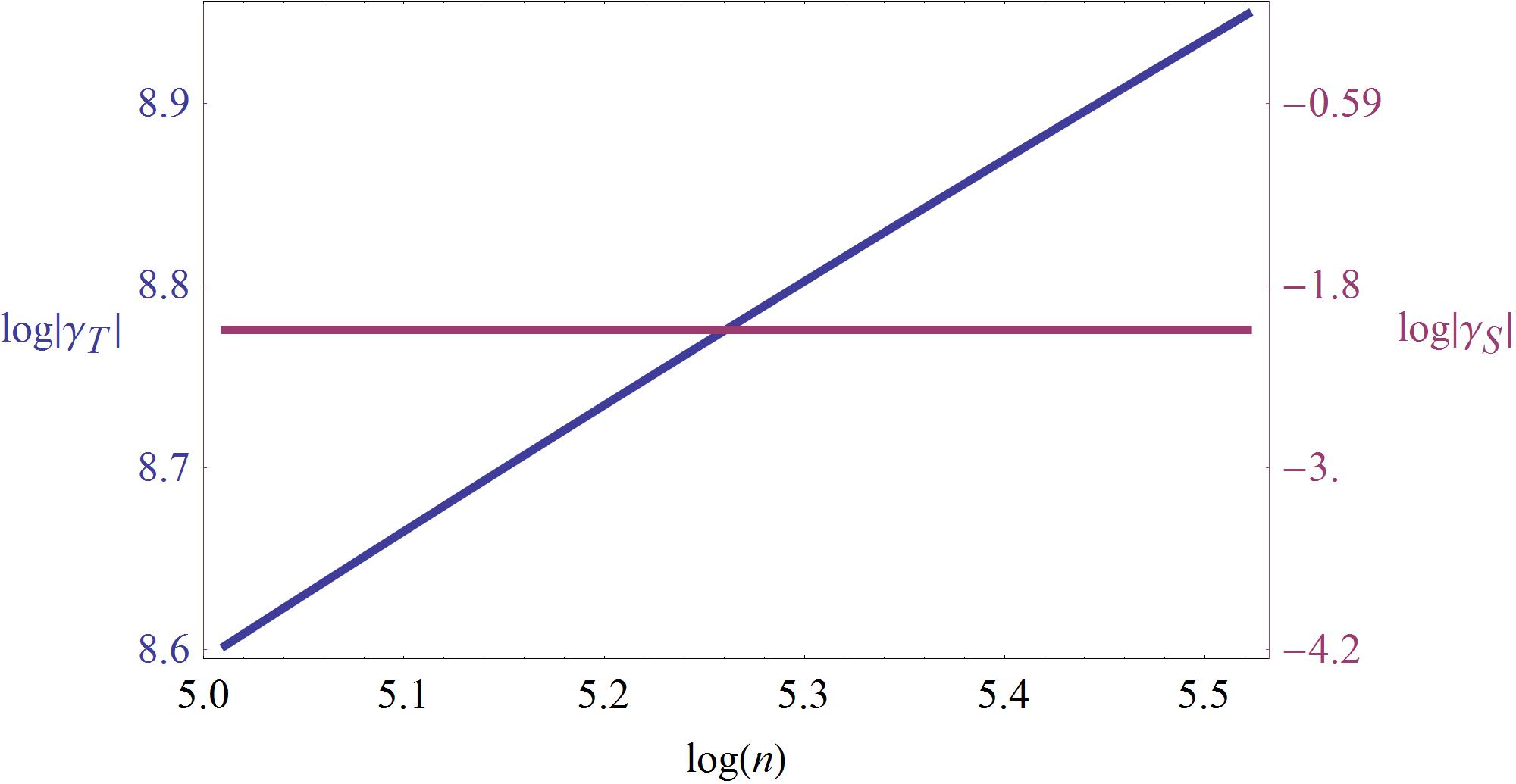
where the extra factor of $\frac{1}{2}$ comes from the normalization $2^{2\ell+\tau-1}$ when we consider the large $\ell$ approximation of the conformal blocks. Equating the coefficients $R_{n}=L_{n}$ we can find the corresponding coefficients $\gamma_{n}$. Thus, in principle, we would know $\gamma_{n}$ if we know $\gamma_{k}$ for all $k\leq n-1$. In figure (2) we have plotted the $\log\gamma_{n}$ vs. $\log n$ for a twist-$2$ scalar and a twist-$2$ and spin-$2$ field.

We find that the slope of the curve for the twist-$2$, spin-$2$ exchange is $\approx 4$ while that for the twist-$2$ scalar is a constant. So $\gamma_{n}\sim n^{4}$ for large values of $n$ for spin-$2$ field. To show this behavior explicitly, we notice that $\gamma_{n}$ can be written as an exact sum over the coefficients $R_{m}$ appearing on the lhs. This formula can be guessed by looking at the first few $\gamma_{n}$s. We give the form of the first few $\gamma_{n}$s. These take the form⁵⁵ 5 We will assume $\Delta_{\phi}>1$. See footnote 4.,

$\displaystyle\begin{split}\gamma_{0}&=\frac{(\Delta_{\phi}-1)^{2}}{8}L_{0}\,,\\ \gamma_{1}&=-\frac{(\Delta_{\phi}-1)^{2}}{8}L_{0}+\frac{\Delta_{\phi}-1}{4}L_{1}\,,\\ \gamma_{2}&=\frac{(\Delta_{\phi}-1)^{2}}{8}L_{0}-\frac{2\Delta_{\phi}-1}{4}L_{1}+\frac{2\Delta_{\phi}-1}{2\Delta_{\phi}}L_{2}\,\ \text{etc.}\end{split}$

(3.8)

We observe that the above terms follow a definite pattern which can be written as,

$$\gamma_{n}=\sum_{m=0}^{n}a_{n,m}\hskip 28.45274pt\text{with}\hskip 28.45274pta_{n,m}=c_{n,m}L_{m}\,.$$

(3.9)

where for general $\tau_{m}$ and $\ell_{m}$ the coefficients $c_{n,m}$ are given by,

$$c_{n,m}=\frac{1}{8}\left(\frac{\Gamma\left(\Delta_{\phi}\right)}{\Gamma\left(\Delta_{\phi}+m-1\right)}\right)^{2}\frac{\left(2\Delta_{\phi}+n-3\right)_{m}(-1)^{n+m}n!}{(n-m)!}\bigg(\frac{\Gamma(\Delta_{\phi}-1)}{\Gamma(\Delta_{\phi}-\tau_{m}/2)}\bigg)^{2}\,.$$

(3.10)

We have checked the analytic expression for the coefficients $\gamma_{n}$ agrees with the solutions of $\gamma_{n}$ found from solving the equations $R_{k}=L_{k}$ order by order for arbitrary values of $n$.

So far we have concentrated on the leading $n$ dependence in the anomalous dimensions for large spin operators, when the lhs of the bootstrap equation is dominated by the stress tensor exchange. Let us now see how to derive the first subleading term with the stress tensor exchange. In [20], this problem for leading twist was considered. By considering large twists we will extract universal results. It turns out that just keeping the leading $\ell$ dependence of the rhs is not sufficient anymore. We will assume a $1/N$ expansion so that we can use the $1/\ell$ corrections in $P^{MFT}$–without the large $N$ we would need to keep track of corrections to these coefficients as well. In $P^{MFT}$ the subleading corrections at large $\ell$ take the form,

$$P^{MFT}=\frac{\sqrt{\pi}\ell^{2\Delta_{\phi}-3/2}}{2^{2\Delta_{\phi}+2\ell}}\bigg[q_{\Delta_{\phi},n}+\frac{1}{\ell}r_{\Delta_{\phi},n}\bigg]\,,$$

(4.1)

where the coefficients $q_{\Delta_{\phi},n}$ and $r_{\Delta_{\phi},n}$ are given by,

	$\displaystyle q_{\Delta_{\phi},n}$	$\displaystyle=\frac{8(\Delta_{\phi}-1)_{n}{}^{2}}{(2\Delta_{\phi}+n-3)_{n}\Gamma(n+1)\Gamma(\Delta_{\phi})^{2}}\,,$
	$\displaystyle r_{\Delta_{\phi},n}$	$\displaystyle=\frac{(\Delta_{\phi}-1)_{n}{}^{2}}{(2\Delta_{\phi}+n-3)_{n}\Gamma(n+1)\Gamma(\Delta_{\phi})^{2}}[5-20\Delta_{\phi}+16\Delta_{\phi}^{2}+4n(4\Delta_{\phi}-3)]\,.$		(4.2)

The conformal blocks in the crossed channel, in the large $\ell$ and $u\rightarrow 0$ limit is,

$$g_{\tau,\ell}(v,u)\overset{\ell\gg 1}{\underset{u\ll 1}{\approx}}k_{2\ell+\tau}(1-z)v^{\tau/2}F^{(d)}(\tau,v)\,,$$

(4.3)

where we have neglected the second term in above expression since even at subleading order in $\ell$, those terms will be exponentially suppressed. We can write $k_{2\ell+\tau}(1-z)$ as follows,

$$k_{2\ell+\tau}(1-z)=\frac{\Gamma(2\ell+\tau)}{\Gamma(\tau/2+\ell)^{2}}\int_{0}^{1}\frac{dt}{t(1-t)}\bigg(\frac{(1-z)t(1-t)}{1-t(1-z)}\bigg)^{\ell+\tau/2}\,.$$

(4.4)

As we show in the appendix (D), for $\ell\gg n\gg 1$,

$$k_{2\ell+\tau}(1-z)=\frac{\Gamma(2\ell+\tau)}{\Gamma(\ell+\frac{\tau}{2})^{2}}K_{0}((2\ell+\tau)\sqrt{z})+O(z)\,.$$

(4.5)

We can further approximate the $K_{0}$ function in the limit of small $\tau/\ell$ upto first order and similarly for the $\Gamma$-functions. The relevant part of the conformal block in the crossed channel takes the form,

$$k_{2\ell+\tau}(1-z)=\frac{2^{2\ell+\tau-1}}{\sqrt{\pi}}\ell^{1/2}\bigg[1+\frac{2\tau-1}{8\ell}\bigg][K_{0}(2\ell\sqrt{z})-\sqrt{z}\tau K_{1}(2\ell\sqrt{z})]\,.$$

(4.6)

Upto this order is sufficient for the calculation of the first subleading order in $z$ after $z^{\tau_{m}/2}$. Let us assume that the anomalous dimensions can be expanded in the form,

$$\gamma(n,\ell)=\frac{\gamma^{0}_{n}}{\ell^{\tau_{m}}}+\frac{\gamma^{1}_{n}}{\ell^{\tau_{m}+1}}+\frac{\gamma_{n}^{2}}{\ell^{\tau_{m}+2}}+\dots\,.$$

(4.7)

¿From the first subleading correction we should be able to determine $\gamma^{1}_{n}$. We already know the coefficient $\gamma_{n}^{0}$ as an exact function of $n$ and $\Delta_{\phi}$. Similar to the leading order case, we can perform the large $\ell$ summation (as an integral) and then evaluate the coefficients of the subleading powers of $z$ resulting from these extra terms. On the lhs, the subleading powers of $z$ take the form,

$$1+\frac{1}{4}P_{m}z^{\tau_{m}/2}g_{\tau_{m},\ell_{m}}(u,v)=1+z^{\tau_{m}/2}f_{1}(v)\log v+z^{\tau_{m}/2+1}f_{2}(v)\log v+O(z^{\tau_{m}/2+2})\,.$$

(4.8)

Thus on the lhs only integer powers of $z$ are there in the subleading pieces. Whereas on the rhs, after the large $\ell$ integral, the first subleading power after the leading term in $z^{\tau_{m}/2}$ begins with $z^{(\tau_{m}+1)/2}$ with the coefficient,

	$\displaystyle z^{(\tau_{m}+1)/2}\sum_{n}[(1-2\Delta_{\phi}+(2n+2\Delta_{\phi})\tau_{m})\gamma_{n}^{0}+2\gamma_{n}^{1}]$	$\displaystyle\frac{(\Delta_{\phi}-1)_{n}{}^{2}\Gamma(\Delta_{\phi}-\frac{1}{2}-\frac{\tau_{m}}{2})^{2}}{2\Gamma(n+1)\Gamma(\Delta_{\phi})^{2}\Gamma(2\Delta_{\phi}+n-3)_{n}}$
		$\displaystyle\times v^{n}\log v\ F^{(d)}[2\Delta_{\phi}+2n,v]\,.$		(4.9)

Since there is no $z^{(\tau_{m}+1)/2}$ term on the lhs, we must have for large $n$,

$$\gamma_{n}^{1}=-n\tau_{m}\gamma_{n}^{0}\,.$$

(4.10)

Thus specializing to the case of $\tau_{m}=2$ (stress tensor), to the first subleading order in $\ell$ we have for the anomalous dimensions,

$$\gamma(n,\ell)=\gamma^{0}(n,\ell)\bigg(1-\frac{2n}{\ell}\bigg)\,.$$

(4.11)

where $\gamma^{0}(n,\ell)=-4n^{4}/(N^{2}\ell^{2})$. The main result of [20] is still consistent with this finding⁷⁷ 7 We thank Fernando Alday for the following observation.. For $n=0$ for large $\ell$ the Casimir is $j^{2}\approx\ell^{2}$. For general $n$ the Casimir will become $j^{2}\approx(\ell+n)^{2}$. The main conclusion of [20] is that only even powers of $j$ should appear in the large spin limit–this was explicitly shown for leading twists. In terms of $j$ (for $\tau_{m}=2$) we could have $1/j^{2}\sim 1/(\ell+n)^{2}$ or $1/(j^{2}-n^{2})\sim 1/(\ell(\ell+2n))$ so that in the $j$ variable only even powers of $j$ appear–both these forms are compatible with the subleading term we have derived. We will find the latter behaviour in what follows which is also consistent with the results of [16] for the supersymmetric ${\mathcal{N}}=4$ case.

References

• [1] R. Rattazzi, V. S. Rychkov, E. Tonni and A. Vichi, JHEP 0812, 031 (2008) [arXiv: 0807.0004].
R. Rattazzi, S. Rychkov, and A. Vichi, Phys. Rev. D 83 046011 (2011) [arXiv: 1009.2725].
R. Rattazzi, S. Rychkov, and A. Vichi, J. Phys. A 44 035402 (2011) [arXiv: 1009.5985].
D. Pappadopulo, S. Rychkov, J. Espin and R. Rattazzi, Phys. Rev. D 86 105043 (2012) [arXiv: 1208.6449].
D. Poland, D. Simmons-Duffin and A. Vichi, JHEP 1205, 110 (2012) [arXiv:1109.5176 [hep-th]].
Y. Nakayama and T. Ohtsuki, Phys. Lett. B 734, 193 (2014) [arXiv:1404.5201 [hep-th]].
• [2] I. Heemskerk, J. Penedones, J. Polchinski and J. Sully, JHEP 0910 (2010) 079 [arXiv: 0907.0151[hep-th]].
• [3] M. Hogervorst, H. Osborn and S. Rychkov, JHEP 1308 (2013) 014 [arXiv: 1305.1321[hep-th]].
M. Hogervorst and S. Rychkov, Phys. Rev. D D87 (2013) 106004 [arXiv: 1303.1111[hep-th]].
• [4] F. A. Dolan and H. Osborn, Nucl. Phys. B 629 (2002) 3-73 [hep-th/0011040].
F. A. Dolan and H. Osborn, Annals Phys. 321 (2006) 581-626 [hep-th/0309180].
F. A. Dolan and H. Osborn, [arXiv: 1108.6194[hep-th]].
• [5] C. Beem, L. Rastelli and F. Passerini, Phys. Rev. Lett. 111 (2013) 071601 [arXiv: 1304.1803[hep-th]].
C. Beem, M, Lemos, P. Liendo, L. Rastelli and B. C.  van Rees, [arXiv: 1412.7541[hep-th]].
F. A. Dolan, M. Nirschl and H. Osborn, Nucl. Phys. B 749 (2006) 109-152 [hep-th/0601148].
F. A. Dolan and H. Osborn, Nucl. Phys. B 629 (2002) 3-73 [hep-th/0112251].
F. A. Dolan and H. Osborn, Nucl. Phys. B 593 (2001) 599-633 [hep-th/0006098].
• [6] S. El-Showk, M. F. Paulos, D. Poland, S.  Rychkov, D. Simmons-Duffins and A. Vichi, Phys. Rev. D 86(2012) 025022 [arXiv: 1203.6064[hep-th]].
S. El-Showk, M. F. Paulos, D. Poland, S.  Rychkov, D. Simmons-Duffins and A. Vichi, J. Stat. Phys. 157(2014) 869 [arXiv: 1403.4545[hep-th]].
F. Kos, D. Poland, D. Simmons-Duffin, JHEP 1411 (2014) 109 [arXiv: 1411.7932[hep-th]].
F. Gliozzi and A. Rago JHEP 1410 (2014) 42 [arXiv: 1403.6003[hep-th]].
• [7] A. L. Fitzpatrick, J. Kaplan, D. Poland and D. Simmons-Duffin, JHEP 1312, 004 (2013) [arXiv:1212.3616 [hep-th]].
• [8] Z. Komargodski and A. Zhiboedov, JHEP 1311, 140 (2013) [arXiv:1212.4103 [hep-th]].
• [9] L. F. Alday and J. M. Maldacena, JHEP 0711, 019 (2007) [arXiv:0708.0672 [hep-th]].
• [10] O. Nachtmann, Nucl. Phys. B 63, 237 (1973).
• [11] G. Vos, arXiv:1411.7941 [hep-th].
• [12] L. Cornalba, M. S. Costa and J. Penedones, JHEP 0709, 037 (2007) [arXiv:0707.0120 [hep-th]].
• [13] L. Cornalba, M. S. Costa, J. Penedones and R. Schiappa, Nucl. Phys. B 767, 327 (2007) [hep-th/0611123].
• [14] L. Cornalba, M. S. Costa, J. Penedones and R. Schiappa, JHEP 0708, 019 (2007) [hep-th/0611122].
• [15] X. O. Camanho, J. D. Edelstein, J. Maldacena and A. Zhiboedov, arXiv:1407.5597 [hep-th].
• [16] L. F. Alday, A. Bissi and T. Lukowski, arXiv:1410.4717 [hep-th].
• [17] G. Arutyunov, F. A. Dolan, H. Osborn and E. Sokatchev, Nucl. Phys. B 665, 273 (2003) [hep-th/0212116].
• [18] A. L. Fitzpatrick, E. Katz, D. Poland and D. Simmons-Duffin, JHEP 1107, 023 (2011) [arXiv:1007.2412 [hep-th]].
• [19] L. F. Alday and A. Bissi, JHEP 1310 (2013) 202 [arXiv: 1305.4604[hep-th]].
• [20] L. F. Alday, A. Bissi and T. Lukowski, [arXiv: 1502.07707[hep-th]].
• [21] A. Kaviraj, K. Sen and A. Sinha, arXiv:1504.00772 [hep-th], to appear in JHEP.