Improved Numerical Cherenkov Instability Suppression in the Generalized PSTD PIC Algorithm
Abstract
The family of generalized Pseudo-Spectral Time Domain (including the Pseudo-Spectral Analytical Time Domain) Particle-in-Cell algorithms offers substantial versatility for simulating particle beams and plasmas, and well written codes using these algorithms run reasonably fast. When simulating relativistic beams and streaming plasmas in multiple dimensions, they are, however, subject to the numerical Cherenkov instability. Previous studies have shown that instability growth rates can be reduced substantially by modifying slightly the transverse fields as seen by the streaming particles . Here, we offer an approach which completely eliminates the fundamental mode of the numerical Cherenkov instability while minimizing the transverse field corrections. The procedure, numerically computed residual growth rates (from weaker, higher order instability aliases), and comparisons with WARP simulations are presented. In some instances, there are no numerical instabilities whatsoever, at least in the linear regime.
Keywords:
Particle-in-cell , Pseudo-Spectral Time-Domain, Relativistic beam , Numerical stability.1 Introduction
The Pseudo-Spectral Time Domain (PSTD) Particle-in-Cell (PIC) algorithm advances Fourier-transformed electromagnetic fields in time according to the difference equations [1],
| (1) |
| (2) |
Simulation particles, of course, require fields and produce currents in real, not Fourier, space. Consequently, Fourier transforms of both fields and currents are performed at each time step. The fields and currents in real space typically are located at the nodes of a regular multidimensional mesh, with magnetic fields and currents offset a half time step from electric fields .
The PSTD algorithm has been generalized by the authors in two ways [2, 3]. First, the components of in Eqs. (1) and (2) are replaced by the Fourier transforms of various order finite difference approximations to spatial derivatives on a grid [4], which has the effect of narrowing the effective width of the particle interpolation stencils. For instance, might be replaced by
yielding a pseudo-spectral realization in k-space of the standard Finite-Difference Time Domain (FDTD) algorithm. (In this context the components of itself can be viewed as an infinite order approximation.) Second, the field solver is modified to increase the relatively small PSTD Courant time step limit by a factor of N, an integer. This modification is equivalent mathematically to sub-cycling the field solver N times but is faster computationally. Note that the generalized PSTD algorithm reduces to Haber’s Pseudo-Spectral Analytical Time-Domain (PSATD) algorithm [5] in the limit of infinite N. Both the details of and the motivation for the generalized PSTD algorithm, dubbed the Pseudo-Spectral Arbitrary Order Time Domain (PSAOTD) algorithm, are described thoroughly in [2].
The numerical Cherenkov instability [6, 7] is observed commonly in PIC simulations of relativistic particle beams and streaming plasmas; e.g., [8, 9, 10], where it can be fast growing and strongly disruptive. At a minimum the instability increases beam emittance [11]. It arises from nonphysical coupling between the usual electromagnetic modes, possible distorted by numerical effects, and spurious beam modes [12, 13]. The dispersion relation describing the numerical Cherenkov instability has the general form,
| (3) |
where the are complicated functions of the instability frequency , wave numbers , time step , cell size, and alias index . The particular form of the is determined by the details of the numerical algorithm, given in [2] for PSAOTD. The relativistic beam itself is characterized by its normalized energy , axial velocity , and normalized relativistic plasma frequency . Of particular importance are the resonances at , with alias wave numbers . (The beam propagates along the z-axis.) Each alias can trigger an instability, with the most rapid growth typically occurring for . High order interpolation, say cubic, significantly reduces growth rates associated with higher order aliases. Although peak growth rates typically occur at large wave numbers, nontrivial growth rates can occur at quite small wave numbers, especially for [12, 13]. The nonresonant instability has two branches [13, 14], the primary branch associated with the term of the dispersion relation, and the secondary branch with the term. The former occurs over a wide range of wave numbers, while the latter occurs at and small , if at all. See Fig. 1. Unless otherwise noted, parameters for these and other figures are , , and . The k-space grid is 65x65, corresponding to a simulation grid of 128x128.
Until recently, the numerical Cherenkov instability was ameliorated by a combination of digital filtering, numerical damping, higher order interpolation (typically cubic), and astute parameter choices [8, 15]. Papers within the past few years have offered alternative options, often entailing minor corrections to the transverse electric and magnetic fields as seen by the particles [2, 3, 13, 16]. Specifically, transverse electric and magnetic fields as they are interpolated to the particles are multiplied by -dependent correction factors and that vary as for small . The distinction between such correction factors and the usual digital filters is made clear in [13, 17]. The particular analytical correction factors presented in these references are quite effective at ameliorating the first branch of the instability but ineffective at ameliorating the second, for reasons presented later in this article.
As an alternative, this paper numerically computes correction factors and just sufficient to completely eliminate both branches of the numerical Cherenkov instability. The process is straightforward in principle. The dispersion function is akin to a fifth order polynomial with real coefficients. If it crosses the -axis in five places (i.e., five real roots), all roots are stable. However, if parameters are varied such that the curve crosses the axis in only three places or one, then the dispersion function has two or four complex roots, respectively, the remaining roots being real. The transition occurs where the curve becomes tangential to the -axis, i.e., where both the dispersion function and its derivative with respect to vanish. This determines and . In fact, it can be shown that the portion of Eq. (3) can be represented as a fifth order polynomial, although this is not required for the argument of this paragraph to be true.
Fig. 2, computed for and , is illustrative. The left plot displays the dispersion function, Eq. (3) with only, for the complete frequency range, . Shown are the results for the uncorrected case, (labeled Base), for the correction factors described in [2] (labeled ), and for the numerically determined optimal correction factors (labeled Opt). (The correction factors are chosen so that the term vanishes at ). The three curves are essentially indistinguishable on this scale, with one crossing at the far left and two or four crossings at the right. The right plot displays a blow-up of the critical frequency range. Each curve has one crossing in this range, and a second crossing is off-scale to the right. However, the Opt curve is seen also to be tangent to the -axis at a point. Hence, it is stable, and the other two cases are not. The corresponding instability growth rates are 0.0749, 0.0014, and 0 for Base, , and Opt.
The next section provides sample numerical correction factors and the procedure used to obtain them. The third section then provides corresponding numerical growth rates from Eq. (3), along with corroborating instability growth rates from WARP two-dimensional simulations [18]. A short concluding section completes the paper.
The analytical and numerical linear growth rate analyses were performed using Mathematica [19].
2 Numerical Procedure for Obtaining and
The factors and appear linearly in the dispersion function, obtained from Eq. 3 by omitting all but the terms in the summations, and in its derivative with respect to . As a consequence, the dispersion function and its derivative together can be inverted readily to obtain and as functions of the tangent point, , although the actual expressions are quite complicated.
Fig. 3 (left) is a typical parametric plot of vs. as is varied. Its parameters are identical to those of Fig. 2. The region below the diagonal curve is stable, above it unstable. (Despite appearances, it bends slightly and does not pass through the origin.) Although any choice of and along or below this curve stabilizes the mode, a pair close to (1,1) is to be preferred for minimizing numerical impact on the physics to be simulated. Further constraining the choice by , suggests the following procedure:
- 1.
If numerical instability growth is zero at (1,1), set , .
- 2.
Otherwise, search the lines and for the point nearest (1,1) at which the dispersion function and its derivative simultaneously vanish. Usually, that point will be on the line, as illustrated in the left plot of Fig. 3.
- 3.
Otherwise, search for the point nearest (1,1) at which the dispersion function and its derivative simultaneously vanish in the interior of the region. It is fortunate that this situation is rare, because such points are expensive to find computationally and easy to miss.
- 4.
Otherwise, set . The numerical instability cannot be eliminated, short of excising that portion of -space.
For completeness, Fig. 3 (right) provides the parametric plot of vs. for , which lies at the center of the second branch of the numerical Cherenkov instability in Fig. 1. Stable regions lie above the upper diagonal curve and below the lower diagonal curve. Only a very small reduction from unity in is sufficient to eliminate the numerical instability.
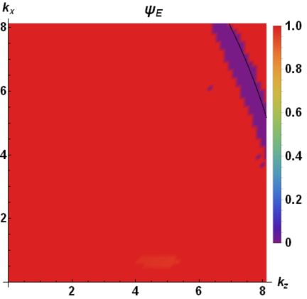
Plots of and for the parameters of Fig. 2 are shown in Fig. 4 with the resonance curve superimposed. is equal to unity everywhere but (1) in the small region, barely visible at the bottom center of the plot, where the second branch of the numerical Cherenkov instability appears in Fig. 1, (2) near the resonance curve, where , and (3) at three isolated points where also. for the second branch of the numerical instability. In contrast, everywhere except those values where the growth rate is zero anyway. Note that over a wide range of small .
The three isolated points appearing in both plots are associated with a weak instability predicted by Birdsall and Langdon in Problem 5-9a of their well known text [20]. Because this instability has a very narrow bandwidth in k-space, it appears only where the instability band happens to overlap nodes on the k-space numerical grid. Analysis of this Courant-like instability for the generalized PSTD algorithm is provided in [2], and analysis plus growth rates for the PSATD algorithm in [16]. This instability appears to be unimportant in practice except, perhaps, at low .
Applying the correction factors of Fig. 4 for the parameters used to obtain Fig. 1 completely eliminates numerical instability growth but has minimal effect on higher order aliases except for -space regions where or are much less than unity. Hence, we choose to truncate fields in -space according to
| (4) |
in order to minimized peak growth rates of the first branch of the instability. Fig. 5 (left) displays the resulting growth rates for . Truncating -space according to Eq. (4) reduces the peak growth rate from 0.168 to 0.071, and the Fig. 4 correction factors further reduce it to 0.026. Most of the residual growth is associated with the second branch. The second branch of the numerical Cherenkov instability is absent, as expected. In contrast, Eq. (4) with correction factors reduces peak growth comparably, but with nontrivial growth rates spread over a larger range in -space; see Fig. 5 (right). In particular, it causes the second branch of the numerical instability to shift toward but does nothing to eliminate it. This is because the topology of the vs. parametric plot changes rapidly for very small near this second instability branch. As a consequence, slightly reducing there actually can create an instability where none otherwise exists.
3 Numerical Instability Growth Rates
Although -space truncation with yields reasonably effective instability suppression, is much better. Additionally, choosing better accommodates comparisons with earlier papers [16, 3, 2]. Fig. 6 (left) depicts peak growth rates for , the last being PSATD. Peak growth rates are relatively insensitive to N. As always, the rapid variation of peak growth with reflects the rapidly changing locations of higher order resonances on the -space grid. Note that the largest growth rates are associated with =0.9 , used as the sample case in the preceding Section. No growth whatsoever is predicted for , because all aliases coincide there. Peak growth rates for and various order finite difference approximations to are shown in Fig. 6 (right). Results are similar to those in the left plot. Superimposed on the growth rate curves are results from several WARP simulations [18]. Agreement is very good. In addition, a simulation was run to for with no sign of instability growth. However, at still larger values of time, instability growth at a rate of about 0.003 developed at wave numbers consistent with the second branch of the numerical Cherenkov instability. Perhaps, a slight change in the beam distribution function over time moved this instability above threshold. If so, reducing very slightly there might prevent this very late time growth.
The procedure introduced in this paper remains robust at low . Fig. 7 presents peak growth rates for , , , and infinite order. Results are comparable to the best obtained earlier; see Fig. 7 of [16]. Both here and in [16], is offset by one-half cell to suppress the usual quasi-electrostatic numerical instability that occurs at low [21, 22, 23]. The peak in Fig. 7 at is larger than that in Fig. 6 only because is larger.
4 Conclusion
New field correction factors have been derived that completely eliminate the numerical Cherenkov instability for the generalized PSTD algorithm, including the PSATD algorithm. When combined with a sharp cutoff digital filter at large , these correction factors reduce peak growth rates to less (often much less) than 0.01 of the beam’s relativistic plasma frequency. These coefficients are optimal in the sense that they differ from unity only slightly over a broad portion of -space while eliminating both numerical instability branches. A disadvantage from the implementation perspective is that the coefficients must be computed numerically for each set of simulation parameters. Software for doing so is available in Mathematica CDF format [24] at http://hifweb.lbl.gov/public/BLAST/Godfrey/.
Acknowledgment
We thank Irving Haber for suggesting this collaboration and for helpful recommendations. We also are indebted to David Grote for assistance in using the code WARP. This work was supported in part by the Director, Office of Science, Office of High Energy Physics, U.S. Dept. of Energy under Contract No. DE-AC02-05CH11231 and the US-DOE SciDAC ComPASS collaboration, and used resources of the National Energy Research Scientific Computing Center.
This document was prepared as an account of work sponsored in part by the United States Government. While this document is believed to contain correct information, neither the United States Government nor any agency thereof, nor The Regents of the University of California, nor any of their employees, nor the authors makes any warranty, express or implied, or assumes any legal responsibility for the accuracy, completeness, or usefulness of any information, apparatus, product, or process disclosed, or represents that its use would not infringe privately owned rights. Reference herein to any specific commercial product, process, or service by its trade name, trademark, manufacturer, or otherwise, does not necessarily constitute or imply its endorsement, recommendation, or favoring by the United States Government or any agency thereof, or The Regents of the University of California. The views and opinions of authors expressed herein do not necessarily state or reflect those of the United States Government or any agency thereof or The Regents of the University of California.
References
References
- [1] Q. Liu, The pstd algorithm: A time-domain method requiring only two cells per wavelength, Microwave and Optical Technology Letters 15 (3) (1997) 158–165.
- [2] J.-L. Vay, B. B. Godfrey, Pseudo-spectral arbitrary order time domain algorithm, in preparation.
- [3] B. B. Godfrey, Review and recent advances in pic modeling of relativistic beams and plasmas, in: Proceeding of 2014 Advanced Accelerator Concepts Workshop, 2014.
- [4] S. Lele, Compact finite difference schemes with spectral-like resolution, Journal of Computational Physics 103 (1992) 16–42.
- [5] I. Haber, R. Lee, H. Klein, J. Boris, Advances in electromagnetic simulation techniques, in: Proc. Sixth Conf. Num. Sim. Plasmas, Berkeley, CA, 1973, pp. 46–48.
- [6] B. B. Godfrey, Numerical cherenkov instabilities in electromagnetic particle codes, Journal of Computational Physics 15 (4) (1974) 504–521.
- [7] B. B. Godfrey, Canonical momenta and numerical instabilities in particle codes, Journal of Computational Physics 19 (1) (1975) 58–76.
- [8] J.-L. Vay, C. G. R. Geddes, E. Cormier-Michel, D. P. Grote, Numerical methods for instability mitigation in the modeling of laser wakefield accelerators in a lorentz-boosted frame, Journal of Computational Physics 230 (15) (2011) 5908–5929. doi:10.1016/j.jcp.2011.04.003.
- [9] L. Sironi, A. Spitkovsky, private Communication (2011).
- [10] X. Xu, P. Yu, S. F. Martins, F. Tsung, V. K. Decyk, J. Vieira, R. A. Fonseca, W. Lu, L. O. Silva, W. B. Mori, Numerical instability due to relativistic plasma drift in em-pic simulations, Computer Physics Communications 184 (2013) 2503–2514.
- [11] E. Cormier-Michel, B. Shadwick, C. Geddes, E. Esarey, C. Schroeder, W. P. Leemans, Unphysical kinetic effects in particle-in-cell modeling of laser wakefield accelerators, Physical Review E 78 (2008) 016404. doi:10.1103/PhysRevE.78.016404.
- [12] B. B. Godfrey, J.-L. Vay, Numerical stability of relativistic beam multidimensional pic simulations employing the esirkepov algorithm, Journal of Computational Physics 248 (2013) 33–46. doi:10.1016/j.jcp.2013.04.006.
- [13] B. B. Godfrey, J.-L. Vay, I. Haber, Numerical stability analysis of the pseudo-spectral analytical time-domain pic algorithm, Journal of Computational Physics 258 (2014) 689–704. doi:10.1016/j.jcp.2013.10.053.
- [14] P. Yu, X. Xu, V. K. Decyk, F. Fiuza, J. Vieira, F. Tsung, R. A. Fonseca, W. Lu, L. O. Silva, W. B. Mori, Elimination of the numerical cerenkov instability for spectral em-pic codes, arXiv:1407.0272v2.
- [15] P. Yu, X. Xu, V. K. Decyk, W. An, J. Vieira, F. Tsung, R. A. Fonseca, W. Lu, L. O. Silva, W. B. Mori, Modeling of laser wakefield acceleration in lorentz boosted frame using em-pic code with spectral solver, Journal of Computational Physics 266 (2014) 124–138. doi:10.1016/j.jcp.2014.02.016.
- [16] B. B. Godfrey, J.-L. Vay, I. Haber, Numerical stability improvements for the pseudo-spectral em pic algorithm, IEEE Transactions on Plasma Science 42 (5) (2014) 1339–1344. doi:10.1109/TPS.2014.2310654.
- [17] B. B. Godfrey, J.-L. Vay, Suppressing the numerical cherenkov instability in fdtd pic codes, Journal of Computational Physics 267 (2014) 1–6. doi:10.1016/j.jcp.2014.02.022.
- [18] D. Grote, A. Friedman, J.-L. Vay, I. Haber, The warp code: modeling high intensity ion beams, in: AIP Conference Proceedings, no. 749, 2005, pp. 55–58.
- [19]
Mathematica, version ten (2014).
URL http://www.wolfram.com/mathematica/ - [20] C. K. Birdsall, A. B. Langdon, Plasma physics via computer simulation, Taylor & Francis, 2005.
- [21] C. K. Birdsall, N. Maron, Plasma self-heating and saturation due to numerical instabilities, Journal of Computational Physics 36 (1980) 1–19. doi:10.1016/0021-9991(80)90171-0.
- [22] H. R. Lewis, Variational algorithms for numerical simulation of collisionless plasma with point particles including electromagnetic interactions, Journal of Computational Physics 10 (3) (1972) 400–419.
- [23] A. B. Langdon, Energy-conserving plasma simulation algorithms, Journal of Computational Physics 12 (2) (1973) 247–268.
- [24]
Computable document format (cdf)
(2014).
URL http://www.wolfram.com/cdf-player/