Environmental gravitational decoherence
and a tensor noise model

In this section, we follow notations used in [15]. The total action of a mass distribution which is centered around $\mathbf{x}_{0}$ and coupled to gravity can be written as

The action $S_{\rm grav}(h_{\mu\nu})$ contains in general also gravitational self-interaction terms which are of higher order and will not be considered here. We choose the transverse-traceless gauge, i.e., $h_{0\mu}=h^{ij}_{\hskip 5.69046pt,i}=h^{i}_{\hskip 2.84544pti}=0$. Then the graviton action adopts the simple quadratic form

The interaction between the energy-momentum tensor $T^{ij}_{\mathbf{x}_{0}}$ of the system and the external graviton field is bilinear, i.e.,

Here only the spatial components of the energy-momentum tensor contribute due to the gauge choice above. The graviton field can be expanded into plane waves according to

where we introduced the transverse-traceless polarization tensors $\epsilon^{\lambda}_{ij}(\mathbf{k})$. The time-evolution of the system’s density matrix is determined by the action $S_{\mathrm{sys}}(\mathbf{x}_{0})$ and the influence functional $\mathcal{F}(\mathbf{x}_{0},\mathbf{x}_{0}^{\prime})$. Then the propagator of the reduced density matrix is given by

where the subscripts $i,f$ indicate the initial and final values respectively. The influence functional adopts the explicit form

with the correlation functions

We assumed the environmental modes to be in a thermodynamical state with the inverse temperature $\beta$. The sum over polarizations gives the polarization tensor $\sum_{\lambda}\epsilon^{\lambda}_{ij}(\mathbf{k})\epsilon^{\lambda*}_{kl}(\mathbf{k})=\Pi_{ij,kl}(\mathbf{k})=P_{ik}P_{jl}+P_{il}P_{jk}-P_{ij}P_{kl}$ where the projection operators are $P_{ij}=\delta_{ij}-\frac{k_{i}k_{j}}{|\mathbf{k}|^{2}}$.

The real and imaginary parts of the phase $\phi$ in the influence functional (2.1) lead to dissipation and decoherence, respectively. In this section, we calculate

from which the dependence of the decoherence rate on the various parameters of the model follows. As particular example, we discuss the evaluation of (8) using an interference device setup (Figure 2). A matter distribution is in superposition of either following a right trajectory $\mathbf{x}_{0}$ (blue) or a left one $\mathbf{x}^{\prime}_{0}$ (red). For a small angle $\theta$, Figure 2 can be interpreted as the double-slit experiment, whereas $\theta=\frac{\pi}{2}$ corresponds to an interferometer. On both trajectories, the system changes its direction at time $t=t_{\rm kick}$ due to a slit or mirror. The energy-momentum tensor of a particle in flat space-time takes the form

with the velocity vector $v_{\mu}(t)=(1,\mathbf{v}_{0}(t))$. We assume that a particle is smeared out over a space-region determined by $\sigma$, i.e., $\delta_{\sigma}(\mathbf{x})=\frac{1}{(2\pi\sigma^{2})^{3/2}}\exp\left[-\frac{\mathbf{x}^{2}}{2\sigma^{2}}\right]\,.$

It is well-known that the divergence equation of the energy-momentum tensor gives the geodesic equation with respect to the background space-time. However, the two possible trajectories of a particle in Figure 2 do not correspond to geodesics in Minkowski space-time, hence $\partial_{\nu}T_{\mathrm{part},\mathbf{x}_{0}}^{\mu\nu}\neq 0$. Generally, one would need to model a mirror, the interaction between a particle and a mirror and the interaction of gravity with the particle-mirror system. Here, we follow a simpler approach by adding momentum densities which kick a particle at $t=t_{\rm kick}$. Thus, our system can be described now as “particle + momentum density such that the energy-momentum tensor is divergence-free along the trajectories”. In particular, we choose

The time-time component $T_{\mathrm{mom},\mathbf{x}_{0}}^{00}(x)$ can be chosen such that

The additional momentum densities ensure that the divergence of the energy-momentum tensor $T_{\mathbf{x}_{0}}^{\mu\nu}=T_{\mathrm{part},\mathbf{x}_{0}}^{\mu\nu}+T_{\mathrm{mom},\mathbf{x}_{0}}^{\mu\nu}$ vanishes along the trajectory.

In order to obtain an interpretation of the momentum densities introduced, let us consider $\mathbf{v}_{0}(s)=v_{1}(s)\hat{\mathbf{x}}+v_{2}\hat{\mathbf{y}}$ with $v_{1}(s)=v\sin(\theta/2)\theta(t_{\rm kick}-s)-v\sin(\theta/2)\theta(s-t_{\rm kick})$ and $v_{2}=v\cos(\theta/2)$. Then we have

We interpret this expression as follows: When $t<t_{\rm kick}$, a particle moves straight in positive $\hat{\mathbf{x}}$- and $\hat{\mathbf{y}}$-directions. At time $t_{\rm kick}$, it gets a momentum transfer which changes its velocity in $\hat{\mathbf{x}}$-direction from $v\sin(\theta/2)$ to $-v\sin(\theta/2)$. This corresponds to the right trajectory $\mathbf{x}_{0}$ in Figure 2. A left trajectory $\mathbf{x}_{0}^{\prime}$ which has a kick at $t_{\rm kick}$ towards the right can be constructed in the same way by defining $\mathbf{v}^{\prime}_{0}(s)=-v_{1}(s)\hat{\mathbf{x}}+v_{2}\hat{\mathbf{y}}$.

By substituting $T_{\mathbf{x}_{0}}^{\mu\nu}=T_{\mathrm{part},\mathbf{x}_{0}}^{\mu\nu}+T_{\mathrm{mom},\mathbf{x}_{0}}^{\mu\nu}$ into (8) and evaluating the thermal part of the expression (8) along the trajectories, we find for velocities $v\ll 1$

where $T$ is a time when two trajectories meet again. With an angle $0<\theta<\pi$, the effect is approximately proportional to $v^{4}$. The authors of [16] found the same velocity-dependence in the non-relativistic single-mode limit from a master equation approach. When $\pi T/(2\beta)\gg 1$ and $\theta=\pi/2$, we have

The decoherence factor $\mathrm{Im}(\phi)$ vanishes when two trajectories are parallel $\theta=0$, that is, the trajectories coincide with each other. With $\theta=\pi$, $\mathrm{Im}(\phi)$ is proportional to $v^{6}$,

Apart from thermal gravitational waves, vacuum fluctuations also contribute to the decoherence rate. For realistic parameters, this contribution is very small that it can be neglected. Its expression diverges logarithmically with the inverse of the spread of the mass distribution, $1/\sigma$.

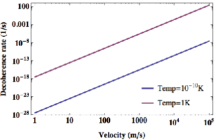
In Figure 2, we plotted the decoherence rate with the temperature of the gravitational waves being 1K and $10^{-10}$K. Since gravitational waves decoupled earlier from photons and have therefore a lower temperature than the Cosmic Microwave background. However, the actual temperature of the thermal gravitational waves background can be much lower and it depends on the details of reheating after inflation [17]. Here, we assume a thermal contribution with 1K as the upper bound and vacuum contribution would be the lower bound on the decoherence rate.

We claim that the decoherence effect comes along with the emission of gravitational waves. The emitted energy of a particle along one of the trajectories depicted in Figure 2 can be calculated classically. The emission occurs when the direction of a particle is changed by a mirror. As long as the emitted radiation can be distinguished for trajectories, the environment measures which path a particle is moving to some extent, and this leads to environmental gravitational decoherence.

For a trace-reversed perturbation, $\bar{h}_{\mu\nu}^{\mathrm{pert}}=\bar{h}_{\mu\nu}^{\mathrm{pert}}-\bar{h}^{\mathrm{pert}}\eta_{\mu\nu}/2$, the solution to the linearized Einstein equations gives the expression

When the particle is slowly moving, the far field is dominated by quadrupole moment tensor $I_{ij}=\int d^{3}x\,x^{i}x^{j}T_{00,\mathbf{x}_{0}}(x)$. In terms of the trace-free quadrupole moment, $J_{ij}=I_{ij}-\delta_{ij}\delta^{kl}I_{kl}/3$, the emitted power is

Here we will assume a smooth trajectory of a particle which moves along one path

with $f(t,s)=(\tanh((t-s)/t_{0})-1)/2$. The time $t_{0}$ determines how fast the direction of a particle is changed at a mirror, how fast a particle is accelerated initially from a source and decelerated at a detector finally. In the limit $T\gg t_{0}$, the radiated energy is crucially determined by $t_{0}$,

For vacuum fluctuations, the minimal possible time $t_{0}$ is determined by the extension of the particle, that is $t_{0,\mathrm{min}}\sim\sigma$. For finite temperatures, the effective cutoff of the gravitational modes is determined by $1/\beta$, so one should expect $t_{0,\mathrm{min}}\sim\beta$.

References

- [1] Marshall W, Simon C, Penrose R and Bouwmeester D 2003 Phys. Rev. Lett. 91 130401
- [2] Kleckner D et al. 2008 New Journal of Physics. 10 095020
- [3] Kaltenbeck R et al. 2012 Exp Astron. 34 123
- [4] Penrose R 1996 General Relativity and Gravitation. 28 581-599
- [5] Penrose R 1986, In Quantum Gravity 2: A Second Oxford Symposium, Oxford University Press
- [6] Penrose R 1986, In Quantum Concepts in Space and Time, Oxford University Press
- [7] Diósi L 1987 Phys. Lett. 120 A 377-381
- [8] Károlyházy F 1966 Nuovo Cim. 52 390
- [9] Károlyházy F 1974, Magyar Fizikai Polyoirat 12 24
- [10] Komar A B 1969, Int. J. Theor. Phys. 2 157
- [11] Omnès R 1992, Rev. Mod. Phys. 64 339
- [12] Unruh W G 2000 In Relativistic quantum measurement and decoherence eds Breuer H P and Petruccione F (Springer) pp 125-140
- [13] Breuer H and Petruccione F 2001 Phys. Rev. A 63 032102-1
- [14] Breuer H and Petruccione F 2002 The Theory of Open Quantum Systems. (Oxford)
- [15] Anastopoulos C 1996 Phys. Rev. D 54 1600
- [16] Anastopoulos C and Hu B L 2013 Class. Quantum Grav. 30 165007
- [17] Hu B L 2014 J. Phys.: Conf. Ser. 504 012021
- [18] Anastopoulos C and Hu B L 2008 Class. Quantum Grav. 25 154003
- [19] Cloutier J and Semenoff G W 1991 Phys. Rev. D 44 3218-3229