FKPP fronts in cellular flows:
the large-Péclet regime

In a wide variety of environmental and engineering applications, chemical or biological reactions in fluids propagate in the form of localized, strongly inhomogeneous structures associated with reactive fronts [43, 29]. These are usually established as a result of the interaction between molecular diffusion, local growth and saturation, but their propagation can be greatly facilitated by advection by a flow. There has been a growing interest in analysing this impact of advection on the propagation of reactive fronts, as indicated by the large number of experimental, and theoretical studies (e.g., [35, 39, 44, 6]) and [48, 7, 49], respectively).

Much of this work focusses on the effect of incompressible two-dimensional periodic flows, and in particular on the cellular vortex flow. Introduced by [11], this is a steady flow with streamfunction

where $U$ is the maximum flow speed and $2\pi\ell$ is the period in both $x$ and $y$. When the system is confined between parallel, impermeable walls at $y=0$ and $\pi\ell$, as considered in this paper, the flow consists of a one-dimensional infinite array of vortices rotating in alternating directions (see Fig. 1). These vortices are confined within cells that are bounded by a separatrix connecting a network of hyperbolic stagnation points.

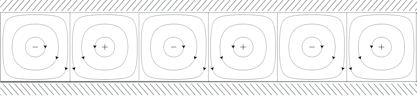
In the absence of advection, the simplest model of front propagation is the FKPP model, named after the pioneering work by Fisher [15] and Kolmogorov, Petrovskii and Piskunov [24]. This model describes the evolution of a single constituent that diffuses and undergoes a logistic growth, leading to the formation of a steadily travelling front. In the presence of a cellular flow (or more general steady periodic flows), the corresponding advection–diffusion–reaction model admits pulsating front solutions that change periodically with respect to time as they travel [8].

The behaviour of these pulsating fronts depends on two non-dimensional parameters: the Damköhler and Péclet numbers,

where $\tau$ is the reaction time and $\kappa$ the molecular diffusivity, which measure the strength of advection relative to reaction and to diffusion, respectively. In the interpretation of our results, we will consider a fixed geometry and a fixed flow, in which case the values of Pe and Da are controlled by $\kappa$ and $\tau$, respectively. In practice, however, it is easier to achieve this control by varying $\ell$ and $U$ (see e.g. [35]).

This paper focusses on the limit of large Pe, relevant to many applications where advection dominates over diffusion. This is a singular limit, of course, since the weak diffusion leads to the creation of spatial scales that are vanishingly small as $\text{Pe}\to\infty$. These small scales are apparent in Figure 2 which illustrates the dependence of the front structure on the reaction time by showing snapshots of the concentration for different Damköhler number Da at fixed (large) $\text{Pe}=250$. For small Da (slow reaction, Fig. 2(a)), the front spreads across several cells, with high concentrations within boundary layers surrounding the separatrix. For intermediate Da (Fig. 2(b)), the front is narrower: its leading edge is confined around the separatrix as it invades successive cells. For large Da (fast reaction, Fig. 2(c)), the front is very sharp with a leading edge that penetrates into the cell interiors.

The main quantitative characteristic of the front is its long-time speed, $c$. This speed is a function of Da and Pe only when the initial conditions are sufficiently close to a step function. Assuming this, Freidlin and Gärtner [19] showed that $c$ can be deduced from the principal eigenvalue of a certain linear operator. This eigenvalue can be interpreted in the framework of large-deviation theory: specifically, it is the Legendre dual of the rate function $g(c)$ associated with the probability density function for the position of fluid particles that have been displaced – by advection and diffusion – to a distance $ct$ in a time $t\gg 1$. Intuitively, these particles control the concentration near the leading edge of the front which, by linearisation, is approximately of the form $\exp(-t(g(x/t)-\text{Da}))$, whence the front speed $c=x/t=g^{-1}(\text{Da})$ is obtained. An alternative approach, based on the minimum speed of propagation, leads to the same eigenvalue problem, as established in [47, 9].

The eigenvalue problem does not provide an explicit analytical expression for the front speed but needs to be solved numerically, through computations that become increasingly intensive as $\text{Pe}\to\infty$ or $\text{Da}\to\infty$. In the present paper, we carry out a detailed asymptotic analysis of the eigenvalue problem for $\text{Pe}\gg 1$ and arbitrary Da. This provides simpler, and in some cases completely explicit, expressions for the front speed, extracting the dominant scalings and elucidating the physical mechanisms of propagation depending on the relative values of Pe and Da.

Partial results of this type have been derived for slow reaction i.e. for $\text{Da}=O(\text{Pe}^{-1})$: the dimensionless front speed was argued to scale like $c/U=O(\text{Pe}^{-3/4})$ in [5]. This scaling prediction is in agreement with rigorous bounds obtained in [31] and was confirmed by numerical simulations [3, 4, 46]. It is consistent with the closed-form prediction obtained using a homogenization technique which is however only valid for $\text{Da}\ll\text{Pe}^{-1}$. In this regime, $c$ is found to be proportional to the square root of the effective diffusivity deduced from a linear cell problem [12, 42, 22, 38, 50] and determined in [41, 40, 37]. In the opposite limit of fast reaction, i.e. for $\text{Da}=O(\text{Pe})$, $c$ can be deduced from the homogenization of a Hamilton–Jacobi equation [17, 28, 16] and computed by minimizing a certain action functional [45]. The present paper extends these results to provide a complete description of the asymptotics of $c$ as $\text{Pe}\to\infty$.

We carry out an asymptotic analysis of the eigenvalue problem determining $c$ and identify three distinguished regimes, characterised by the value of Da relative to Pe. These three regimes correspond to the three types of fronts depicted in Figure 2. In each regime, we obtain the front speed in terms of a non-trivial function of a combination of Pe and Da (see Table 1). The function relevant to each regime is obtained by solving one-dimensional problems numerically. We moreover show that the three regimes overlap for intermediate values of Da, thus confirming that our results cover the whole range of Da.

Our derivation of $c$ in the first two regimes exploits the matched-asymptotics analysis recently carried out by Haynes and Vanneste [21]. Their paper considers the dispersion of particles in an unbounded cellular flow and derives the rate function $g$ from which we infer $c$ (after some adaptation to account for the walls). The analysis captures the behaviour of the concentration in the interior of the cells at the leading edge of the front. In Regime I, the concentration is found to be nearly constant along the streamlines (see Fig. 2(a)), while in Regime II the concentration is vanishing inside the cell’s interior (see Fig. 2(b)). In both regimes, a boundary layer around the separatrix is crucial for the front dynamics. In Regime III, where the reaction is fast, we rely on a Wentzel–Kramers–Brillouin–Jeffreys (WKB) approach which shows that $c$ is controlled by a single action-minimising trajectory [45].

We note that our predictions are formal, involving no rigorous estimates of the associated errors. Instead, they are verified against values of $c$ derived from (i) numerical solutions of the principal eigenvalue problem, and (ii) direct numerical simulations of the FKPP advection–diffusion–reaction equation. Figure 3 shows that the asymptotic expressions for $c$ are in excellent agreement with the corresponding values obtained from the eigenvalue problem.

There are four subregimes in which the asymptotic expressions for $c$ reduce to closed forms. The reduced expressions, which in fact cover most of the $(\text{Da},\text{Pe})$-plane for $\text{Pe}\gg 1$, are summarised in Table 2. They are used to verify the overlap between regimes mentioned above. In these subregimes, $c$ behaves qualitatively as follows. For $\text{Da}\ll\text{Pe}^{-1}$, the diffusive approximation obtained from classical homogenisation theory is recovered. For $\text{Pe}^{-1}\ll\text{Da}\ll(\log\text{Pe})^{-1}$, $c$ is proportional to $\text{Da}^{3/4}(\log\text{Pe})^{-1/4}$ and is controlled by the dynamics along the separatrix, with the hyperbolic stagnation points at the cell corners playing a negligible role. The range $(\log\text{Pe})^{-1}\ll\text{Da}\ll\text{Pe}$ captures the slow growth of $c$ with Da which, in contrast, can be attributed to the stagnation points. The expression for $c$ in this range can in fact be crudely approximated as the Da-independent $c\sim\pi/\log\text{Pe}$. This is qualitatively similar to the expression obtained in [4, 10] using a heuristic approach based on an alternative model, the so-called G-equation (see also [30] for a more rigorous analysis). To our knowledge, no equivalent expression has previously been derived from the eigenvalue problem. For $\text{Da}\gg\text{Pe}$, the reaction is so strong that advection contributes only a small correction to the well-known FKPP speed $c_{0}=2U\sqrt{\text{Da}/\text{Pe}}=2\sqrt{\kappa/\tau}$.

The paper is structured as follows. In section 3, we give a brief derivation of the eigenvalue problem for the front speed $c$. The relation between the eigenvalue problem and large-deviation theory is also described there. Sections 4, 5 and 6 are devoted to each of the three distinguished asymptotic regimes. The explicit expressions for $c$ in the four subregimes reported in Table 2 are also derived in these sections. Comparisons with numerical results are presented in section 7. The paper ends with the concluding section 8. Technical details are relegated to three Appendices. A word of caution about our notation may be necessary: to avoid a proliferation of symbols, we use the same letters to denote quantities that are scaled differently in each of the three Regimes. Specifically, we systematically denote by $f_{0}$ and $\hat{q}$ the (leading-order) Legendre duals to $g$ and $c$ suitably scaled in each Regime, and by $\gamma$ the combination of Da and Pe on which $c$ depends transcendentally (this is the argument of each of the functions $\mathscr{C}_{i}$ in Table 1). This should not lead to confusion since these scaled quantities are used exclusively and independently in each of the sections 4–6.

We investigate the propagation of a reactive front that is established in the cellular flow with streamfunction (1). The governing equation is the FKPP advection–diffusion–reaction equation that describes the evolution of the reactive concentration $\theta(\bm{x},t)$. Taking $\ell$ as reference length and the advective time scale $\ell/U$ as reference time, this equation takes the non-dimensional form

where $\bm{u}=(u_{1},u_{2})=(-\partial_{y}\psi,\partial_{x}\psi)$ and

are the dimensionless velocity and streamfunction. Here, the reaction term is $r(\theta)=\theta(1-\theta)$ or, more generally, any function $r(\theta)$ that satisfies $r(0)=r(1)=0$ with $r(\theta)>0$ for $\theta\in(0,1)$, $r(\theta)<0$ for $\theta\notin[0,1]$ and $r^{\prime}(0)=\sup_{0<\theta<1}r(\theta)/\theta=1$. We take the domain to be an infinite two-dimensional strip with no-flux boundary conditions

and $\theta\to 1$ as $x\to-\infty$, $\theta\to 0$ as $x\to\infty$, so that the front advances rightwards. As initial condition we take $\theta(x,y,0)=\Theta(-x)$, where $\Theta$ is the Heaviside step function. Note that our non-dimensionalisation implies that the front speed $c$ will from now on be expressed relative to the flow velocity $U$, as reported in Tables 1 and 2.

Gärtner and Friedlin [19] showed that the long-time speed of propagation of the front can be determined by the behaviour of the solution near the front’s leading edge. There, $\theta\ll 1$ and $r(\theta)\approx r^{\prime}(0)\theta=\theta$ so that equation (2) becomes

For $t\gg 1$, the solution can be written as the multiscale expansion

where

is treated as a slow parameter. The Pe-dependent function $g(\xi)$ is independent of Da and characterises the dispersion of purely passive particles. It can be recognised as the rate (or Cramér) function of large-deviation theory, which quantifies the rough asymptotics of the probability density function of the particle positions for $t\gg 1$ [20]. The functions $\phi_{i},\,i=0,1,2,\cdots,$ are periodic in $x$: $\phi_{i}(x+2\pi,y)=\phi_{i}(x,y)$. The boundary conditions (4) further imply that

Substituting (6) into (5) and equating powers of $t^{-1}$ yields, at leading order, an eigenvalue problem for $\phi_{0}$. Dropping the subscript $0$ for convenience, this reads

where $q=g^{\prime}(\xi)$ can be treated as a parameter and $f(q)=\xi g^{\prime}(\xi)-g(\xi)$ is the eigenvalue. The relevant eigenvalue is the principal eigenvalue (that with maximum real part) because it corresponds to the slowest decaying solution of (6). The Krein–Rutman theorem implies that this eigenvalue is unique, real and isolated, with a positive associated eigenfunction $\phi>0$. Moreover, $f(q)\geq 0$ and is convex [8], so that $f(q)$ and $g(c)$ are related by a Legendre transform

With $g(\xi)$ determined, the front speed may be obtained heuristically by observing that the solution to (5) must neither grow nor decay exponentially with time in a reference frame moving with the front, i.e., for $\xi=x/t=c$. This happens precisely when $g(c)=\text{Da}$ which suggests that the front speed satisfies

(Note that subdominant terms in expansion (6) do not influence the above expression for the long-time speed value.) The rigorous treatment in [19] confirms this to be the correct speed. An alternative argument seeks solution to (5) of the form $\exp(-qx+(f(q)+\text{Da})t)\phi$, recovering the eigenvalue problem (9). The front speed is then determined from the minimum speed condition

first introduced in [19] and easily checked to be equivalent to (11) (see also Ch. 7 in [17], [14] and [47, 9]). In what follows, we rely on the form (11) of the front speed: this makes direct contact with recent large-deviation results obtained in [20, 21] for the problem of a non-reacting passive scalar (i.e., $\text{Da}=0$) in an unbounded cellular flow which we use in our treatment of Regimes I and II.

The eigenvalue problem (9) – in fact a family of eigenvalue problems paramerized by $q$ – plays a central role in this paper. In the absence of flow, $f(q)=q^{2}/\text{Pe}$, recovering the classical formula for the speed $c_{0}=2\sqrt{\text{Da}/\text{Pe}}=2\sqrt{\kappa/\tau}$. For general $\bm{u}\neq\bm{0}$, the eigenvalue problem (9) cannot be solved analytically. Numerically, it can be obtained by straightforward discretisation. Computations are simplified by observing that the principal eigenfunction inherits the alternating symmetry of the streamfunction (3) to satisfy

Figure 4 shows an instance of $g(c)$ (here for $\text{Pe}=250$) obtained numerically by computing $f(q)$ on a grid in $q$, then Legendre transforming (the numerical method is described in section 7). Clearly, $g$ is a non-trivial function of $c$, only well approximated by a quadratic function – corresponding to a diffusive approximation – in the immediate vicinity of $c=0$. We derive below large-Pe expressions for $g$ that cover the entire range of $c$ and, correspondingly, expressions for the speed $c$ that cover the entire range of Da. This requires to analyse three distinguished regimes defined by distinct distinguished scalings of $q$, $c$ and Da.

The first regime encompasses the limit of $\text{Da}\to 0$ which is usually tackled using homogenization theory (see e.g. [2, 27, 33]). Homogenization approximates the advection–diffusion equation for a passive scalar by a diffusion equation, in which an effective diffusivity $\kappa_{\text{eff}}$ replaces molecular diffusivity. This approximation assumes that $x=O(t^{1/2})$ for $t\gg 1$ and implies that

for $c\ll 1$ and $q\ll 1$ (see (7)). For $\text{Pe}\gg 1$, the effective diffusivity for the cellular flow [11, 40, 37, 41] is

and was obtained in closed form in [41]. Figure 4 confirms the validity of this approximation and demonstrates its limitation to a very small range of $c$.

Regime I applies to a broader range of $c$. It can be analysed following [21] by introducing the rescaling

as suggested by the form (14) of $f(q)$ as $q\to 0$. The eigenvalue and eigenfunction are then expanded according to

It is convenient to use the value of the streamfunction $\psi$ and the arclength $s$ along streamlines as coordinates alternative to $(x,y)$. Substituting (17) into (9) and using that $\partial_{s}\bm{x}=\lVert\bm{u}\rVert^{-1}\bm{u}$, we obtain the sequence of problems

It follows that $\phi_{0}=\phi_{0}(\psi)$ is constant along streamlines and automatically satisfies condition (13). The functions $\phi_{i}$ for $i=1,2,3$ are polynomials in $x(\psi,s)$ of degree $i$ with $\psi$-dependent coefficients. They do not satisfy (8) and (13), but these are restored through boundary layers at $x=0,\,\pi$ and $y=0,\,\pi$ which we treat below. Integrating (18c) around a streamline leads to the solvability condition

where $\text{K}^{\prime}$ and $\text{E}^{\prime}$ are the complete elliptic integrals of the first and second kind [1]. Note that (19) is analogous to an effective diffusion equation obtained by averaging [36, 18, 32].

Equation (19) can be integrated from the centres $\psi=\mp 1$ of the half-cells outwards. Here we need to distinguish two types of half cells: the ‘$+$’ half-cells, rotating counterclockwise with $\psi=-1$ at their centre and exemplified by $(x,y)\in[0,\pi]\times[0,\pi]$; and the ‘$-$’ half-cells, rotating clockwise with $\psi=1$ at their centre and exemplified by $(x,y)\in[\pi,2\pi]\times[0,\pi]$. Using systematically the upper (lower) signs for ‘$+$’ (‘$-$’) half-cells, we write the boundary conditions at the centre as

The first condition fixes an arbitrary normalisation for $\phi_{0}$ (because (19) is linear); the second ensures that $\phi_{0}$ remains bounded as $\psi\to\mp 1$ (see [21] for details). The solution for $\psi\to 0$ determines the Dirichlet-to-Neuman map $\mathscr{F}(f_{0})$, defined as

Since $\mathscr{F}(f_{0})\not=0$, $\phi_{0}$ has a discontinuous first derivative across the separatrix $\psi=0$. This is resolved by a boundary layer which we examine next.

Inside the boundary layer, we use the rescaled variables introduced by [11],

where $\zeta$ is a rescaled streamfunction whose sign is chosen so that $\zeta>0$ in the interior of the $\pm$ half-cells. Note that $0\leq\sigma<8$ and that the cell corners correspond to $\sigma=0,\,2,\,4,\,6$. We denote by $\Phi(\zeta,\sigma)$ the eigenfunction in the boundary layer, and expand this in powers of $\text{Pe}^{-1/4}$ as in (17b). To leading order $\Phi_{0}$ is a constant, matching the interior solution: $\Phi_{0}=\phi_{0}(0)$. The higher-order terms $\Phi_{i}$, $i=1,2$ satisfy forced heat equations, with $\sigma$ the time-like variable. Solving these in exactly the manner used in the computation of $\kappa_{\mathrm{eff}}$ [11, 40, 37, 41] leads to the boundary-layer counterpart of (21), namely

A derivation is sketched in Appendix A. The matching of the derivative of $\phi$ is ensured to leading order provided that

Equating the right-hand sides of (21) and (23) then yields

where $\mathscr{F}^{-1}$ denotes the inverse of $\mathscr{F}$. Recalling the scaling $f(q)\sim\text{Pe}^{-1}f_{0}(\hat{q})$, the above expression gives the asymptotic form of $f(q)$ in Regime I. Note that this expression is the same as that obtained previously in [21] for an unbounded domain: the difference in boundary conditions arising from the presence of walls at $y=0,\,\pi$ turns out to be unimportant in this regime.

The front speed is now determined using (11). From (17) and (25), we deduce that

where $\mathscr{G}_{1}$ is the Legendre transform of $\mathscr{F}^{-1}$. Solving (11) then gives

where $\mathscr{C}_{1}=\mathscr{G}_{1}^{-1}$. Note that, although this expression is derived assuming formally that $\gamma=O(1)$, it will become clear from our analysis of Regime II below that it applies for the larger range $\gamma\ll\text{Pe}(\log\text{Pe})^{-1}$.

Eq. (27) shows that for a fixed value of $\gamma$, and thus for constant front thickness (since in the absence of advection, this thickness is $(\kappa\tau)^{1/2}=\ell\gamma^{-1/2}$), $c\propto\text{Pe}^{-3/4}$, which explains the power law that was previously conjectured in [5] and observed in the numerical work of [46]. It is also consistent with the rigorous upper and lower bounds scaling as $\text{Pe}^{-3/4}$ obtained in [31] under the assumption that $\gamma=O(1)$. It is straightforward to determine $\mathscr{C}_{1}$ numerically and thus obtain an approximation for $c$. We first calculate $\mathscr{F}(f_{0})$ for gridded values of $f_{0}$ using standard second-order finite differences to discretize (19) with boundary conditions (20). Inverting gives $\mathscr{F}^{-1}$ then, by Legendre transforming, $\mathscr{G}_{1}$. Another inversion finally yields $\mathscr{C}_{1}$. The result is shown in Figure 5. This demonstrates that $\mathscr{C}_{1}$ is a non-trivial function of its argument, implying that a power-law approximation is only valid locally.

This second regime applies to values of Da larger than in Regime I which it continues smoothly. The analysis, which again involves boundary layers, is similar to that carried out in [21] for the non-reacting problem. There are however major differences stemming from the bounded domain that we consider; we therefore describe the analysis in some detail.

Motivated by the observation that $f=O(q^{4})$ when $q\gg\text{Pe}^{-1/4}$ (up to logarithmic terms, see the discussion preceding (33)), we assume that $q=O(1)$ and expand the eigenvalue and eigenfunction as

Introducing (35) into the eigenvalue equation (9), we find that the interior solution vanishes at leading order: $\phi_{0}=0$. Thus the solution is entirely determined by the behaviour in the boundary layer around the separatrix, as the numerical simulations hint (see Figure 2(b)).

The boundary layer has a thickness $O(\text{Pe}^{-1/2})$, as in Regime I; inside, the leading-order solution satisfies

where $\Phi_{0}$ is expressed in terms of the rescaled variables (22). This can be turned into a heat equation along each segment of the boundary layer using the piecewise transformation

This transformation breaks down near the cell corners where $\lVert\bm{u}\rVert$ vanishes. There, different rescaled variables, namely $(X,Y)=\text{Pe}^{1/4}(x,y)$, are required to solve (9). The solution that is obtained to leading order, namely $\Phi_{0}=X^{-f_{0}}\tilde{\Phi}(XY)$ for some function $\tilde{\Phi}$, can be matched with the solution of (37) upstream and downstream of the corner. This leads to jump conditions at each corner reading

(see [21] for details). Combining these jump conditions with (i) the relation between $\hat{\Phi}$ downstream of each corner and $\hat{\Phi}$ upstream of the next corner that follows from (37b), and (ii) the symmetry (13) and boundary conditions (8) results in the eigenvalue problem

(see Appendix B). Here $\widehat{\bf\Phi}$ is a vector grouping the four solutions downstream of each corner, that is, $\hat{\Phi}(\zeta,\sigma)$ for $\sigma=0^{+},\,2^{+},\,4^{+},\,6^{+}$, and $\mathbfcal{K}$ is a $4\times 4$ matrix operator that depends explicitly on $q$ and $f_{0}$. Its entries are linear combinations of the linear integral operators $\mathcal{H}^{\pm}$ defined by

for an arbitrary function $\Phi$.

An expression for $f_{0}$ is now obtained by considering the principal eigenvalue of $\mathbfcal{K}$. Let $\lambda$ denote this eigenvalue. Introducing into (39) and solving for $f_{0}$ gives

Note that even though $\log 16$ provides an asymptotically negligible correction to $\log\text{Pe}$, it turns out to be significant for the large-but-finite values of Pe we consider and is therefore better retained.

Equation (41) is transcendental. It is solved numerically by first discretising $\mathbfcal{K}$ to find $\lambda(q,f_{0})$ as the eigenvalue of a matrix, then solving (41) iteratively, using the straightforward scheme

taking $f_{0}^{(0)}=0$ as initial guess. This guess is reasonable when $q\ll 1$ in which case $f_{0}\ll 1$. As the value of $q$ increases, the sequence of corrections generated by (42) become increasingly important, and increasingly larger values of Pe are needed for the leading-order approximation $f_{0}^{(1)}$ to be accurate.

The front speed can be derived from the solution $f_{0}=f_{0}(q,\text{Pe})$ to (41) by Legendre transforming with respect to $q$ to obtain $g(c)$, then solving $g(c)=\text{Da}$. This leads to $c$ as a transcendental function of Da and $\log(16\text{Pe})$ that can approximated numerically, starting with the estimate for $f_{0}$ obtained by iterating (42). This approach does not make explicit the scaling relation that characterises Regime II, however. To obtain this, we approximate $\lambda(q,f_{0})$ in (41) by $\lambda(q,0)$, leading to $f_{0}\sim f_{0}^{(1)}=2\log\lambda(q,0)/\log(16\text{Pe})$, and hence to

where $\mathscr{G}_{2}$ denotes the Legendre transforms of $2\log\lambda(q,0)$ with respect to $q$. The front speed asymptotics

where $\mathscr{C}_{2}\equiv\mathscr{G}_{2}^{-1}$, follows. We emphasise that this approximation is asymptotically consistent for $q=O(1)$ since $f_{0}\to 0$ as $\text{Pe}\to\infty$. As we show shortly, its accuracy is poor for finite Pe and the complete solution to (41), which treats $1/\log(16\text{Pe})$ as $O(1)$, is preferable.

Figure 6 shows the behaviour of $\mathscr{C}_{2}$ obtained numerically for a range of values of $\gamma=\log(16\text{Pe})\,\text{Da}$. The range is limited because the matrix associated with the discretised version of $\mathbfcal{K}$ (with $f_{0}=0$) becomes ill conditioned when $\gamma\gtrsim 1$, leading to numerical inaccuracies in the principal eigenvalue $\lambda(q,0)$. The complete solution to (41) leads to a (Pe-dependent) approximation to $c\log(16\text{Pe})$ which, in contrast, is well conditioned over a broad range of $\gamma$; this approximation is shown in Figure 6 for four values of Pe. The results indicate that the logarithmic corrections included in the complete solution are negligible for $\gamma\lesssim 1$, with (44) providing a good approximation, but significant for larger $\gamma$ when they are seen to decrease very slowly as Pe increases. The results are also consistent with the behaviour $c\log(16\text{Pe})\sim\mathscr{C}_{2}(c)\sim\pi$ for $\gamma\gg 1$ derived below.

This final regime corresponds to a fast reaction and may be referred to as a geometric-optics regime. Our analysis of Regime IIb (and specifically, (91)) suggests that Regime III emerges for $q=O(\text{Pe})$. We therefore introduce the rescaling

into the eigenvalue problem (9). We then expand the eigenvalue according to

where $w$ and $a$ satisfy the same boundary conditions as $\phi$. Substituting (50) into (9) leads to

can be regarded as a Hamiltonian. This nonlinear eigenvalue problem has been obtained for general flows by Freidlin, Evans and Souganidis, and Majda and Souganidis (see [17], [14] and [28]). It can be interpreted as the cell problem arising in the homogenisation of the Hamilton–Jacobi equation $\partial_{t}w+\lVert\nabla w\rVert^{2}+\bm{u}\cdot\nabla w=0$ and has been shown to have a unique solution $f_{0}$ for each value of $\hat{q}$ [26].

Eq. (51) cannot be solved analytically in general, and direct numerical solutions are rather involved (see e.g. [23] for the specific case of the cellular flow). Here we exploit a variational formulation which expresses $f_{0}$, or rather its Legendre dual, the rate function $g_{0}$ (such that $g(c)=\text{Pe}\,g_{0}(c)+O(1)$), in terms of a minimum-action principle. We derive this variational formulation by considering a time-dependent version of (51), namely the Hamilton–Jacobi equation

noting that we can expect

for a wide range of initial conditions $w(\bm{x},0)$. The solution of (52) can be written in terms of action-minimising paths $\bm{\varphi}(\cdot)=(\varphi_{1}(\cdot),\varphi_{2}(\cdot))\in\mathbb{R}\times[0,\pi]$, specifically as

assuming that $w(\bm{x},0)=0$ (e.g., [13]). The Lagrangian $L_{w}$ is derived by taking the Legendre transform of $H$ to find

References

- [1] NIST digital library of mathematical functions. http://dlmf.nist.gov/, Release 1.0.6 of 2013-05-06.
- [2] A. A. Bensoussan, J. L. Lions, and G. Papanicolaou, Asymptotic analysis for periodic structures, North Holland, 1978.
- [3] M. Abel, A. Celani, D. Vergni, and A. Vulpiani, Front propagation in laminar flows, Phys. Rev. E, 64 (2001), p. 046307.
- [4] M. Abel, M. Cencini, D. Vergni, and A. Vulpiani, Front speed enhancement in cellular flows, Chaos, 12 (2002), pp. 481–488.
- [5] B. Audoly, H. Berestycki, and Y. Pomeau, Réaction diffusion en écoulement stationnaire rapide, C. R. Acad. Sci. Paris, t. 328, Série II b, 328 (2000), pp. 255–262.
- [6] D. Bargteil and T. Solomon, Barriers to front propagation in ordered and disordered vortex flows, Chaos, 22 (2012), p. 037103.
- [7] H. Berestycki, The influence of advection on the propagation of fronts in reaction-diffusion equations, in Nonlinear PDEs in Condensed Matter and Reactive Flows, H. Berestycki and Y. Pomeau, eds., vol. 569 of NATO Science Series C, Kluwer, Doordrecht, 2003.
- [8] H. Berestycki and F. Hamel, Front propagation in periodic excitable media, Comm. Pure Appl. Math., 55 (2002), pp. 949–1032.
- [9] H. Berestycki, F. Hamel, and N. Nadirashvili, The speed of propagation for KPP type problems. I: Periodic framework, J. Eur. Math. Soc., 7 (2005), pp. 173–213.
- [10] M. Cencini, A. Torcini, D. Vergni, and A. Vulpiani, Thin front propagation in steady and unsteady cellular flows, Phys. Fluids, 15 (2003), pp. 679–688.
- [11] S. Childress, Alpha-effect in flux ropes and sheets., Phys. Earth Planet. In., 20 (1979), pp. 172–180.
- [12] P. Constantin, A. Kiselev, A. Oberman, and L. Ryzhik, Bulk burning rate in passive–reactive diffusion, Arch. Ration. Mech. An., 154 (2000), pp. 53–91.
- [13] L. C. Evans, Partial Differential Equations, vol. 19, American Mathematical Society, 2010.
- [14] L. C. Evans, P. E. Souganidis, G. Fournier, and M. Willem, A PDE approach to certain large deviation problems for systems of parabolic equations, Ann. I. H. Poincare-An., S6 (1989), pp. 229–258.
- [15] R. Fisher, The wave of advance of advantageous genes, Ann. Eugenics, 7 (1937), pp. 355–369.
- [16] M. I. Freidlin and R. B. Sowers, A comparison of homogenization and large deviations, with applications to wavefront propagation, Stoch. Proc. Appl., 82 (1999), pp. 23 – 52.
- [17] M. I. Friedlin, Functional Integration and Partial Differential Equations, Princeton University Press, 1985.
- [18] M. I. Friedlin and A. D. Wentzell, Random Perturbations of Dynamical Systems, Springer, 1984.
- [19] J. Gärtner and M. I. Freidlin, On the propagation of concentration waves in periodic and random media., Soviet Math. Dokl., 20 (1979), pp. 1282–1286.
- [20] P. H. Haynes and J. Vanneste, Dispersion in the large-deviation regime. Part 1: shear flows and periodic flows, J. Fluid Mech., 745 (2014), pp. 321–350.
- [21] , Dispersion in the large-deviation regime. Part 2: cellular flows at large Péclet number, J. Fluid Mech., 745 (2014), pp. 351–377.
- [22] S. Heinze, Large convection limits for KPP fronts, Preprint, Max Planck Institute for Mathematics in the Sciences, 2005.
- [23] B. Khouider and A. Bourlioux, Computing the effective hamiltonian in the Majda–Souganidis model of turbulent premixed flames, SIAM J. Num. Anal., 40 (2002), pp. 1330–1353.
- [24] A. N. Kolmogorov, I. G. Petrovsky, and N. S. Piskunov, Étude de l’équation de la diffusion avec croissance de la quantité de matière et son application à un problème biologique, Bull. Univ. Moskov. Ser. Internat. Sect., 1 (1937), pp. 1–25.
- [25] R. J. Leveque, Finite Volume Methods for Hyperbolic Problems, Cambridge University Press, 2002.
- [26] P. L. Lions, G. C. Papanicolaou, and S. Varadhan, Homogenization of Hamilton–Jacobi equations. (unpublished).
- [27] A. J. Majda and P. R. Kramer, Simplified models for turbulent diffusion: Theory, numerical modelling, and physical phenomena, Phys. Rep., 314 (1999), pp. 237 – 574.
- [28] A. J. Majda and O. E. Sougadinis, Large-scale front dynamics for turbulent reaction–diffusion equations with separated velocity scales, Nonlinearity, 7 (1994), pp. 1–30.
- [29] Z. Neufeld and E. Hernández-Garcia, Chemical and Biological Processes in Fluid Flows: A Dynamical Systems Approach, Imperial College Press, 2009.
- [30] J. Nolen, J. Xin, and Y. Yu, Bounds on front speeds for inviscid and viscous G-equations, Methods Appl. Anal., 16 (2009), pp. 507–520.
- [31] A. Novikov and L. Ryzhik, Boundary layers and KPP fronts in a cellular flow, Arch. Ration. Mech. An., 184 (2007), pp. 23–48.
- [32] W. Pauls, Transport in cellular flows from the viewpoint of stochastic differential equations, in Proceedings of the 2005 Program on Geophysical Fluid Dynamics, O. Bühler and C. Doering, eds., Woods Hole Oceanographic Institution, 2006, pp. 144–156.
- [33] G. A. Pavliotis and A. M. Stuart, Multiscale Methods: Averaging and Homogenization, Springer, 2007.
- [34] A. Piatnitski, Asymptotic behaviour of the ground state of singularly perturbed elliptic equations, Commun. Math. Phys., 197 (1998), pp. 527–551.
- [35] A. Pocheau and F. Harambat, Front propagation in a laminar cellular flow: Shapes, velocities, and least time criterion, Phys. Rev. E, 77 (2008), p. 036304.
- [36] P. B. Rhines and W. R. Young, How rapidly is a passive scalar mixed within closed streamlines?, J. Fluid Mech., 133 (1983), pp. 133–145.
- [37] M. N. Rosenbluth, H. L. Berk, I. Doxas, and W. Horton, Effective diffusion in laminar convective flows, Phys. Fluids, 30 (1987), pp. 2636–2647.
- [38] L. Ryzhik and A. Zlatoš, KPP pulsating front speed-up by flows, Commun. Math. Sci., 5 (2007), pp. 575–593.
- [39] M. E. Schwartz and T. H. Solomon, Chemical reaction fronts in ordered and disordered cellular flows with opposing winds, Phys. Rev. Lett., 100 (2008), p. 028302.
- [40] B. I. Shraiman, Diffusive transport in a Rayleigh-Bénard convection cell, Phys. Rev. A, 36 (1987), pp. 261–267.
- [41] A. M. Soward, Fast dynamo action in a steady flow, J. Fluid Mech., 180 (1987), pp. 267–295.
- [42] A. Stevens, G. Papanicolaou, and S. Heinze, Variational principles for propagation speeds in inhomogeneous media, SIAM J. Appl. Math., 62 (2001), pp. 129–148.
- [43] T. Tel, A. de Moura, C. Grebogi, and G. Károlyi, Chemical and biological activity in open flows: A dynamical systems approach, Phys. Rep., 413 (2005), pp. 91–196.
- [44] B. W. Thompson, J. Novak, M. C. T. Wilson, M. M. Britton, and A. F. Taylor, Inward propagating chemical waves in Taylor vortices, Phys. Rev. E, 81 (2010), p. 047101.
- [45] A. Tzella and J. Vanneste, Front propagation in cellular flows for fast reaction and small diffusivity, Phys. Rev. E, 90 (2014), p. 011001.
- [46] N. Vladimirova, P. Constantin, A. Kiselev, O. Ruchayskiy, and L. Ryzhik, Flame enhancement and quenching in fluid flows, Combust. Theor. Model, 7 (2003), pp. 487–508.
- [47] H. F. Weinberger, On spreading speeds and traveling waves for growth and migration models in a periodic habitat, J. Math. Biol., 46 (2002), pp. 190–190.
- [48] J. Xin, Front propagation in heterogeneous media, SIAM Rev., 42 (2000), pp. 161–230.
- [49] , An introduction to fronts in random media, Springer, 2000.
- [50] A. Zlatoš, Sharp asymptotics for KPP pulsating front speed-up and diffusion enhancement by flows, Arch. Ration. Mech. Anal., 195 (2010), pp. 441–453.