Solutions to the anisotropic quantum Rabi model
Abstract
In this work, the anisotropic quantum Rabi model with different coupling strengths of the rotating-wave and counter-rotating wave terms is studied by using two kinds of extended coherent states (ECS). By the first kind of ECS, we can derive a so-called -function, by which both the regular and exceptional solutions can be given. The exceptional solution are just corresponding to the crossing points of two energy levels with different parities, so is doubly degenerate. By the second kind of ECS, a general scheme for the eigensolutions is derived analytically in a unified way. The zero-order approximation is just the adiabatic approximation, and the first-order approximation is actually a generalized rotating-wave approximation. The algebraic formulae for the eigensolutions are given explicitly in two approximations. The generalized rotating-wave approximations work well in a wide range of two different coupling strengths and the qubit detunings.
pacs
42.50.Pq, 03.65.Yz, 71.36.+c, 72.15.QmI Introduction
Quantum Rabi model (QRM) describes a two-level system coupled to a cavity electromagnetic mode (an oscillator) [1], which can be used to describe the simplest matter-light interactions, and has many applications in numerous fields ranging from quantum optics, quantum information science to condensed matter physics. In conventional quantum optics [2], the rotating-wave (RW) terms are kept and the counter-rotating-wave (CRW) terms are neglected. So usually the rotating-wave approximation (RWA) is employed and analytical closed-form exact solutions are available.
Recently, in the circuit QED systems [3, 4, 5, 6, 7, 8], the coupling between the superconducting qubit and the resonator can be strengthened by . In this ultrastrong-coupling regime, the evidence for the breakdown of the RWA has been provided by the transmission spectra [6]. The remarkable Bloch-Siegert shift associated with the counter-rotating terms also demonstrates the failure of the RWA [7]. So CRW terms could not be omitted, and the full QRM should be considered. Although the numerical solutions to the full QRM are extremely easy to obtain, the analytical solutions are however highly nontrivial. The analytical approximate solutions have been obtained at different levels, such as weak energy difference between two-levels ( is the cavity frequency) and deep strong coupling regime [9, 10], weak and intermediate coupling () [11], and whole parameter range [12, 13, 14, 15]. The analytic exact solutions have been also obtained by many groups [16, 17, 18, 19]. Among these exact approaches, the eigenvalues are usually (or equivalently) determined by zeros of the derived functions. Two continued fraction techniques are formulated on the original Fock space [16] and optimum extended coherent states (ECS) [17], where the built-in truncation is unavoidable formally. Recently, Braak presented an analytical exact solution [18] using the Bargmann representation. A so-called -function has been derived, which actually can be written in terms of Heun functions. Although it is not in a closed form, a built-in truncation is not needed formally before the practical calculation, in contrast with the continued fraction techniques. Alternatively, using the method of extended coherent states, this solution was recovered in a simpler and physically more intuitive way [19].
The anisotropic matter-light interacting systems with different RW and CRW coupling strengths have been studied for a long time, mostly for the theoretical interest previously. The quantum chaos has been studied in the anisotropic Dicke model [20]. Recently, the well known Goldstone and Higgs modes have been demonstrated in optical systems with only a few (artificial) atoms inside a cavity, which can be described by a few qubit QRM [21]. More recently, the study of an anisotropic QRM [22, 23] was motivated by the recent experimental progress. This model can be mapped onto the model describing a two-dimensional electron gas with Rashba ( RW coupling relevant) and Dresselhaus ( CRW coupling dependent) spin-orbit couplings subject to a perpendicular magnetic field [24]. These couplings can be tuned by an applied electric and magnetic field, allowing the exploration of the whole parameter space of the model. This model can directly emerge in both cavity QED [25] and circuit QED [3]. For example in Ref. [26] a realization of the anisotropic QRM based on resonant Raman transitions in an atom interacting with a high finesse optical cavity mode is proposed.
The exact solutions for the anisotropic QRM have been obtained using the Bargmann representation [22, 23]. The -function was obtained by Xie et al. [22], where both the regular and exceptional eigenvalues can be obtained. The isolated exact solutions at the level crossing was found by Tomka et al. [23]. On the other hand, the approximate analytic solutions with explicit expressions in a wide parameter regime are not given in literature, to the best of our knowledge.
The paper is organized as follows. In Sec. II, we describe the model of the anisotropic QRM. In Sec. III, by using ECS technique, we derive a new -function to the anisotropic QRM resembling the compact one in the isotropic model, giving not only the exact regular spectra, but also exceptional solutions right at all the level crossing points. In Sec. IV, by another ECS approach, we present a generalized rotating-wave approximation (GRWA) to the anisotropic QRM, the formulae for the eigenenergies and the eigenstates are explicitly given. A brief summary will be presented finally.
II Model
The Hamiltonian of the anisotropic QRM can be described as follows [22, 23]
| (1) |
where is qubit energy difference, is the photonic creation (annihilation) operator of the single-mode cavity with frequency , and are the RW and CRW coupling constants respectively, and are the Pauli matrices. Set as the anisotropic parameter.
III Analytical exact solutions within -function technique
Employing the following transformation
| (2) |
we have the Hamiltonian in the matrix (in units of )
| (3) |
where and.
We introduce two displaced bosonic operators with opposite displacements
| (4) |
The bosonic number state in terms of the new photonic operators and are
where is the unitary displacement operator, is original vacuum state, and are called ECS [27].
The Hamiltonian in terms of can be written as
| (5) |
The wavefunction can be expressed as the following series expansion using the ECS
| (6) |
Projecting onto the Schrdinger equation yields the recurrence relations for the coefficients
| (7) | |||||
| (8) |
where ( is the energy). Starting from we can obtain all recursively, which will be very useful later.
Considering the conserved parity, by the coefficients in Eq. (6), the wavefunction can also be expressed in the ECS of the -space as
| (9) |
If both wavefunctions (6) and (9) are the true eigenfunction for a non-degenerate eigenstate with eigenvalue , they should be in principle only different by a complex constant
| (10) |
Left multiplying the original vacuum state to both side of the above equations, and eliminating the ratio constant gives
where we have used
| (11) |
then we define the following -function with the help of Eq. (7)
| (12) |
where in the left-hand side is corresponding to even (odd) parity, all coefficients are determined by Eqs. (7) and (8). If , the -function of the isotropic QRM [18] is readily recovered.
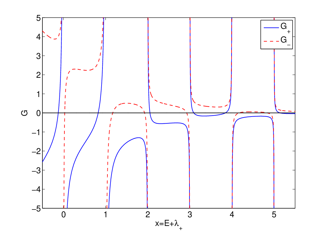
We plot the -function for in Fig. 1. The zeros reproduce all regular spectra, which can be confirmed by the numerical exact solutions. The energy spectra for and are presented in Fig. 2.
Exceptional solutions: We link the degenerate states to the Juddian solutions [28]. Koc et al. [29] have obtained isolated exact solutions in the isotropic QRM, which are just the Juddian solutions with doubly degenerate eigenvalues. The degenerate eigenstates are excluded in principle in the solutions based on the proportionality of Eq. (10) used in the present ECS technique. It naturally follows that the Juddian solutions are exceptional ones. With the -function (12) at hand, we can also discuss the Juddian solution [28] readily. The -function is also not analytic in but has simple poles at For special values of model parameters , there are eigenvalues which do not correspond to zeros of Eq. (12); these are the exceptional solutions. All exceptional eigenvalues are given by the positions of the poles
| (13) |
The necessary and sufficient condition for the occurrence of the eigenvalue is immediately given by
| (14) |
which provides a constraint on the model parameters. They occur when the pole of at is lifted because its numerator in Eq. (7) vanishes. Note that this exceptional eigenvalue belongs to the states with both even and odd parities, so it is doubly degenerate, and should be at the level crossing points without exceptions.


For
so we at most have one exceptional eigenvalue for at
| (15) |
It follows that the first excited state and the ground state only intersects for the CRW coupling weaker than RW coupling. The parity in the lowest energy state will change in this case, so the first-order quantum phase transitions occur at , in sharp contrast with the isotropic QRM. From Eq.(15), the first level crossing in Fig. 2 (left) should occur at , consistent with the numerical calculations.
For , the condition for the occurrence of the exceptional solutions is
| (16) |
If it reduces to
| (17) |
which is exactly the same as that in the isotropic QRM.
For high order exceptional solutions, the condition for the occurrence of the exceptional solutions is rather complicated, but can be numerically estimated straightforwardly from Eq.(14) . All of them are at the level crossing points with open circles in Fig. 2. Finally by the iteration in Eq. (7) , we can formally write the condition for the -th exceptional solution in terms of all coefficient
| (18) |
where is only model parameters dependent.
IV Generalized Rotating-Wave Approximation
To facilitate the approximately analytical study, we use a unitary transformation
Two displaced bosonic operators with opposite displacements, different from those in Sec. III, are introduced
The number state for the bosonic particles and are
| (23) |
then the Hamiltonian can be expressed with the number operators of the particles and
| (24) |
The wavefunction can be expressed as the following series expansion using these ECS
| (25) |
where stands for even (odd) parity, and is the truncated number of particles and .
Projecting onto the Schrdinger equation gives
| (26) |
where
| (27) |
where
Note that for , for , and if or . Here is the Laguerre polynomial. Eq. (26) can be reduced to that in the isotropic QRM [31] if set . Next, we will perform the approximation step by step.
Adiabatic approximations: if , i.e. the zero-order approximation, the eigenfunctions for the quantum number are give by ()
| (28) |
and the corresponding eigenvalues are
| (29) |
Similar to the isotropic QRM [31], the zero-order approximation in this technique is just the adiabatic approximations. It is also the same as the adiabatic approximation in Ref. [23] derived in an alternative way. Note that in the adiabatic approximations, the transition between states belonging to different manifolds is neglected.
Generalized Rotating-Wave Approximations: Beyond the adiabatic approximation, the transition between different manifolds should be considered. We will perform a further correction by taking into account the transition between states belonging to two manifolds and . The solutions for main quantum number can be obtained by selecting two terms in Eq. (26) for each and . Considering for the implied parity, we have the following determinant in a -by- block starting with
where . So we readily obtain the eigenenergies for each as
| (30) |
Note that for isotropic QRM, it is exactly the same as the GRWA result derived in Ref. [13, 12] in the isotropic QRM. So the present first-order approximation is also termed as the GRWA.
The lowest energy with even parity is
| (31) | |||||


For a given anisotropic parameters and , by Eqs. (30) and Eq. (31), we calculate the energy levels against both in the GRWA and the adiabatic approximation, which are presented in Fig. 3. The exact ones from the Sec. III are also presented for comparison. Obviously, the GRWA results agree well with the exact ones qualitatively in the whole coupling regime. The crossing properties are all present in the GRWA. The results by the adiabatic approximation obviously deviate from the exact ones and become worse with increasing and decreasing . The reason is that the transitions between states belonging to different manifolds in the true physical process are neglected in the adiabatic approximation, but the dominate transition from the manifolds and are taken into account in the GRWA. From the energy spectra, the difference between these two approximations is not very large, but they are essentially different. If the wavefunction is involved in some physical process, the difference should be remarkable. Further corrections to the GRWA will only result in qualitatively different results, and will not considered here.
Due to the counter-rotating wave terms, the eigenfunctions and eigenvalues of the anisotropic QRM present an open problem because they are not known in anything like a closed form, even the exact solutions reported recently[22] and the present new -functions. No analytical explicit expressions for the exact eigenvalues for the whole coupling range are available in the literature, to the best of our knowledge. The analytical explicit expressions presented in this paper might be practically useful.
V Conclusions
In this work, we first derive a concise -function, resembling to the compact one in the isotropic model, for the anisotropic QRM by using ECS, then obtain quite accurate approximate analytical solutions by another ECS. Zeros of the -function will yield the regular spectra. The isolated exact solutions are given by the exceptional solutions to this -function. The condition for their occurrence are also derived in the closed form. The crossing points of the energy levels satisfy this condition, similar to the single-mode QRM. The present analytic solution is well defined mathematically, because of no built-in truncations, thereby allowing a conceptually clear, practically feasible treatment to energy spectra and many physical processes. The explicit expressions for the eigensolutions in the GRWA are also obtained analytically by the another ECS. In a wide coupling regime, the GRWA results are very close to the exact ones.
Interestingly, this work adds the anisotropic QRM to a list with a compact -function like
| (32) |
where is determined recursively from . For the isotropic QRM with one-photon [18], . For the isotropic QRM with two-photons [19], , is given by Eqs. (48) and (49) there. For two-mode QRM [32], and is given by Eq. (28) there. In the present model, is dependent on model parameters and presents for all and . The qubit-cavity model possessing a compact -function like Eq. (32) shares the common property. The denominator of the parity dependent term, i.e. the second term in Eq. (32), is , so the zeros of its numerator will yield the condition for the occurrence of the exceptional solutions: isolated doubly degenerate eigenstates with eigenenergy , which is very helpful to analyze the structure of the energy spectra. This list may be expanded by absorbing other related models in the future.
ACKNOWLEDGEMENTS: This work was supported by National Natural Science Foundation of China under Grant No. 11174254.
∗ Corresponding author. Email:qhchen@zju.edu.cn
References
References
- [1] I. I. Rabi, Phys. Rev. 49, 324 (1936); 51, 652 (1937).
- [2] M. O. Scully and M. S. Zubairy, Quantum Optics (Cambridge University Press, Cambridge, 1997); M. Orszag, Quantum Optics Including Noise Reduction, Trapped Ions, Quantum Trajectories, and Decoherence (Science Publishing Group, New York, 2007).
- [3] A. Wallraff et al., Nature (London) 431, 162 (2004).
- [4] F. Deppe et al., Nature Physics 4, 686 (2008).
- [5] J. Fink et al., Nature 454, 315 (2008).
- [6] T. Niemczyk et al., Nature Physics 6, 772 (2010).
- [7] P. Forn-Díaz et al., Phys. Rev. Lett. 105, 237001 (2010).
- [8] A. Fedorov et al., Phys. Rev. Lett. 105, 060503 (2010).
- [9] J. Casanova et al., Phys. Rev. Lett. 105, 263603 (2010);
- [10] J. Hausinger and M. Grifoni, Phys. Rev. A80, 062320(2010).
- [11] S. He et al., Phys. Rev. A 86, 033837 (2012); ibid 90, 053848 (2014).
- [12] I. D. Feranchuk, L. I. Komarov, and A. P. Ulyanenkov, J. Phys. A: Math. Gen. 29 4035 (1996).
- [13] E. K. Irish, Phys. Rev. Lett. 99, 173601 (2007).
- [14] C. J. Gan and H. Zheng, Eur. Phys. J. D 59, 473 (2010).
- [15] F. Beaudoin, J. M. Gambetta, and A. Blais, Phys. Rev. A 84, 043832 (2011).
- [16] S. Swain, J. Phys. A 6, 1919 (1973).
- [17] Q. H. Chen, T. Liu, Y. Y. Zhang, and K. L. Wang, Europhys. Lett. 96, 14003 (2011).
- [18] D. Braak, Phys. Rev. Lett. 107, 100401 (2011).
- [19] Q. H Chen, C. Wang, S. He, T. Liu, and K. L. Wang, Phys. Rev. A 86, 023822(2012).
- [20] K. Furuya, M. C. Nemes, and G. Q. Pellegrino, Phys. Rev. Lett. 80, 5524(1998)
- [21] Y. X. Yu, J. Ye, and W. M. Liu, Scientific Reports 3, 3476(2013).
- [22] Q. T. Xie, S. Cui, J. P. Cao, L. Amico, and H. Fan, Phys. Rev. X 4, 021046 (2014).
- [23] M. Tomka, O. E. Araby, M. Pletyukhov, and V. Gritsev, Phys. Rev. A90, 063839 (2014).
- [24] S. I. Erlingsson, J. C. Egues, and D. Loss, Phys. Rev. B 82, 155456 (2010).
- [25] M. Schiroa, M. Bordyuh, B. Otu ztop, and H. E. Tureci, Phys. Rev. Lett. 109, 053601 (2012).
- [26] A. L. Grimsmo and S. Parkins, Phys. Rev. A 87, 033814 (2013).
- [27] Q. H. Chen, Y. Y. Zhang, T. Liu, and K. L. Wang, Phys. Rev. A 78, 051801(R) (2008).
- [28] B. R. Judd, J. Phys. C 12, 1685 (1979).
- [29] R. Koc, M. Koca, and H. H. Tütüncüler, J. Phys. A: Math. Gen. 35, 9425(2002).
- [30] C. Emary and E. F. Bishop, J. Math. Phys. (N.Y.) 43, 3916 (2002).
- [31] Q. H. Chen, L. Li, T. Liu, and K. L. Wang, Chin. Phys. Lett. 29, 014208 (2012).
- [32] Q. H. Chen, arXiv: 1412.8560 (2014).