Relaxation dynamics in a transient network fluid with competing gel and glass phases

We now characterize the dynamical properties of the system by focusing on two quantities: (i) the mean squared displacement, defined as $\Delta^{2}(t)=\langle\frac{1}{N}\sum_{i}\left\langle|{\bf r}_{i}(t)-{\bf r}_{i}(0)|^{2}\right\rangle$ and (ii) the self-intermediate scattering function, defined as $F_{s}(q,t)=\langle\frac{1}{N}\sum_{j}\exp\left(i{\bf q}\cdot[{\bf r}_{j}(t)-{\bf r}_{j}(0)]\right)\rangle$. Here ${\bf r}_{i}(t)$ is the position of particle $i$ at time $t$, $q$ is the wave-vector, and $\langle.\rangle$ corresponds to the ensemble average.

For increasing volume fraction $\phi=0.50,0.61,0.70$, we discuss simultaneously the data for $\Delta^{2}(t)$, shown in Fig. 3, and $F_{s}(q,t)$, shown in Fig. 4, computed at a wave-vector value $q=6$. Thus, the measured $F_{s}(q,t)$ probes the relaxation dynamics on length scales that are slightly larger than the average particle diameter (the peak in the structure factor $S(q)$ occurs at $q\approx{7.3}$).

We start in the pure gel phase ($\phi=0.50$). The mean squared displacement, Fig. 3a, shows that the increasing number of bonds restricts the motion of the particles in that for $R>0$ we see the emergence of an intermediate regime which develops into a well-defined plateau at $R=10$. The height of this plateau depends significantly on $R$, showing that this cage motion is directly related to the transient bonds between the particles. The self intermediate scattering function, Fig. 4a, shows for small $R$ a very rapid decay. This changes in that for $R$ around 4-6 a plateau develops at intermediate and long times, the height of which depends strongly on $R$. The presence of this increasing plateau height, which is reminiscent to the so called type-A transition of mode-coupling theory [33], indicates that the relaxation mechanism is changing: For small $R$ the motion of the particles is only weakly slowed down by the presence of the bonds, which typically break on the time scale of $\tau_{\rm link}$. However, for larger $R$ breaking a few bonds is not enough to allow the particles to move since the remaining bond still allow to maintain the particle inside its cage. Hence this makes that at large $R$ the relaxation dynamics does not depend very strongly on $R$ anymore. This effect is seen in Fig. 5 where we show the diffusion constant of the particles, $D$, (as obtained from the mean squared displacement at long times) as a function of $R$. For small $R$, $D$ shows a rather strong $R-$dependence, whereas for $R>5$ this dependence becomes weaker. Below we will discuss the $R-$dependence of the relaxation time in more detail.

Next, we look at the data for an intermediate density, viz. $\phi=0.61$, and in Fig. 3b we show the corresponding $\Delta^{2}(t)$. Like for $\phi=0.50$, the longtime diffusion decreases with increasing $R$, and the $R-$dependence of the diffusion constant shows again a break at around $R\approx 5$ (see Fig. 5). For this value of $\phi$ we observe, however, for $R>2$, at intermediate times a shoulder in $\Delta^{2}(t)$. This shoulder, clearly visible for $R=4$, is related to the presence of the bonds that lead to a caging of the particles on the length scale related to $\ell$, the maximum extension of a bond. Thus the hint of the short-time plateau (when $\Delta^{2}(t)\approx{0.1}$) and again one at later time (when $\Delta^{2}(t)\approx 1$) reflects the presence of the two different mechanisms for constraining particle motion, viz. local steric hindrance and the network bonds. Since each type of caging leads to a plateau in the intermediate scattering function [20], the existence of the two competing mechanisms makes that at intermediate times $F_{s}(q,t)$, shown in Fig. 4b, has a very slow, almost logarithmic, decay, if $R$ is around 6. More details on this particular case are give in the context of Fig. 11. If one compares the data for $R=10$ at the two volume fractions $\phi=0.50$ and $\phi=0.61$, we recognize that the height of the plateaus in $F_{s}(q,t)$ increases with $\phi$ from which one can conclude that the proximity of the particles leads to increased tightening of the cage.

If the density is increased further to $\phi=0.70$, the relaxation dynamics becomes strongly dominated by the steric hindrance mechanism. Already for $R=0$ one sees a weak plateau in $\Delta^{2}(t)$ and its length grows rapidly with increasing $R$ without changing much its height (see Fig.3c). This is the typical behavior of simple glass-forming liquids [44]. At the same time the self intermediate scattering function shows the growth of a shoulder with finite height and this height depends again only weakly on $R$, Fig. 4c. In contrast to the case at lower densities, here the shape of the correlator is basically independent of $R$. This is demonstrated in the inset of Fig. 4c where we plot $F_{s}(q,t)$ as a function of $t/\tau$, with the relaxation time $\tau$ defined by $F_{s}(q,\tau)=0.03$. The fact that this presentation of the curves leads to a nice master curve shows that we have for this system a time-$R$ superposition, in analogy to the time-temperature superposition found in simple glass-forming systems [1].

Despite the qualitative changes seen in $\Delta^{2}(t)$ and $F_{s}(q,t)$ if $\phi$ is increased, the $R-$dependence of the diffusion constant for $\phi=0.70$ is very similar to the one seen at lower densities, see Fig. 5. Also for this high value of $\phi$ we see that this dependence is relatively strong at small $R$ and becomes weaker if $R>6$. Hence the fact that at low $R$ just few bonds have to be broken in order to allow a particle to move whereas at high $R$ this is not a sufficient condition, is reflected in the $R-$dependence of $D$ at all $\phi$.

We will now explore further the interplay between the two processes leading to slow relaxation, i.e. the nearest-neighbor caging and the constrained motions due to the polymer bonds. Since the relative importance of these two processes depends on the lifetime of the polymer bonds, we will in the following vary this lifetime and consider values of $\tau_{\rm link}=10,10^{2}$, and $10^{3}$, and at fixed state-point of $R=6.3,\phi=0.61$, where logarithmic decay in the time-correlation function is observed. We study how the shape of $F_{s}(q,t)$ changes with varying $\tau_{\rm link}$ and will relate this to the interplay between the two processes. This is done for different values of wave-vector in order to see the how relaxation timescales vary over different lengthscales.

We begin by looking at the case of the large $\tau_{\rm link}=10^{3}$, i.e. when the polymer bonds hinder the motion on a time scale longer than the steric hindrance effect, see Fig. 6a. The correlation function reflects three different relaxation processes which can be seen for all value of $q$. Initially, the particles rattle inside the cage, resulting in partial relaxation of the correlation function on a timescale $\tau_{\beta}\approx 1$. Later on, the particles escapes from the cage of neighboring particles, (which for this value of $\phi$ not very pronounced), but the relaxation process is then held up by the polymer bonds. Eventually, the polymer network rewires on a timescale which is proportional to $\tau_{\rm link}=10^{3}$ and the particles start the final relaxation process. The height of the plateau in $F_{s}(q,t)$ increases with decreasing $q$, which is the typical behavior for a glassy system [44, 45]. However, for the range of wave-vectors explored, the final timescale for decay of $F_{s}(q,t)$ depends only weakly on $q$. Thus, over these length scales, the relaxation process is determined by the reconfiguration of the network. However, at larger length scales, one can expect that hydrodynamic effects will eventually dominate and this will then determine the relaxation timescales.

For intermediate values of the bond lifetime, $\tau_{\rm link}=10^{2}$ in Fig. 6b, the final decay has moved to shorter times and makes that now the interplay between the two processes results in a logarithmic decay of $F_{s}(q,t)$ as discussed elsewhere [20]. This logarithmic dependence is seen for a range of $q$ values (see Fig. 6b), with the time-window over which it exists decreasing with decreasing $q$. This implies that this form for the correlation function occurs only for specific combination of the relaxation timescales of the two processes of steric hindrance and eventual network relaxation. At sufficiently small $q$, hydrodynamics makes that the relaxation becomes so slow that the second relaxation step is no longer visible out and hence the logarithmic $t-$dependence is no longer observed. Finally we mention that the logarithmic shape in the relaxation function as discussed here is not related to any underlying higher order mode-coupling transition, in contrast to the case of certain colloidal systems for which similar relaxation functions have been observed [27].

If we set $\tau_{\rm link}$ to a small value, this three-step relaxation can no longer be observed, as is seen for the case of $\tau_{\rm link}=10$ in the bottom panel of Fig. 6: For all $q$’s the curve show a (seemingly) simple two step relaxation, since the third step (related to the bonds) starts already when the second step (related to steric hindrance) is not yet completed and hence the two processes become completely mixed in time. Below we will briefly come back to this effect.

A useful way to check the influence of the polymer bonds on the relaxation dynamics is by comparing the relaxation functions for the case when the bonds are permanent, i.e. $\tau_{\rm link}=\infty$, to those when the lifetime is finite. In Fig. 7, we do this comparison for different connectivities ($R=4,6,$ and 8) and different values of $\phi$.

In Fig. 7a, we show $F_{s}(q=6,t)$ for the case of $R=4$ with the two different bond lifetimes $\tau_{\rm link}=10^{2}$ and $\tau_{\rm link}=\infty$. For $\phi=0.50,$ 0.60, and 0.65, the timescales for overcoming the steric hindrance are the same for both lifetimes. However, for all $\phi$, we find that the correlation function for $\tau_{\rm link}=\infty$ shows a plateau at long times (not visible in this plot), which is due to the fact that the frozen bonds in the percolating gel-network prevent the complete relaxation of the system. In contrast the curves for the finite $\tau_{\rm link}$ vanish at long times. For small and intermediate $\phi$ the two sets of curves are very similar, indicating that the presence of a few bonds does not change the dynamics significantly. Only for $\phi=0.7$ one sees a substantial difference in that the correlator for the permanent links decays slower than the one with $\tau_{\rm link}=10^{2}$. It is reasonable that these differences are noticeable for times somewhat longer than $10^{2}$, i.e. the time scale of $\tau_{\rm link}$.

If we increase the connectivity to $R=6$ (Fig. 7b), we see that the behavior is qualitatively similar to $R=4$ in that for all values of $\phi$ the two curves track each other up to times around $10^{2}$, i.e. the time of the finite $\tau_{\rm link}$. For larger times the correlators for $\tau_{\rm link}=10^{2}$ decay to zero whereas the ones for $\tau_{\rm link}=\infty$ show at long times a marked plateau. The height of this plateau depends now more strongly on $\phi$ than it was the case for $R=4$, showing that if $R$ is increased the life time of the bonds becomes more influential. This is reasonable since it is related to the general observation that in glass-forming system small changes influence the relaxation dynamics increasingly more the slower the dynamics is. We also note that for $\phi=0.70$ the correlator for the permanent bonds becomes very stretched. This sluggish relaxation might be related to the fact that for this value of $R$ there are, in addition to the percolating cluster, clusters of different sizes (see Ref. [19] for typical distributions), thus giving rise to relaxation dynamics that spans many orders of magnitude in time and hence to a very stretched average correlation function. The stretching of the correlator for the frozen bonds could, however, also be due to the fact that these different clusters hinder each other resulting in the overall slowdown of the dynamics [46].

Next, we increase the number of bonds even more, viz. $R=8$, as shown in Fig. 7c. We see that for the case of permanent bonds the height of the asymptotic plateau has increased strongly in comparison to the case of $R=6$. As a result the correlator for $\phi=0.70$ shows only a negligible decay of the correlation function if the bonds are permanent. The motion is so constrained by these bonds that the height of the asymptotic plateau, caused by the permanent bonds, becomes comparable to the one related to the steric hindrance. Also for $\phi=0.5$ the height of the second plateau has increased so much that the relaxation from caging is now completely masked. However, for the intermediate values of $\phi$, one does notice a difference between the two plateau heights and the correlations functions decay in a very stretched fashion from one to the other. In fact, the decay is so slow that the time-dependence is seen to be logarithmic (nearly for five decades in the case of $\phi=0.65$). Note that this logarithmic decay is due to the heterogeneous relaxation of the floppy clusters of frozen bonds, which we will discuss later in further detail. Thus this mechanism is different from the one leading to the logarithmic relaxation seen in Fig. 4 which was due to a unique combination of the two finite relaxation timescales.

We now study the floppiness of this network of particles connected by the permanent bonds by probing the wave-vector dependence of the relaxation functions $F_{s}(q,t)$. In Figs. 8a and b, we show for $\phi=0.60$ the variation of $F_{s}(q,t)$ for $R=2$ and 4, i.e. in the region of the phase diagram where gelation sets in. The height of the plateau at long times, also called non-ergodicity parameter, is a measure for the stiffness of the network on the length scale $q$ considered. Comparing the two panels we recognize that, for a given $q$, the height of the plateau increases with increasing $R$. Denoting this height by $f_{q}^{\rm PN}$, we show in Fig. 8c that $f_{q}^{\rm PN}$ shows basically an exponential decrease in $q$ with a slope that decreases rapidly with increasing $R$. That $f_{q}^{\rm PN}$ decreases with increasing $q$ is of course reasonable since on small length scales the particles have more leeway to flop around than on large length scales. Note, however, that this exponential dependence is in contrast to the one found for the height of the plateau due to the steric hindrance, the latter being basically a gaussian function [45]. Since in the representation of Fig. 8c such a gaussian dependence is given by a parabola, we see that such a curve will intersect the one for $f_{q}^{\rm PN}$ at a certain value of $q_{x}$. For $q<q_{x}$ the plateau due to the steric hindrance is above $f_{q}^{\rm PN}$, thus making that one observes two plateaus in the correlator. However, for $q>q_{x}$ the plateau at long times is higher than the steric one, thus making that the latter one will be completely masked by the former and thus the correlator will show only one plateau.

We have also studied how the $q-$dependence of $f_{q}^{\rm PN}$ changes with the volume fraction and in Figs. 8d and e, we show $f_{q}^{\rm PN}$ for $R=4$ and 6, respectively. For both cases we see that the rigidity of the network at large scales, i.e. small $q$, is not affected by the volume fraction which is not surprising. For $R=4$ we see that this is also true at small length scales whereas for $R=6$ we note a significant $\phi-$dependence if $q$ is large. This difference is likely related to the fact that the system with $R=6$ is much more sluggish than the one for $R=4$, see Fig.7, and hence small changes (here in $\phi$) will have a stronger impact on the dynamics.

Finally we disentangle the dynamics of the particles that belong to the percolating cluster from the one that are not attached to it. In the following discussion these are referred as clustered and non-clustered particles, respectively. The objective is to clarify the respective contributions to the different dynamical quantities that we have discussed above. We do this comparison for an increasing number of connections $R$ at a fixed (large) volume fraction of $\phi=0.65$. In Fig. 9, we show the data for $\Delta^{2}(t)$ and $F_{s}(q,t)$ for these two families of particles.

The mean squared displacement of the clustered particles shows after the ballistic regime at short times a shoulder that is related to the cage of the steric hindrance (Fig. 9a). This localization is, however, only temporary and is followed by a further increase of $\Delta^{2}(t)$. Only at longer times $\Delta^{2}(t)$ saturates at a height that depends on $R$. We note that the approach to this asymptotic height becomes increasingly slow with increasing $R$ and in fact for $R=8$ the time dependence is close to logarithmic and does not end within the time window of our simulation. This behavior is also seen in the self intermediate scattering function $F_{s}(q,t)$ (Fig. 9b). At short times the correlator decays quickly onto a plateau (not very pronounced) before the relaxation of the steric hindrance starts. For $R=4$ and 6, this process ends in that the correlator reaches the final plateau (which is given by $f_{q}^{\rm PN}$ discussed above). However, for $R=8$ the final decay is so slow, again compatible with a logarithmic time dependence, that we do not see the asymptotic behavior.

Finally we look at the motion of the non-clustered particles and compare it with the one for $R=0$. From Fig. 9a we recognize that at this volume fraction also these particles are slowed down by the cage effect in that one sees for all values of $R$ a shoulder in $\Delta^{2}(t)$ at time $t\approx 1$. For $R=0$ the $\Delta^{2}(t)$ shows then immediately the diffusive behavior, i.e. it is proportional to $t$. However, if $R$ is increased, the $t-$dependence of $\Delta^{2}(t)$ for the un-clustered particles follows first the one of the clustered particles. Only once the latter starts to reach the plateau discussed above, do the former cross over to the diffusive behavior. Hence we can conclude that before this crossover the relaxation dynamics of the two population of particles are strongly coupled. This result is reasonable because in order to move, the un-clustered particles have to explore the holes within the percolating cluster formed by the particles which are permanently linked.

Also the self intermediate scattering function of the non-clustered particles tracks the one of the clustered particles at short times (Fig. 9b). However, once the latter starts to show at long times a plateau that has a significant height, the two correlators differ strongly since the one for the non-clustered particles decays to zero at long times. From the graph we also see that for $R=8$ the correlator is extremely stretched and shows almost a logarithmic $t-$dependence. This very slow decay indicates that the mobile clusters can move around the percolating cluster only with great difficulty, a behavior that is similar to the relaxation dynamics of particles moving in random porous media [47, 48]. It is also interesting that for the highest $R$ the mean squared displacement shows for the last two decades in time a nice diffusive behavior, whereas $F_{s}(q,t)$ is far from having decayed to zero. This apparent contradiction is related to the fact that $\Delta^{2}(t)$ is dominated by the particles that move relatively fast (i.e. they are in the small clusters) whereas $F_{s}(q,t)$ is dominated by the slowly moving particles (i.e. the large clusters). This cluster-size dependent dynamics leads to a so-called dynamical heterogeneity and in Section VI we will discuss this phenomenon in more detail.

Although we show in Fig. 9 the comparison between the dynamics of clustered and non-clustered particles for the case that $\tau_{\rm link}$ is infinitely large, it is evident that for a very large but finite value of $\tau_{\rm link}$ the relaxation dynamics will be very similar. Hence if, e.g., $\tau_{\rm link}$ is on the order of $10^{5}$, basically none of the shown curves will change significantly and thus the conclusions drawn from Fig. 9 will be apply also for such value of $\tau_{\rm link}$.

We now investigate how the two different relaxation timescales, one due to breaking of local cages and the other due to the reconfiguration of the network-bonds, vary with the volume fraction $\phi$ and the connectivity $R$.

To start we consider the case of structural relaxation related to the steric hindrance. In order to avoid that this relaxation process is influenced by the one of the network, we consider the case in which the latter is completely suppressed, which can be achieved by choosing $\tau_{\rm link}=\infty$. In the following we will study the relaxation times associated with the intermediate scattering function for wave-vector $q=6$. As discussed above, this correlator shows at long times an asymptotic plateau the height of which, $f_{q}^{\rm PN}$, depends on $R$ and $\phi$. To take this into account we define the relaxation time $\tau_{\rm SH}$, to be the time at which $F_{s}(q,t)-f_{q}^{\rm PN}=0.03$. The evolution of $\tau_{\rm SH}$ with $\phi$ is shown in Fig. 10a, for different value of $R$.

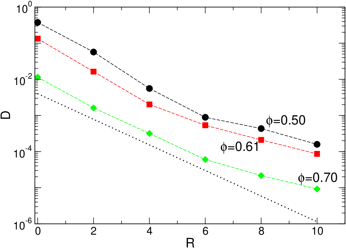
We see that in the absence of any bonds, i.e. for $R=0$, we have the usual slowing down of dynamics with increasing $\phi$. The $\phi-$dependence of the relaxation time can be fitted by a Vogel-Fulcher-Tammann-law of the form $\tau_{\rm SH}\sim{\exp[A/(\phi_{c}-\phi)^{\beta}]}$, with $\beta\approx 1$, from which we can estimate the volume fraction $\phi_{c}$ at which the relaxation times would diverge. If we increase the number of bonds among the particles, we see that $\tau_{\rm SH}$ increases. That this increase is not just a constant ($R-$dependent) factor but depends also on $\phi$ is demonstrated in the inset of the figure where we have normalized the relaxation times to its value at $\phi=0.5$. Using the Vogel-Fulcher-Tammann-law we can thus extract from these data the $R-$dependence of $\phi_{c}$, which can be considered as a proxy for the $R-$dependence of the glass transition temperature. This $\phi_{c}(R)$ line is included in Fig. 1 as well and we see that it has a weak negative slope with $\phi_{c}(R=0)=0.847$ and $\phi_{c}(R=6)=0.808$. Thus we can conclude that the glass transition as induced by the steric hindrance mechanism does not depend strongly on the value of $R$. However, since the prefactor of the Vogel-Fulcher-law does depend strongly on $R$, we can conclude that a line of iso-relaxation time will bend significantly more.

Next, we investigate how the timescale for the full relaxation of the network of particles depends on the average number of bonds, $R$. For this we define a relaxation time using the $t-$dependence of $F_{s}(q=6,t)$ with a very short lifetime for the bonds ($\tau_{\rm link}=1$). $\tau_{\rm PN}$ is then defined via $F_{s}(q=6,\tau_{\rm PN})=0.03$ and the $R-$dependence of this relaxation time is shown in Fig. 10b. The figure shows that for small and intermediate values of $R$ the $R$-dependence is independent of the volume fraction in that the curves for the different values of $\phi$ seem to be just shifted vertically. That this is indeed the case is demonstrated in the inset where we show that a plot of the same data, but now normalized to the relaxation time for $R=0$, gives a master curve. The main panel shows that at small concentration of bonds the $R-$dependence is close to an exponential, a result that is likely related to the fact that increasing $R$ leads to a tighter cage for the steric hindrance and hence a slower dynamics. However, for intermediate values of $R$ the curve $\tau_{\rm PN}$ start to bend over towards a weaker $R-$dependence. In order to investigate this effect better we have carried out simulations for $\phi=0.50$ at very high values of $R$: 16, 30, and 50. We find that in this regime the relaxation time follows closely an exponential (see main Fig. 10b), but with an exponential scale that is smaller than the one seen at small $R$. Note that this dependence implies that there is no singularity in the relaxation dynamics at any finite value of $R$, at least for this volume fraction. Instead the dynamics shows a behavior that is similar to an Arrhenius law in that the barrier for the relaxation depends only on the number of bonds between the particles. This observation is in agreement with earlier simulations for equilibrium gels [51].

We conclude this discussion by using the different relaxation timescales to develop a criterion that tells whether or not the correlator $F_{s}(q,t)$ will show the logarithmic $t-$dependence discussed in the context of Fig. 4b. For this we define $f_{q}^{\alpha}$ as the height of the plateau associated to the $\alpha$-process, with $\alpha\in\{{\rm SH,PN}\}$, and recall that $\tau_{\beta}$, $\tau_{\rm SH}$ and $\tau_{\rm PN}\propto\tau_{\rm link}$ are the timescales for the three different relaxation processes described above, namely the rattling inside the cage, the escape from the local cage, and the network renewal process. We can now define a simple criterion for the anomalous logarithmic relaxation to be observed by requiring that the slope of the two segments defined by pairs $[(\ln\tau_{\beta},f_{q}^{\rm SH}),(\ln\tau_{\rm SH},f_{q}^{\rm PN})]$ and $[(\ln\tau_{\rm SH},f_{q}^{\rm PN}),(\ln\tau_{\rm PN},0)]$ is the same, see Fig. 11. It is known that for glass-forming systems the plateau related to steric hindrance is a Gaussian functions of the wave-vector $q$, $f_{q}^{\rm SH}\sim\exp(-q^{2}\ell_{\rm SH}^{2})$ [45]. We showed earlier, see Fig. 8c, that for the PN-process, $f_{q}^{\rm PN}$ has an exponential shape at large $q$ (the regime corresponding to anomalous logarithmic behavior). Putting these elements together we thus obtain

We begin by looking at how the non-Gaussian parameter varies with changing connectivities $R$, either when we go from the liquid to the gel phase, at $\phi=0.50$, or when we are in a strongly glassy region, $\phi=0.70$. For the case $\tau_{\rm link}=10^{2}$ the data is shown in Fig. 12.

For $\phi=0.50$, Fig. 12a, $\alpha_{2}(t)$ shows at $t\approx 1$ a peak if $R=0$ and a shoulder for $R>0$. This feature is thus related to the dynamical heterogeneity due to the steric hindrance mechanism, as in usual glass-forming systems [44]. For $R>0$ we find in addition a very prominent peak the location of which is basically independent of $R$, which shows that for this packing fraction the time at which the system is maximally heterogeneous does not depend on $R$. This observation is in tune with our earlier discussion that the timescale for structural relaxation at small values of $\phi$ does not change with $R$ if the number of bonds is not very large (see Fig. 4a). The maximum occurs around $t\approx{10^{3}}$, a time which corresponds to a timescale for which a significant number of particles have broken the bonds with their neighbors and exit the constraints of the network. The location of the peak is thus somewhat larger than $\tau_{\rm link}$. As has been documented in Ref. [17], at small packing fractions one has on this timescale two families of particles, one for the mobile particles and the other related to those that are immobile and as a consequence the shape of $G_{s}(r,t)$ deviates strongly from a Gaussian. Figure 12a indicates thus that the same behavior persists to the larger volume fraction of $0.50$. One interesting feature is that the peak height is non-monotonous in $R$ in that it increases till $R=6$ and then decreases again for larger $R$ values. The reason for the growth is that an increasing $R$ allows for more diverse values of the connectivity for the particles, and hence to a stronger variety in the dynamical behavior. On the other hand, if $R$ is very large most of the particles are strongly connected all the times and hence show a much smaller variation in their relaxation dynamics, i.e. they behave like in a mean-field like regime.

Next we study the behavior for $\phi=0.70$, Fig. 12b. When there are no bonds, $R=0$, we see that $\alpha_{2}(t)$ is peaked at around $t=8$. This peak, which is related to the steric hindrance, corresponds thus to the one seen for $\phi=0.50$ at $t\approx 1$ and which, due to the higher density has shifted to larger times. For $R=2$ (when the percolating cluster of the bonds develops), the location of this peak slightly shifts to larger times and one sees the appearance of a second peak at $t\approx 2000$ (corresponding to the timescales for renewal of the network connectivities). However, the dominant heterogeneity is still due to the local steric hindrances. As $R$ is increased, the location of the first peak continues to shift to longer timescales, in track with the increasing structural relaxation timescales (see Fig. 4c), and also its height increases, in qualitative agreement with the behavior found in simple glass-formers if the coupling is increased [44]. For $R=6$, the two peaks have merged, since the timescales for the two sources of heterogeneity are nearly the same, and thus $\alpha_{2}(t)$ has a single peak. If $R$ is increased even more, the position of the peak moves to larger times, but its height starts to decrease. The reason for this decrease is likely the same as the one we indicated when we discussed the data for $\phi=0.50$, i.e. that for large $R$ the system starts to become mean-field like and hence heterogeneities are suppressed.

We also note that the height of the peak is significantly smaller than the one for $\phi=0.50$. Thus, at large density, steric hindrance dominates and even the faster particles have less space to move around resulting in significantly less non-Gaussian shapes for $G_{s}(r,t)$. As a consequence, the dynamics is more homogeneous in this regime compared to the gel at lower $\phi$.

To elucidate the origin of the two peaks in the non-Gaussian parameter at $R=2,\phi=0.70$, we determine how the distribution of particle displacements $G_{s}(r,t)$ evolves with time. This is shown in Fig. 13. At short times, particle motion is restricted by the local cage of neighbors and thus $G_{s}(r,t)$ is a Gaussian at small $r$. At larger distances the distribution has an exponential tail which is due to a few particles that have escaped the steric hindrance cage, in agreement with the usual heterogeneous glassy dynamics in supercooled systems [4]. The presence of these two processes gives rise to the maximum in $\alpha_{2}$ at short times. At around $t=400$, most of the particles have escaped from this steric hindrance cage and thus the dynamics of the system becomes more homogeneous with $G_{s}(r,t)$ assuming a Gaussian form and hence $\alpha_{2}$ decreases again. But with time, the motion of the particles is again restricted, this time by the bonds which have not yet relaxed. Thus again $G_{s}(r,t)$ develops a Gaussian shape (with a larger width, determined by the length of the connecting bonds) and an exponential tail, implying an increase in $\alpha_{2}$. Later, the network eventually relaxes, the particles are diffusive and thus $\alpha_{2}$ decreases again.

The presence of these two different contributions to the shape of $\alpha_{2}(t)$ can be further clarified by varying the lifetime of the network, i.e. $\tau_{\rm link}$, and in Fig. 14 we show this for the case $\phi=0.65,R=6$. Since we scan a large span of timescales and $\alpha_{2}$ changes strongly, the data is shown in logarithmic scales. For $\tau_{\rm link}=1$, we see only a small peak at $t\approx 10$, which corresponds to the one due to the steric hindrance. For $\tau_{\rm link}=10^{2}$, we find that this peak has increased a bit in height and its location has also shifted to $t\approx 30$. This change is a consequence of the increased effective coupling between the particles due to the increased lifetime of the bonds. In addition, we see the development of a new (weak) peak at $t\approx{10^{3}}$, which is caused by the network renewal process. Now, if we increase $\tau_{\rm link}$ further, the location of the first peak remains at the same place, since the local crowding effects are unaffected by the network dynamics. In contrast to this, the location of the second peak shifts to longer timescales and its height increases strongly. Since the position of this peak scales with $\tau_{\rm link}$, we recognize that this peak is related to the renewal process. Finally, if we take the case of permanent bonds between the particles, the curve is nearly identical to that for $\tau_{\rm link}=10^{4}$, except that we see no signature of it eventually decreasing with time. The reason for this runaway effects is the fact that with increasing lifetime of the network, the unattached particles diffuse away and travel long distances before the network is again renewed. This results in very long extended tails in $G_{s}(r,t)$ which shows up as very large values for the non Gaussian parameter. For the case that $\tau_{\rm link}$ diverges the dynamics never becomes Gaussian and $\alpha_{2}(t)$ diverges at long times.

It is interesting that if one computes, for $\tau_{\rm link}=\infty$, $\alpha_{2}(t)$ separately for the clustered and non-clustered particles, only the peak at short times is observed, i.e. the one which is due to the crowding effects. This is shown in the Inset of Fig. 14 for the case of the system of particles where there is a permanently frozen percolating cluster and few unattached particles. In this case, the $\alpha_{2}(t)$ for the clustered particles follows the curve for the full system, shows the bump at short times and becomes at long times a constant (see the corresponding data for $\Delta^{2}(t)$ in Fig. 9). The result that at long times $\alpha_{2}(t)$ does not go to zero, as it would be the case for vibrations in a typical amorphous solid with $R=0$, is related to the fact that the spanning cluster is a disordered network of particles that have different local environments. Thus the large variety of slow floppy motions, related to the slow relaxation in $F_{s}(q,t)$ over long times (see Fig. 9), gives a non-Gaussian shape for $G_{s}(r,t)$ even at very long times. This non-Gaussianity is also the reason for the exponential shape of $f_{q}^{\rm PN}(q)$, as observed earlier, see Fig. 8. For the non-clustered particles, $\alpha_{2}(t)$ does show a slight decrease beyond the short-time maximum which shows that the relaxation dynamics starts to become a bit more homogeneous. However, it cannot be expected that the non-Gaussian parameter will go to zero even at very long times, since the mobile clusters do have a spread in size and hence a different diffusion constant.

We conclude by measuring to what extent the observed heterogeneous dynamics is related to a correlated motion of the particles. This can be quantified by $\chi_{4}(q,t)$, defined above, measured for $q=6.0$, i.e. we look for relaxations over distances which are slightly larger than the average particle diameter.

To have a reference we consider first the case $R=0$, i.e. when there are no polymers and the system is just a standard glass-forming system. The time dependence of $\chi_{4}(q,t)$ is shown in Fig. 15a for different packing fractions. In agreement with earlier studies on similar systems, Ref. [50], we find that $\chi_{4}(q,t)$ shows a maximum at a time $t$ that increases with $\phi$ and which tracks the increasing relaxation time $\tau_{\rm SH}$. The fact that the height of the peak increases with increasing $\phi$ indicates that the relaxation dynamics become more cooperative, also this in agreement with previous studies for other glass-forming systems [52].

Next, we contrast this behavior with the case of increasing gelation, i.e. we fix a volume fraction and increase the number of polymer bonds. For this, we choose $\phi=0.70$, i.e. the same packing fraction for which we have studied the correlation functions and the non-Gaussian parameter, since for this $\phi$ the effects due to the steric hindrance as well as the network constraints are clearly observed. The corresponding $\chi_{4}(q,t)$ is shown in Fig. 15b for $\tau_{\rm link}=10^{2}$. For $0<R\leq 6$, the location of the peak in $\chi_{4}(q,t)$ shifts to larger times and the height of the maximum increases. Thus this trend follows the behavior observed in the data for $F_{s}(q,t)$ as well as $\alpha_{2}(t)$, indicating that steric hindrance dominates the relaxation process and that the dynamics becomes more and more collective. However, for $R>6$, the peak height decreases again and its location becomes independent of $R$. We can thus conclude that in this regime the relaxation dynamics becomes less cooperative, a result that makes sense since the rewiring of the network is not really a collective process. This result is also in qualitative agreement with the decrease of the maximum in $\alpha_{2}(t)$, see Fig. 12b, which showed that the dynamics becomes more homogeneous.

We conclude by investigating how the lifetime of the network-bonds influences the function $\chi_{4}(q,t)$. For this we have calculated this observable for the case $\phi=0.65$ and $R=6$, i.e. at intermediate density and in the gel phase for which one sees a significant $\tau_{\rm link}$-dependence in the relaxation behavior (see Fig. 7b). We see, Fig. 15c, that at small and intermediate $\tau_{\rm link}$ the location of the peak in $\chi_{4}(q,t)$ moves to larger time and that its height increases somewhat, i.e. a behavior that is directly related to the steric hindrance mechanism in which the effective cage becomes stiffer due to the increased lifetime of the bonds. However, once $\tau_{\rm link}$ exceeds $10^{4}$, we see that $\chi_{4}(q,t)$ no longer depends on this lifetime, i.e. the rewiring of the network no longer affects the cooperativity of the dynamics and the latter is solely dependent on the steric hindrance.