From Field Theory to the Hydrodynamics of Relativistic Superfluids
A Dissertation Submitted to the Faculty of Physics at the
Vienna University of Technology
by
Stephan Stetina
Vienna, September 2014
Abstract
The hydrodynamic description of a superfluid is usually based on a two-fluid picture. In this thesis, basic properties of such a relativistic two-fluid system are derived from the underlying microscopic physics of a complex scalar quantum field theory. To obtain analytic results of all non-dissipative hydrodynamic quantities in terms of field theoretic variables, calculations are first carried out in a low-temperature and weak-coupling approximation. In a second step, the 2-particle-irreducible formalism is applied: This formalism allows for a numerical evaluation of the hydrodynamic parameters for all temperatures below the critical temperature. In addition, a system of two coupled superfluids is studied. As an application, the velocities of first and second sound in the presence of a superflow are calculated. The results show that first (second) sound evolves from a density (temperature) wave at low temperatures to a temperature (density) wave at high temperatures. This role reversal is investigated for ultra-relativistic and near-nonrelativistic systems for zero and nonzero superflow. The studies carried out in this thesis are of a very general nature as one does not have to specify the system for which the microscopic field theory is an effective description. As a particular example, superfluidity in dense quark and nuclear matter in compact stars are discussed.
Dedicated to my parents with deep and profound gratitude. I would not be the person I am today without their constant support and guidance.
Preface
Superfluidity is a very general phenomenon. Critical temperatures of known superfluids extend over 17 orders of magnitude (from about 200 nK for cold atomic gases to up to K for nuclear and quark matter). In the frame of this thesis, I will be most interested in the upper end of this scale and discuss relativistic superfluids which presumably exist in dense nuclear or quark matter in the interior of compact stars. Due to its interdisciplinarity, the study of this field is as fascinating as it is challenging. Concepts of many different branches such as particle physics, solid state physics or astrophysics have to be taken into account and I will devote a rather large part of this thesis to describe the rich spectrum of physics to which the research presented in this thesis is relevant.
The basic idea is to relate the effective hydrodynamic description of a superfluid to the underlying microscopic theory. The relevant microscopic physics are determined by a relativistic quantum field theory to which a Bose-Einstein condensate is introduced. Even though it is to some extent obvious that the hydrodynamics of a superfluid evolve from such a microscopic background, this relation has never been made explicit before. The existence of such a “gap” in our perception of superfluidity has led the existence of two separate communities (a “phenomenological” and a “microscopic” one), each equipped with a terminology of its own. This difference in terminology is a frequent source of confusion and I hope the results of this work can help to eliminate at least some of this confusion. In the second part of this thesis, I shall demonstrate explicitly that it is indeed possible to the derive the hydrodynamic description and calculate all non-dissipative hydrodynamic parameters purely in terms of field theoretic variables. It shall also be indicated how the obtained results are related to recent research outside of high energy physics, in particular to liquid helium and cold atoms. In the third part I will use this microscopic framework to study the sound excitations of a superfluid. In part IV, the more complicated but phenomenologically important scenario of two coupled superfluids will be discussed.
Most of the results were obtained in a collaboration with my thesis advisor Andreas Schmitt11 1 Univ.Ass. Dr. Andreas Schmitt, Institute for Theoretical Physic, Technical University Vienna andreas.schmitt@tuwien.ac.at as well as Mark Alford 22 2 Prof. Mark G. Alford, Physics Department, Washington University of St. Louis, alford@wuphys.wustl.edu and Kumar Mallavarapu 33 3 S. Kumar Mallavarapu, Physics Department, Washington University of St. Louis, kumar.s@go.wustl.edu from the Washington University in St. Louis. In particular the results presented in sections 8 and 10,11 and 12-15 of this thesis were published in the following two articles
- •
M. G. Alford, S. K. Mallavarapu, A. Schmitt, S. Stetina, Phys. Rev. D 87, 065001 (2013)
- •
M. G. Alford, S. K. Mallavarapu, A. Schmitt, S. Stetina, Phys.Rev. D89, 085005 (2014)
Acknowledgments
I would like to use this opportunity to express my deepest gratitude towards my thesis advisor Andreas Schmitt. Over the past years, I have come to value him not only as an excellent and dedicated teacher, but also as a great mentor. In addition to uncountable discussions in frame of the research projects we carried out together, his counseling in academic affairs in general and in preparation of conference talks or writing scientific articles in particular have been invaluable to me. I find it hard to believe that the quality of my PhD training could have been any better.
I would also like to thank Anton Rebhan for many valuable comments and suggestions and in particular for granting me additional financial support.
I thank Mark Alford, Karl Landsteiner and Eduardo Fraga for inspiring and valuable discussions.
Finally I would like to thank the Austrian Science Fund FWF for the financial support I have received over the past three years.
Part I Introduction
The discovery of superfluidity originated from the study of the low-temperature dynamics of helium. Helium exhibits the rather peculiar feature of remaining liquid - even when the limit of absolute zero temperature is approached. While we are not aiming to describe the properties of helium as accurately as possible, no introduction to superfluidity can be complete without mentioning some of the spectacular experimental results of these studies. Most of the discussed properties are not exclusive for helium but are properties of superfluids in general. In particular, we shall explain how the theoretical attempts to describe the observed phenomena ultimately led to the powerful two-fluid formalism which will be introduced in section 2. A relativistic version of this two-fluid formalism is widely and successfully used today to describe the phenomenology of superfluids in compact stars (see also section 5). After a short historical outline of the discovery of compact stars we will discuss the properties of matter which presumably exists in compact stars from a microscopic point of view. In particular, we shall explain in which phases of dense matter we expect to encounter superfluidity and how the occurrence of superfluidity influences observable phenomena of compact stars. The microscopic terminology used in section 4 will inevitably be very different from the phenomenological one used in sections 1 and 2. It shall be the goal of second part of this thesis to make the relationship between both approaches as explicit as possible. A review of the discovery of superfluidity containing many interesting historical details can be found in [1]. In addition, reference [2] provides a good introduction to the phenomenology of superfluidity.
1 Early experiments with liquid helium
The experimental discovery of superfluidity dates back to the year 1927 when Keesom, Wolfke and Clusius discovered an anomaly in the properties of liquid 4He 44 4 This is by far the most abundant isotope of helium and used in most laboratory experiments. Each pair of neutrons, protons and electrons occupies a 1s orbital, none of them possesses orbital angular momentum and the spin of each pair adds up to zero. In this configuration, helium is extremely stable. : the specific heat as a function of temperature shows a sharp maximum at 2.17 K [3, 4]. According to the shape of this diagram this point was called “lambda point” and marks the boundary of two different liquid states referred to as helium I (above ) and helium II (below ). Shortly after the discovery of this novel He II phase, experimental efforts focused on the study of heat-flow and viscosity of helium II which seemed to show a rather unusual behavior:
Rollin in Oxford realized [7] that the heat transport in Helium II is up to 5 times as effective as in Helium I and shows a sharp peak at a temperature around 2 K (a typical plot is shown in 1.1).
It was conjectured that convection (due to the bulk motion of the fluid as opposed to heat conduction due to excitations of molecules) could be responsible for the anomalously large value of heat transport provided that the viscosity is small enough. However, the usual convection law (i.e. a linear relation between heat-flow and temperature gradient where denotes the thermal conductivity) was only recovered for sufficiently small temperature gradients. In addition, Brewer and Edwards measured the thermal resistance as function of the heat flow [6]. This relation remains constant up to a critical value of the heat flux at which the thermal resistance suddenly increases rapidly (see right panel of figure 1.1). This critical value of the heat flow corresponds precisely to the critical value of the temperature gradient at which nonlinear deviations from the convection law become measurable which suggests a deeper connection between both phenomena. In fact, both can be explained by the concept of a critical velocity: as we will discuss in the paragraph below, a heat flux induces a counter-flow of mass flux (and vice versa). The mass flow however is limited by a certain critical velocity at which turbulence arises (see discussion in section 6.1). This in turn is the origin of the sudden increase in thermal resistivity and for the onset of a nonlinear regime of the heat flow.
The counter-flow mechanism was discovered by two spectacular experiments which showed the so called “thermomechanical effect” and its inverse, the “fountain effect” [8]: in case of the thermomechanical effect, two containers were filled with helium II and connected by a very thin capillary - a so called “superleak” which should be thin enough to block any viscous fluid. Increasing the pressure

in container A leads to a flow of helium towards container B. Surprisingly, this induces a temperature difference in both containers: while the temperature increases in A, it decreases in B. This shows that mass flow and heat flow are not just interconnected, but even pointed in opposite directions. The fountain effect was discovered, when a flask (open at the bottom) with a thin neck was lowered into a bath of helium II. Additionally, the lower part of the flask is filled with a fine compact powder - again with the purpose of preventing any viscous liquid from escaping through the bottom. As soon as the helium in the flask is heated up, a fountain of liquid helium sprays out at the top. Such a process can in principle go on as long as the heat supply as well as the cooling of the bath are provided.
The absence of viscosity in helium II was shown in 1938 independently by two groups, Kapitza [10] in Moscow and Allen and Misener [11] in Cambridge by measuring the flow velocity of helium through thin capillaries. The published articles of both groups include remarkable statements about the nature of superfluidity: Kapitza proposed [10] that “by analogy with superconductors […] helium below the point enters a special state which might be called superfluid”. This is the first time the term superfluidity appears in literature. Furthermore, superfluidity is related to superconductivity long before the microscopic theory of the latter phenomenon was established. Kapitza received the Nobel price for his discovery in 1978. Allen and Misener on the other hand claimed [11] that “the observed type of flow[…] cannot be treated as laminar or even as ordinary turbulent flow”. This statement implied that helium II requires an entirely new fluid-dynamical description and was in contradiction to the common view of that time that liquid helium is an “ordinary” fluid with very small viscosity (i.e. an ideal fluid describable by Euler‘s equations of motion).
The pioneers in setting up this entirely new theory of fluidity were Fritz London and Laszlo Tisza. London argued [12] that since 4He atoms were Bose particles, they should undergo Bose-Einstein condensation, a rather new concept at that time. He then calculated the transition temperature of an ideal Bose gas with the density of liquid 4He and arrived at a value of 3.1 K, quite close to . London also explained, why Helium II remains liquid when the temperature approaches absolute zero: even at very low pressure, the quantum kinetic energy of helium atoms is large compared to their binding energies due to Van der Waals forces. In addition, helium atoms are particularly light. As a net result, helium atoms do not remain “frozen” at fixed lattice positions even at very low temperatures. Shortly after Tisza learned about London’s ideas, he proposed a two-fluid model [13] consisting of a superfluid that would have zero entropy and viscosity and a viscous normal fluid which carries entropy. With the aid of such a model he was able to provide an intriguingly simple explanation of the thermomechanical effect: heating in terms of the two fluids means converting superfluid into normal fluid at a rate sufficient to absorb the applied energy. Near the heater, this results in an excess of the normal fluid and a deficiency of the superfluid. Convection then leads to a counterflow of both components: while the superfluid is drawn towards the heater (where it will be transformed), the normal fluid flows away from the heater. Any temperature inhomogeneity in a superfluid is efficiently smoothened out by this counterflow mechanism. This effect is directly visible in experiments:

when pressure is reduced below vapor pressure, we expect that boiling of helium II sets in. Usually boiling becomes visible by the onset of bubbles, which represent local hot spots in a liquid. However, in boiling helium II one cannot observe any bubbles55 5 Once again, this effect is limited by the critical velocity. If the induced counterflow becomes too large an onset of bubbles is indeed visible. .
In case of the two containers which are connected by a small capillary, only the superfluid can pass (the viscosity of the normal fluid prevents it from creating a counterflow through the narrow capillary such that no equilibrium between the two containers can be achieved). This situation is illustrated in figure 1.3. Since there is now more mass (but the same entropy!) in container B, the temperature decreases. By the same argument, the temperature increases in container A. From the same experiment, it was deduced that the charge is carried by the superflow: a steady state (when there is no more flow through the superleak) is only achieved when the chemical potentials are equal in both containers . According to the thermodynamic relation, a pressure gradient corresponds to gradients in temperature and chemical potential , but only a gradient in the chemical potential will induce a superflow. Tisza was also able to explain the fountain experiment: heating creates a temperature difference between the helium within the flask and the helium bath below causing the superfluid to enter the flask. The viscous normal fluid on the other hand is prevented from leaving the flask due to the powder at the bottom. The volume of the liquid in the flask thus increases rapidly resulting in a fountain shooting out at the top.
Finally it was Landau, who perfect the two-fluid model. At this point, it is interesting to mention that Landau, despite his certainly outstanding intuition refused to believe in the relevance of Bose-Einstein condensation. Nevertheless, Landau‘s theory is a remarkable success. The main advance compared to Tisza‘s model lies in the definition of the normal component. While Tisza believed that the normal fluid consists of uncondensed atoms, Landau proposed that it is made of quasiparticles of the quantum fluid. In a manner of speaking, both Landau and Tisza were correct about a different half of the two-fluid model. Landau divided all quasiparticle excitations into two groups which he termed “phonons” and “rotons”. While the “phonon” has a dispersion relation linear in momentum and determines the low-temperature properties of the fluid, the “roton” dispersion is quadratic in momentum and can only be excited after a certain energy gap has been reached66 6 The microscopic nature of the roton excitations is still heavily debated today. Different microscopic models aim to reproduce the roton spectrum with different levels of success.. After fitting model parameters such as to reproduce the experimental value of the specific heat, he calculates a transition temperature of about 2.3 K in very good agreement with the experimental value.
Perhaps the most striking prediction of the two-fluid model is the existence of an additional sound mode: Landau proposed that heat should propagate as what he calls “second sound” rather than diffuse as in an ordinary fluid. Even though the idea of temperature waves also originated from Tisza, the results differed in both models: Landau predicted that second sound approaches a value of with being the velocity of ordinary sound waves in the zero temperature limit while in Tisza‘s model the velocity of second sound approaches zero. The experimental confirmation of Landau‘s result ultimately marked the success of his model which we shall briefly review in the next section.
2 The two-fluid model
Landau essentially constructed his famous two-fluid model based on the experimental results reviewed in the last section. We will now discuss the non-dissipative version of this model, i.e. we will consider a mixture of a superfluid and an ideal fluid (the normal component). A generalization which takes into account the viscosity of the normal fluid is discussed for example in [14]. The basic equations of motion of an ideal fluid are built on the fact that the motion of a fluid within a given volume element can be described by the mass density , the entropy density and the fluid velocity . The corresponding equations read:
| (2.1) | |||||
| (2.2) | |||||
| (2.3) |
Equivalently to the Euler equation the conservation of momentum can be used
| (2.4) |
where the momentum density is given by and the stress tensor of an ideal fluid by
| (2.5) |
These equations can be solved for , and provided that the equation of state is supplemented.
To explain the experimental fact that entropy does not flow with the center mass velocity , it is obviously necessary to go beyond the Euler set of equations and introduce an independent velocity field associated with the entropy flow. This velocity is denoted by , reflecting that only the normal fluid carries entropy. The velocity of the superfluid on the other hand is constrained by the condition that no turbulence occurs (at least not for flow velocities below the critical velocity). In mathematical terms, the superfluid velocity is assumed to be irrotational, . The mass density is divided into superfluid and normal-fluid density77 7 It should be noted that this is merely an interpretation, the two densities cannot be physically separated. It is not possible to determine which helium atoms belong to the normal fluid and which to the superfluid. where the normal-fluid density vanishes at zero temperature and the superfluid density at the critical temperature. By definition, the two fluid components interpenetrate each other without mutual friction. The total mass flow adds up to:
| (2.6) |
The conservation of mass remains unchanged
| (2.7) |
whereas the conservation of entropy is now given by
| (2.8) |
Momentum conservation can be written in the form of (2.4) using equation (2.6) and the stress tensor of the two-fluid system
| (2.9) |
It remains to find the corresponding Euler equation for the superfluid. As demonstrated by Khalatnikov [14], this equation can in principle be derived from conservation equations postulated above, the irrotationality of the superflow and the principle of Galilean invariance (see also reference [15]). However, such a derivation is tedious and we shall follow Landau‘s original approach: in order to explain why the chemical potentials on both sides of a superleak are equal in the steady state Landau postulated that the chemical potential acts as the potential energy of the superfluid component and as the corresponding force. The superfluid Euler equation then reads
| (2.10) |
Equations (2.7, 2.5) and momentum conservation form a complete set of eight independent hydrodynamic equations describing the motion of a superfluid in terms of the eight variables , , and provided that the equations of state , and are supplemented. Galilean invariance requires the equations of state to depend only on the difference of and and to be invariant under rotations. A few concluding remarks about the two fluid equations are in order:
- •
In the strict mathematical derivation of the two-fluid equations, frame dependence plays an important role. While in the single fluid case, one can always define a local rest frame of the fluid, this is no longer possible in the two-fluid case. In the way listed above, the two-fluid equations are obviously given in a lab frame where and are both nonzero. When we consider relativistic superfluids, the Galilean transformation connecting two frames of reference will have to be replaced by a Lorentz transformation. Especially when deriving the corresponding hydrodynamic equations from microscopic physics, frame dependence will be a non-trivial issue.
- •
The irrotationality condition of the superfluid implies that the superflow can be expressed as the gradient of a scalar potential . When terms quadratic in the velocities are neglected, equation (2.10) turns into . This is an important relation indicating that velocity and chemical potential of a superfluid can be obtained as time and spatial derivatives of the same scalar field . The relation follows after taking the time derivative
(2.11) In a relativistic context, it seems natural to unite chemical potential and superflow using the four gradient . In a microscopic context, we will later identify the field as the phase of a Bose-Einstein condensate.
- •
The two-fluid framework can be extended to include dissipation. The equation of motion for the normal component is then to be replaced by a Navier-Stokes equation. In the simplest case, linear deviations from equilibrium in the hydrodynamic parameters are considered. While the conservation equations of mass and momentum can be extended to include dissipative terms, entropy is no longer conserved. One rather has:
(2.12) Here, denotes the dissipative entropy flux and is a positive definite quantity (the positive entropy production due to dissipation will drive the system back into equilibrium after some time). These assumption result in a modified Navier-Stokes equation which is rather complicated (an explicit expression can be found in [14]). The two-fluid Navier-Stokes equation differs from the regular one in the number of viscosity coefficients: in addition to the shear viscosity, three bulk viscosity coefficients rather than one are present. It should be noted that the concept of two fluid components which interpenetrate each other without mutual friction becomes problematic in the presence of dissipation. A detailed discussion of the validity of the two-fluid picture including viscosity can be found in [15].
3 The discovery of compact stars
The discovery of Sirius B by Walter Adams in 1915 is regarded as the first discovery of a compact star. Using stellar spectroscopy, he was able to deduce [16] that despite of its size which is roughly about the size of the earth, Sirius B had a mass that is comparable to that of the sun. In reference to their hot temperature and small size, such objects were called “white dwarfs”. Due to the high densities present in a white dwarf, atoms are fully ionized, all electrons are free and form a degenerate gas. It was soon realized that relativistic effects are important for a realistic description of such an electron gas [17].
In February 1932, James Chadwick discovered the neutron [18] after only two weeks of experimentation. It is often mentioned in literature that this discovery served as a motivation for Landau to speculate about the existence of neutron stars. This however seems not to be the case (see reference [19] for a historical review). The submission of Landau‘s first publication on compact stars [20] dates back to January 1932 - one month before Chadwick‘s discovery. While it is true that Landau predicted the existence of stars with the structure of “gigantic atomic nuclei”, he was obviously unaware of the existence of neutrons at that time as he describes the atomic nucleus as being made of protons only (Landau would not consider neutrons for another six years). The first model of a nucleus made of protons and neutrons was suggested by Ivanenko in April 1932 [21].
The term neutron star was first introduced in 1933 by Walter Baade an Fritz Zwicky [22] at Caltech in an attempt to explain the enormous amount of energy released in supernova explosions (the gravitational collapse of the core of a massive star). As they correctly explained, such a supernova explosion represents the transition of an ordinary star into a neutron star - an object made up of closely packed neutrons with a very small radius and extremely high density. In 1939, George Gamov realized [23] that white dwarfs are analogous to neutron stars: both represent the final evolutionary state of a star, but a white dwarf is the supernova remnant of a star whose mass was not large enough to become a neutron star (which is the case for over 97% of the stars in our galaxy). However, the existence of neutron stars remained controversial. In 1939, Robert Oppenheimer and George Volkov found analytic solutions to the Einstein equations of general relativity for the special case of static and spherical stars made of isotropic matter. Based on the resulting equation (also called Tolman-Oppenheimer-Volkov equation), they calculated an upper limit for the mass of neutron star to roughly 0.7 solar masses [24] - smaller than the mass of stellar cores that could collapse into neutron stars. The crucial ingredient is the equation of state: while Oppenheimer and Volkov used an equation of state for a degenerate non-interacting neutron gas, a similar calculation based on Skyrme-model effective nucleon interactions resulted in a maximum mass as high as two times the solar mass [25] and general interest in neutron stars raised again.

In the meantime a consistent microscopic theory of Cooper pairing was established and possible applications in nuclear matter where studied by Nicolay Bogolyubov in 1958 [26]. Only one year later, Arkady Midgal suggested that superfluidity might be present in neutron stars - a first study was carried out by Vitaly Ginzburg and David Kirzhnits in 1964 [27]. Since then, a great number of possible phases of matter (including superfluid ones) in compact stars that go beyond ordinary nuclear matter have been suggested and we will review some of them in the next chapter. It was not until 1967 that the first direct observation of a neutron star finally took place. Jocelyn Bell Burnell and Antony Hewish measured radio emissions originating from a fast rotating neutron star, a so called pulsar [28], located in the “crab-nebular” - a remnant of a gigantic supernova bright enough to be directly observed by Chinese astronomers in 1054. Hewish was awarded the Nobel price for this discovery in 1974.
4 Compact stars from a microscopic point of view
In the frame of this thesis, we will reserve the word compact star for objects which are dense enough to support nuclear and/or deconfined quark matter in their inner layers. The physics of white dwarfs mentioned in the last chapter will not be considered here. Nucleons and quarks are strongly interacting particles and therefore, the dynamics of matter inside a compact star are mainly determined by quantum chromodynamics (QCD). However, electroweak interactions induce further constraints on the composition of matter. To describe dense matter in compact stars, we first need to discuss the phase diagram of QCD and clarify where in this diagram compact stars exist. Since we are ultimately interested in superfluidity (i.e. a low-temperature phenomenon), we shall discuss in which sense matter inside a compact star can be considered as cold. In order to review superfluidity in dense and strongly interacting matter, we will make use of a modern microscopic picture, in which superfluidity is the result of spontaneous symmetry breaking. We will not elaborate further why a system subject to spontaneous symmetry breaking exhibits superfluidity at this point as this will be discussed in great detail in part II. The impact of superfluidity on the phenomenology of a compact star will be explained in section 4.2.
4.1 Cold and dense nuclear and quark matter
In what follows, only three quark flavors (up, down and strange) will be considered. Quark chemical potentials in a compact star can reach values up to about 500 MeV - by far not enough to excite heavier quarks. (If not explicitly stated otherwise, the symbol will refer to the quark chemical potential.) The presence of electrons might be required in compact star matter to achieve electric neutrality and the corresponding chemical potential will be denoted as . If we were to consider purely strong interactions, we could assign a chemical potential to each separately conserved quark flavor. However, weak interactions violate flavor symmetries and we shall see that as a result the number of independent chemical potentials is reduced from four () to two ( and ). Despite the high densities of matter inside a compact star, the mean free path of neutrinos is still large enough to allow them to escape. Lepton number is thus not conserved and no chemical potential can be assigned to it. Finally, any cluster of matter is formally required to be a color singlet and thus there is no net chemical potential for color charges in a compact star (with the exception of non-uniform phases in which sub domains with positive and negative charge can in principle exist [29]). In the high energy limit, quark masses can be neglected and the overall symmetry group of QCD including color gauge group as well as left and right-handed flavor groups reads:
| (4.1) |
While the current quark masses of up and down quark of about 5 MeV are negligible, the strange quark mass of about 90 MeV will certainly have a strong impact on the composition of matter inside a compact star. The following features of QCD are particularly important for our understanding of the phase structure of strong interactions:
- •
QCD is an asymptotically free theory which means that the coupling strength between quarks decreases with increasing momentum transfer. At sufficiently high energies and/or densities, QCD thus behaves like a free field theory. This behavior can effectively be described by a running coupling where the characteristic energy scale is experimentally determined to a value of 200 MeV. Only when the momentum transfer is larger than this value, say above , perturbative calculations are valid.
- •
At sufficiently low temperatures and/or densities, quarks are confined into color-neutral composite particles (hadrons). Critical temperature and density of the deconfinement transition can vaguely be related to the characteristic energy scale: corresponds to a temperature of the order of K at which hadrons are melted into their constituent quarks. Furthermore, the size of a light hadron measures about 1 fm which roughly corresponds to . If the average separation distance of quarks is below 1 fm (at a chemical potential of around 400 MeV) deconfinement sets in. It should be noted that even though asymptotic freedom and confinement can at least vaguely be related to one energy scale , they should be treated as independent: while confinement is the dominant characteristic of the theory at low energies, asymptotic freedom becomes dominant at high energies.
- •
At low temperatures and densities, chiral symmetry (the symmetry of independent left and right handed flavor rotations) is spontaneously broken by a color-neutral quark/anti-quark condensate The resulting ground state is only invariant under simultaneous rotations of left and right handed quark flavors (i.e. vector rotations)88 8 The full symmetry group can be decomposed in vector and axial-vector symmetries which correspond to simultaneous () and opposite () rotations of left and right handed flavors. However, the symmetry is violated in any region of the phase diagram by quantum effects (axial anomaly) and reduced to the descrete group . We will surpress this residual group in the breaking patterns. The vector symmetry corresponds to baryon number conservation and will from now on be denoted as .
(4.2) The above pattern indicates that the axial symmetry is maximally broken resulting in Goldstone bosons - the pseudoscalar meson99 9 Pseudoscalar particles are characterized by zero total spin and odd parity, usually denoted as . octet. It should be noted that chirality is an approximate symmetry valid only at asymptotically high energies and its breaking is a complicated dynamical matter: instead of exactly massless Goldstone bosons one obtains pseudo-Goldstone modes with small masses.
For the sake of completeness, it should be mentioned that chiral symmetry breaking and confinement not necessarily share a common phase transition line and in principle a confined but chirally symmetric phase might exist. We will ignore this possibility here and project a crude first version of the phase diagram with a single phase boundary separating confined and deconfined quark matter in figure 4.1.
From these generic features of QCD, we can deduce that compact stars are located in an area of cold and dense matter in the QCD phase diagram: shortly after their creation in a supernova explosion, the temperature of compact stars is of the order of 10 MeV ( roughly ). During the evolution of a compact star, it further cools down to temperatures in the keV range which is small compared to scale set by . Chemical potentials of compact stars on the other hand can become as large as MeV. We are thus particularly interested in a region of and . At very high temperatures a plasma of asymptotically free quarks and gluons is realized. Entropy prohibits a well ordered ground state and there is no spontaneous symmetry breaking in this region of the phase diagram - in other words all symmetries of the group are effectively restored. Experimental data of the transition to this state matter can be obtained from relativistic heavy ion colliders. A powerful theoretical tool to probe this transition is lattice QCD which, at least in the vicinity of the temperature axis, predicts a smooth crossover from hadronic matter to quark-gluon plasma. In the limit of , a rich phase structure due to a large variety of symmetry breaking patterns is anticipated. Because of asymptotic freedom, it seems reasonable to begin a discussion of cold and dense quark matter at very high densities where properties of the ground state can be deduced from first principles (i.e. QCD) and then investigate what happens once we progress downwards in density.

4.1.1 Highest densities, Color flavor locking
A comprehensive introduction to the physics of high density quark matter can be found for example in references [29] and [30]. At asymptotically high densities, quark masses can be neglected and the quark Fermi momenta become large. Due to Pauli blocking, only states in the vicinity of the Fermi sphere are modified by interactions. Such interactions then involve large momentum transfer and are governed by weak coupling. As a result, we expect to find a Fermi liquid of weakly interacting quarks and quark-holes. However, in contrast to Coulomb forces acting between electrons, interactions between quarks are certainly attractive in some channel which can be deduced from the existence of baryons which are bound states of quarks. Such attractive interactions between quark quasi-particles will render the ground state unstable with respect to Cooper pairing1010 10 As discussed for example in [29], the energy scale at weak coupling below which the quasiparticle picture of quarks breaks down is parametrically of order while the BCS order parameter (the energy gap in the excitation spectrum of the quasiparticles) is parametrically larger of order . In other words, pairing occurs in a region of the phase diagram where the quasiparticle picture of the quarks and thus also the BCS argument remains rigorously valid. and these pairs, possessing bosonic quantum numbers, will undergo Bose Einstein condensation. This argument, as originally presented by Bardeen, Cooper and Schrieffer (BCS) [31] holds true for quarks in quark matter in the same way as it does for electrons in a solid1111 11 In some sense, the pairing mechanism is even simpler in quark matter as an attractive interaction in QCD is directly provided by single gluon exchange (which is the dominant process at weak coupling) whereas in a solid, a complicated framework of electron - phonon interactions is required. . So far, we can make two important observations on high density quark matter:
- •
The ground state of high density quark matter spontaneously breaks baryon conservation, and therefore is a baryon superfluid. Since baryon conservation is an exact symmetry of QCD for any given density, the spontaneous breaking of is also the origin of superfluidity in nuclear matter.
- •
Since the order parameter of Cooper pairing is a di-fermion condensate , it cannot be a color singlet but rather breaks the symmetry. Thus, quark matter at highest densities is not only a superfluid but also a color superconductor.
It remains to determine the structure of the BCS order parameter in color, flavor and spin space. Interactions between quarks can be decomposed into a symmetric sextet as well as an antisymmetric anti-triplet channel:
| (4.3) |
This holds true for color as well as flavor degrees of freedom. In color space, quarks must be in the anti-triplet representation as this channel provides attractive interactions while interactions in the sextet channel are repulsive. Since pairing is preferred in the antisymmetric spin zero channel and the overall wave function of a Cooper pair has to be antisymmetric, we can conclude that quarks pair in an anti-triplet flavor channel. The color and flavor structure of the Cooper pair is thus given by:
| (4.4) |
Expanding in an antisymmetric color and flavor basis, we can write:
| (4.5) |
The matrix now determines the specific color and flavor structure of the Cooper pair within the antisymmetric basis. To maximize the condensation energy, quarks of all colors and flavors are required to contribute to the Cooper pairing. This allows for an unique determination of the order parameter and one obtains [32]. This diquark order parameter breaks the symmetry group down to simultaneous rotations of color and flavor degrees of freedom:
| (4.6) |
and related to this breaking pattern, the corresponding ground state has been termed color-flavor locking (CFL) [32]. The breaking of baryon conservation to the discrete subgroup reflects the cooper pair nature of the ground state. To complete the discussion of CFL, we list all elementary excitations of this phase:
- •
The spontaneous breaking of baryon conservation gives rise to a discrete massless Goldstone mode as well as a gapped mode with a finite spectral weight [33]. We shall see that the Goldstone mode is crucial in the discussion of superfluidity, the massive mode becomes relevant only at higher energies.
- •
CFL breaks chiral symmetry as can be seen in the breaking pattern (4.6). The low energy spectrum of CFL hence contains 8 light (pseudo)-Goldstone modes with quantum numbers identical to those of the meson octet resulting from chiral symmetry breaking in low-density QCD (4.1). The corresponding excitations can therefore be considered to be the high density analogues of pions, kaons and the particle1212 12 At this point, it is interesting to mention that the symmetry properties of CFL and hadronic matter in principle allow for the intriguing possibility of a quark-hadron continuity, see references [34], [35] and [36]. . The meson octet is complemented by a singlet state resulting from the breaking of . Due to the axial anomaly, the particle mass becomes large at lower densities whereas at large densities, the effect of the anomaly becomes arbitrarily small (see also discussion in section 4.1.2). The (pseudo) Goldstone modes together with the (exact) Goldstone mode resulting from the breaking of determine the dynamics of CFL at low energies .
- •
The (pseudo) Goldstone modes in CFL are accompanied by nine gapped excitations (i.e. the quark-quasiparticles) where one of them has a gap of magnitude and the remaining eight of magnitude [30].
- •
The color gauge group is completely broken resulting in Meissner masses for all glouns. The generator of the electromagnetic charge on the other hand is contained in the flavor group 1313 13 This is visible for example in the covariant derivative. To couple electric charges to the three quark flavors, the charge generator -1/3) is coupled to the electron chemical potential . and due to symmetry breaking in CFL, only the residual generator remains unbroken. In other words, all diquark condensates carry zero net -charge. This phenomenon is called rotated electromagnetism. is a linear combination of the generator of the original electromagnetic charge and the gluon generator and the new gauge field reads . However, since the mixing angle is very small, one may say that the (original) photon does not acquire a Meissner mass and CFL is not an electromagnetic superconductor.
A phase diagram including the CFL phase is shown in figure 4.2. In summary, the properties of the CFL phase at highest densities allow for a rigorous theoretical treatment from first principles: QCD is weakly coupled at high densities and infrared divergences are are cut off by the Meissner masses of the gluons. Furthermore, magnetic interactions in QCD are screened by Landau damping [29].
It remains to provide a quantitative estimate in which density regime one can expect CFL to represent the ground state. Calculations of the order parameter of CFL in the frame of BCS theory are reliable at a chemical potential of the order of about MeV1414 14 It should be emphasized that this magnitude of the chemical potential specifically describes the limit at which the BCS gap equation is valid. It should not be confused with a threshold at which perturbative calculations become applicable - the gap equation is derived under the assumption of weak coupling, but it is still non perturbative. [37] (roughly 15 orders of magnitude larger than the maximum value for chemical potentials inside compact stars). Parametrically, one obtains the following result [38]:
| (4.7) |
This shows that the gap in CFL is parametrically larger than the standard BCS result for the gap which is proportional to . This deviation results from the fact that the point like four-fermion interaction has been replaced with the long-range gluon interaction. As increases faster than decreases [29], one can conclude that the gap increases for asymptotically large . The critical temperature of CFL deviates by a factor of from the standard BCS result
| (4.8) |
As in standard BCS theory, the critical temperature is of the same order of magnitude as the zero temperature gap. With these results at hand, it is tempting to try a bold extrapolation to densities existing inside compact stars. According to the QCD beta function, a chemical potential of about 400 MeV corresponds to a coupling of (of course we can only rely on the two loop approximation of the beta function which strictly speaking is not valid at all at lower densities). This results in a gap (and thus also in a critical temperature) of the order of 10 MeV - above temperatures of a compact star except for the first minutes after their creation. Even though such an extrapolation seems of course unreliable, a comparison with models specifically designed to describe an intermediate density region such as the NJL (Nambo Jona Lasinio) model shows surprisingly good qualitative agreement [39]. This suggests that color superconductors are at least strong candidates for the ground state of matter inside a compact star. What really happens to the ground state of QCD once we leave the save grounds of asymptotically high densities is very hard to determine as our current theoretical control over the region of intermediate densities is very limited. Some insights can be obtained by extrapolations from nuclear theory (upwards in density) or, as we will discuss in the next section, from CFL (downwards in density). Another possibility is to use effective models for this region of the phase diagram. More powerful and reliable methods such as lattice QCD or experimental insights from heavy ion collisions are limited to lower densities (one should not however, that future accelerator facilities such as NICA might provide some insight [40] and also in lattice QCD some progress in the effort to extend calculations to higher densities has been made [41]). From this point of view, the study of compact stars as the only “laboratory” where such intermediate densities are realized in nature could prove to be invaluable.

4.1.2 High, but not asymptotically high densities
Two effects become important once we leave the realm of asymptotically high densities:
- •
The coupling strength increases. This effect renders calculations from first principles outside the asymptotic density region very complicated and it is very challenging to include higher order effects in the coupling constant. Approaches to resolve this issue include the construction of an effective field theory for quasi-quarks and gluons near the Fermi surface [42] or renormalization group theory [43]. In the effective field theory approach, strong coupling makes it necessary to include non Fermi liquid effects at energy scales above the gap [44], [45].
- •
The mass of the strange quark increases and the Fermi momentum decreases. The separation of the Fermi momenta of different quark flavors eventually leads to the breakdown of Cooper pairing1515 15 For two fermion species with chemical potentials and , a first order transition to the unpaired phase sets in at , the so called Chandrasekhar-Clogston point. . To obtain a quantitative estimate, when this happens for 3-flavor CFL, one has to take into account that matter inside a compact star is constrained by charge neutrality and beta equilibrium1616 16 In quark matter, decay and electron capture are represented by , and , respectively and an additional non-leptonic process is given by . These constrain the chemical potentials to and (as stated before, there is no chemical potential for neutrinos). , which couples the chemical potentials. In unpaired quark matter, the lack of negative electric charge due to the reduced number of strange quarks (charge ) is compensated by lowering the up-quark (charge ) Fermi momentum and increasing the down-quark (charge) Fermi momentum (the electron contribution to the charge density is parametrically negligibly compared to the quark contributions, for a more detailed discussion see [30]) resulting in the ordering . To leading order in one finds an equidistant separation of between all quark flavors. In CFL quark matter, the pairing locks the Fermi momenta together as long as the energy cost of enforcing the pairing is compensated by the energy released from the condensation of Cooper pairs. As the cost of maintaining a common Fermi surface is parametrically and the gain of condensation energy is , we can expect paired quark matter to remain stable as long as . It should be noted that such a limit is not exclusive to the pairing pattern of CFL: less symmetric pairing patterns which might appear as increases (for example patterns in which only two flavors contribute to the pairing) suffer the same fate of stressed pairing [46]. From these simple estimates, it is of course not possible to decide, whether CFL is robust enough to extend all the way down to the phase boundary of nuclear matter or not.
Systematic studies show that as long as densities are still high enough and the stress on the pairing pattern is not too large, CFL will most likely react with the development of a kaon condensate [47]. To understand why kaon condensation is particularly important in this context, we will take a closer look at the effective theory for mesons in CFL first derived in reference [44]. The construction of this effective theory works analogously to chiral perturbation theory in nuclear matter: the chiral group is assumed to be intact which is an appropriate approximation as long as quark masses are small compared to the specific scale of chiral symmetry breaking. This scale is set by the high density analogue of the pion decay constant which was calculated [48] to
| (4.9) |
It should be noted that in contrast to the chiral effective theory in vacuum, the finite chemical potential in the high density effective theory explicitly breaks Lorentz invariance (see also discussion in section 5.3). The meson fields appear to all orders in the chiral field ,
| (4.10) |
where are the Gellmann matrices. contains an octet of mesons under the unbroken symmetry. The subscripts and now correspond to the charges which are attributed in the same way as (regular) electric charges are attributed to vacuum mesons. There is however an important difference to vacuum mesons: the Cooper pair nature of the ground state in CFL leads to mesons which are given by a condensate rather than by quark/anti-quark bound states. This can be deduced from the fact that quark flavors in CFL are paired in the anti-triplet representation, see (4.4). Replacing quarks with anti-quarks (and vice versa) while preserving their flavor quantum numbers results in the identification or . In order to reproduce the flavor quantum number of, say, a neutral kaon, one then has to replace with . Obviously, as the quark content of the “CFL-mesons” differs from the vacuum mesons, so will their mass ordering.
Since the effect of the axial anomaly becomes arbitrarily small at high densities, the overall symmetry group under of the effective theory is given by . The chiral field and mass matrix transform under chiral rotations as and . The somewhat peculiar transformation property of is related to the explicit breaking of chiral symmetry induced by finite quark masses: in order to recover a chirally symmetric theory, it is necessary to require that the mass matrix is not passive under chiral transformations but transforms as . Under transformations, the chiral field transforms as . Once again, to enforce invariance under axial transformations, is required to transform as . Collecting all possible mass contributions up to the second order, the effective Lagrangian for mesons in CFL reads
| (4.11) |
where and the constant can be obtained from weak-coupling calculations. Remember that the mesons fields are contained in the exponent of and are thus present to any order. It can be shown [47] that and act as effective chemical potentials for right-handed and left-handed fields. The corresponding symmetry group can formally be treated as a gauge symmetry, which allows us to introduce a covariant derivative . The corresponding mass terms then enter the theory in the usual way of a chemical potential as the zeroth component of the covariant derivative:
| (4.12) |
If we where only to consider the symmetry, these terms would cover all possible mass contributions. Due to the additional requirement of invariance, also the second term in proportional to is allowed up to second order in (for more details on the construction of mass terms see also [49]). Terms linear in are in principle forbidden by the symmetry group of as they break the axial symmetry . In vacuum chiral perturbation theory where the effect of the axial anomaly is strong, a linear term of the form is included instead of the invariant term proportional to in (4.11). Weak-coupling results in the high density regime for and indeed show that is suppressed for large and the term proportional to is dominant while at lower densities the situation is reversed.
Diagonalization of the mass terms of (4.11) leads to the result that the mass ordering of mesons in CFL is reversed1717 17 In particular, the meson which is the Goldstone boson corresponding to breaking is now the lightest meson since the effect of the anomaly is suppressed. as compared to vacuum mesons [49] . This is one of the reasons why in CFL kaon condensation is favored over pion condensation. It is worth emphasizing that this effective theory is constructed on symmetry properties only. If the scaling of the CFL gap and the quark masses with the chemical potential were known, the effective theory would be applicable far outside the weak-coupling regime and represent a powerful tool to calculate properties of matter inside a compact star.
To study kaon condensation, we can set all meson fields except the neutral kaons in the exponent of to zero and denote the fields in which correspond to the neutral kaons by the complex field . Then we separate the vacuum expectation value from fluctuations
and expand up to fourth order in the fields[50]:
| (4.13) |
As a result, one obtains a complex scalar theory. We shall use such a theory as a starting point for the derivation of superfluid hydrodynamics in part II. For the current discussion we can neglect fluctuations and consider only the potential:
| (4.14) |
where the effective mass, chemical potential and coupling are obtained in terms of the parameters of the high density effective theory as:
| (4.15) |
The mass depends on the coefficient which in turn is proportional to . A similar derivation of the effective neutral pion mass results in which is indeed larger than the kaon mass. From these results it becomes obvious why CFL with (neutral) kaon condensation (CFL-) is a reasonable candidate to succeed (pure) CFL once we progress downwards in density. We have seen that the stress induced by a finite strange quark mass on unpaired quark matter in equilibrium is compensated by converting strange quarks into mostly down quarks. In CFL matter where all quasi-quarks are gapped, the system rather counteracts the lack of strangeness with the population of mesons that contain down quarks and strange holes (i.e. kaons). Bose-Einstein condensation of these particles will occur if the effective chemical potential becomes larger than the effective mass. Since and , the condensation of neutral kaons is likely to occur in a region of decreasing and increasing and . Similar arguments also apply to positively charged kaons . However, the positive charge requires the presence of electrons to achieve electric neutrality which disfavors a condensed phase. A calculation of the critical temperature of kaon condensation [50] extrapolated to densities of about MeV yields MeV. This is of the order of or even larger than the critical temperature of CFL. In other words, in a region of the phase diagram, where parameters are such that is guaranteed, CFL quark matter should develop a kaon condensate. Since the kaon condensate spontaneously breaks conservation of strangeness
we expect this phase to be a kaon superfluid. It should be noted that weak interactions violate the conservation of strangeness and is not an exact symmetry to begin with. However, this violation is relatively mild as the finite mass of the (pseudo) Goldstone boson of 50 keV [30] is small compared to the critical temperature of kaon condensation.
Given the rather exotic value of MeV at which CFL can be taken for granted, it is unknown whether this phase (with or without meson condensation) really extends all the way down to phase boundaries of nuclear matter. Other candidate ground states such as superconductors with two-flavor or single flavor pairings, Spin-1 superconductors or crystalline phases have been discussed in great detail in literature (see reference [29] for a review). As discussed in the end of section 4.1.1, the absence of reliable theoretical or experimental tools in this region of the phase diagram leaves us behind with a formidable challenge.

Finally, after crossing this unknown region we reach the hadronic phase which is relatively well describable by means of effective models which are - at least at sufficiently low densities - well constrained by nuclear scattering data. The hadronic phase is subdivided in a gaseous and a liquid phase at a chemical potential of MeV. The phase structure is summarized in figure 4.3. At higher densities and low temperatures, nuclear matter might be superfluid. In fact it is the spontaneous breaking of the same symmetry group that leads to superfluidity in dense nuclear matter as baryon number is always an exact symmetry in any density regime of the QCD phase diagram. Since we are now in the confined phase of QCD, we cannot deduce the properties of the ground state from first principles but have to rely on an effective microscopic description. The attractive interaction between protons and neutrons necessary for the formation of Cooper pairs can be described by the exchange of mesons instead of gluons1818 18 An appropriate model to describe such interactions is for example the Walecka model. In its simplest version, protons and neutrons interact via the exchange of the scalar and the vector meson (superfluidity in such a model is discussed for example in reference [51]). . In hadronic matter at low densities, protons and neutrons pair in the channel, where we have used the spectroscopic notation to specify total spin , angular momentum and total angular momentum . At higher densities, medium effects as well as three-body interactions of the nuclear forces become important and pairing most likely happens in the channel (see reference [52] for a recent review on pairing in nuclear matter).
Also meson condensation is considered in nuclear matter where again the focus lies on the condensation of (in this case negatively charged) kaons. condensation is motivated by the fact that medium effects in nuclear matter lead to an increase of the pion mass whereas the effective kaon mass is reduced (for a review of strangeness in neutron stars see reference [53]). Furthermore, as soon as densities are large enough for kaons to condense, it becomes favorable to create a new Fermi sphere for negatively charged kaons instead of adding additional electrons at large momenta in order to achieve electric neutrality. The conversion of electrons into kaons is subdivided into electron capture () followed by neutron decay () with the neutrinos escaping the star. As a net result, a large number of neutrons is converted into protons and matter becomes more and more isospin symmetric.
Hyperons are estimated to appear at densities of about two times nuclear saturation density1919 19 Nuclear saturation density is defined is the density of nucleons in an infinite volume at zero pressure. It should be emphasized that the term nuclear matter does not address matter inside a nucleus but rather an idealized state of matter of a huge number of neutrons and protons interacting via strong forces only. In the absence of external forces, the nucleons will then arrange themselves in a preferred density of (If for instance, nucleons are added to a very large nucleus, the density of the nucleons will remain approximately constant at the value of ). The corresponding binding energy per nucleon is . In a compact star, densities are typically as large as several times nuclear saturation density. [53] and depending on critical temperatures and densities, they might constitute additional superfluid components. In particular, the and particle are often considered in literature as they are conjectured to appear first with increasing density. It should be mentioned that the recent discovery of a two-solar-mass neutron star [54] challenges the hypothesis of hyperonic matter and/or meson condensation in neutron stars since the equation of state including hyperons seems to limit the maximum mass of a neutron star to lower values. This is all the more surprising since at a certain density threshold, the onset of hyperons seems unavoidable. This so called “hyperon puzzle” is currently among the most heavily debated issues in compact star physics.
In summary, one can see that superfluidity appears in many different spots and at various densities in cold strongly interacting matter :
- •
CFL is a fermionic superfluid since it spontaneously breaks baryon conservation . The scalar field theory analyzed in part II can be seen as a low-temperature approximation to such a system for energies smaller than the magnitude of the superconductive gap. Expected temperatures in the interior of compact stars suggest that this is a reasonable approximation.
- •
At high but not asymptotically high densities, systematic studies show that CFL will most likely develop a kaon condensate. The corresponding ground state is a bosonic superfluid since it spontaneously breaks conservation of strangeness . The effective theory for kaons in CFL (4.11) can even be more directly related to a complex scalar field theory as we have discussed above. However, it is still an approximation since explicit symmetry breaking effects due to weak interactions are neglected. It is important to realize that the spontaneous breaking of happens “on top” of the symmetry breaking pattern of CFL. A hydrodynamic description of CFL and kaon condensation is therefore highly non-trivial: in addition to two superfluid components (a quark and a kaon superfluid), a normal fluid is present. In part IV, we will discuss how such a coupled system of superfluids can effectively be described in terms of coupled scalar fields.
- •
Finally we encounter superfluidity in compact stars at much lower densities, where proton superconductivity and neutron superfluidity might coexist. Again, one might use an effective bosonic description to model the low-temperature dynamics. However, in order the describe proton superconductivity, the global symmetry would have to be replaced by a local gauge symmetry. If coexisting hyperon superfluidity is taken into account, one has to handle an even more complicated mixture of different fluid components (a mixture of nucleon-hyperon superfluids has for example been considered in [55]).
4.2 Phenomenology of compact stars
We have seen that nuclear or quark matter at intermediate densities is notoriously hard to tackle and the study of compact stars perhaps the only available way to gain further insights. Naturally, the question arises whether the microscopic composition of matter inside a compact star can be related to macroscopic effects observable to astrophysicists. This could lead to a fruitful symbiosis: a profound understanding of dense matter from first principles allows for a more precise modeling of compact stars whereas on the other hand observations of compact stars can help to constrain microscopic models. Superfluidity, being a macroscopic quantum phenomenon, is certainly of great interest in this respect.
To the best of current knowledge, a compact star can be subdivided into 3 different regions [56], see figure 4.4; Atmosphere, crust, and core. Nuclear and quark matter are most likely limited to the core with a radius of several kilometers which in turn is subdivided into inner and outer core: in the outer core, densities can reach up to two times and matter is most likely composed of a large fraction of neutrons accompanied by a small admixture of protons as well as electrons and possibly muons constrained by the condition of electric neutrality. While electrons and muons presumably form an ideal Fermi liquid, neutrons and protons constitute a strongly interacting Fermi liquid and are most likely in a superfluid (superconducting) state. In the inner core of a compact star, densities can reach up to 15 times . Among the candidates for the ground state of matter are CFL and CFL- as well as nuclear matter including pion or kaon condensation or hyperons. The crust is again subdivided into outer and inner crust. The outer crust is a very thin surface layer with a radius of a few hundred meters and densities below consisting of ionized atoms and an electron gas. In deeper layers, this electron gas becomes strongly degenerate and ultrarelativistic while the ions constitute a strongly coupled Coulomb system (a liquid or a solid). At the boundary to the inner crust, neutrons start to drip out from the nuclei. Matter inside the inner crust thus consists of electrons, free neutrons and and neutron rich atomic nuclei. In analogy to semiconductors, it has been suggested that neutrons in the crust can be divided into “conduction” neutrons and neutrons which are effectively bound to nuclei. A speculative band structure of these conduction neutrons has been investigated for example in [57], [58]. The fraction of free neutrons increases with the density until nuclei completely disappear at the interface to the core. Finally, the outermost layer (atmosphere) is hypothesized to be a thin plasma layer (at most several micrometers thick) and its dynamics are assumed to be fully controlled by the star’s magnetic field.
We shall now discuss observables where superfluidity acts as an important link between microscopic and macroscopic physics. Some of these observables such as pulsar glitches explained below are best described in a hydrodynamic framework. For two reasons, such an effective hydrodynamic description should be consistent with the principles of special2020 20 We shall ignore effects of general relativity in the frame of this work. While they are certainly important to model the structure compact star on a large scale, they can be neglected when we discuss microscopic properties of matter inside a compact star. relativity: first of all, due to the high densities in a compact star, Fermi momenta are much larger than the masses of particles2121 21 This is certainly true for deconfined quark matter. Nucleons in the crust are assumed to be at the “borderline” at which relativistic effects become important while nucleons in the core definitely have to be treated relativistically.. Secondly, compact stars can reach rotation frequencies up to f 1 m. This corresponds to a point on the equator moving with a velocities up to 20 percent of the speed of light. A relativistic version of the two-fluid formalism will be introduced in section 5.

- •
Pulsar glitches are sudden increases in the rotational frequency of a pulsar. The rotation of a compact star is expect to decrease slowly with time due to the loss of rotational energy to electromagnetic radiation (dipole radiation or radiation due to electron-positron winds). They are observed in various pulsars at intervals from days to years and magnitudes of . The most popular explanation of this phenomenon is related to the superfluid nature of matter in the crust of a compact star: the angular momentum of a superfluid is quantized by the formation of vortex lines (singular regions in which the superfluid density vanishes). The loss of angular momentum of spinning pulsar thus corresponds to a decrease in the density of vortex lines (the vortices “move apart”) just as the increase of angular momentum corresponds to the creation of new lines. In the inner regions of the crust close to the neutron drip density, free neutrons might be superfluid and coexist with the crust (see reference [58] for a theoretical modeling of the superfluid/crust interaction). If however the vortices are immobilized because they are “pinned” to the rigid structure of the crust, then after some time the superfluid component will move faster than the rest of the star. This differential motion will result in a rising tension and at some critical value, a sudden transfer of angular momentum from the superfluid to the crust as a result of the collective “unpinning” of several vortex lines might take place. The vortex lines then move outwards as the angular momentum of superfluid is decreased and “re-pin”. There is however doubt that neutron vortices really posses the ability to “re-pin” (see [29] and references therein).
- •
A compact star has a very rich and complex structure of pulsation modes which can be classified in terms of their respective main restoring force (see [60] for a review). Of special interest are so called r-modes (or Rossby modes) whose restoring force is due to the Coriolis effect. R-modes are known to become generically unstable at a certain critical frequency above which this mode grows exponentially. In other words, if a neutron star is spun up by accretion of surrounding matter, its spin will be limited by a value slightly above this critical frequency at which the torque due to accretion is balanced by gravitational radiation emission which is coupled to the r-mode. Fast spinning stars are nevertheless observed in nature, which indicates that the r-mode instability is effectively damped by some mechanism. One such mechanism is viscous damping, in particular viscosity effects at the boundary of crust and core are suspected to provide an efficient enough suppression of the instability. The description of r-modes requires a hydrodynamic framework which properly takes into account the microscopic composition of a star. To take into account possible superfluid phases in a compact star, a two-fluid model must be used which results in a distinction of “ordinary” and superfluid r-modes [61].
Another observable which sensitive to the energy gap but does not require a hydrodynamic description is the cooling of a star. One minute after the creation of compact star in a supernova, it becomes transparent to neutrino emission. Neutrinos will then dominate the cooling for millions of years. Three ingredients are necessary to gain an understanding of the cooling behavior of a star: the emission rate of the neutrinos, the specific heat and the heat transport properties of matter inside a compact star. We will restrict this discussion to the low-temperature properties where superfluidity is important (that is we consider only temperatures small compared to the critical temperature of superfluidity or superconductivity). When compact stars are formed, their interior temperatures are of the order of K. Within days, the star cools down to less than K and during most of its existence, it will sustain a temperature in between K and K. In case of CFL, we have discussed that critical temperatures in a compact star can roughly be extrapolated to a value of 10 MeV K, which would mean that for (almost) any evolutionary state, the low-temperature approximation is justified. In nuclear matter on the other hand, recent measurements [62] indicate that the critical temperature of neutron superfluidity is of the order of K which means that one needs to go beyond the low-temperature description - at least in the early evolutionary stages of the star.
Most matter inside a compact star transports heat very efficiently and can thus be assumed to be isothermal to a good approximation. As a result, the cooling of a compact star should be dominated by the layer that provides the highest emission rate. As heat transport in superfluids is particularly large, it is probably the most important channel to distribute thermal energy in a compact star. However, it should be emphasized that the convective heat transporting mechanism that we have discussed in the context of pure liquid helium might be suppressed in nuclear matter in the presence of electrons or muons due to entrainment (see discussion in section 5.1). In CFL on the other hand, no additional leptons are required to achieve electric neutrality and therefore the convective counterflow might indeed be the dominant process.
The most efficient neutrino emissivity process is the so called “direct Urca” process where in the case of nuclear matter the emission of neutrinos originates directly from neutron decay and electron capture reactions. From the principle of momentum conservation, it can be shown [30] that both processes will only take place if the proton fraction is larger than 10 percent of the overall baryon density. At least in the case of non-interacting nuclear matter, this condition would rule out the Urca process. This situation can change significantly in interacting nuclear matter as we have discussed before and therefore, the cooling curve might provide a rough estimate of the proton fraction in a compact star. If the proton fraction is not large enough, a modified and much less efficient version of the direct Urca process will most likely take over in which case a spectator proton or neutron is added to ensure the conservation of angular momentum (the neutron decay process is then for example modified to N+nN+p+e+ where N denotes either a neutron or a proton). In case of quark matter, the corresponding weak processes for the direct Urca process involve single quarks (see section 4.1.1). In both cases, this means that one has to come up with the necessary energy to break Cooper pairs. As a result, specific heat and Urca process are exponentially suppressed by a factor of which might provide a way to determine whether or not superconducting or superfluid matter exists in a compact star: any shell of a compact star in which matter is not superfluid, will dominate the cooling. If all fermionic modes in a compact star are gapped, less efficient cooling mechanisms originating from the Goldstone mode should become dominant. Comparing with experimental data, it seems unlikely that this is the case.
Part II Superfluidity from field theory
5 Relativistic thermodynamics and hydrodynamics
To introduce superfluid hydrodynamics for relativistic systems, it is necessary to replace Galilean invariance, which was the guiding principle in the construction of Landau‘s non-relativistic two-fluid model, with Lorentz invariance. This concerns thermodynamics as well as hydrodynamics. A relativistic generalization of thermodynamics requires to answer questions such as: ‘‘How does temperature or chemical potential transform under Lorentz transformations?’’. We shall not attempt to find the most general answer to these questions2222 22 There has been a rather long debate how to set up a consistent relativistic description of thermodynamics, see for instance reference [63]. , but rather search for the correct transformation properties within the frame of the two-fluid model. The relativistic invariance in this model is implemented by requiring that the central quantity - the so called “master function” - is built from Lorentz scalars similar to the Lagrangian of a relativistic field theory in vacuum. However, the introduction of finite temperature and chemical potential in a field theory goes hand in hand with the introduction of boundary conditions which explicitly break Lorentz invariance. Furthermore, performing calculations within a theory - even if a perfectly invariant one - can obviously lead to results which are manifestly not invariant: in the calculation of dispersion relations for example, the zeroth component of the four-vector is expressed in terms of its spatial components . We therefore cannot expect to be able to write down results covariantly at any intermediate stage of a calculation but we will at least be able to reformulate the final results in terms of invariants - within certain limits as we shall see in section 10.3.1. We will now review, how to construct relativistic hydrodynamics on the basis of Lorentz invariance and then in section 5.3 discuss in which sense temperature and chemical potential violate Lorentz invariance in a microscopic approach.
5.1 Relativistic thermodynamics and entrainment
A generalization of hydrodynamics and thermodynamics for relativistic superfluids was introduced by Lebedev and Khalatnikov [64, 65] and Carter[66]. Their models - termed “potential” and “convective” variational approaches, respectively - differ in formulation but are equivalent and can be translated into each other [67, 68]. As a starting point to set up a relativistic generalization of thermodynamics, we consider the thermodynamic relation between pressure and energy density,
| (5.1) |
The right hand side couples extensive variables (variables that are proportional to the size of a system such as charge and entropy densities) to their conjugate intensive variables (variables that describe bulk properties of matter and do not scale with the size of the system such as chemical potential or temperature). The relativistic generalization of the first group of variables is given in terms of the two four-vectors and which contain and respectively in their zeroth component. In the same manner we can define a relativistic generalization for the second group of variables by introducing two independent four-vectors for the conjugate momenta which include and in their zeroth component. Motivated by the non-relativistic two-fluid formalism (in particular equation (2.11)), we introduce a four-gradient as the conjugate momentum to . We shall see later that the chemical potential in the superfluid case is indeed proportional to the time derivative of the phase of the superfluid condensate. For the current purpose, the symbol denotes some gradient field which reflects the potential flow of a superfluid. The conjugate momentum to is usually denoted by . The convective approach uses the two four-currents as basic hydrodynamic variables, whereas the potential approach uses the two conjugate momenta. The straightforward relativistic generalization of equation (5.1) then reads:
| (5.2) |
where by we denote the invariant contraction of the two four-vectors. and denote generalized versions of energy (Hamilton) and pressure (Lagrange) density (in hydrodynamic literature is often referred to as “master function”). Both and are connected by the covariant version of a Legendre transform (5.2). To obtain some intuition about the microscopic origin of the conjugate momenta, we consider the case of zero temperature where there is no entropy current and where the Legendre transform reduces to . In this case, the conjugate momentum is a direct covariant generalization of the canonically conjugate momentum in the sense of Hamiltonian mechanics. For a Lagrangian depending on the gradients of the field , we can at tree level identify (this identification will be made explicit in section 8.2.1) and the transition from canonical to generalized mechanics is simply given by
This analogy is less obvious at finite temperature as there is no field theoretic prescription how to construct the conjugate momentum to the entropy current.
To ensure Lorentz invariance, the only allowed building blocks to construct or are contractions of the currents or the conjugate momenta respectively:
| (5.3) |
Variations of correspond to variations of the conjugate momenta while variations of correspond to variations of the currents:
| (5.4) |
Starting from and applying the chain rule, the conjugate momenta are then obtained from
| (5.5) | |||||
| (5.6) |
with:
| (5.7) |
In the same way, starting from we obtain the currents as:
| (5.8) | |||||
| (5.9) |
with:
| (5.10) |
Obviously, the coefficients are related by a simple matrix inversion,
| (5.11) |
As we can see, only two out of the four different four-vectors are independent and it is up to us which two we are going to use to set up our hydrodynamics. Even a “mixed form” based on one momentum and one current is possible. (As we will demonstrate in the next section, Landau‘s two-fluid formalism is precisely such a mixed form!) Furthermore, these relations reveal a very important intrinsic feature of multi-component fluids: currents are not necessarily aligned with their respective conjugate momenta. One rather finds that a conjugate momentum is given as a linear combination of all available currents (and vice versa). This effect is termed entrainment and as we can see, it manifests itself in the appearance of the coefficient (or ) which is therefore often called entrainment coefficient2323 23 The letter originally referred to “anomalous”. It has since been realized that entrainment is a key feature of most multi-fluid systems. and are called bulk and caloric coefficients respectively. . Currents and momenta can be viewed as the skeleton of hydrodynamics, the microscopic physics enter through the coefficients. Entrainment is by no means a finite temperature effect, it rather concerns any system in which more than one (particle or heat) current is present. It was first discovered by Andreev and Bashkin (especially in non-relativistic literature it is still often referred to as the Andreev-Bashkin effect) who developed a hydrodynamic description of a mixtures of liquid 4He and 3He [69]. 3He atoms which obey Fermi statistics need to undergo Cooper pairing first before they can condense and dissolve in the surrounding 4He condensate. Such a system therefore consists of two very different kinds of condensates and correspondingly of two different kinds of superfluid flow. Entrainment becomes evident since the effective mass of a 3He atom due to strong interactions with the surrounding 4He becomes more than twice as large as the 3He mass itself. The flow of 3He quasiparticles therefore transports a significant fraction of 4He atoms. It should be noted that entrainment is a non-dissipative effect owing to the microscopic interactions between particles. The reason why it is usually not observed in a mixture of ordinary fluids is viscosity, which tends to equalize velocities. A similar situation exists in a mixture of neutron and proton superfluids (see reference [70] or [71, 72, 73]) where the strong interactions due to nuclear forces lead to a coupling between both fluids (again this is a non-dissipative effect, distinct from the scattering of neutron and proton quasiparticles which leads to dissipation): the neutron and proton quasiparticles are dressed
by a common polarization cloud, leading to effective masses of the form
| (5.12) | |||||
with being the entrainment contribution. The corresponding relations between the conserved momenta and velocity-fields
| (5.13) | |||||
are a non-relativistic equivalent of equations (5.5) and (5.6). An entrainment matrix for a mixture of nucleons and hyperons has been calculated in reference [55]. We shall construct a relativistic effective theory for entrainment at zero temperature in part IV.
Entrainment effects are suspected to play a key role in many observables of neutron stars [58]: they are important in the determination of frequency and damping of oscillation modes of neutron star cores composed of neutron and proton superfluids. Furthermore, they might have a strong influence on the heat transport mechanism in neutron stars. As we have argued in the context of helium, the dominant heat transport mechanism in a superfluid is convection - at least in the absence of other charged particles. In the interior of a rotating neutron star, entrainment effects induce a flow of protons around vortices of the neutron superfluity resulting in huge magnetic fields of about G for each vortex line. Electrons then scatter on these large magnetic fields and thereby induce a mutual friction between the neutron superfluid and the electrons. This might effectively damp the counterflow mechanism and favor heat conduction over convection. Finally, entrainment effects between a lattice of ionized nucleons and superfluid neutrons at the inner crust of a neutron star most likely have a strong influence on pulsar glitches [74].
For relativistic systems, the generalized Legendre transform which takes into account superfluids originating from several particles species denoted by the chemical index is then given by:
| (5.14) |
From this general discussion of entrainment now back to the two-fluid formalism. If one of the two
central quantities and , say the generalized energy density is known, the equations of motion can be obtained by applying the variational principle 2424 24 To extend this treatment according to the principles of general relativity, the Einstein-Hilbert action can be added to the fluid action. One then not only performes variations of with respect to the currents but also with respect to the metric . [68]:
| (5.15) |
In the perfect heat conducting case, one obtains the conservation equations for charge and entropy:
| (5.16) |
as well as two additional Euler equations:
| (5.17) |
To demonstrate the general structure of these equations, the conjugate momentum to has been denoted as . In the superfluid case, and the equation to the left is trivially fulfilled. The second equation is called the vorticity equation. We will encounter this equation later and use it to derive the wave equations which determine the speeds of sound. While this mathematically very elegant and rigorous formalism is often applied in relativistic astrophysics, its applicability in field theory is very limited since here we do not possess the master function from the beginning and therefore cannot use it to obtain the correct equations of motion. Nevertheless, we can use the knowledge of the structure of these equations to correctly construct the corresponding fluid variables from field theory and then also construct the masterfunction a posteriori.
It remains to construct a generalized version of the stress-energy tensor:
| (5.18) |
Again, one can see that in the zero-temperature case, (tree level) field theoretic and effective description coincide (simply replace with ) whereas the finite temperature generalization is more involved in field theory. is manifestly symmetric in the Lorentz indices even in the presence of entrainment as can easily be checked by eliminating the conserved currents by their conjugate momenta from equations (5.8),(5.9) (or the other way around). With the aid of , we can also formulate the relation between pressure and energy density as
| (5.19) |
The conservation of the stress-energy tensor provides us with an alternative way to obtain the equations of motion
| (5.20) |
With from equation (5.4), we find:
| (5.21) |
Using charge and entropy conservation as well as the fact that the second term of equation (5.21) is zero by construction, we find that the vorticity equations follows directly from the conservation of .
Finally, we shall demonstrate how to derive useful expressions for the coefficients , , in terms of various contractions of , , and the Lorentz scalar [51]. To do so, we first contract equations (5.5-5.9) with and resulting in:
| (5.22) | |||||
The equations in the first line can be used to eliminate in favor of :
In the numerator we still have mixed terms in momenta and currents. However, it is easy to check that the expression in the numerator can be rewritten as . In an analogous way we obtain expressions for the remaining two coefficients:
| (5.23) |
The inverse relations are:
| (5.24) |
5.2 A relativistic version of Landau‘s two-fluid formalism
From the choice of variables, it becomes evident that the original two-fluid formalism of Landau introduced in section 2 differs from the generalized hydrodynamic formalism discussed above. Instead of setting up hydrodynamics in terms of the conserved currents and , the current is decomposed in a normal fluid and a superfluid contribution
| (5.25) |
where neither nor is conserved on its own. The velocity of the normal fluid is usually denoted by . By definition, only the normal fluid carries entropy. Therefore, we define the normal-fluid velocity as:
| (5.26) |
In other words, the normal-fluid rest frame is defined by or . The superfluid velocity on the other hand is as we know constructed from the gradient field :
| (5.27) |
In both cases, the normalization factors guarantee that the condition is fulfilled. The basic fluid variables now include one current and one conjugate momentum. In the strict sense of generalized hydrodynamics, Landau‘s formalism is to be regarded as a mixed form. This means that in contrast to the rest frame of the normal fluid defined by , the rest frame of the superfluid is not defined by a vanishing three-current but rather by a vanishing three-momentum . Only at zero temperature, where both rest frames coincide. In this limit, we will introduce the chemical potential in our field-theoretic calculation (see section 8.2). Landau‘s mixed form is a frequent source of confusion and we shall devote the rest of the section to analyze, how pure and mixed form are related to each other.
In an analogous way to from equation (5.25), we can construct the stress-energy tensor by adding contributions from two ideal-fluid tensors:
| (5.28) |
One should note that while in the single fluid case is constructed such that and are measured in the rest frame of the fluid, this is in general no longer possible in the presence of two fluids. In particular is always anisotropic. In section 5.4 we will relate the generalized pressure which appears in the thermodynamic relation to the components of in the superfluid and the normal-fluid rest frames. The decomposition in terms of superfluid and normal components in the form (5.25) and (5.28) can be found for instance in [75, 76, 77, 78, 79]. To translate between the mixed and the pure form (see also appendix of [78]), we rewrite the current and stress-energy tensor with the help of equations (5.5), (5.6), (5.8) and (5.9):
| (5.29) | |||||
| (5.30) |
which shows the stress-energy tensor in its manifestly symmetric from. Comparing this with equations (5.25), (5.28), we can identify:
| (5.31) |
Finally, we show how the invariant quantities and relate to . From (5.18) one can derive the following expression for the generalized pressure [51]
| (5.32) |
Plugging in the stress-energy tensor in its mixed form from (5.28) on the right-hand side of this equation, we find
| (5.33) |
Consequently, the generalized pressure is the sum of the pressures of the superfluid and normal components, each measured in their respective rest frames. Analogously, we find for
| (5.34) |
5.3 Temperature and chemical potential in field theory
As elegant as the way how temperature and chemical potential in the covariant formalism were introduced may be - as soon as we try to derive the corresponding hydrodynamics from field theory, we are confronted with conceptual difficulties. In field theory, Lorentz invariance can explicitly be violated as soon as we impose boundary conditions on a partition function which is otherwise perfectly Lorentz invariant. In our microscopic calculations, we will work in the Matsubara formalism in which temperature is associated with imaginary time . The boundary conditions now require the quantum fields to vary periodically with , i.e. where is the inverse temperature. In momentum space, this condition translates into which leads to the definition of the (bosonic) Matsubara frequencies . It is important to keep in mind that we haven’t made any identification yet how the variable which appears in the field-theoretic calculations relates to the temperature variable which appears in the hydrodynamic two-fluid model. A more physical way to say why Lorentz invariance appears to be broken at finite temperature is to point out that finite temperature introduces a preferred rest frame, the rest frame of the heat bath. The heat bath is characterized as the frame in which the averaged kinetic energy of an ensemble particles vanishes. In such a frame, one can measure a net entropy but no entropy flow . At this point one should remember that, in the terminology of the two-fluid formalism, the rest frame of the heat bath characterized by corresponds the the rest frame of the normal fluid. Usually one can switch to a covariant formulation by introducing the velocity four-vector of the heat bath (see for example the discussion in references [80] or [81]). However, as we will argue in section 10.3.1 this is complicated in our case.
In the same way, finite density breaks Lorentz invariance (again the concept of finite density is linked to the preferred rest frame of the heat bath in which the medium is a rest). In field theory, the chemical potential couples to the zeroth component of the charge (Noether) current in the partition function. In the particular case of a complex scalar theory, we have:
| (5.35) |
Here, denotes the canonically conjugate momentum . After performing a shift in the conjugate momentum, the new variable appears only quadratically and can be integrated out. This redefinition leads to a new Lagrangian in which the chemical potential appears similar to the temporal component of a gauge field (i.e. the time derivative is replaced by ). The details of this calculation can be found for example in [82]. Again we haven’t made any statement how the variable is connected to the chemical potential in the two-fluid model. In an effective theory for two coupled superfluids with chemical potentials and , we can still introduce a chemical potential to the Lagrangian by replacing with where (the prove of this statement is somewhat more involved and carried out later).
From what we just discussed, it might seem natural to identify and and assume that and are both measured in the normal-fluid rest frame. A formal prove of these relations will have to wait until section 10.3.1.
The effect of finite density on our microscopic calculation will be in some sense less severe compared to the effects of finite temperature: It will always be possible to calculate, how the spatial components of the charge current (conjugate to ) enter our field theoretic calculations. On the other hand we will not be able to obtain any information how the spatial components of the entropy current (conjugate to ) enter our field theoretic calculations as these have been projected out. This limitation also implies that explicit expressions of all hydrodynamic parameters in the superfluid rest frame are impossible to obtain. We can still consider the case , but this simply means that now both fluids share a common rest frame. The only exception is the zero-temperature limit discussed in section 8, at which the flow of the normal fluid is zero by definition. In this case, the only velocity dependence is due to and really corresponds to the superfluid rest frame.
5.4 From generalized to frame dependent thermo- and hydrodynamics.
Since we anticipate that our microscopic calculations will be tied to the rest frame of the normal fluid, it is a useful preparation to calculate frame dependent expressions for and which we will later calculate from field theory. Before we do so, we have to clarify how temperature and chemical potentials in these frames are related to the generalized four-vectors and . To obtain, say, the temperature in an arbitrary frame moving with velocity we have to evaluate the contraction . This leads in the particular cases of superfluid and normal-fluid rest frames to the following definitions:
| (5.36) | |||||
| (5.37) |
To extract the explicit form of in either rest frame, we eliminate from equations (5.2), (5.18) and find
| (5.38) |
from which the normal-fluid and superfluid rest frame expressions can easily be read off. For we find from equation (5.18)
| (5.39) |
Remember, that the stress energy tensor as given in equation (5.18) is not manifestly symmetric. It is obtained in its symmetric form when relations (5.5), (5.6) or (5.8), (5.9) are inserted. Finally, the spatial components can be obtained from proper projections on transverse and longitudinal directions
with respect to the fluid component in motion:
| (5.40) | |||||
| (5.41) |
| normal-fluid rest frame | superfluid rest frame | |
|---|---|---|
| charge density | ||
| spatial current | ||
| energy density | ||
| momentum density | ||
| long. pressure | ||
| transv. pressure | ||
The rest frame expressions of the current can be obtained directly from (5.25). The various components are listed in table 1 and can be interpreted as follows: the components of the current are written in terms of and . (Alternatively, by means of the translation given in equation (5.29), we could have written them in terms of the coefficients and .) Since and are measured in their respective rest frames, the charge density of the other fluid component contains an explicit Lorentz factor, i.e., is multiplied by (see also the discussion at the end of section 8.2) in the normal-fluid rest frame, and is multiplied by in the superfluid rest frame. The spatial components of the currents are given by the respective number densities times the three-velocities of the other fluid. The components of the stress-energy tensor are written in terms of the Lorentz scalars and . The last two lines of the table illustrate the meaning of these quantities. The transverse pressure, i.e., the pressure measured in the spatially orthogonal direction with respect to the fluid velocity of the other current, is identical to the generalized pressure . The energy density contains the kinetic energy from the other fluid component. This is exactly the term that distinguishes the transverse from the longitudinal pressure. Therefore, the combination of the frame-dependent quantities is identical to the generalized energy density .
6 The microscopic point of view - what makes a superfluid?
Now that we reviewed the hydrodynamic framework which we ultimately want to derive, we can finally turn to the discussion of the microscopic foundations of superfluidity. Our understanding of the microscopic nature of superfluidity is inevitably connected with the question what happens to matter at very low temperature (“low temperature” is of course a relative term, depending on the corresponding critical temperature). This leads us directly to the third law of thermodynamics: at absolute zero temperature, the entropy of any substance must go to zero. In terms of Boltzmann‘s relation , where is the number of available quantum states of a system, this implies (i.e. the system must have reached its ground state and this ground state is non-degenerate). An obvious condition for the existence of superfluidity is that matter doesn’t solidify at very low temperatures. As mentioned in the introduction, it was London who realized that quantum mechanics are responsible for this phenomenon. As a consequence of Heisenbergs Uncertainty Principle, the lowest energy state of a system is not zero and as a result, the molecules of a solid are not entirely fixed to their lattice sites - even at the absolute zero temperature. If in addition these molecules are loosely bound by weak van der Walls forces, than even the zero point motion is enough to render the solid unstable. In other words, the solid melts under its own zero point energy! Naturally, the approach to zero temperature is very different for bosons and fermions: in case of fermions, the Pauli principle forbids that any two particles can occupy the same state. The result is that even in the ground state, states up to a very high energy (the Fermi energy) are occupied. For bosons, there is no such exclusion principle which leads to the conclusion that all particles occupy the same lowest energy state as we approach zero temperature. What is special about Bose gases is the fact that the transition into this ordered state suddenly sets in at a critical temperature . In case of 4He, this transition temperature is located at a value of about K at vapor pressure. The fraction of particles which are in the ground state is called the Bose-Einstein condensate. All particles within the condensate can be described by one coherent wave function (i.e. the complex phase of the wave function is fixed to one specific value for all particles in the ground state) which renders this state particularly robust. The fundamental mechanism behind this transition is spontaneous symmetry breaking. In the ground state, the phase of the condensate randomly assumes one specific value. The theory itself is invariant under global changes of the phase and all values of the phase lead to the exact same ground state energy. In field theoretical terms this means that the Lagrangian which describes our system is invariant under global transformations of the phase, but the ground state is not. For completeness, it should be mentioned that interactions slightly modify this simple picture as quantum scattering will drive a small number of particles out of the ground state even at zero temperature. Provided that interactions are sufficiently small, this effect can be neglected.
As we shall see, the condensate alone is not enough the explain superfluidity. Of crucial importance is the nature of the available excitations. Above absolute zero, all sorts of excitations including vibrations or spin and orbital degrees of freedom may contribute to the entropy of a given substance. Such excitations can be described as a gas of quasiparticles and we will call them elementary in the sense that they correspond to the natural spectrum of excited states of the substance under consideration2525 25 In some sense, a quasiparticle can of course also be considered a collective excitation since, without the presence of a surrounding medium the whole quasiparticle picture doesn’t make any sense. We shall however reserve the term collective excitation for sound waves which involve oscillations in the density of the quasi-particles (i.e. in the density of the elementary excitations). . In substances which exhibit superfluidity at low temperatures, the quasiparticle picture typically remains valid up to very high wave numbers. Usually these excitations simply “freeze out” as we approach zero temperature because their dispersion relations are gapped. In a superfluid however, there is a second kind of excitation which is massless and therefore present for any given temperature. Quite confusingly, this excitation has been named superfluid phonon even though the term phonon usually describes an elementary excitation of a lattice of atoms in condensed matter theory. In field theoretic terminology, such an excitation is called Goldstone mode. According to Goldstone‘s theorem, it is a direct consequence of the spontaneous breaking of a continuous global symmetry. Corresponding to this symmetry, there is a conserved charge which is carried by the superflow. We will not consider complications such as spin, our system simply consists of self-interacting spin-0 particles. The quasiparticle spectrum will include the superfluid phonon as well as a gapped massive mode which is not present at low temperatures. We shall explicitly calculate the dispersion relations of both excitations. The presence of a Goldstone mode which can be excited for arbitrarily small energies raises the question why the superfluid ground state does not immediately dissipate. The answer to this question is Landau‘s critical velocity which we will introduce now.
6.1 The critical velocity of a superfluid
To explain under which conditions a fluid can propagate without friction, Landau considered a superfluid flowing with velocity through a capillary which defines the rest frame of the laboratory. Dissipation involves the creation of quasiparticles which, in the rest frame of the fluid are characterized by an energy and a momentum . In the frame of the laboratory, we therefore have
| (6.1) |
Landau‘s original argument is non-relativistic and therefore both frames are connected by a Galilean transformation. Dissipation now means that the fluid loses energy which translates into the condition
| (6.2) |
The minimum value of the expression on the left hand side is obtained when and are anti-parallel. One then finds:
| (6.3) |
This minimum condition is identical to
| (6.4) |
This leads to a very simple geometric interpretation of the critical velocity: first, one needs to plot the dispersions of all elementary excitations in an plane. In the next step, one considers a horizontal line through the origin in this plane and rotates it upwards.


If one can do so without intersecting the curve of the dispersion relation, superfluidity is supported. In an ideal Bose gas, the particle dispersions are given by and therefore superfluidity is not supported. This lead Landau to his famous conclusion that the elementary excitations in 4He must be of an entirely different nature consisting of phonons and rotons. The two scenarios are compared in figure 6.1. A similar argument applies for fermionic systems such as 3He. Excitations are generated as particle-hole pairs and usually measured relative to the Fermi surface. As properly described by BCS theory, Cooper pairing leads to an energy gap in the excitation spectrum of the fermion quasi-particles. There is however also a Goldstone mode in 3He from which the critical velocity has to be determined.
The above argument holds for zero temperature. At finite temperature, the situation is more complicated as the elementary excitations will be thermally populated and therefore thermal excitations of the Goldstone mode are present for any superfluid velocity. It is clear that a proper derivation of the hydrodynamics of a superfluid requires both ingredients, condensate and excitations and they will also appear coupled to each other. This derivation will be carried out in three steps: we shall begin at zero temperature, where the relation between hydrodynamics and field theory is well established, review it and make it as explicit as possible. In the second step, we derive hydrodynamics in a low-temperature regime. In this approximation, we will still be able to obtain analytic results for all hydrodynamic parameters. Finally we study the full temperature range up the the critical temperature numerically in a self-consistent formalism. We express the basic currents and momenta of the two-fluid formalism in terms of field-theoretic quantities, and calculate the generalized pressure at nonzero temperature in the presence of a superflow. The microscopic model will be a relativistic field theory (see section 7) with a U(1) symmetry that is spontaneously broken by a Bose-Einstein condensate of the fundamental scalars. We have discussed how such a model can in principle be related to physics relevant to compact stars in section 4.1.2. Nevertheless, the study which we will carry out is very general since we do not have to specify the system for which our microscopic theory is an effective description.
Several existing studies in the literature are related to this approach. For instance, in [83] the two-fluid formalism is connected with a simple statistical approach to the phonon contribution, [51] connects it with a Walecka model describing nuclear matter in a neutron star, and [84] makes the connection to a very general effective field theory. In [85], a hydrodynamic interpretation of a field-theoretic effective action was discussed for zero temperature. For the simplified case of a dissipationless, homogeneous fluid, our study is a generalization of this work to nonzero temperatures. In that reference, an effective Lagrangian for the superfluid phonons is formulated which has been employed to study transport properties of quark matter, see for instance [86].
6.2 Spontaneous symmetry breaking in field theory
Before we begin the translation from field theory to hydrodynamics, we shall discuss how spontaneous symmetry breaking manifests itself in field theory which is a useful preparation for the chapters to come. We use the same model which will also serve as a basis for the derivation of the two-fluid equations: a complex scalar model describing (repulsively) interacting spin-0 bosons with mass and coupling in the presence of a finite chemical potential (see also section 5.3)
| (6.5) |
This model is invariant under global U(1) transformations (note that a complex scalar field theory is necessary to introduce a U(1) symmetry). The complex field can be written as . To allow for Bose-Einstein condensation, we separate the zero momentum mode where for symmetry reasons, we can set and define .


To discuss spontaneous symmetry breaking, it is sufficient to consider the tree level potential . From (6.5) we obtain
| (6.6) |
As we can see, a positive coupling is necessary to ensure the stability of the potential. Minimization with respect to yields the ground state (i.e. the state with the largest pressure). For , the only minimum is given by the trivial solution . If on the other hand , we
find a minimum located at nonzero (see figure 6.2),
| (6.7) |
Such a ground state can no longer be invariant. In field theoretic terminology the ground state spontaneously breaks the symmetry of the Lagrangian. One should keep in mind that the ground state itself is degenerate and by choosing we have chosen a specific direction in the - plane.
To obtain the dispersion relations of the elementary excitations, we need to calculate the propagator (i.e. the term quadratic in the fluctuations , we will demonstrate this in a more complicated case in the next section)
| (6.8) |
The excitations are given by the poles of (or the roots of det )
| (6.9) |
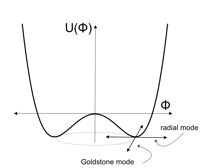
As expected, the spectrum includes a gapless Goldstone mode which is linear to lowest order in an expansion in
| (6.10) |
as well as a massive mode . To obtain this result, we have inserted the condensate from equation (6.7). As pointed out, the nature of these excitations is a key ingredient to understand superfluidity and we shall discuss their properties in detail in the chapters to come. By now, we have discussed all microscopic concepts necessary to describe superfluidity. To derive superfluid properties from field theory, it will be very important to consider modulus and phase of the condensate separately. The general setup for the upcoming calculations is described in the next chapter.
7 Lagrangian and formalism
Our starting point is the Lagrangian
| (7.1) |
with the same properties as discussed in the last section. Note however that the chemical potential is set to zero. We shall see later that it can be obtained from the (time dependency of the) phase of the Bose-Einstein condensate. For simplicity, we might also set the mass to zero in some of the results. We can now allow for Bose-Einstein condensation in the usual way by separating the condensate,
| (7.2) |
Here, is the modulus and the phase of the condensate
For convenience, we have introduced the transformed fluctuation field , which we have written in terms of its real and imaginary parts. Inserting this into the Lagrangian yields
| (7.3) |
with the tree-level potential
| (7.4) |
and the fluctuation terms, listed by their order in the fluctuation from linear to quartic,
| (7.5) | |||||
| (7.6) | |||||
| (7.7) | |||||
| (7.8) |
In the following sections, we will perform calculations in three steps:
- •
At strictly zero temperature, we can restrict ourselves to the tree level potential given by equation (7.4). In terms of the two-fluid model, this scenario corresponds to a single fluid case where only the superfluid is present. The (static) zero temperature value of the condensate is obtained from . This scenario is discussed in section 8.
- •
For low-temperature approximations, we shall need the tree-level potential and the terms quadratic in the fluctuations. The linear terms can be rewritten such that they are - up to a total derivative term - proportional to the equations of motion (8.1) and (8.2), and thus do not contribute to the on-shell action. From the contributions of , we can construct the one-particle irreducible (1PI) effective action and we will use the one-loop approximation for this quantity. While it is of course possible to construct 1PI diagrams from and , they would include external legs. The 1PI effective action includes only “legless” 1PI diagrams, the so-called “proper vertices”, as we will explain in the next section. The temperature dependent condensate can in principle be obtained from the stationary equation . However, we will approximate by its tree-level value. The low-temperature approximation to the two-fluid model is discussed in section 10.
- •
To go beyond the low-temperature limit, we will use a two-particle irreducible (2PI) formalism. In the 2PI framework, contributions from and obviously cannot be neglected. All diagrams which are two-particle irreducible and can be constructed from the interaction terms above are collected in the potential (see figure 7.1). The “double-bubble” diagram can be directly constructed from . From alone it is not possible to construct a 2PI diagram. We can see however that every vertex in contains a condensate, and as we know, each condensate comes with a factor of (see equation (6.7)). Therefore, to order we have to include second order contributions from which are given by the second diagram in figure 7.1. The one-particle and two-particle irreducible effective action will be derived in section 9. The 2PI effective action is a functional of the condensate as well as the full propagator . The stationarity equations and not only allow for a self consistent determination for the condensate but also of the mass parameter. This is important for the following reason (see also discussion in reference [50]): consider the simplest case with no condensation (and no superflow). The dispersion relations (6.9) then reduce to the simple form
Condensation occurs for in which case acquires an unphysical negative value. A non-vanishing condensate leads to corrections proportional to in the propagator, see (6.8). The resulting dispersions (6.9) are then positive for all three-momenta and can be used to calculate thermal integrals in the low-temperature approximation. However, as the condensate is expected to melt away at the critical temperature, this problem will indefinitely occur for sufficiently large temperatures if the mass remains fixed. Therefore, self-consistency equations for mass and condensate are required. Calculations for arbitrary temperatures are discussed in section 11.

8 Zero temperature: Single fluid formalism
In a first step, the translation of field theory into hydrodynamics will be carried out at tree-level, ignoring all quantum fluctuations. This allows us to present the translation into hydrodynamic equations in the simplest case, based on reference [85]. We begin with a discussion of the conservation equations as well as the equations of motion and solutions thereof.
8.1 Equations of motion and conservation equations
The classical equations of motion for and are
| (8.1) | |||||
| (8.2) |
The field-theoretic expressions for the conserved charge current and the stress-energy tensor are
| (8.3) | |||||
| (8.4) |
For the stress-energy tensor, we have used the gravitational definition by formally introducing a general metric which, after taking the derivatives, we set to be the metric of flat Minkowski space. This definition guarantees that is symmetric and conserved. Since is also conserved, we have
| (8.5) |
which are the hydrodynamic equations. As we expect from Noether’s theorem, current conservation is identical to the equation of motion for . The reason is that only appears through its derivatives in the Lagrangian, as it should be for the radial mode in the presence of an exact U(1) symmetry.
As an ansatz for the solution of the equations of motion we may choose
| (8.6) | |||||
| (8.7) |
In this ansatz, we assume and are each composed of a static part plus small oscillations around it. The static part of the solution is the superfluid mode, corresponding to an infinite and uniformly flowing superfluid. The density and flow are specified by the values of the components of , which are pure numbers, not functions of , and are not constrained by the equation of motion. The value of is determined by the boundary conditions, which specify the topology of the field configuration, namely the number of times the phase winds around as we traverse the space-time region in which the superfluid resides2626 26 Usually, Bose-Einstein condensation is introduced by separating the zero momentum mode in the expansion of This case however corresponds to the separation of the mode resulting in is given by from equation (8.8). . The oscillations around the static solution yield two modes whose dispersion relations are determined by the equations of motion. As expected, one of the modes is the massless Goldstone mode, the other is a massive “radial” mode (see also figure 6.3). The oscillatory modes can be thermally populated to yield the normal fluid. The boundary conditions place no constraint on the amplitudes of the oscillatory modes because they are topologically trivial. In this section we will assume uniform density and flow of the superfluid, but in general one could obtain a space-time-dependent superfluid flow by giving nonzero classical background values to the and . The normal fluid would then consist of a thermal population on top of that background. We can use the poles of the tree-level propagator (10.2) to determine the dispersion relation of the oscillatory modes. This yields the same result as solving the equations of motion (8.1), (8.2) with the ansatz (8.6), (8.7). Oscillations in will also be relevant to the calculation of the sound velocities. In fact, for low temperatures we will demonstrate that the coefficient of the linear term in the massless mode is nothing but the velocity of first sound. For now, we set . In this case, , and we can write
| (8.8) |
Inserting this solution back into the Lagrangian gives
| (8.9) |
It is clear from the usual definition of the pressure in terms of the partition function that, in our current tree-level treatment, this Lagrangian is identical to the pressure. Bose-Einstein condensation obviously appears for which is a first hint that plays the role of a chemical potential. It is important to keep in mind that we will keep the approximation of uniform density and flow of the superfluid throughout the remainder of this work, including the finite temperature calculations of sections 10 and 11.
8.2 Zero-temperature hydrodynamics: Landau‘s formalism
We now explore the connection between field-theoretic quantities and hydrodynamics. We recall that the hydrodynamic expressions for current and stress-energy tensor at zero temperature are:
| (8.10) | |||||
| (8.11) |
where is the velocity of the superfluid which fulfills . To identify , , and we go to the superfluid rest frame = (1,0,0,0), where there is no flow of charge, energy, or momentum: . Then we have , , , so , , and are the charge density, energy density, and pressure in the superfluid rest frame; the pressure is isotropic. (We will discuss the superfluid density below). They can be expressed covariantly via appropriate contractions,
| (8.12) |
To relate these hydrodynamical quantities to the microscopic physics we can use equations (8.3), (8.4). For and we obtain immediately
| (8.13) |
where is the superfluid 3-velocity with Lorentz factor . This is precisely the factor multiplying when measured in the normal-fluid rest frame (see table 1 in section 5.4). The velocity is given by 2727 27 The minus sign appears because the 3-velocity corresponds to the spatial components of the contravariant 4-vector , while the operator corresponds to the spatial components of the covariant 4-vector , i.e.,. We have thus recovered the expected irrotational flow of the superfluid. The difference between expressions (8.13) and (5.27) is that we have identified the scalar potential as the phase of the condensate. For and we first use (8.12) and (8.4) to obtain partly microscopic expressions
| (8.14) |
From contracting the relation for in (8.13) with we know that ; as a consequence, we obtain the expected relation . We can now identify the physical meaning of : using the zero-temperature thermodynamic relation in the superfluid rest frame , we find
| (8.15) |
so is identified with the chemical potential in the superfluid rest frame. Going back to the solution for the modulus (8.8) we see that, as expected, Bose condensation only occurs for . Using (8.9) and (8.14) we finally obtain fully microscopic expressions for the energy density and the pressure,
| (8.16) |
Note that is the only mass scale in our Lagrangian. The trace of the stress-energy tensor vanishes for . Finally, the superfluid density is defined via the expansion in small three-velocities of the momentum and energy densities
| (8.17) |
From these expansions we obtain its microscopic form
| (8.18) |
8.2.1 Generalized single fluid formalism
We can now repeat the above translation in the frame of the generalized hydrodynamic formalism. Although this might seem to be an unnecessary complication for the isotropic zero-temperature case, it is a useful preparation for the nonzero temperature case. The basic variables are the conserved current density and its conjugate momentum. We will now confirm that this conjugate momentum is given by the gradient of the phase . Recall that in the single fluid case the stress-energy tensor is given by
| (8.19) |
with the generalized pressure and the generalized energy density is given by
| (8.20) |
This is the Legendre transform in the single fluid case where , and . By comparison with the expressions from section 8.2, it is easy to see that in the single-fluid case and are simply pressure and energy density in the fluid rest frame (see also discussion in section 5), , . In the single fluid case, the current is indeed proportional to the conjugate momentum with a coefficient given by the underlying microscopic physics
| (8.21) |
and
| (8.22) |
where we can simply read off
| (8.23) |
In summary, it is important to keep in mind that the connection from macroscopic to microscopic physics is made by identifying the conjugate momentum as the four-gradient of the phase of the condensate. In addition, in equations (8.13) -(8.16) we express all thermodynamic and hydrodynamic parameters of the Landau model in terms of field theoretic variables while the microscopic physics enter the generalized hydrodynamic formalism via the coefficient from equation (8.23). In addition, from equation (8.13) and (8.15) we draw the following important conclusions:
- •
The rotation of the phase (at the bottom of the “Mexican hat” potential) generates the chemical potential of the superfluid.
- •
The number of rotations per unit length determines the superfluid velocity.
- •
represents the invariant expression for the chemical potential . In case this relation simplifies to . In case we have . Here we have indicated that alone is not an invariant and therefore changes its value to when measured from outside the superfluid rest frame. The Lorentz factor in compensates this change such that is indeed invariant.
8.2.2 The non-relativistic limit
The relativistic two-fluid equations incorporate the correct non-relativistic limit of section 2 (for a general discussion, see for example [67]). In this section we investigate this limit in the single fluid case at zero temperature. According to Landau and Lifschitz [87] we need to write the relativistic energy density as the sum of the rest energy of particles that constitute the fluid and the non-relativistic energy density . Here is the particle number per volume in the rest frame of the fluid. To transform into the laboratory frame (i.e. to eliminate in favor of ), we write the energy density as 2828 28 For notational consistency, we still omit factors of which are usually taken into account in the non-relativistic literature. :
| (8.24) |
In the single fluid case, the components of can be written as
| (8.25) |
Here, we have inserted the factor contained in definition of . Expanding for small velocities and inserting from equation (8.24), reads
| (8.26) |
Here, we have used that the non-relativistic pressure and energy density are much smaller than the rest energy: . After subtraction of the rest energy , we obtain the expected result
| (8.27) |
Next, we expand up to the third order in resulting in
| (8.28) |
where again has been used. The result reads:
| (8.29) |
In the non-relativistic case momentum density and energy flux are not the same. To obtain , we need to subtract the term coming from the rest energy first and obtain
| (8.30) |
Analogously we obtain the spatial components:
| (8.31) |
9 The 1PI and 2PI effective action
In this section, we review the one-particle irreducible (1PI) and two-particle irreducible (2PI) formalism which we shall apply in the finite temperature calculations. Both formalisms are non-perturbative in the sense that the coupling constant is present to all orders and a certain class of diagrams is resummed. We have discussed in section 7 that such a non-perturbative and self-consistent formulation is necessary to extend our calculations to finite temperatures. We can restrict the discussion in this chapter to the zero temperature case. In the imaginary time formalism, the introduction of finite temperature amounts to a “straightforward” modification of the results which we will obtain in the following. As a preparation, it is necessary to discuss the difference between full, connected and 1PI diagrams.
9.1 Full, connected and one-particle irreducible Green‘s functions.
In what follows, bare propagators are represented by , interaction vertices by and sources (sinks) by . The abstract index represents continuous as well as discrete parameters such as space-time or the internal internal space spanned by the fields and . We consider only the bosonic case where the ordering of is irrelevant. For the purpose of introducing the 1PI and 2 PI formalism, we shall denote a bosonic scalar quantum field by and a corresponding classical field by . Later, when we perform actual calculations, we will denote the classical field simply by (we have already done so in section 6.2).
Physical processes, algebraically expressed in terms of Green‘s functions, can be graphically illustrated by Feynman diagrams. The full n-point Green‘s function defined as the time-ordered vacuum expectation value of Heisenberg field operators corresponds to an infinite sum of Feynman diagrams which take into account all possible interactions as we discuss in figure 9.1. The Dyson-Schwinger equation (DSE) represents a systematic way to generate all these diagrams.

One can see right away that the DSE is self-consistent and it is exact only if all diagrams can be resummed (which is practically never the case). In principle, the DSE can be used to reproduce the perturbative expansion of a given theory to arbitrary order by iteration (see for example [89]). We define the functional from which we can generate all vacuum Green´s functions for a process with different sources. (Since depends on continuous as well as discrete parameters, it is a functional.) Obviously, we can obtain the full N point Green‘s functions by acting on with (functional) derivatives:
| (9.1) |
This allows us to express the DSE as:
| (9.2) |
Collecting bare (inverse) propagators and vertices in the definition of the action of the field
| (9.3) |
and using:
| (9.4) |
we can elegantly write the DSE for any full N-point functions as:
| (9.5) |
This equation is the quantum version of the classical equation of motion which is given by
| (9.6) |
As an example, we perform one iteration of the DSE for a full three-point function in figure 9.2. As we can see, the result is a factorization into mutually connected and disconnected diagrams which represents a new way of decomposing all Feynman diagrams.

This factorization is graphically illustrated in figure 9.3. Formally, one can write this factorization for an arbitrary N-point function as:
| (9.7) |
where , the generating functional of all connected Green‘s functions , is defined in exactly the same way as (with the index starting from 1 as there is at least once source attached to a connected Green‘s function):
| (9.8) |
The differential equation (9.7) relating and can easily be solved resulting in
| (9.9) |
Using this relation, one can easily construct the DSE in terms of connected diagrams from (9.5). Taking into account the chain rule
we find the following elegant formulation of the DSE in terms of connected Green´s functions
| (9.10) |
Finally, we can further decompose connected Green‘s functions in terms of one-particle irreducible (1PI) ones. By definition, 1PI Green‘s function remains connected even if one internal line is cut. If one follows an external leg into a connected Green‘s function one inevitably ends up on a 1PI diagram which again has zero, one or more external legs which lead to another connected part and whose cutting would disconnect the diagram (at tree level, one does not end up at a 1PI diagram at all). Iteration leads to yet another decomposition in terms of 1PI diagrams. This is summarized in figure 9.4.

The 1PI Green‘s functions can be viewed as the fundamental building blocks of any Feynman diagram. The coefficients in this expansion are called proper self energy (connecting two external legs) and proper vertices (connecting three or more external legs). We introduce the field , a connected Green‘s function with one external leg attached. This object is precisely the classical field
defined as the vacuum expectation value of the quantum field in the presence of an external source
Here, we have defined the proper self energy as . The reason for this definition is that we want to reformulate equation (9.12) such that the left side is zero:
| (9.13) |
Again we introduce the corresponding generating functional:
| (9.14) |
where the argument of denotes a vector of the classical fields . Acting with on generates vertices of 1PI diagrams - unlike full or connected Green‘s functions, 1PI Green‘s functions do not have propagators attached on their external legs. With these preparations, we can reformulate equation (9.13) in the following way
| (9.15) |
Equations (9.15) reveal the true nature of the relationship between connected and 1PI green functions: and are connected by a Legendre transform
| (9.16) |
This equation summarizes that is independent of and is independent of
| (9.17) |
Once again, we can construct the DSE in terms of 1PI diagrams. To do so, we eliminate derivatives
in favor derivatives of :
| (9.18) |
and further use and to exchange with in the DSE (9.5):
| (9.19) |
The 1PI DSE equation (9.15) still plays the
role of a quantum analog to the classical equation of motion. Motivated
by equation (9.19), is called effective
action. To obtain the classical equation of motion from the 1PI quantum
DSE (9.19), we can simply neglect the contribution coming
from . The role of is to create
loops. 2929
29
The classical DSE can be obtained from (9.19)
by neglecting the contribution coming from . It
is a tree expansion of the form
We can interpret the right hand side diagramatically:
![[Uncaptioned image]](1502.00122v1/classicExp.png) Comparing this to the 1PI expansion displayed in figure
9.4, we can see that the vertices of
the tree expansion have been replaced by 1PI diagrams. In other words
in the 1PI formalism, the quantum loop corrections to the classical
expansion are embodied in the proper vertices ,
i.e. they sit in the spot of the classical vertices.
Comparing this to the 1PI expansion displayed in figure
9.4, we can see that the vertices of
the tree expansion have been replaced by 1PI diagrams. In other words
in the 1PI formalism, the quantum loop corrections to the classical
expansion are embodied in the proper vertices ,
i.e. they sit in the spot of the classical vertices.
In summary, we can take the generating functional of full Green‘s functions, replace with and and instead of evaluating the full path integral substitute the classical approximation in the integrand and obtain an exact result.
Spontaneous symmetry breaking manifests itself in the 1PI formalism by a nonzero vacuum expectation value of , even though the source J is set to zero
| (9.20) |
9.2 1PI effective action in the one loop approximation
In order to obtain the one loop approximation for the effective action for a complex scalar field we introduce the path integral representation for the generating functional of connected Green‘s functions
| (9.21) |
Next, we perform the Legendre transform to obtain the 1PI effective action
| (9.22) |
and expand the action around the classical solution which is the main contribution to the path integral
| (9.23) |
This amounts to
| (9.24) |
Inserting the result in the exponent of (9.22) and performing the Gaussian integral3030 30 The linear shift in doesn’t affect the integration measure. yields
and therefore
| (9.25) |
where det M=exp[Tr ln M] has been used. This is the one loop effective action which we shall use (within certain approximations) in section 10.1. The term proportional to the quadratic fluctuations is the propagator, see for example (6.8). In summary, the Legendre transform has introduced new vertices to our theory. To check that the diagrammatic expansion of is indeed given by all one loop diagrams of these vertices, we separate contributions from the condensate which are resummed to all orders in in (9.25), from the free propagator in absence of a condensate , where is matrix of the dimension of the internal space3131 31 Comparing to our case of a complex scalar filed, and are given by The situation will be slightly more complicated once we treat modulus and phase of the condensate separately (see also (7.6)) as becomes anisotropic..
Then the logarithmic term is decomposed as follows
We can now expand the second term in a Taylor series and obtain
Diagrammatically, this series corresponds to a one loop diagram with 2, 4, 6.. classical fields (condensates) attached:
![[Uncaptioned image]](1502.00122v1/1PIPot.png)
As expected, no external legs are connected to these 1PI diagrams. A more physical way to say this, is that external legs would introduce a momentum dependence of . We will later identify this functional with the pressure, which, being a thermodynamic quantity, must not depend on external momenta.
9.3 Two-particle irreducible formalism
The construction of the 2PI effective action is a straightforward generalization of the 1PI case. As a starting point we use the generating functional of connected Green‘s function and introduce two source terms, one for the quantum field and one for the quantum propagator :
| (9.26) |
The classical field and two point function (propagator) are obtained in the usual way:
| (9.27) |
and therefore variation with respect to the source results in
Before we turn to the construction of the 2PI effective action, we remark that we can easily construct the 1PI effective action of the functional (9.26). The quadratic term including can formally be treated as an additional “mass” term and the (single) Legendre transform can be directly applied:
| (9.28) |
In analogy to the 1PI effective action, we define now the 2PI effective action by a double Legendre Transform with respect to and
| (9.29) |
Furthermore, the equations of motion for the fields and are given by
| (9.30) | |||||
| (9.31) |
Using equation (9.27) and the 2PI effective action (9.29), it is again easy to show that and . The physically interesting case is again given by vanishing sources in which case the equations of motions turn into
| (9.32) |
with non-vanishing expectation values and . What is remarkable about the stationary equations (9.32), is that they already include the DSE for the propagator on the classical level. We shall exploit this fact extensively in section 11. In particular cases such as BCS theory, spontaneous symmetry breaking does not result in a vacuum expectation value of the field, but in a vacuum expectation value of the two point function. The 2PI formalism is therefore particularly well suited to describe such systems. In the path-integral representation, the 2PI generating functional is given by
We can again study the loop expansion systematically. To leading order, we can use the one loop approximation derived in the last section to evaluate the 1PI effective action defined by (9.28) (i.e. we use the generating functional from equation (9.26) but perform only a single Legendre transform with respect to ). Remember that we can absorb the term proportional to as an additional mass term into the propagator of the action . Now all we have to do is to replace by and the free propagator in the background of the classical field by in the expansion (9.23). The result reads:
From the dual Legendre transform (9.29) we can obtain the one loop approximation of the 2PI functional:
To reformulate this equation in a more useful way, we need to eliminate the remaining source in favor of the field . This can be achieved with the aid of from which we obtain (at lowest loop order) and therefore
To go beyond the one loop approximation, we introduce the potential which includes 2PI diagrams with at least two loops built from the propagator :
| (9.33) |
We will use the two-loop Hartree approximation of this object as will be explained in section 11.
10 Two-fluid formalism in the low-temperature approximation
10.1 Effective action and dispersion relations.
We the aid of the non-perturbative 1PI and 2PI formalisms which we have reviewed in the last section, we can now continue our derivation of the two-fluid model at finite temperature. The nonzero-temperature calculation is complicated because we are interested in the situation of a nonzero (homogeneous) superflow; this renders the system and in particular the dispersions of the Goldstone mode anisotropic. In this part, we are mostly interested in analytical results to discuss the translation to hydrodynamics thoroughly. Since we have argued in section 7 that a calculation for arbitrary temperatures requires the more complicated 2PI formalism in which results are obtained purely numerically, we shall for the moment restrict ourselves to small temperatures. In particular this means that we shall not determine the condensate self-consistently by solving , and rather work with its zero-temperature value obtained from . Starting from the full self-consistent formalism, one can show that the temperature-dependence of the condensate includes an additional power of the coupling constant compared to the terms we are keeping. We are thus working in the low-temperature, weak-coupling approximation. Note however that the melting of the condensate, as well as other contributions from the full action may induce terms proportional to in the pressure, while we shall only keep terms proportional to and higher order in . This approximation is only consistent if , i.e., strictly speaking, our approximation leaves a “gap” between and the small temperatures we are discussing, although this gap can be made arbitrarily small by choosing the coupling constant sufficiently small.
Within this approximation, we can work with the simple 1PI effective action in the one-loop approximation
| (10.1) |
with the tree-level potential from equation (8.9) and the inverse tree-level propagator in momentum space which can be read off from the terms quadratic in the fluctuations in equation (7.6). The trace is taken over the space of the two real degrees of freedom of the complex scalar field, and the sum is taken over four-momenta , with the bosonic Matsubara frequencies . The sum over three-momenta, here written for a finite volume and thus over discrete momenta, becomes an integral in the thermodynamic limit. At the stationary point, i.e., with equation (8.8), we have
| (10.2) |
Here, , and . In all our microscopic calculations we evaluate thermal fluctuations in the background of a uniform superflow, so we take (and hence ) to be space-time independent3232 32 Observe that the relation between with and without superflow is given by a simple boost. To see this, set in (10.2) and then boost every wave vector by an arbitrary velocity : This results in Inserting the microscopic expressions and we arrive precisely at (10.2). .
Since we neglect the melting of the condensate, we have inserted the zero-temperature solution into the propagator. In order to compute the effective action, one may employ partial integration with respect to the integral. The effective action density then becomes
| (10.3) | |||||
where we have used the explicit form of the tree-level propagator and have performed the trace. We have also inserted the zero temperature solution for into the potential . The evaluation of the Matsubara sum and the simplification of the result are explained in detail in appendix A. Neglecting the thermal contribution of the massive mode, we can write the result as
| (10.4) |
where denotes the numerator in the momentum sum of equation (10.3)
| (10.5) |
and where are complicated excitation energies whose small-momentum approximations are
| (10.6) | |||||
| (10.7) |
Here we have abbreviated
| (10.8) |
with being the angle between and . The physically relevant low-energy excitation is . This is the Goldstone mode which, as equation (10.6) confirms, is massless and linear in the momentum for small momenta, as it should be. The coefficient in front of the linear term is related to the speed of (first) sound as we explain in part III. For the case without superflow we have , and thus, in the limit , we recover the well-known value of . The superflow introduces an angular dependence into the Goldstone dispersion and thus also into the sound velocity. This angular-dependent function also shows that, in contrast to the zero-temperature case, we cannot write the result in a covariant way since the temporal and spatial components of appear separately. Another observation is the complicated factor in the integrand of equation (10.4). This factor indicates a mixing between the original modes of the complex field (between particles and antiparticles, essentially) due to condensation. Such a factor appears also, although considerably simpler, for the case without superflow. It is analogous to a Bogoliubov coefficient in the case of Cooper pairing which, in that case, accounts for the mixing between fermions and fermion-holes. We shall now calculate the field theoretic representation of the stress-energy tensor and the Noether current.
10.2 Stress-energy tensor and current
As we have emphasized, stress-energy tensor and charge-current are particularly important in our derivation of the two-fluid model as we posses a precise recipe how to construct them from field theory:
| (10.9) |
The angular brackets denote the expectation value of an operator in the finite-temperature ensemble of the microscopic theory,
| (10.10) |
with the partition function defined so that . The calculation of the functional integral is lengthy and carried out in appendix B. The results reads
| (10.11) | |||||
| (10.12) |
In the case of the stress-energy tensor, one can check explicitly that the sum over the Matsubara frequencies leads to an infinite result. A renormalization is thus required. As a renormalization condition, we require for the case without superflow the obvious interpretation of the diagonal components in terms of the energy density and the pressure ,
| (10.13) |
Then, switching on a nonzero superflow, does not yield any additional divergences. These conditions can be implemented on a very general level, without explicit evaluation of the stress-energy tensor. We do so in detail in appendix C. The calculation in this appendix also leads to a very useful formulation of the effective action, the stress-energy tensor, and the current, which will later facilitate the interpretation in terms of the hydrodynamic two-fluid picture. We define
| (10.14) |
and
| (10.15) |
In the zero-temperature discussion, we have related the tree-level potential to the generalized pressure . The notation of equation (10.14) anticipates that we can identify the effective action with the generalized pressure at finite temperature. In section 10.3, we will see that this assumption is justified. The notations , , are chosen in analogy to , , , which we introduced in section 5.1 (we already know the zero temperature contribution to the coefficient from the single-fluid treatment of section 8.2.1). With the help of these quantities we can rewrite the effective action as (see appendix C)
| (10.16) |
where we have abbreviated , while the renormalized stress-energy tensor and the current become
| (10.18) |
These expressions are useful because, firstly, they are written in a covariant way and, secondly, they anticipate the two-fluid formulation which as we know is constructed from two basic four-vectors. We have already identified the conjugate momentum to with ; the other conjugate momentum can of course not be identified with , which is a purely microscopic quantity, but we shall see that this formulation is close enough to the two-fluid formulation that it can easily be cast in a more “macroscopic” form. At the moment, the introduction of the four-vector is for notational purposes only, introduced to write the above equations in terms of four-vectors. We will see however that it really corresponds to the four-velocity of the normal fluid introduced in section 5.2.
It is instructive to compute the trace of the stress-energy tensor. With the help of equation (C.3) we immediately find
| (10.19) |
i.e., the trace vanishes when we set , as expected.
10.3 The two-fluid formalism from field theory
So far we have related the zero-temperature limit of the microscopic theory to hydrodynamics where we identified as the conjugate momentum to . Furthermore, we have carefully prepared field theoretic results at finite temperature, in particular the conserved current and the stress energy tensor . With these results we can continue to apply the machinery of the two-fluid formalism to successively identify all remaining hydrodynamic and thermodynamic quantities in terms of field theoretic variables. Our covariant formulation from section 10.2 before performing the Matsubara sum will turn out to be very useful for this purpose.
Before we can proceed with this program, we have to clarify the issue of frame dependence of the microscopic calculations at finite temperature once and for all. Motivated by the discussion of section 5.3, it seems reasonable to assume that the microscopic calculation is performed in the normal-fluid rest frame (or the rest frame of the heat bath) defined by . We shall now explicitly demonstrate that this is indeed consistent with the results we obtained in the last section and identify the thermodynamic parameters , and in this frame. As a first step, we may use Landau‘s definition of the charge current from equation (5.25)
and evaluate it the normal-fluid rest frame defined by . From the temporal components of we know that in the normal-fluid rest frame the total number density is given by where plays the role of a Lorentz factor (see also the discussion of table 1). While is the invariant expression of the chemical potential, clearly plays the role of the chemical potential in the normal-fluid rest frame. The superfluid velocity measured in the normal-fluid rest frame is given by . We could have introduced the normal-fluid rest frame already in the discussion of the zero temperature results in section 8.2. To avoid confusion, we have simply distinguished between results obtained in the superfluid rest frame () and outside the superfluid rest frame (). From the finite temperature point of view, measurements from outside the superfluid rest frame correspond to measurements in the normal-fluid rest frame. In case of , both fluids share a common rest frame and we have . We shall from now on denote the chemical potential in the normal-fluid rest frame by rather than (we have used the latter notation in (5.36) for the purpose of introducing both rest frames).
As a side remark, observe that we can also evaluate the spatial components of in the normal-fluid rest frame, contract the equation with and solve for . This yields
| (10.20) |
The right-hand side is now purely defined in terms of the field-theoretic quantities (the spatial components of the Noether current and the gradients of the phase ). We will however use a more systematic way to obtain the fluid densities from , and in section 10.4.1.
10.3.1 Generalized thermodynamics from field theory
Now that we have obtained chemical potential and the velocity of the superflow in the normal-fluid rest frame, we continue with the discussion of the generalized pressure and the generalized thermodynamic relation which in addition to involves the conjugate momentum . With the stress-energy tensor (5.18) and using we can write
| (10.21) |
Let us now compute the right-hand side with the microscopic expression for . With and from equations (8.4), (8.3) we compute
| (10.22) |
Here we have used , while equation (10.21) is a general relation for arbitrary four-velocities . The tensor appearing in equation (10.21) can be interpreted as a projector onto the 4-dimensional hypersurface orthogonal to . It is important to keep in mind that we cannot simply promote to an arbitrary four-velocity in the microscopic calculation. It would occur additionally in different places in the calculation, which we cannot identify in our present treatment because the spatial components of have been projected out in our finite temperature calculation. In a manner of speaking, we are “stuck” in the normal-fluid rest frame. But, of course, since is a Lorentz scalar, the normal-fluid rest frame is as good as any other frame to compute . By comparing with equation (10.16) we see that the right-hand side of equation (10.22) is exactly ( times) the effective action. Therefore, we have obtained the important result,
| (10.23) |
This relation is somewhat expected since we already know that, at zero temperature (and at tree-level), corresponds to the Lagrangian, which in this case gives the microscopic pressure. At nonzero temperature (without superflow), the effective action gives the (isotropic) pressure. Therefore, the relation (10.23) is a natural generalization to the anisotropic case with a nonzero superflow. This motivates our choice of notation in equation (10.14) because now we have
| (10.24) |
Next, let us discuss the generalized thermodynamic relation . In the normal-fluid rest frame, and thus , which is the product of entropy and temperature, measured in this particular frame. To confirm this microscopically, we use the thermodynamical definition of the entropy density,
| (10.25) |
with and defined in equation (10.15). Note that the first two terms ( and 2) come from the explicit -dependence in the prefactor and in the within the logarithm. On the other hand, we can compute via the generalized thermodynamic relation. We find
| (10.26) | |||||
where we have used , the trace of the stress-energy tensor (10.19), the effective action (which is ) (10.16), and the current (10.18). With the help of the identity (C.3) we see that this is indeed the same as times the entropy from equation (10.25). In other words, the microscopic temperature can be identified with generalized quantity in the normal-fluid rest frame. In this frame, we have now identified all terms in the generalized thermodynamic relation. By now, we have obtained the means to correctly interpret microscopic results in the frame of the two-fluid model. We shall analyze the parameters of this model now in a low-temperature approximation.
10.4 Explicit results in the low-temperature approximation
We want to compute the effective action, the components of the stress-energy tensor, and the current for small temperatures explicitly. To this end, we have to approximate momentum sums of the form
| (10.27) |
where, for the case of the effective action, is given by equation (10.5), and for the stress-energy tensor and the current we need to replace by
| (10.28) | |||||
| (10.29) |
which can be read off from equations (), (10.18). For all three cases, we can write the result of the Matsubara sum in the form (10.4). Then, we write with the Bose distribution function . The integral over the first term is, in the present approximation, temperature independent. It is divergent and has to be renormalized by subtracting the vacuum contribution. After doing so, a finite term remains which however is suppressed by one power of compared to the zero-temperature term we have already computed, for instance in equation (10.4). We shall thus neglect this contribution and only keep the thermal contribution, i.e., the integral over the second term that contains the Bose function. This contribution is finite and unaffected by the renormalization.3333 33 The subleading zero-temperature contribution we are neglecting here gives rise to the difference between the superfluid density and the condensate density. At zero temperature, the charge density is always identical to the superfluid density, , while the condensate density, defined as with the modulus of the condensate , might be smaller. In our leading-order approximation, condensate and superfluid densities are identical.We explain the small-temperature expansion in detail in appendix D. Before we come to the main results, let us discuss the simpler example without superflow, and use . In the absence of a superflow, the dispersions reduce to , with
| (10.30) |
which is equivalent to (6.9) after the condensate from equation (6.7) has been inserted. As usual, is the Goldstone mode and the massive mode. This yields the small-temperature result for the pressure to order (see also appendix F.3 for the calculation with finite mass parameter )
| (10.31) |
The term has two interesting properties related to the resulting charge density, which is obtained by taking the derivative with respect to . Firstly, if we set , the -dependence drops out, such that there is no contribution to the charge density in this case. Secondly, in the presence of a finite , one finds that the contribution to the charge density is negative, i.e., for small temperatures the density decreases with temperature. (The second derivative is positive, i.e., the system is thermodynamically stable.) The term has neither of these properties, it contributes to the charge density even for and gives rise to a positive term in the density.
The case with superflow is of course more complicated. In particular, the momentum integration now involves a nontrivial angular integral over the angle between the momentum and . Nevertheless, it turns out that this angular integral can be performed analytically for all cases we consider. For brevity, we set in the following. Then, we obtain for the effective action density to order
| (10.32) |
Obviously, for we recover the limit of equation (10.31). Note that the result is valid to all orders in the superfluid velocity. We have not applied any expansion in . Analogously, we compute the components of the stress-energy tensor and the current. For the spatial components of the stress-energy tensor we use
| (10.33) | |||||
| (10.34) |
The results are collected in table 2. All expressions in this table are written in terms of quantities measured in the normal-fluid rest frame. At zero temperature it is very natural to write them in terms of the Lorentz scalar , for instance . As expected, such a formulation is less obvious for the nonzero temperature terms. Since the microscopic calculation has a preferred rest frame where the thermodynamic variables , , and are measured, the velocity-dependence shown here is a mixture of trivial Lorentz boosts and complicated effects of the superflow on the collective excitations (which in turn can be interpreted as boosts of the microscopic vector , see footnote below equation (10.2) ).
We may compare the results presented in table 2 with the frame dependent quantities listed in table 1. One can for instance check from the explicit results that the difference between longitudinal and transverse pressure is indeed , and that the momentum density is indeed times the current . More importantly, we see that , which, since , confirms that the generalized pressure can be identified with the effective action .
With the results of in hand, we may also ask for the superfluid density . This energy density is defined in the low-velocity limit, in generalization of the mass densities in the non-relativistic framework (and in contrast to , which we calculate in the next section and which are number densities). With , , and , we obtain
(Alternatively, we can write .) This expression for the superfluid density is obviously in agreement with the zero-temperature result (8.18). The superfluid density appears also in the energy density as part of the kinetic energy, .
10.4.1 Entrainment and superfluid density from field theory
The independent degrees of freedom of our microscopic calculation are the chemical potential , the temperature , and the superfluid three-velocity , all measured in the normal-fluid rest frame, where the entropy current vanishes by definition, . We have thus given 8 independent components out of the 16 components of the 4 four-vectors , , , of the two-fluid formalism. The other 8 components are , , and . For the Noether current and the entropy we have field-theoretic and thermodynamic definitions respectively. It remains to compute the spatial components of the thermal four-vector . Additionally, we have to compute the coefficients , , . They are defined as the derivatives of with respect to the Lorentz scalars ,, and . However, this is not the form in which our is given. Therefore, we need to find a different way to compute these coefficients. This can be done with the help of equations (5.8) and (5.9). First, we solve the spatial part of equation (5.8) for and insert the result into the spatial part of equation (5.9). Together with the temporal components, this yields three equations for the three variables , , , whose solutions are listed in table 3, where, for completeness, we also give the coefficients , , , which are obtained from the inverse of equation (5.11). With these results we immediately find
| (10.35) |
Since all results are expressed in terms of quantities accessible from our microscopic calculation, we can for instance compute (for and in the low-temperature limit)
| (10.36) | |||||
| (10.37) | |||||
| (10.38) |
We see that the coefficients and vanish at . This is in accordance to our zero-temperature discussion, where only was nonzero. The connection between the coefficients , and the number densities , is given in equation (5.31). We can insert and as functions of , into the temporal component of equation (5.6) to get also as a function of , . The result is the useful translation
| (10.39) |
(To avoid confusion: , , , are quantities measured in the normal frame, while is the superfluid density measured in the superfluid frame. Remember that the superfluid density measured in the normal frame is .) As a check, we see that given in table 3 is indeed the same as with calculated from equation (10.20). It is now of course straightforward to also express , , in terms of and . In the small-temperature approximation, the superfluid and normal number densities, measured in the normal-fluid rest frame, become
| (10.41) |
One can check that the sum of both densities gives the total charge density from table 2. As expected, the normal density vanishes for and begins to increase with increasing temperature, while the superfluid density decreases. In the more complete treatment of section 11, we expect the superfluid density to vanish at the critical temperature because the condensate melts. Remember that this melting is, in our one-loop effective action, a higher-order effect in the coupling constant, which we have neglected. The decrease of is therefore only due to the interaction between the two fluids. As an aside, note that for the contributions in superfluid and normal densities cancel each other exactly. We have made this observation already below equation (10.31) where we have seen that in the limit there is no contribution to the density.
Finally, we may express the generalized pressure in terms of Lorentz scalars. This reformulation is instructive because it gives in the form that is usually assumed in the two-fluid formalism.
Our quantities in the normal-fluid rest frame , , are translated into the relevant Lorentz scalars , , via
| (10.42) | |||||
| (10.43) | |||||
| (10.44) |
We solve these equations for , , and and insert the result into the effective action. Then, up to fourth order in the temperature we can write the generalized pressure as
| (10.45) |
The term in the square brackets can be written as with the “sonic metric” , see equation (8.9) of reference [83]. In other words, the Lorentz invariant term of the pressure in the presence of a superflow is obtained by replacing in the term of the pressure in the absence of a superflow. In principle, we can use the higher order terms in equation (10.42-10.44) to write the contribution in terms of Lorentz scalars. However, we have not found a compact way of writing this contribution. But, we have checked that it is not simply given by the same replacement as for the term. This is no surprise since the sonic metric is constructed solely for systems for a Goldstone mode with linear dispersion. The term however, knows about the cubic term in the dispersion.
10.5 Conclusion
We have discussed the dissipationless hydrodynamics of a relativistic superfluid, starting from a complex scalar field. Our main goal has been to relate the field theory with the covariant two-fluid framework of superfluidity. To achieve these goals analytically, we have so far restricted our calculations to the limit of small temperatures. The results from these studies and the approximations necessary to obtain them shall now be summarized.
- 1.
Microscopic calculation. We have started from Bose-Einstein condensation in a theory. The condensate has been assumed to be static and homogeneous (which corresponds to the simple hydrodynamic scenario of a static, homogeneous superflow). A crucial role is played by the phase of the condensate. While small oscillations of the phase correspond to the excitations of the Goldstone mode, rotations of the phase around the full circle give rise to a chemical potential (speed of the rotation) and a superfluid three-velocity (number of rotations per unit length). In the presence of a non-zero superflow, the excitations of the Goldstone mode become anisotropic, and we have computed the resulting components of the conserved current and stress-energy tensor for nonzero temperatures. We have restricted ourselves to a weak-coupling, low-temperature approximation, including terms up to sixth order in the temperature. This has allowed us to present the microscopic results in an analytical form.
- 2.
The two-fluid formalism. In the relativistic two-fluid formalism, the basic variables are the charge current and the entropy current. In the dissipationless case, both are conserved. For both currents, we can define conjugate momenta. Now, if the two fluids are interacting with each other, neither of the currents is (four-)parallel to its own momentum, but also receives a contribution from the other momentum. This contribution is called entrainment, and it must be computed from an underlying microscopic theory. This formalism was explained in detail in sections 5 and 5.2 where different formulations based on “mixed” and “pure” variable sets where described and related to each other. For instance, the entrainment coefficient (and related coefficients) can be expressed in terms of the superfluid and normal-fluid charge densities and (whose corresponding superfluid and normal-fluid four-currents are, even in the dissipationless case, not separately conserved).
- 3.
Relationship between them. There are several concepts and quantities in the two-fluid formalism that are usually not used in field theory, such as the generalized pressure that depends on Lorentz scalars. Therefore, one important aspect of this work has been a translation of these quantities into field-theoretic language. For instance, we have proven that, once we assume that the microscopic calculation is performed in the rest frame of the normal fluid, it follows that the generalized pressure is given by the effective action. We have also expressed the coefficients that relate the currents with the conjugate momenta in terms of quantities that are well defined in field theory, namely the space-time derivative of the phase of the condensate, the components of the Noether current, and the entropy. As a result, we have been able to compute these coefficients explicitly as a function of temperature, chemical potential, and superfluid velocity. Certain combinations of these coefficients yield and . Our calculation shows for instance that is not simply given by the condensate density: even though we have neglected the temperature dependence of the condensate, depends on temperature. It also confirms that is not identical to the phonon number, as one might naively expect; while the phonon number goes like for small temperatures (see for instance [90]), .
11 The two fluid model at arbitrary temperatures
We will now go beyond the low-temperature approximation (i.e. extend calculations up to the critical temperature), and go beyond the weak-coupling limit by resumming certain contributions to all orders in the coupling constant. We still neglect dissipation and keep the superflow uniform in time and space. In the extension to high temperatures we have to make use of the more elaborate 2-particle irreducible (2PI) formalism [91, 92, 93] (also called Cornwall-Jackiw-Tomboulis (CJT) formalism or -derivable approximation scheme) which we have introduced in section 9.3. We will use this formalism in the Hartree approximation at two-loop level. We have seen that this formalism is particularly well suited to systems with spontaneously broken symmetries. It has been used previously, among many other applications, to describe meson condensation in the CFL phase [94, 50, 95], but without including the effects of a superflow. This is the first time that a superflow has been implemented in this formalism. The extension to all temperatures below the critical temperature for superfluidity is relevant in the context of compact stars because temperatures in the star may well be of the order of the critical temperature or higher, in particular in its early evolutionary stages.
11.1 The effective action in CJT
Based on the results of section 10.3.1, we relate the 2PI effective action which is a functional of the (modulus of the) condensate and the full propagator , to the generalized pressure . Remember that the index “c” for classical fields and propagators will be suppressed. In the two loop approximation, the effective action density ( times the effective action) is then given by (see equation (9.33))
| (11.1) |
where the trace is taken over the internal space and is the three-volume. The the potential includes all two-loop, two-particle-irreducible, diagrams. These diagrams are shown in figure 7.1. Here, we have used the definitions of the tree level potential
| (11.2) |
and the free propagator in the presence of a condensate
| (11.3) |
For convenience, we first discuss the unrenormalized effective action and include a counterterm later, see section 11.2 and appendix E. The Hartree approximation implies that we only consider self interaction terms coming from the “double bubble diagram” (left diagram in figure 7.1). The exchange contributions to coming from the “sunset diagram” (right diagram in figure 7.1) are neglected. We are thus left with a single two-loop diagram which is generated by the quartic interactions and whose algebraic expression is
| (11.4) |
Had we included the “sunset diagram” originating from the cubic interactions, would also depend explicitly on . Moreover, the self-energy would depend on momentum. Therefore, neglecting the contribution from the cubic interaction is a tremendous simplification, even though only an explicit calculation can show whether its contribution is indeed small. Naively, the additional factor of the condensate at the cubic vertex suggests that for chemical potentials only slightly above the mass our simplification is a good approximation. However, it was that shown the contribution we neglect is important to obtain a second order phase transition, i.e., the Hartree approximation shows, unphysically, a first order phase transition [96, 97, 98]. We shall come back to this issue when we present our results in section 11.4.
In our approximation the self-energy does not depend on momentum and is given by
| (11.5) |
where the first term is proportional to the unit matrix. One can now easily confirm the useful relation
| (11.6) |
To determine the ground state of the system, we need to find the stationary points of the effective action. To this end, we take the (functional) derivatives of the effective action with respect to and
and set these to zero,
| (11.7) | |||||
| (11.8) |
With an ansatz for the full propagator we can bring these equations into a more explicit form. Within the present approximation, the most general form of the propagator is [50]
| (11.9) |
with two mass parameters , , that have to be determined self-consistently. With this ansatz, the off-diagonal components of the Dyson-Schwinger equation (11.8) are automatically fulfilled. We are left with the scalar equation (11.7) and the two diagonal components of equation (11.8). Inserting the first of the diagonal components into equation (11.7), and adding and subtracting the two diagonal components to/from each other, yields the following (yet unrenormalized) three equations for the three variables , , and ,
| (11.10) | |||||
| (11.11) | |||||
| (11.12) |
where and are the diagonal elements of the full propagator , and where we have already assumed that the condensate is nonzero (there is also the trivial solution which we briefly discuss in the context of renormalization, see appendix E). With the help of equation (11.6) and (11.8), the pressure at the stationary point can be written as
| (11.13) |
11.2 Renormalized stationarity equations and pressure
Renormalization in the 2PI formalism has been discussed in numerous works in the literature, for instance in references [94, 95, 98, 99, 100, 101, 102, 103, 104, 105, 106, 107, 108, 109, 110]. For our purposes, the methods developed and used in references [94, 95, 103] are most useful. While reference [103] introduces counterterms “directly” in the effective action, [94, 95] use an iterative method, based on [101, 102], where the counterterms are introduced order by order in the coupling. Both methods are equivalent. We shall follow the “direct” approach of [103]. All details of the renormalization are discussed in appendix E. Here we simply summarize the main steps and give the results.
The renormalization requires to add appropriate counterterms to the effective action (11.1), proportional to the (infinite) parameters , , . In the condensed phase, two different parameters , for the renormalization of the coupling are necessary. Then one can show, after regularizing the ultraviolet divergent integrals in the action and the stationarity equations that the parameters , , can be expressed in terms of the (finite) renormalized parameters , , an ultraviolet cutoff , and a renormalization scale . And, importantly, these parameters do not depend on the medium, i.e., on , , and . The relation between the cutoff dependent quantities and the renormalized ones becomes a bit more compact if we introduce (infinite) bare parameters via , . Then, we can write the renormalized parameters as
| (11.14) |
For the regularization of the divergent momentum integrals we use Schwinger’s proper time regularization [111], where the cutoff is introduced by setting the lower boundary of the proper time integral to . More precisely, we separate a “vacuum” contribution from each of the divergent integrals such that a finite integral remains and the “vacuum” term can be regularized. This term is not exactly a vacuum term because the ultraviolet divergences depend on the self-consistent mass (and thus implicitly on , , and ), and therefore the subtraction term must be (implicitly) medium dependent. In the presence of a superflow, we even find that the ultraviolet divergences depend explicitly on , see discussion in section E.4.
To write down the result of the renormalization procedure we first introduce the following abbreviations for the momentum sums,
| (11.16) | |||||
| (11.17) | |||||
| (11.18) |
where the finite parts of the momentum sums are
| (11.19) | |||||
| (11.20) | |||||
with the Euler-Mascheroni constant , the Bose distribution function , and the quasiparticle excitations that are given by the positive solutions of . The energies
appear in the “vacuum” subtractions whose regularized versions give rise to the (medium dependent) finite terms in the first lines of equation (11.19) and (11.20) and to (medium independent) infinite terms which are absorbed in the renormalized coupling constant and the renormalized mass.
The renormalized version of the pressure at the stationary point is
| (11.21) |
with , , and being solutions of the stationarity conditions (11.16-11.18), and the finite part of
the momentum sum
| (11.22) | |||||
11.3 Goldstone mode
The quasiparticle dispersion relations are determined by the zeros of . In analogy to the zeros of which lead to the dispersions (10.6), (10.7) we expect one massive mode and one Goldstone mode where the Goldstone mode fulfills at . Setting in the inverse propagator (11.9), we see that is only a zero of if (or if ). However, this condition for the existence of a Goldstone mode is in contradiction to equations (11.16) and (11.18) which imply , where might be small but does not vanish. Consequently, the Goldstone theorem is violated in our approach [50, 94, 95, 99, 100, 103, 104, 106, 108, 109, 110]. For our discussion of the superfluid properties it is crucial to work with an exact Goldstone mode. Therefore, we shall ignore the contribution from the momentum sum in equation (11.18), thereby giving up the exact self-consistency of our approach [50, 104]. This is an ad hoc modification of the stationarity equations, i.e., we do not consider the true minimum of the full self-consistency equations, but a point away from this minimum. The benefit of this modification is that the Goldstone theorem is built into our calculation. Of course, our choice of enforcing the Goldstone theorem is not unique, and there are infinitely many “Goldstone points” once the exact self-consistency is sacrificed. This situation is illustrated in figure 11.1. A similar, but not identical, procedure is followed in reference [108], where the stationary point in the constrained subspace given by the condition of an exact Goldstone mode is determined.

Our modification results in a particularly simple set of equations, because the three stationarity equations now reduce to two trivial ones and only one that still contains a momentum integral,
| (11.23) | |||||
| (11.24) |
The two dispersion relations are then determined from
| (11.25) |
where equation (11.23) has been used to eliminate . Since we are interested in arbitrary temperatures below , we shall need the full dispersion of both modes. Their explicit form is too lengthy to write down, but we can at least demonstrate the linear part of the dispersion relation of the Goldstone mode as a function of the mass parameter (this result is identical to (10.6) if the zero temperature expression for is inserted)
| (11.26) |
For vanishing superflow we have and obtain
| (11.27) |
If we work at a point that is not exactly the stationary point, we cannot use the pressure (11.21). We rather have to evaluate the effective action density at the ”Goldstone point”. For the renormalization it is crucial that we only modify the finite part of the stationarity equations. Therefore, all infinities cancel in the same way as above, see appendix E.3 for a more detailed discussion; for the pressure at the ‘”Goldstone point” we then find
| (11.28) |
Here we have already eliminated and with the help of equation (11.24). The stationarity equation (11.24) and the pressure (11.28) are the starting point for our calculations. We shall solve the stationarity equation numerically for the self-consistent mass , which in turn gives the condensate via as well as the dispersion relations of the Goldstone mode and the massive mode. We need the pressure for various thermodynamic derivatives which are needed to compute for example the sound velocities.
11.4 Critical temperature, condensate and critical velocity for all temperatures
To get started, we need to determine the critical temperature by solving the stationarity equation (11.24) for at the point - we shall explain that this is precisely the critical value of , see discussion around equation (11.32). To do so, one has to choose specific values for the parameters and as well as , , and the renormalization scale . Then we can obtain at any temperature between and by a numerical evaluation of the stationary equation (11.24). Once we have determined from the stationarity equation we obtain the condensate through . In figure 11.2 we show the condensate as a function of temperature for the simple case without superflow and for two different coupling strengths. We have set , but the conclusions we draw from this figure are valid for all values of . As mentioned below equation (11.4), the phase transition to the non-superfluid phase turns out to be of first order, although this is barely visible if we plot the condensate for all temperatures. Moreover, there is a dependence on the renormalization scale through the logarithmic terms discussed in section 11.2. This dependence and the first order transition are very weak because of the smallness of the coupling constants chosen here. As the figure shows, the stronger the coupling, the stronger the dependence on the renormalization scale and the stronger the first order transition.
Since we know that the first-order nature of the phase transition is an artifact of the Hartree approximation, we shall restrict ourselves to sufficiently weak coupling constants. We shall work with the two couplings chosen in figure 11.2. In this case we find that we can, to a very good approximation, work with a simplified stationarity equation and a simplified pressure, using3434 34 In the notation of appendix E, this means that we approximate and .
| (11.29) | |||||
| (11.30) |
and
| (11.31) |
In this approximation, the contributions from loop diagrams that do not depend on temperature explicitly are neglected. As a consequence, the zero-temperature results are identical to the tree-level results. All dependence on the renormalization scale is gone and thus we do not have to specify . We have checked numerically that the subleading terms that we have dropped do not visibly change any of the curves we show, see also right panel of figure 11.2, where the approximation is compared to the full result.
The effects of a nonzero superflow on the solution are shown in figure 11.3, for the parameters and . In the left panel of this figure we show the Goldstone mode dispersion relation , evaluated using the value of that solves the stationarity equation. We see that for a given superfluid velocity, there is a temperature at which the dispersion becomes flat in the direction opposite to the superflow. For higher temperatures, there would be negative energies, indicating an instability of the system. Therefore, this particular temperature is a critical temperature, even though the condensate has not yet melted completely. Only at vanishing superflow is the critical temperature the same as the point where the condensate has become zero (if our approach gave an exact second-order phase transition). The plot shows that the low-energy part of the dispersion, where is linear in , is sufficient to locate the instability. Therefore, in the right panel of the figure, we show the slope of the linear part, see equation (11.26), as a function of temperature for three different values of the superflow. The superfluid state breaks down when the slope in the anti-parallel direction vanishes. This defines a critical temperature for any given velocity, or a critical velocity for any given temperature. With the help of the low-energy dispersion (11.26) we can derive a semi-analytical result for the critical velocity. We find that the linear part of the dispersion is positive for all angles between the momentum and the superflow only if . This shows explicitly that the condensate cannot become arbitrarily small for nonzero superflow. Using and , we can rewrite the condition for the positivity of the excitation energy in the equivalent, but more instructive, form
| (11.32) |
This is an implicit condition for allowed values of the superfluid velocity . (Remember that is a complicated function of this velocity.) We plot the critical line, given implicitly by equation (11.32), in the plane of superfluid velocity and temperature in figure 11.4.
The right-hand side of the inequality (11.32), evaluated at , is simply the slope of the Goldstone mode at , see equation (11.27). This is related to Landau’s original argument for the critical velocity (see also section 6.1): based on a Lorentz transformation of the excitation energy (in the original non-relativistic context a Galilei transformation), the critical velocity is determined by the slope of the Goldstone mode at (unless there are non-trivial features such as rotons in superfluid helium, which is not the case here). One might thus think that we would just have to do the calculation to determine the critical line in the phase diagram. However, switching on a superflow is not equivalent to a Lorentz transformation of the excitation energy; it is a Lorentz transformation plus a change in the self-consistently determined condensate, which in turn back-reacts on the excitation energies. This additional effect is contained in the dependence of in equation (11.32). For comparison, we have plotted the (incorrect) critical curve obtained from the dispersion in the phase diagram as a dashed line. We see that the full result is smaller for nonzero temperatures. In the weak-coupling case considered here, the effect of the superflow (in addition to being a Lorentz boost) on the Goldstone dispersion becomes negligibly small for low temperatures. Therefore, at the critical velocity is , in exact agreement with the slope of the low-energy dispersion at . For a similar recent discussion in a holographic approach see reference [112] and in particular the phase diagram in figure 6 of this reference.
The critical line seems to suggest a (strong) first-order phase transition to the non-superfluid phase at the critical velocity. However, at temperatures below ( being the critical temperature in the absence of a superflow), the system still “wants” to condense, even for velocities beyond the critical value. In other words, the uncondensed phase also turns out to be unstable. In our calculation, this is seen as follows. First we note that the stationarity equation for in the case , see equation (E.14), does not depend on . This is clear since is the phase of the condensate, so the uncondensed phase must be independent of . For supercritical temperatures the solution to the stationarity equation gives a value of that is greater than , but at subcritical temperatures is less than . The excitation energies are simply given by , so becomes negative for certain momenta if . Therefore, the non-superfluid phase is unstable below . As a consequence, within our non-dissipative, uniform ansatz, we cannot construct a stable phase for sufficiently large superfluid velocities and low temperatures (shaded area in figure 11.4). Beyond the critical velocity there may be no stable phase, if dissipative effects such as vortex creation arise in that regime. There is some evidence for this in liquid helium [113],[114] and ultra-cold bosonic [115] and fermionic [116] gases. Possibly, a more complicated, dissipative and/or inhomogeneous phase already replaces the homogeneous superfluid for superfluid velocities below our critical line. In this sense we have only determined an upper limit for the critical velocity as a function of temperature below which the homogeneous superfluid is stable. This limit can for instance be reduced by the onset of unstable sound modes due to the two-stream instability [117].
11.5 Two-fluid properties for all temperatures
11.5.1 Algorithm
Besides solving the stationarity equation we need to compute derivatives of the pressure with respect to , , and to obtain the thermodynamic and hydrodynamic parameters of the two-fluid model. As we will later also be interested in sound excitations, we need to compute all first and second derivatives. In this section, we explain the algorithm with which these results are obtained. The most direct way to do so is via brute force numerical evaluation, for instance with the method of finite differences. In order to obtain results less prone to numerical uncertainties, we compute the derivatives in the following semi-analytical way. First we note that the pressure at the point that respects the Goldstone theorem (as well as at the point where the stationarity equations are exactly fulfilled) depends explicitly as well as implicitly via on the relevant variables,
| (11.33) |
and each thermodynamic derivative we are interested in also sees the implicit dependence in . (Had we only been interested in first derivatives and had we considered the exact solution of the stationarity equations - sacrificing the Goldstone theorem - we could have restricted ourselves to the explicit dependence, since then the derivative of the pressure with respect to the self-consistently determined mass would have vanished by construction at the stationary point.) Denoting the variables by , we can thus write
| (11.34) | |||||
| (11.35) |
The derivatives of can be obtained from taking the first and second derivatives of the stationarity equation (11.24). Writing this equation as , we find
| (11.36) | |||||
| (11.37) |
We can thus use the following algorithm to compute the properties of the superfluid:
- •
Choose values for the thermodynamic parameters and as well as the parameters , , and the renormalization scale .
- •
Determine the critical temperature by solving the stationarity equation (11.24) for at the point .
- •
Find the solution for of the stationarity equation (11.24) for various values of the temperature .
- •
Compute the first and second derivatives of the integrands of and with respect to , , , and ; for the case without superflow one may use a simplification for this step as we explain below. This is done algebraically, i.e, before choosing numerical values. Nevertheless, it is useful to do all this with a computer because the results get very complicated.
- •
Perform the three-momentum integrals numerically over all expressions obtained in the previous step. Since there are three integrands (, , ) and four variables (, , , ), we have to perform integrals for the first derivatives and integrals for the second derivatives at each temperature. In the presence of a superflow, each of the integrals contains a non-trivial integration over the polar angle; without superflow, only the integrals needed for the superfluid density contain such an angular integral.
- •
Use equations (11.34-11.37), the results of the previous step, and some trivial derivatives of terms outside the momentum integrals to put together the first and second derivatives of with respect to , , and . There are many terms to handle but this is a trivial task for a computer since the non-trivial numerical calculation has already been done in the step before. We have checked that the derivatives thus obtained are much cleaner in terms of numerical errors compared to a brute force numerical calculation using finite differences.
- •
Insert the obtained derivatives into the definitions of the physical quantities such as ,, , , .
11.5.2 Limit of vanishing superflow
Even though we are also interested in the general case of a non-vanishing superflow, let us briefly discuss how the calculation simplifies in the limit . In that case, when we compute derivatives with respect to and we can set straightforwardly. But, when we compute and we have to be more careful. Consider the microscopic definition of according to (10.20). These quantities describe the response of the system to a superflow, i.e., even if we are eventually interested in the case , we need to work initially with a nonzero superflow. We can write the superfluid density for as
| (11.38) |
where we have expanded in a Taylor series for small . In this series we have dropped the linear term because the first derivative (i.e., the current ) vanishes for , which is obvious physically and can also be checked explicitly. It seems that the derivatives with respect to are very complicated to compute because they involve the derivatives of the dispersion relations which are contained in the momentum integrals in and , see equations (11.19), (11.20) and (11.22). However, since we know that are the solutions to the quartic equation (11.25), we can simplify the calculation significantly by taking the first and second derivatives of
| (11.39) | |||||
| (11.40) | |||||
where with being the angle between and , and
are the excitation energies at vanishing superflow which are equivalent to (10.30) if is inserted. Equations (11.39,11.40) are very useful for the explicit calculations, especially the tree-level calculation of the sound velocities in appendix 12.1.
11.5.3 Superfluid density and entrainment for all temperatures
We shall now apply the algorithm introduced in the last section to calculate the superfluid density as well as the coefficients , , . The superfluid and normal-fluid densities for all temperatures up to the critical temperature are shown in figure 11.5. Here we consider the case without superflow. As expected, the superfluid density is identical to the total density at and decreases monotonically with the temperature until it goes to zero continuously at the critical temperature. The plot shows the densities for two different values of the coupling constant. Different coupling strengths lead to different critical temperatures. In the given plot, for the weaker of the two chosen couplings, , while for the stronger coupling, (the stronger the coupling, the stronger the repulsive force between the bosons and hence the lower the critical temperature). Therefore, the absolute value of the temperature is different for the two curves at a given point on the horizontal axis. This has to be kept in mind for all following plots. We see that the stronger coupling tends to favor the superfluid component, i.e., for a given relative temperature with respect to an increase of the coupling leads to a (small) increase of the superfluid density fraction.
In the right panel of the figure we compare the full 2PI result with the tree-level approximation for low temperatures from (), (10.41). We have plotted the curves where the expansion is truncated at order and where it is truncated at order . It is already clear from the comparison of these two truncations that the series in converges very slowly. Both truncations are only good approximations to the full result for very low temperatures compared to the critical temperature, in this case for .
Next we compute the coefficients , , and plot them in figure 11.6. Again, we have chosen the same two coupling strengths as in figure 11.5. We have normalized the coefficients not only by dividing by (such that they become dimensionless), but also by multiplying with a factor such that the normalized is 1 at zero temperature for all couplings, which makes it easier to compare different couplings in a single plot. At zero temperature, , which implies that there is no entropy current, , as expected, and we have a single-fluid system. At finite temperature, both currents become nonzero and we have a two-fluid system.
The dependence on the coupling seems to be relatively weak for , , while the entrainment coefficient increases significantly with the coupling. We have checked that, for the case of the weaker coupling , behaves linearly in the temperature for all temperatures . The low-temperature results are given in equations (10.36), (10.37) and (10.38). In the right panel of figure 11.6 we compare the analytical low-temperature approximation for with the full result. As for the superfluid and normal-fluid densities we see that we have to zoom in to very low temperatures compared to in order to find agreement between the approximation and the full result.
11.6 Conclusion
In this part, we have extended our study of the properties of a bosonic relativistic superfluid to all temperatures below the critical temperature within the 2PI formalism. These studies build on the connection between field theory and the two-fluid picture that we have developed in sections 7, 8 and 10. We shall now summarize formal aspects of the 2PI approach which we had to deal with such as renormalization as well as the physical results obtained within that approach.
- •
Formalism. Even though the 2PI formalism is well suited to the treatment of systems with spontaneous symmetry breaking, in practice it has several difficulties, and we now describe how we have addressed them. Firstly, the renormalization of the theory is nontrivial because there are ultraviolet divergences in the action and stationarity equations which implicitly depend on the medium through the self-consistent masses. Presumably such unwanted dependences would be absent in a more complete treatment that takes into account the momentum dependence of the order parameter. We follow the approach adopted in the existing literature, introducing counterterms on the level of the effective action to achieve renormalizability. We have pointed out an additional ultraviolet divergence in this approach, arising from nonzero superflow.
Secondly, the two-loop truncation of the 2PI effective action violates the Goldstone theorem by giving a small mass to the Goldstone mode. In the physics of a superfluid, however, the masslessness of the Goldstone mode is crucial since it determines the low-energy properties of the system. We have therefore built the Goldstone theorem into our calculation by hand, using a modification of the stationarity equations. This means that we do not work at the minimum of the potential, but at a point slightly away from that minimum. In particular, we have evaluated the effective action at that “Goldstone point”.
Thirdly, we have employed the Hartree approximation, meaning that we have neglected the exchange contribution to the effective action from the cubic interactions that are induced by the condensate. This approximation is particularly simple since the self-energy is then momentum-independent. The price one has to pay, however, is that the phase transition to the non-superfluid phase becomes first order, while a complete treatment predicts a second order phase transition. We control this problem by restricting our calculation to weak coupling, in which case the unphysical discontinuity of the order parameter at the critical point is small, as is the sensitivity of our final results to the arbitrary renormalization scale. - •
Physical results. We have analyzed Landau‘s critical velocity for superfluidity within the 2PI formalism. The critical velocity manifests itself through the onset of an instability (negative energy) in the dispersion relation of the Goldstone mode. We have computed the critical velocity for all temperatures. At low temperatures, our critical velocity is in agreement with the original version of Landau’s argument, which is based on a Lorentz (or Galilei) transformation of the dispersions at vanishing superflow. In general, however, the Goldstone dispersion at finite superflow is not just obtained by a Lorentz transformation. A superflow also affects the condensate which in turn influences the dispersion relation. This effect is taken into account in our self-consistent formalism and turns out to decrease the critical velocity sizably at intermediate temperatures. As a result of this calculation, we have presented a phase diagram in the plane of temperature and superfluid velocity. This phase diagram is incomplete in the sense that we have restricted ourselves to homogeneous phases. In particular, we have not constructed a superfluid phase for velocities beyond the critical one.
We have computed the parameters of Landau‘s two fluid formalism (i.e. superfluid and normal-fluid densities) as well as of the generalized hydrodynamical approach based on the conserved charge and entropy current. Most notably is the entrainment coefficient, which expresses the degree to which each current responds to the conjugate momentum originally associated with the other current. We have seen that the entrainment between the currents becomes larger with temperature and is also increased significantly by increasing the microscopic coupling .
Part III Sound modes in relativistic superfluids
We shall now investigate one of the most striking consequences of Landau‘s two-fluid model: the existence of additional sound excitations in a superfluid. As discussed in the introduction, the two-fluid equations not only predict an “ordinary” sound wave which is basically an oscillation in density (or chemical potential), but also oscillations in temperature (or entropy) which have been termed second sound. Starting from the conservation equations of the two-fluid model, we shall first explain how to derive the wave equations which determine the speeds of first and second sound.
In a second step, we will use the low-temperature results of the hydrodynamic parameters to describe the (very) low-temperature behavior of the sound velocities and obtain explicit results which depend on the temperature , chemical potential and the background superflow with velocity . Related calculations can be found in the recent literature in the non-relativistic context of superfluid atomic gases [118, 119, 120, 121], where the experimental observation of both sound modes is in principle possible, although challenging [122, 123, 124]. Our results will give the sound velocities in the presence of an arbitrary superflow, i.e., an arbitrary relative velocity between the superfluid and the normal fluid (limited by a critical velocity, as our results will show). In particular, they will depend on the angle between the direction of the sound wave and the direction of the superflow. A similar calculation in the non-relativistic context of superfluid helium has been performed in [125] where, in contrast to our calculation, the sound velocities are computed in the superfluid rest frame and without temperature corrections. We will find temperature corrections to the velocity of second sound, which, as we shall see, arise from the cubic terms in momentum of the dispersion relation of the Goldstone mode. We will also be able to confirm Landau‘s prediction that the speed of second sound approaches the limit of at zero temperature.
Finally we will make use of the numerical results obtained from the 2PI formalism to calculate sound velocities for any temperature up to . In particular we will use the algorithm described in section 11.5.1 and the limit of vanishing superflow. In the frame of these calculations we will encounter a rather surprising result: with increasing temperature, a pure density wave can transform into a pure temperature wave and the other way around. We will term this phenomenon role reversal and discuss it in detail in section 14.
12 Derivation of the wave equations
The sound wave equations are derived from the hydrodynamic equations. We start from equations (5.16) and (5.17), that is, from the current and entropy conservation and the vorticity equation. [Of course, equivalently, one can start from the current conservation plus energy-momentum conservation.] In addition, we need the expression for from (5.4), which will allow us to rewrite derivatives of thermodynamic quantities in terms of derivatives of the independent variables. These are the chemical potential , the superfluid three-velocity (more precisely, ), the temperature , and the normal-fluid three-velocity . All these variables are now allowed to exhibit small oscillations in space and time about their equilibrium values, , . We perform the calculation in the normal-fluid rest frame from the previous sections, i.e., the superfluid velocity has a (large) static and homogeneous equilibrium value on top of which the sound wave oscillations occur, , while the static and homogeneous part of the normal velocity can be set to zero, . Of course, we need to keep the oscillations of the normal-fluid velocity because there is no global rest frame in which they vanish.
We employ the linear approximation in the oscillations. In this case, the temporal component of the vorticity equation is trivially fulfilled. From the remaining equations one can eliminate the normal velocity, such that one is left with two equations where the sound wave oscillations are solely expressed in terms of oscillations in and (oscillations of the superfluid velocity can be expressed in terms of oscillations of by applying a time derivative to the whole equation and using ). The derivation of the wave equations is quite lengthy, and we explain the details in appendix F.1. One obtains the following system of two equations,
| (12.1) | |||||
| (12.2) | |||||
| (12.3) | |||||
where is the enthalpy density of the normal fluid. Each term is a product of a space-time derivative - in which we can replace by and by - and a prefactor that only contains the equilibrium values , , and . Before discussing results, let us write down the wave equations in two limit cases. Firstly, let us set . In this case, the normal number density vanishes, , and thus . With this relation and the zero-temperature expression from section 8.2 (we set for simplicity in this subsection) one finds that all terms on the right-hand side of (12.1) vanish, and (12.3) can be compactly written as
| (12.4) |
Again, we recover the sonic metric , see remark below the generalized pressure (10.45). With we obtain , which is equation (4.12) of [83] (see also equation (29) of reference [90]). This wave equation has one physical solution , with the velocity of first sound . The explicit solutions on the low-temperature limit are given in (13.1), (13.2) (as we shall see below, this solution is unaltered by temperature effects up to the order we are working).
Secondly, we discuss the limit case without superflow, . In this case, only the first lines of equations (12.1) and (12.3) are nonvanishing. Now, with and we obtain two equations for the two amplitudes , . Since we are interested in nontrivial solutions, we need to require the determinant of the coefficient matrix to vanish. After a bit of algebra, using (which is true for ) and , the resulting equation can be written as
| (12.5) |
This result is in exact agreement with the one given in equations (19) - (22) of reference [78]. Now there are two physical solutions, , with the two sound velocities , . The reason for the appearance of the second mode is that the presence of the second fluid component allows for relative oscillations between the two fluids. As a check, one can confirm that the solutions of equation (12.5) are the limit of the full (low-temperature) results (13.1) and (13.2).
12.1 General structure of the solutions
Before we explicitly calculate the speeds of sound for low temperatures one can make interesting observations about the general structure of the solutions which are obtained as follows: after replacing and with their corresponding fluctuations , and introducing the speed of sound , one can write equations (12.1) and (12.3) compactly in the following form
The coefficients of this system of equations are complicated combinations of first and second derivatives of the pressure (compare to equations (12.1), (12.3) ) and are defined in appendix F.2. Requiring the equations () and () to have nontrivial solutions for , yields a quartic equation for with four solutions, two of which are physical (i.e. real an positive), the velocities of first and second sound and . Nevertheless, there are more possible sound waves in a superfluid. They can be found by starting from a certain subset of the conservation equations. For instance the so-called fourth sound [126] can be excited by fixing the normal fluid by an external force. It is thus calculated after dropping momentum conservation [14][79]. We shall not be concerned with these solutions in the following.
We can now discuss on a general level whether first and second sound are basically a propagation of a heat or a density wave. To do so, we calculate the ratio of the amplitudes
| (12.8) |
For each sound mode, the one-dimensional space of solutions of equations (), () is a straight line through the origin in the - plane. It is convenient to define the angle of that line with the axis,
| (12.9) |
The sign of this angle tells us whether chemical potential and temperature oscillate in phase () or out of phase (). The magnitude of characterizes the mixture of oscillations in temperature and chemical potential with corresponding to a pure oscillation in chemical potential and to a pure oscillation in temperature. We shall investigate this ratio in section 14 for all temperatures with rather surprising results. We can also translate this into the amplitudes in density and entropy. With the help of the thermodynamic relation for the pressure
| (12.10) |
we can derive (see also appendix F.2) a similar expression for the amplitude ratio of
| (12.11) |
In general, the sound modes and the corresponding amplitudes are very complicated. Let us therefore begin with a discussion the case of vanishing superflow, . In this case, the coefficients , , , , , become irrelevant (for the explicit form of the wave equation in the limit see (12.5)), and
| (12.12) | |||||
We thus have the following simple quadratic equation for ,
| (12.13) |
It is instructive to solve this equation in the limit where there are no other energy scales than and . In our context, this will be the case when we set the supercurrent and the mass parameter to zero, . Then, we can write the pressure as with a dimensionless function , and the sound velocities assume a simple form [78]. The reason is that now there are simple relations between first and second derivatives of the pressure, for instance we find , . Then, one computes the following two solutions of equation (12.13) for ,
| (12.14) |
We see that one solution is constant while the other depends on the thermodynamic details of the
system. The ratios of the amplitudes become particularly simple in this limit. We find
| (12.15) |
This result shows that, for a given pair of amplitudes, and or and , first sound is always an in-phase oscillation while second sound is always an out-of-phase oscillation. Moreover, we can make an interesting observation regarding the magnitude of the amplitudes. At , where also , first sound is a pure chemical potential (and pure density) wave, while second sound is a pure temperature (and pure entropy) wave. This is no longer true for nonzero temperatures. If at the critical temperature and , the roles of first and second sound completely reverse upon heating the superfluid from to . We shall discuss this role reversal in more detail when we present our numerical results in section 14.
13 The low-temperature approximation
In general, the full wave equations () and () yield very complicated results for the sound velocities. However, in our approximation for low temperatures up to order in the pressure, one can show that the resulting quartic equation for factorizes into two quadratic equations. This is explained in detail in appendix F.2. In this appendix we also explain that our truncation of the low-temperature series does not allow us to compute temperature corrections to the sound velocities of order and higher. The corrections, however, can be reliably determined. As one can see from equations (F.25), (F.26) this is possible because of the terms in the pressure which originate from the term in the dispersion of the Goldstone mode. It turns out that there is a correction only to the second sound . The explicit results are
| (13.1) | |||||
| (13.2) | |||||
where is the angle between and the direction of the sound wave given by the wave vector . As a consistency check, we confirm that is the ( limit of the) linear part of the dispersion of the Goldstone mode from (10.6), which was computed as one of the poles of the propagator. In the low-temperature approximation, this dispersion does not depend on temperature since the melting of the condensate has been taken into account (see section 10.1).
The velocity of second sound becomes complex for certain angles as soon as . This value corresponds to Landau‘s critical velocity at zero temperature, see also figure 11.4. Moreover, the term of is divergent as approaches . We have seen in table 2 that all components of the stress-energy tensor and the current exhibit this divergence too. The expressions in that table show that due to this divergence the term (say, in the energy density ) becomes comparable to or even larger than the term for superfluid velocities close to (and below) the zero temperature value of the critical velocity , even if is very small. This suggests that a calculation to all orders in must be performed to predict reliably the behavior in this close-to-critical regime. In analogy, for the speed of second sound close to the critical velocity and at nonzero temperatures we also need the resummed result, and we cannot trust the truncated expression.
We plot the two sound velocities for all angles and for various superfluid velocities in figure 13.1. Because of the breakdown of the temperature expansion we have just explained, the results for nonzero temperature are only shown up to a superfluid velocity where the correction is still smaller than the term. We see that both sound velocities are increased when they propagate parallel to the superflow and decreased when they propagate in the opposite direction. At , where the result can be taken seriously for all , the speed of second sound decreases significantly when the critical velocity is approached, and goes to zero for all “backward” angles (while the velocity of first sound only goes to zero for propagation exactly antiparallel to the superflow, ). Interestingly, for a given superfluid velocity, the temperature effect always increases the speed of second sound for all angles. We know that for larger temperatures it must decrease again, because it has to vanish at the critical temperature where there is only one fluid in the system. Within our low-temperature approximation we cannot see this decrease.
Finally, let us discuss the low-temperature results at non vanishing mass . A finite mass is of importance, since its effect as an additional energy scale will turn out to be interesting, and we can use large values of to approach the non-relativistic limit. Since the expressions become very complicated if both and are nonzero, we present the results for . We defer all details of the calculation to appendix F.3. The final result for the two sound velocities up to quadratic corrections
in the temperature is
| (13.3) |
As we can see, the speed of first sound is indeed identical to the slope of the low-energy dispersion of the Goldstone mode (10.6) - at least at very low temperatures. The speed of second sound at zero temperature is simply times the speed of first sound - we recover Landau‘s result in the presence of a mass . Also here we can see that the temperature corrections are positive, even though we expect the speed of second sound to decrease eventually and vanish at the critical temperature. When we perform a self-consistent calculation for all temperatures up to in the next section, we will see that this is indeed the case.
14 Sound modes for all temperatures
We compute the velocities of first and second sound and numerically for all temperatures by applying the algorithm explained in section 11.5.1. The results are shown in figure 14.1 (sound velocities and amplitudes for zero superflow), figure 14.2 (sound velocities at very low temperatures and comparison with the analytical results from last section) and figure 14.3 (sound velocities and amplitudes for nonzero superflow). We now discuss various aspects of the results separately.
Speed of first sound and scale-invariant limit. In the simplest case, with vanishing mass parameter and superflow, the speed of first sound is for all temperatures, see analysis in section 12.1. This is shown in the upper left panel of figure 14.1 and is in agreement with the analytical result (12.14). For low temperatures, this sound speed is identical to the slope of the Goldstone dispersion. For higher temperatures, however, the slope deviates from the speed of first sound and approaches zero at the critical point, just like the speed of second sound. In other words, the Goldstone mode is, in general, not a solution to the wave equations derived from the hydrodynamic conservation equations. Only in certain temperature limits do these waves coincide with the Goldstone mode.
The upper right panel of figure shows that for a nonzero mass parameter , the speed of first sound deviates from the scale-invariant value at low temperatures, but approaches this value for high temperatures . Notice that we have chosen the same mass parameter in units of for both coupling strengths. As a consequence, the sound velocities for the two coupling strengths coincide at zero temperature, but the mass is different in units of : for the smaller coupling (solid lines) we have , while for the larger coupling (dashed lines) . This is the reason why appears to approach the scale-invariant value more slowly for the case of the larger coupling.
Speed of second sound. In all cases we consider, the speed of second sound increases strongly at low temperatures. We can see this increase in the low-temperature approximation, see discussion in section 13. Even though figure 14.2 shows that the analytic approximation is only valid for very low temperatures, we see that the strong increase continues beyond the validity of the analytical approximation (although it becomes less strong than the approximation suggests). One can see from equations (13.1), (13.2), (13.3) that the contribution does not, to leading order, depend on the coupling constant. Therefore, since smaller coupling strengths correspond to higher critical temperatures, the increase of can be made arbitrarily sharp (on the relative temperature scale ) by decreasing the coupling. This tendency is borne out in figure 14.1.
In the upper panels of figure 14.1, the velocity of second sound does not go to zero at the critical point. This is an artifact of our Hartree approximation: as we have discussed in section 11.4, in our approach the phase transition is strictly speaking first order. Therefore, the condensate is not exactly zero at our critical point. The speed of second sound turns out to be sensitive to this effect, and therefore does not approach zero at . The superfluid density appears to be less sensitive to this effect since it approaches zero to a very good accuracy, see figure 11.5.


Role reversal of the sound modes. To discuss the physical nature of the sound waves, we first notice that the speeds of sound show a feature that is reminiscent of an “avoided level crossing” in quantum mechanics. This feature is most pronounced for small coupling and nonzero mass parameter , see upper right panel of figure 14.1 and the zoomed inset in this panel. It suggests that there is a physical property that neither first nor second sound possesses for all temperatures, but that is rather “handed over” from first to second sound in the temperature region where the curves almost touch. We find this property by computing the amplitudes of the oscillations associated to the sound modes, as discussed in section 12.1. In particular, we are interested in the mixing angle defined in equation (12.9) that indicates whether a given sound mode is predominantly an oscillation in chemical potential or in temperature or something in between. Our results show that always corresponds to while always corresponds to . Therefore, the first sound is always an in-phase oscillation, while the second sound is always an out-of-phase oscillation. However, whether first or second sound is a density wave or an entropy wave is a temperature dependent statement, as already discussed in the scale-invariant limit where there are simple expressions for the amplitudes, see equation (12.15). In all cases we consider, transforms from a pure density wave at to a pure entropy wave at and vice versa for . This role reversal becomes sharper for larger and/or smaller , i.e., it is smoothest in the ultra-relativistic regime at strong coupling, see lower left panel of figure 14.1. (Remember that we compare two relatively weak coupling strengths, the “strong coupling” is .)
Comparison to non-relativistic systems. We can view as a parameter with which we can go continuously from the ultra-relativistic limit to the non-relativistic limit of large (always keeping smaller than in order to allow for condensation). Therefore, the right panels of figure 14.1 are comparable to the results in non-relativistic calculations. Of course, , as chosen in the plots, is not actually a non-relativistic value; for instance, for this value of the speed of first sound at low temperatures is still about 50 % of the speed of light, while, for comparison, the speed of first sound in superfluid helium is about , i.e., about times the speed of light. Nevertheless, already for this moderate value of we find qualitative agreement with the non-relativistic results of reference [120] see in particular Fig. 6 in this reference which also exhibits the avoided crossing and the sharp role reversal at a low temperature. As in this reference, we also find that a stronger coupling smooths out both of these features. The results shown in figures 14.3 and 14.4 generalize the results of [120] to the relativistic regime and to the case of nonzero superflow (For a zero-temperature calculation of the sound velocities in the presence of a superflow in 4He see reference [125]).
Our results (and those of reference [120]) for the sound modes differ from the calculations and measurements for superfluid helium [2], [14] and a (unitary) Fermi gas. For instance, in neither of these experimentally accessible cases does the speed of second sound increase significantly at low temperatures. Another difference is that in superfluid 4He, second sound is predominantly a temperature wave for almost all temperatures, except for a regime close to the critical temperature. This shows that the behavior of the sound waves is very sensitive to the details of the underlying theory, i.e., the details of the interaction. We see from (12.14) that even in the ultra-relativistic, scale-invariant limit the speed of second sound depends on thermodynamic functions that can be significantly different in different theories. Another feature of the second sound in 4He is a rapid decrease in a regime where rotons start to become important [2], [14]. Our model for a complex scalar field also gives rise to a massive mode whose mass is (the difference from rotons being that the minimum of the dispersion is at zero momentum). For instance for the case this means that the mass in units of the critical temperature is (for the weaker coupling ) and (for the stronger coupling ). Therefore, our sound velocities are dominated by the Goldstone mode only for temperatures while for higher temperatures the massive mode plays an important role, even though there appears to be no characteristic drop in at the onset of that mode.
Nonzero superflow. In the presence of a nonzero, uniform superflow - a relative flow between superfluid and normal-fluid components, measured in the normal-fluid rest frame - the sound velocities obviously become anisotropic (see equations 13.1 and 13.2 for the explicit anisotropic result in the low-temperature approximation). In figures 14.3 and 14.4 ( and , respectively) we plot the speeds of sound and the corresponding mixing angles for the amplitudes for seven different directions of the sound wave with respect to the superfluid velocity , from downstream propagation (uppermost curves in all panels) through perpendicular propagation (dashed curves in all panels) to upstream propagation (lowermost curves in all panels). We see that both sound speeds are faster in the forward direction, as was already observed in the low-temperature results. Since the superflow , like the mass parameter , introduces an additional energy scale, the speed of first sound deviates from the scale-invariant value, at least at low temperatures. In the ultra-relativistic limit, approaches the scale-invariant value at high temperatures from above (from below) for a downstream (upstream) sound wave. The value of the superflow used in the figures corresponds to about 1 % of the critical temperature, for the stronger coupling, figure 14.3, and to about 0.4 % of the critical temperature for the weaker coupling, figure 14.4. The critical temperatures are for and and for and .
To compare to the analytical results in the low-temperature limit, we use equations (13.1) and (13.2) for the massless case and equations (13.3) for finite mass m , see figure 14.2. Even though we only show the comparison for , we have checked that the numerical results agree with the low-temperature approximation also for .
At the critical point, there is a sizable nonzero value of the speed of second sound for all angles. In contrast to the case without superflow, this is not only due to our use of the Hartree approximation. Remember from the discussion in section 11.4 that is the point beyond which there is no stable uniform superfluid, see in particular the phase diagram in figure 11.4. At that critical point, the condensate is not zero (and is not expected to be zero in a more complete treatment), and therefore we do not expect to go to zero.
Comparing figures 14.3 and 14.4 we observe that a weaker coupling leads again to a more pronounced avoided crossing effect. This is particularly obvious from the upper right panel of figure (14.4), where we observe the avoided crossing effect now for each angle separately. Like for vanishing superflow, a weaker coupling tends to shift the point of the role reversal to lower temperatures, even though this statement is not completely general. Namely, in the ultra-relativistic limit we see that changing the coupling has a more complicated effect for the sound waves that propagate in the backward direction, see curves below the dashed one in the lower left panels of figures 14.3 and 14.4. As a consequence, we find the following interesting phenomenon: depending on the external parameters, there can be a sizable temperature regime of intermediate temperatures where a second sound wave, sent out in the forward direction, is almost a pure chemical potential wave while sent out in the backward direction it is almost a pure temperature wave (and vice versa for the first sound). This effect is most pronounced for weak coupling and the ultra-relativistic limit. We have checked that it gets further enhanced by a larger value of the superflow. In other words, the role reversal in the sound modes does not only occur by changing temperature (most pronounced in the non-relativistic case at weak coupling), but can also occur by changing the direction of the sound wave (most pronounced in the ultra-relativistic case at weak coupling).
15 Conclusion
We have derived the wave equations which described sound excitations of a relativistic superfluid and calculated the corresponding solutions which are the velocities of first and second sound. In a first step, we calculated the sound excitations in a low-temperature approximation in the presence of a nonzero superflow. (The calculation of the sound modes always requires at least an infinitesimal superflow; by nonzero superflow we mean larger than infinitesimal.)
To obtain non zero-temperature corrections it has turned out to be crucial to go beyond the linear approximation of the dispersion of the Goldstone mode. Cubic corrections in the dispersion give rise to corrections in the pressure and corrections in the velocity of second sound, while the velocity of first sound remains temperature-independent. We have found that the velocity of second sound increases with low temperatures.
The numerical calculation up to within the 2PI formalism requires us to numerically evaluate first and second derivatives of the pressure with respect to the temperature, chemical potential, and superflow. To avoid numerical uncertainties we have computed these derivatives in a semi-analytical way (see section 11.5.1). The low-temperature limit of the self consistent calculation agree perfectly with the analytic results obtained in the low-temperature calculation and show that this approximation is valid only for a very low temperatures regime whose size depends on the value of the coupling. Even for the smallest coupling we have used, , the approximation deviates significantly from the full 2PI numerical result for all temperatures higher than about 0.1 % of the critical temperature. The main reason seems to be the temperature dependence of the condensate which is not included in the low-temperature calculation. This approximation also neglects the massive mode that is present in our theory (and which is not unlike the roton in superfluid helium); the massive mode becomes important for temperatures higher than about 10 % of the critical temperature.
We have investigated the dependence of the sound velocities on the boson mass and the superflow . For the speed of first sound assumes the universal value for all temperatures, while an additional scale, provided by and/or , leads to a deviation from this result. For temperatures higher than that scale but still lower than the critical temperature (if such a regime exists) the speed of first sound again approaches . The speed of second sound is more sensitive to details of the system and has a non-universal behavior even for . In our particular model we found a strong increase for low temperatures before a decrease sets in, eventually leading to a vanishing speed of second sound at the critical point, if the superflow is zero.
By computing the amplitudes in chemical potential and temperature of the sound waves for all temperatures, one finds that first sound is always an in-phase oscillation of chemical potential and temperature (and thus also of density and entropy) and second sound is always an out-of-phase oscillation, which can thus be viewed as their defining property. However, the degree to which a given sound wave is a density or entropy wave depends on the temperature. We have shown that, with respect to this property, first and second sound typically reverse their roles as a function of temperature: the in-phase (out-of-phase) mode is a pure density (entropy) wave at low temperatures and becomes a pure entropy (density) wave at high temperatures. This observation is in agreement with non-relativistic studies. While in the non-relativistic case this role reversal occurs rather abruptly in the very low-temperature regime, it is more continuous in the ultra-relativistic case. We have also found that for certain parameters of the model and intermediate temperatures, there can be a role reversal at a fixed temperature: if there is a nonzero superflow, the first sound is (almost) a pure entropy wave parallel to the superflow and (almost) a pure density wave anti-parallel to the superflow, while the second sound behaves exactly opposite. This interesting effect is most pronounced in the ultra-relativistic limit at weak coupling.
Part IV A mixture of two superfluids
16 Effective description
In the final part of this thesis, we will investigate another kind of two-fluid system which is qualitatively different from the one we considered before: a mixture of two superfluids. First, we will construct an effective theory for a such a mixture. We will do so strictly at zero temperature (i.e. in the absence of a normal-fluid component) and discuss the translation into a set of coupled hydrodynamic equations. Such a study is useful in the context of compact stars where usually more than one superfluid is present and also for example for mixtures of superfluid and or cold atoms (see for instance [127], [128]). Hydrodynamics for such complicated systems have for example been discussed in [69, 129], for a modern relativistic description of multicomponent superfluids see reference [68]. The key ingredient is once again entrainment - even at zero temperature (see section 5.1 for a discussion and references). We have discussed that the microscopic mechanisms leading to this zero temperature entrainment can be very complicated. At this point, we shall not be concerned with these details but rather introduce entrainment in an effective way, by requiring that the current of particle species is proportional to the conjugate momenta of both particles species , say and . As we will see, this can be achieved by introducing a gradient coupling in the effective Lagrangian. The strength of this coupling will be tunable by the parameter . Such a coupling makes a rigorous renormalization as we have discussed it in the case of a single particles species impossible (which is of no further concern to the zero temperature calculations of this section). At finite temperature, one would need to introduce a cutoff to execute thermal integrals. We work in the same approximations as introduced in section 8.1 and assume a uniform density and flow of the superfluid. Since there are now two superfluid velocities, there are two different rest frames even at zero temperature. In other words, a temperature limit in which the pressure is isotropic does no longer exist. We shall therefore rely on the generalized two-fluid formalism of section 5 right from the beginning.
The starting point is again a complex scalar field theory
| (16.1) |
where the fields and are coupled by a gradient interaction
| (16.2) |
The interaction term ins manifestly invariant (the “chemical index” denotes the particle species) and the complex conjugates are chosen such that the currents calculated as and are complex conjugates of each other. To compensate for the extra mass dimensions of the gradients, the coupling cannot be dimensionless but rather has . In complete analogy to section 7 we introduce the condensates to the fields and
| (16.3) | |||||
For our tree-level analysis, we can neglect all fluctuations and are only concerned with the potential
| (16.4) |
Here we have introduced the usual definitions , and . For dimensional considerations, it is helpful to keep in mind that the combination is dimensionless. The equations of motions for and are
| (16.5) | |||||
| (16.6) |
As expected, the gradient coupling leads to entrainment in equations (16.5) and (16.6). The equations of motion for and are
| (16.7) | |||||
| (16.8) |
17 Hydrodynamics
In the zero temperature case, the microscopic representation of the coefficients , and can be conveniently read off from equations (16.5) and (16.6),
| (17.1) | |||||
| (17.2) |
where:
Here, we have implicitly assumed that the phase-gradients are indeed the conjugate momenta to as we derived for the single fluid case in section 8.2.1. We shall see that this assumption is consistent with the generalized two-fluid framework. The microscopic stress-energy tensor reads:
| (17.3) | |||||
and the corresponding two-fluid expression is given by
| (17.4) |
After contraction with , equation (17.4) can be solved for the generalized pressure density,
| (17.5) |
With the aid of equations (17.1) and (17.2), we can obtain the generalized pressure in its natural form expressed solely in terms of the momenta
| (17.6) |
This on the other hand is precisely the negative tree level potential from equation (16.4). We have now reestablished the important relation between the effective pressure and the (tree level) effective action:
| (17.7) |
Starting from one can obtain the coefficients , and from
| (17.8) |
which can be used as a consistency check. The generalized energy density can be obtained with the help of equations (17.3) and (17.6) ,
| (17.9) | |||||
This expression is formulated in terms of momenta rather than currents. A microscopic construction of is difficult even in the zero temperature case since the condensates are complicated functions of the momenta determined by equations (16.7) and (16.8) (see next section for explicit results). One can check the limit case without entrainment () where one obtains the generalized energy density as the sum two of non interacting superfluid energy-densities (compare to equation (8.16))
| (17.10) |
With the above results at hand, it is easy to check the validity of the generalized thermodynamic relation
| (17.11) |
which confirms the role of as the conjugate momenta to .
17.1 Frame dependent hydrodynamics
Now that the invariant formalism is set up, it remains to determine the physical meaning of the conjugate momenta . From the discussion of sections 5.3 and 10.4.1 it should be clear that the field theoretic expressions are obtained in a global rest frame, the rest frame of the heat bath (or equivalently of the normal fluid, see also discussion in section 10.3). If we set the coupling to zero, we are left with a hydrodynamic system of two independent superfluids and the results of section 8.2.1 can be adopted. In particular, plays the role of a chemical potential in the respective rest frame of each superfluid while and are chemical potential and superfluid velocity in the rest frame of the heat bath. At first glance, it might seem obvious that these identifications still remain intact once the coupling is turned on. However, in particular the microscopic definition of the chemical potential has to be carefully checked. As we know, the chemical potential enters the Lagrangian similar to the zeroth component of a gauge field (i.e. ). The situation at hand is more complicated as the derivatives of and appear coupled to each other in 16.1. In appendix G we clarify that the microscopic definition of the chemical potential remains intact (i.e. even in the presence of a nonzero coupling the chemical potential is introduced to the Lagrangian by replacing all time derivatives by ) and there is no reason to doubt that we can identify as the chemical potential in the normal-fluid rest frame.
Let‘s now discuss the role of the spatial components of . By setting we assume that superfluid 1 is at rest in the frame of the heat bath and only superfluid 2 is in motion. To simplify notation, we define the generalized pressure expressed in this frame as . The components of the pressure thus are and with respect to . Then, using the projection operators introduced in section 5.4, one can easily confirm that in this particular frame the following relations hold (compare also with the left column of table 1):
| (17.12) | |||||
| (17.13) |
Furthermore, we can confirm for
| (17.14) |
18 Phase diagram at zero temperature
18.1 Stability condition and global minima
So far, we have ignored the possibility that the coexistence of the condensates and might be forbidden for some values of the parameter space spanned by , , the couplings , , , the velocities , and the angle between and . Possible scenarios include no condensation, the existence of a single condensate or and the coexistence of both. Therefore we have to construct a phase diagram where we compare the potentials , , and .
Before we do so, we have to check the stability of the potential (16.4). The potential must be bounded from below in all directions in the space spanned by and . The asymptotic behavior of the tree-level potential is determined by the interaction terms . We first observe that as long as we move along a trajectory of fixed , has to be larger than zero and vice versa which leads to the restrictions and . It remains to find a similar condition for the coupling . Obviously the case leads to a stable potential. To investigate the case of , we define:
| (18.1) | |||||
Along the and axes the potential is zero and lies below the potential , which has a parabolic shape and is only zero at the origin. An instability occurs, if becomes large enough compared to and for the potentials and to intersect. This leads to ()
| (18.2) |
In order for such an intersection not to occur, the square root must become imaginary which happens for
| (18.3) |
Observe that can change its sign if either or the product becomes negative (the factor is always larger than or equal to zero). It is interesting to observe that entrainment manifests itself in a coupling of the chemical potentials and and is thus present even if there is no relative motion between both superfluids (i.e. ).
We can now continue with the discussion of the phase structure. The axes of the phase diagrams will be given by and while the parameters , , ,, and are fixed in each diagram. Any phase must fulfill the following set of conditions in order to represent the ground state:
- 1.
The (minimized) condensates in each phase must be real.
- 2.
The phase under consideration must be a local minimum.
- 3.
In addition, the phase under consideration must also be a global minimum.
Condition (2) is fulfilled, if the eigenvalues of the Hesse matrix are positive. In the most general case, is given by
| (18.4) |
No condensation. We begin with the simplest case of no condensation ( and ). The Hesse matrix (18.4) takes the simple form
| (18.5) |
The eigenvalues can be read off right away and the local minimum requirements are
| (18.6) | |||||
| (18.7) |
As long as the conditions (18.6), (18.7) are met, , and are all larger than zero and represents the global minimum.
Single condensation. Next we consider and . The case of and can be obtained from this case by exchanging the chemical index 1 with 2. The Hesse matrix reads
| (18.8) |
Observe that the coupling between both condensates stills plays a role, even though is set to zero.
Condition (1) is given by
| (18.9) |
which can be used to simplify . The local minimum conditions (2) then read:
| (18.10) | |||||
| (18.11) | |||||
| (18.12) |
From equation (18.9) and (18.10), we find that condition (1) is fulfilled in a region where represents a local minimum. The minimized potential reads
| (18.13) |
Since this expression is manifestly negative, it will be the preferred ground state compared to (as long as inequalities (18.11) and (18.12) are fulfilled). To determine whether it represents the global minimum we still have to compare it to the case of the coexistence of and .
Coexistence phase. If both condensates are present, the Hesse matrix is given by
| (18.14) |
Here we have used the equations of motion (16.7) and (16.8) to simplify the Hesse matrix (18.4). The eigenvalues calculate to
| (18.15) |
In case of we can see right away that one eigenvalue turns out to be negative, while the other is positive (i.e. we found a saddle point rather than a minimum). A local minimum is therefore only given for . Observe that this is also precisely the stability condition from equation (18.3). Condition (1) can be checked by solving the equations of motion (16.7) and (16.8) for and
whereby we find the following expressions
| (18.16) | |||||
| (18.17) | |||||
| (18.18) |
Using condition (18.3), we can see that is real and positive and it is sufficient to check the expressions in the numerators of and :
| (18.19) | |||||
| (18.20) | |||||
While the combination appears quadratically in the stability condition (18.3), it appears linear in equations (18.19) and (18.20). In case is negative, condition (1) leads to the following set of equations:
| (18.21) | |||||
| (18.22) | |||||
Consider the plane spanned by positive and negative values of and . In quadrant I and III, equations (18.19) and (18.20) are valid for while equations (18.21) and (18.22) are valid for . In quadrants II and IV it is the other way around.
It remains to check whether the coexistence phase indeed represents a global minimum.The full minimized potential reads:
| (18.23) |
For vanishing coupling , this reduces to the potential of two non-interacting condensates
| (18.24) |
To compare (18.23) to the case of no condensation and the single condensate phases, we re-organize the numerator
| (18.25) | |||||
| (18.26) |
The denominator is always positive. In the numerator, the expressions in the square brackets are always positive due to inequalities (18.19)-(18.22). Thus, the potential is always negative and preferred to case of no condensation. In order to compare this to the single condensate case, we can ask for example in which cases
| (18.27) |
is fulfilled. Inserting both potentials from equations (18.13) and (18.25), we find that this condition is equivalent to
This is precisely the condition of to be real. The condition leads to the second reality condition . In other words, in regions of the parameter space, where the coupled phase is a valid candidate according to condition (1) and (2) , it indeed represents the ground state. We can also pose the inverse condition which is obviously equivalent to
the condition for the existence of a phase with condensate of only one condensate (in this case ). Again, we could repeat this analysis by comparing with .
18.2 Phase diagrams
Conditions (18.6), (18.7) as well as (18.10)-(18.12) and (18.19)-(18.22) together with the restrictions and contain all necessary information to construct the zero temperature phase diagrams. To determine the phase structure in a plane spanned by and , we turn all inequalities into equations which we solve for . This leaves the couplings, , and the angle as tunable parameters. To obtain an analytic condition for the boundary between the two single condensate phases, we can solve for . Since some of these equations are cubic in , an analytic construction of the phase diagram is difficult. We shall rather compare , , and numerically for each point in the phase diagram. This of course involves checking the respective conditions (1)-(3) for each phase and each point in the phase diagram. To check the numerical results, we can compare the numerically calculated phase boundaries with the analytical solutions of the set of equations discussed above. We shall not attempt to obtain all possible topologies of the phase diagram but rather aim to identify regions in the parameter space, in which the coexistence of both condensates in the presence of entrainment is in principle allowed. The left panel of figure 18.1 displays the phase space which is “cut out” by stability conditions for positive and negative entrainment coupling.


Let us begin with the very simple scenario of . The potential is given by (18.24) and single condensation occurs if or . In regions where both conditions are satisfied, we find the coexistence of both condensates. This scenario is illustrated in the figure 18.1. We do not specify, in which units the chemical potentials are measured in the phase diagrams we present here as this is a general study.
Once we switch on entrainment interactions, the phase diagram changes in two ways: first of all, the straight lines of representing the phase boundaries in the case become deformed and are determined by (18.10), (18.11) and (18.19)-(18.22) (with the exception of the phase with no condensation which of course still resides in the area defined by ). Secondly, condition (18.3) significantly reduces the available phase space, see left panel of figure 18.1. Different values for the superfluid velocities lead to slight modifications of the magnitude of , and which will not induce a new topology of the phase structure. This was checked numerically by varying the the superfluid velocities between zero and , which is the upper bound for the critical velocity - at least in the absence of entrainment. The impact on entrainment on the critical velocity is an interesting subject for future studies. Qualitative changes of the phase structure are driven by the magnitude and sign of (of course we need to guarantee and !). To demonstrate the symmetry properties between positive and negative values of , we shall plot all four quadrants of the phase diagram. The results for positive and negative entrainment couplings are displayed in figure 18.2. As expected from inequalities (18.19)-(18.22), changing the sign of


corresponds to a rotation of the phase diagram. As we can see in the left panel of figure 18.2, the coexistence phase occupies a larger region in the second and fourth quadrant of the phase phase diagram which is constrained by the stability condition (18.3) of the tree-level potential as well as a smaller region in the first and third quadrant constrained by the phase boundary to the single condensate phases (). In the second and fourth quadrant, we find regions which are generically unstable. For , we see that these unstable regions are “rotated” into the first and third quadrant. There is no choice for (except ) at which the phase diagram is generically stable for all chemical potentials. It is important to realize that the instability can be directly related to the gradient coupling. If we had coupled the fields directly by an interaction term of the form
with a dimensionless coupling , we would have obtained the stability condition . This condition is independent of the chemical potentials and does not induce any instabilities in the phase diagram.
Increasing will result in an increase of unstable regions. At a limit value of
| (18.28) |
(here we have set ) the stability condition intersects with the edges of the square defined by and and the “bubble” in which the coexistence phase resides in quadrants I and III disappears (). In quadrants II and IV one can check numerically that the coexistence phase persists in a small area even in case of very large values of (see figure 18.3).

18.3 Conclusion
We have studied the effect of two individual Bose-Einstein condensates on a microscopic scalar field theory with gradient interaction. As usual, we have decomposed the condensates in terms of a modulus and a phase . The overall Lagrangian is invariant under two independent transformations. Hydrodynamically, this corresponds to a system of two coupled superfluids, which can effectively be described by a generalized pressure of the form which is given by the (negative) tree-level potential. We have seen that gradients of the phase constitute the conjugate momenta to the currents . Calculating the equations of motion, one can see that the currents and exhibit entrainment even at zero temperature. Even in a case of no relative motion between both fluid components, entrainment plays a significant role since it leads to a coupling of the chemical potentials.
We have further studied the stability of the tree-level potential. Depending on the sign of the product the gradient interaction must either be positive or negative. There is no nonzero value for at which the phase diagram is stable for any value of and . The occurring instabilities can be related to entrainment since the only appear in the presence of a gradient coupling. Furthermore, we have identified a critical value for at which the coexistence phase completely disappears in two out the four quadrants of the phase diagram.
Part V Outlook
The results presented in this thesis are an important step in connecting the microscopic foundations of superfluidity with the corresponding macroscopic hydrodynamical approach. Hydrodynamically, a superfluid can be described in terms of a two-fluid model. At zero temperature only the superfluid is present and above the critical temperature only the fluid component termed normal fluid persist. The microscopic dynamics on the other hand are determined by a quantum field theory. The necessary ingredients to study superfluidity on a microscopic level are the spontaneous breaking of a continuous symmetry by a Bose-Einstein condensate as well as the elementary excitations of a given system. We have shown explicitly how the effective hydrodynamic description of superfluidity evolves from the underlying microscopic physics in part II of this thesis. Analytic results for all non-dissipative hydrodynamic quantities were obtained in the low-temperature limit. Based on these results, a numerical and self-consistent study was carried out for all temperatures below the critical temperature. In particular, superfluid and normal-fluid densities, entrainment effects and the critical velocity were studied for all temperatures. A more detailed summary of the obtained results and the methods which have been applied can be found in the conclusions of sections 10 and 11.
Based on this microscopic realization of the two-fluid model, we have studied the sound excitations of a superfluid. Relative oscillations between superfluid and normal-fluid densities allow for an additional sound wave, which has been termed “second sound”. We have studied this sound modes for all temperatures with rather surprising results: first and second sound undergo what we termed “role reversal” as a function of the temperature: while the first sound behaves like a pure pressure (density) wave at low temperatures and transforms into a pure temperature (entropy) wave for high temperatures, the second sound mode behaves exactly the other way around. In addition, we studied the near-nonrelativistic limit of the sound modes and compared the results to other physical systems such a superfluid helium and cold atomic gases. For a more detailed summary of the results obtained for the sound modes, refer to the conclusion in section 15.
Finally we have investigated a two-fluid system consisting of a mixture of two superfluids instead of one superfluid and one normal fluid in section 16.
The results of this thesis should prove extremely useful in future applications. Among the many existing (equivalent) formulations of non-viscous superfluid hydrodynamics, we put special emphasis on the canonical formulation introduced in section 5 since this is the preferred framework to describe superfluidity in modern astrophysics. With this important groundwork at hand, the consequent next step is to approach applications in compact star physics. In section 4, we have seen that the rich and complex physics of dense matter in compact stars require numerous extensions of the results presented in this thesis. We shall now discuss some of these extensions.
- •
We have seen in section 4.1.2 that usually more than one superfluid component is present in the interior of a compact star (e.g. neutron superfluids and proton superconductors, dense quark or nuclear matter with meson condensation etc.). In part IV we have discussed how such a coupled system of superfluids can be described at least qualitatively at zero temperature. At finite temperature an additional normal current appears. The corresponding hydrodynamic equations to be derived in this case are very complex since entrainment effects are expected to introduce couplings between all three fluid components resulting in a generalized pressure of the from
- •
A local gauge symmetry has to be introduced to consider charged particles (in particular to study proton-superconductivity). While a global U(1) symmetry led to a massless Goldstone mode in the excitation spectrum, a local will lead to a Meissner-mass for the gauge boson.
- •
Actually most superfluids in a compact star are made of fermions (be it neutrons, protons or even quarks). Thus, BCS theory should be introduced to the existing microscopic calculations. From this point of view, the bosonic model described above corresponds to an effective low energy description when fermionic excitations are gapped. However, in light of recent measurements suggesting a critical temperature for neutron superfluidity of about K (see discussion in section 4.2), fermionic excitations should definitely be considered. The temperatures of compact stars, especially shortly after they a born in a supernova explosion can be as high as
- •
The kaon condensate spontaneously breaks conservation of strangeness which is explicitly broken due to weak interactions in the first place. In which sense such a system still exhibits superfluid behavior should be analyzed by adding an explicit symmetry breaking term to the Lagrangian. The results can be implemented to refine the derivation of hydrodynamics for CFL-.
- •
Probably the most significant complication is given by the introduction of viscous effects. In hydrodynamic terms this corresponds to a coupling of a superfluid to a viscous normal fluid described by a Navier-Stokes equation. One of the peculiarities of the two-fluid formalism is that more viscosity coefficients appear than in the description of a normal fluid. In addition to the shear viscosity mode, three bulk viscosities are present. If there are two superfluid components in addition to the normal fluid, the number of coefficients is even larger. For a discussion of nuclear matter see reference [76], viscosity coefficients in CFL quark matter are discussed in [130]. Bulk viscosity in kaon-condensed color-flavor locked quark matter has been investigated before, see for example reference [131]. Equipped with a deeper understanding of the microscopic origin of the two fluid model, it might be possible to improve on existing calculations of the viscosity coefficients. In the context of compact stars, viscous effects are essential since they are expected to affect the r-mode instability.
In addition to these refinements in the derivation of the hydrodynamic equations, there are plenty of interesting phenomenological aspects which could be analyzed in this framework:
- •
As we have discussed, stable regions of superfluidity are bounded by the critical temperature and velocity. In addition, another boundary is given by regions where collective excitations (i.e. the sound modes) become unstable. This phenomenon is also termed “two-stream instability” and can be related to observable phenomena such as pulsar glitches discussed in section 4.2. A study of the two-stream instability based on the hydrodynamics derived in this thesis has already been carried out [117] and is in agreement with existing literature [132] in astrophysics. Taking into account two superfluid components, the resulting three fluid system at finite temperature will show an even richer spectrum of sound modes and additional instabilities are likely to occur. The study of these instabilities might provide new insights into the dynamics of pulsar glitches.
- •
Of special interest are properties of the crust of a compact star which have a strong influence on most observables of a compact star including X-ray bursts, magnetar flares or pulsar glitches. In this context, the superfluid phase within the crust and especially entrainment effects are important. These entrainment effects between crust and superfluid are assumed to be of a different origin as those discussed in section 5.1: it is speculated that neutrons can be scattered by the crystalline structure of the crust according to Bragg’s law [57, 58]. As a result, it might be necessary to take into account an effective reduction of the flux of superfluid neutrons in the vicinity of the crust.
- •
Another particularly interesting field of study are the heat transport properties in superfluids. The most important channel for heat transport in superfluid helium is convection. However, we have discussed in section 4.2 that convection might be suppressed in the nuclear matter due presence of electrons while in CFL it might indeed be dominant. A calculation of the thermal conductivity (and probably also the specific heat) under careful consideration of all available excitations in the various superfluid phases might shed some light on this question.
Many more projects could be added to this list. It should be emphasized that the proposed studies are certainly not a “one way road” leading from fundamental field theory to astrophysics. Much more, a fruitful symbiosis has evolved at the interface of these two disciplines: a deeper understanding of dense hadronic matter from first principles allows for a more accurate modeling of compact stars whereas at the same time observations of compact stars can be used as a testing ground for fundamental physics. In particular, the outline of the QCD phase diagram at intermediate densities is one of the most challenging open problems in modern particle physics: as mentioned in the introduction, only in a region of asymptotically high density, quark matter can be analyzed from first principles and important information such as the magnitude of the superconducting gap can be obtained. In intermediate density regions, a rich variety of candidate ground states have been studied. Among them are the CFL- phase, two-color superconductors or crystalline phases. Even a continuous transition from quark to hadronic matter is in principle possible. These fundamental questions can most likely not be attacked by conventional techniques: heavy ion collisions and lattice calculations are powerful tools to probe the phase structure in a regime of high temperatures and low densities, but their applicability at higher densities is very limited. The study of compact stars as the only “laboratory“ where such intermediate densities are realized could prove to be invaluable as the maximum value for the chemical potential inside a compact star is estimated to be high enough for deconfined quark matter to be conceivable.
Finally it should be remarked that the results obtained from the studies presented in this theses are not limited to relativistic superfluids appearing in high energy physics. We have discussed how the non-relativistic limit can be extracted from the relativistic version of the two-fluid equations and the solutions for first and second sound. In particular the effects of instabilities which are induced by the critical velocity, the two-stream instability or the instability of the (zero-temperature) thermodynamic pressure in a system of two-coupled superfluids are subject of intense research in the fields of cold atomic gases or liquid helium. The obtained results and the outcome of possible future studies are therefore of interest to a large community of scientist.
Part VI Appendix
Appendix A Matsubara sum with anisotropic excitation energies and the low-temperature limit
Here we derive the result (10.4) for the effective action. The calculation shown here is formulated in a general way, such that it is also applicable to the stress-energy tensor and the current. In order to perform the Matsubara sum in (10.3), we write the determinant of the inverse propagator in terms of its zeros,
In the presence of a superflow , the zeros are very complicated. The reason is the linear term in in the off-diagonal elements. With the help of Mathematica we obtain analytical, but very lengthy expressions for . For small momenta, we can write
| (A.1) | |||||
| (A.2) |
where
We now use the Matsubara sum
with if and vice versa, and an arbitrary function (without poles in the complex plane). For the effective action, is given by (10.5), for the stress-energy tensor and the current see (10.28), (10.29). In the low-temperature approximation which we discuss in appendix D, we may neglect the contribution from the massive mode, i.e., the two of the four terms in the sum where . More precisely: later, after writing with the Bose distribution , we shall only keep the thermal contribution, which, in the case of the massive mode, is suppressed for low temperatures. For the non-thermal (divergent) contribution, all terms have to be kept in principle. However, after renormalization, the contribution is subleading since it contains an additional factor of the coupling constant and we shall neglect it. Therefore, after taking the thermodynamic limit, we can write
where, in the last step, we have changed the integration variable of the second integral , and have used as well as
This relation is easily checked for the small-momentum expressions (A.1), (A.2), and also holds for the full results. Due to the symmetries with respect to reflection of , the poles have thus dropped out of the result, and the only physical excitations are . Therefore, in the main text, we have simply denoted and .
Appendix B Path integrals over complex fields
In this section of the appendix, we evaluate path integrals for expectation values of a microscopic (grand canonical) ensemble of particles which are given by (see also equation (10.10))
| (B.1) |
Obviously, this involves solving the path integral for the partition function which we shall discuss first. Later we turn to the discussion of the slightly more complicated integral in the numerator.
B.1 The partition function in momentum space
We consider the Fourier transform of the partition function
| (B.2) |
By we denote the momentum four vector , denotes a complex doublet field and a hermitian matrix. Since in position space is real, we seem to have doubled dimensions by using the complex fields and . In order to account for this, we have to restrict ourselves to positive values for
| (B.3) |
Rewriting the second term
| (B.4) |
we find that both contributions add up to
| (B.5) |
This identity holds for the case of vanishing as well as for finite background superflow where is of the form
| (B.6) |
For the integration measure, we have
| (B.7) |
We now diagonalize
| (B.8) |
The columns of the matrix are given by the eigenvectors corresponding to the eigenvalues , . After reinserting into the exponent of (B.2), we redefine the fields by using the matrix :
The integration measure remains unaffected by this transformation. We thus find:
| (B.9) |
After decomposing the complex fields into real and imaginary part ( , ) and calculating the corresponding Jacobian
| (B.10) |
we can now independently integrate all real and imaginary parts (which are now simple scalar Gauss functions):
| (B.11) | |||||
| (B.12) |
In the last step, we used . Finally using
| (B.13) |
we arrive at the final result
| (B.14) |
The additional factor of compared to the case of real fields again is a result of the doubled number of dimensions in the integral and can be absorbed by a normalization factor of the path integral.
B.2 The stress-energy tensor and current
Next, we have to calculate the numerator of equation (B.1). We insert an operator which leads to the expectation value of and . To construct this operator and evaluate from (10.9), we first need to calculate the propagator in position space . We introduce the shifted complex fields
| (B.15) |
and insert them into
| (B.16) |
This results in
| (B.17) | |||||
We can thus denote (the quadratic terms in the fluctuations ) in the space spanned by
| (B.18) |
where the notation denotes (alternatively, using partial integration one can show that it is sufficient to have all operators act to the right). Partition function and pressure in position space are given by
| (B.19) |
We use the pressure as effective action and construct the stress energy tensor in from
| (B.20) |
This amounts to the calculation of an expectation value of
| (B.21) | |||||
| (B.22) |
Explicitly, the inserted operator reads
| (B.23) |
To perform the actual integration, it is again advantageous to transform to momentum space
| (B.24) | |||||
At this point we should remind ourselves that gradients of the Goldstones fields in the applied approximation are constant
| (B.25) |
and hence remain unaffected by Fourier transformations. The Fourier transformed operator thus reads (technically, after Fourier transformation this matrix is no longer an operator and we shall denote it
as instead of )
| (B.26) |
The matrix is then given by
| (B.27) |
with the following abbreviations:
This amounts to the calculation of the following path integral
| (B.28) |
Let us pick out one term in the sum over and in the integrand of the numerator (we shall suppress the Lorentz indices in the following discussion)
| (B.29) | |||||
| . |
The only non-vanishing contributions to the path integral are obtained by choosing and . The integration over all remaining can be canceled with the corresponding integrals in the denominator. Repeating this for all and , we are left with
| (B.30) |
To restrict to positive values, we have to consider
| (B.31) | |||||
Parametrizing and in exactly the same way as in the calculation of the denominator, we have
| (B.32) |
The variables can now be integrated out resulting in
| (B.33) |
Note that we have now explicitly included the fact that the off diagonal elements of and are imaginary. All quantities that appear in the above equation are now real ( in the formula below now refers to .) To simplify the result we use
| (B.34) |
leading to
| (B.35) |
and
| (B.36) |
In summary, the integral (B.30) calculates to
| (B.37) |
Inserting the definition of the matrix , reintroducing the Lorentz indices and denoting
| (B.38) |
we finally arrive at the result (10.11)
| (B.39) |
One can calculate the charge current in exactly the same way,
| (B.40) |
This time, the inserted operator is given by
| (B.41) |
resulting in (10.12)
| (B.42) | |||||
with .
Appendix C Renormalization and useful identities for the stress-energy tensor
| (C.1) |
On the other hand, using (10.3), we have
| (C.2) | |||||
with the four-vector and , , given in (10.15). A useful relation between , , can be derived with the help of the explicit form of the determinant of the inverse tree-level propagator,
| (C.3) | |||||
Next, we rewrite the stress-energy tensor. With
| (C.4) |
we can write the stress-energy tensor from (10.11) as
| (C.5) |
where we have used the definition of (10.14) and have added a constant, diagonal tensor which has to be determined such that the conditions and are fulfilled. In order to implement these conditions we now set and . In this case, because of the first line of (C.2), the pressure becomes
| (C.6) |
In order to compute the energy density we need
| (C.7) | |||||
| (C.8) |
where we have used the form of the pressure (C.1) and (due to the linear temperature-dependence of the Matsubara frequencies).
Consequently,
| (C.9) |
On the other hand, the nonzero components of the stress-energy tensor without superflow are, from (C.5),
| (C.10) |
and
| (C.11) |
By comparing (C.10) with (C.6) and (C.11) with (C.9) we conclude that . Inserting this into (C.5), we can write the renormalized stress-energy tensor as
| (C.12) |
with .
Appendix D Small-temperature expansion
Here we explain the small-temperature expansion for the effective action, the stress-energy tensor, and the current density which is used in section 10.4. We focus on the effective action in this appendix, but the other results are obtained analogously.
Expanding in powers of the temperature corresponds to expanding the integrand in powers of . In order to obtain the result up to , we expand the integrand of the momentum integral in 10.4 as
| (D.1) |
and, for the dispersion in the argument of the Bose distribution,
| (D.2) |
where , , , are angular-dependent, dimensionless coefficients. Inserting these expansions, introducing a dimensionless integration variable , expanding in , and performing the resulting integration over yields
| (D.3) |
where we have used the integrals
| (D.4) |
For the case without superflow, , the angular integral becomes trivial. In this case, with , the full dispersions are given by equation (10.30), and we have
| (D.5) |
and
| (D.6) |
We thus find for the pressure
| (D.7) | |||||
The expressions for the case with superflow are quite lengthy in general, and we give the final results in the limit in the main text, see table 2 in section 10.4.
Appendix E Renormalization in 2PI
In this appendix we discuss the renormalization of the 2PI approach. The renormalization procedure is done on the level of the effective action. Its general form (11.1) can be written as
| (E.1) |
where we have abbreviated
| (E.2) |
For the term we have used the tree-level propagator (10.2) and the ansatz for the propagator (11.9), while for we have used the definition (11.4) and the fact that the propagator is antisymmetric, .
We shall add a counterterm to , such that the effective action becomes renormalized at the stationary point. It is instructive to start with the non-superfluid case where there is no condensate, then discuss the case with condensate but without superflow, and then turn to the most complicated case that includes condensate and superflow.
E.1 Uncondensed phase with (spurious) background field
First we consider the high-temperature, non-superfluid, phase. We can formally include a background field also in this phase, although we shall see that the physics will turn out to be independent of . If the condensate vanishes, there is no need to introduce two different self-consistent masses and , and the full propagator is given by
| (E.3) |
From the poles of the propagator we obtain the dispersion relations
| (E.4) |
where . These are simply the usual particle and anti-particle excitations, carrying one unit of positive and negative charge, respectively, but with the spatial momentum shifted by , for particles and anti-particles in opposite directions.
The effective action in the uncondensed phase is given by equation (E.1) with . Moreover, since there is only one self-consistent mass , we also have and ,
| (E.5) |
We now add counterterms to the effective action in order to cancel the infinities in and ,
| (E.6) |
The recipe for finding these counterterms is very simple: we add counterterms and to each mass squared and each coupling constant that appears in the action (E.5) (neither nor depend on or explicitly). This will be a bit less straightforward in the condensed phase, where we shall need two different counterterms and , see next subsection. The mass counterterm is of order , while is of order . The crucial point will be to show that all divergences can be canceled with medium independent quantities and . Of course, the total counterterm does depend on the medium because and depend on , , and . Let us first discuss the renormalized stationarity equation. In the uncondensed phase there is only one equation, for the self-consistent mass ,
| (E.7) |
In evaluating integrals like we will use a notation where a subscripted argument indicates subtraction of the function’s value when that argument is zero,
| (E.8) |
Using that notation, we split the integral into a zero temperature part that depends on the cutoff and a part that depends on but goes to zero as and is cutoff-independent,
| (E.9) |
where the dependence on is not explicitly shown. Evaluating the Matsubara sum, we find
| (E.10) |
where is the Bose distribution function. The terms in the large-momentum expansion of the integrand that lead to cutoff dependences are shown in table 4 (with for the uncondensed case).
| UV div. |
|---|
We evaluate the momentum integral via proper time regularization [111], using the general relation
| (E.11) |
where, in this case, , and exchange the order of the and integrals. The integral is now finite, so we can eliminate because it is simply a shift of the integration variable. The ultraviolet cutoff is implemented by setting the lower limit of the proper time integral to . This yields
| (E.12) | |||||
| (E.13) |
where we have introduced the renormalization scale , and where is the Euler-Mascheroni constant. We can now insert the regularized integral into the stationarity equation (E.7), and separate it in to a cutoff-independent part
| (E.14) |
and a cutoff-dependent part
| (E.15) |
Note that the ambiguity in performing this separation corresponds to choosing the renormalization scale . In order to determine and , we eliminate with the help of equation E.14. The resulting equation has two contributions, one of which is medium independent and one of which is proportional to . Both contributions have to vanish separately, and thus we obtain two equations for and whose solutions are
| (E.16) |
If we introduce the bare mass and the bare coupling, , we can write
| (E.17) |
Next, we need to check whether the same counterterms cancel all divergences in the pressure . Again, we write
| (E.18) |
where again we do not show the dependence on , and where, after performing the Matsubara sum and taking the thermodynamic limit, we have
| (E.19) |
Proper time regularization eliminates the cutoff-dependent term that depended explicitly on the background field , and we find
| (E.20) | |||||
| (E.21) |
Inserting this into , using the stationarity equation (E.7) to eliminate , and making use of the relations (E.17), we find that indeed all medium dependent divergences in are canceled.
We are left with
The first three terms on the right-hand side are independent of the thermodynamic parameters , , and , and hence have no effect on the physics.
E.2 Condensed phase without superflow
As a next step, we consider the condensed phase, but first without supercurrent, . In this case, with , the inverse propagator is 3535 35 Remember that is just a notation for two different self-consistent masses, as in reference [50], i.e., should not be confused with a counterterm.
| (E.22) |
which leads to the dispersion relations
| (E.23) |
where
| (E.24) |
Now, the counterterm (E.6) is generalized to
In the condensed phase it is necessary to introduce two different counterterms and for the two structures and [133]3636 36 In the notation of [133], , .. We could have put another different counterterm in front of the term, but we have already anticipated the result that this counterterm is a particular linear combination of and .
The stationarity equations become, in agreement to [133],
| (E.25) | |||||
| (E.26) | |||||
| (E.27) |
where the first one is obtained from extremizing the action with respect to and the second and the third are the two nontrivial components of the Dyson-Schwinger equation. Inserting (E.26) into (E.25) as well as adding and subtracting (E.26) and (E.27) to/from each other yields the simpler system of equations
| (E.28) | |||||
| (E.29) | |||||
| (E.30) |
where the first equation already has its final, renormalized form. Using the notation of (E.8), we rewrite by first separating off the -dependent term, and then separating off the -dependence at , leaving a vacuum term that contains all the cutoff dependence,
| (E.31) | |||||
| (E.32) |
where each quantity has dependence on which is not explicitly shown. As in [133], when we set or to zero we keep unchanged the mass parameters of the full propagator and , even though in reality they depend on and . Evaluating (E.31), (E.32) with the help of (E.2) and (E.22), the integrals are
| (E.33) | |||||
| (E.34) |
The thermal integrals are simply given by with an additional factor in the integrand, which renders them cutoff-independent.
The vacuum contribution is
| (E.35) |
and its cutoff-dependence arises from the terms given in table 4 (after setting ). This can be evaluated using proper-time regularization,
| (E.36) | |||||
| (E.37) | |||||
The finite parts of are then given by
| (E.38) |
where is obtained via (E.32), by numerically evaluating , combining them into one cutoff-independent integral. Now we can come back to the stationarity equations (E.28-E.30). The first of these equations does not contain any divergences anymore. With (E.29) and (E.30) we proceed analogously as explained for the uncondensed phase: we insert equations (E.36) and separate finite and infinite contributions. The finite contributions are the renormalized equations
| (E.39) | |||||
| (E.40) |
In the equations for the infinite contributions we first eliminate and with the help of equations (E.39), (E.40) and then separate medium-independent terms from terms proportional to for equation (E.29) and for (E.30). The requirement that all infinities cancel yields the conditions
| (E.41) | |||||
which confirms that and are indeed different. By introducing the two bare couplings and the bare mass we can write this in a more compact way,
| (E.42) |
Finally, we need to check that all divergences in the pressure cancel. This requires evaluation of in (E.1). In analogy with our evaluation of , we separate the and dependence from the vacuum term, writing
| (E.43) | |||||
The “vacuum” integral is
| (E.44) |
Evaluating this using a proper-time regulator we find
| (E.45) | |||||
The finite part of is then the finite part of the vacuum contribution plus the and dependence,
| (E.48) | |||||
With the help of (E.42) we rewrite the last two terms of this expression,
| (E.49) | |||||
| (E.50) |
We see that the divergences appearing here cancel all divergences from in (E.45) that depend on and , and we arrive at the renormalized pressure
| (E.51) |
The first three terms on the right-hand side are independent of the thermodynamic parameters and , and hence have no effect on the physics; the next two terms are the renormalized tree-level potential; then, is the finite part of the term, while the last two terms are the renormalized version of the combined terms coming from and .
E.3 Renormalization with Goldstone mode
As discussed in section 11.3, the present formalism violates the Goldstone theorem, and since our discussion of the superfluid properties requires an exact Goldstone mode we need to consider modified stationarity equations. We thus have to check how our modification affects the renormalization and what the renormalized pressure at the new “Goldstone point” is (which is slightly off the “stationary point”). To this end, we emphasize that the renormalization procedure explained above is designed to work at the stationary point. In particular, equation (E.51) is the renormalized pressure at that point because we have used the stationarity equations (E.28-E.30) that include finite as well as infinite parts. It seems we would have to redo our whole analysis for the “Goldstone point”. However, we may simply do the modification in the finite part of the stationarity equations, thus preserving all the results for the counterterms. This amounts to changing equation (E.40) to
| (E.52) |
but keeping the two other renormalized equations (E.28) and (E.39) as well as all infinite contributions in equations (E.29) and (E.30) as they are. It is then obvious that the counterterms are still given by (E.41). All we need to do is compute the finite part of the pressure; by construction, all infinities in the pressure will still cancel. We can thus simply replace all integrals in the effective action (E.1) by their finite parts, and use (E.39) and (E.52) to find
| (E.53) |
E.4 Condensed phase with superflow
Following the procedure of section E.2, we first separate the integrals and into their thermal parts and and the cutoff dependent integrals3737 37 For explicit numerical calculations, the identity can be useful, the right-hand side being simpler due to the fewer appearances of the complicated excitation energies.
| (E.54) | |||||
| (E.55) |
where are the positive solutions to (11.25), which depend on the angle between the momentum of the excitation and the superflow. Next, we need to regularize and . The divergent contributions of these integrals are shown in Table 4. The integrals show exactly the same divergences as for the case without superflow discussed in section E.2. In , however, there is a divergent contribution that depends explicitly on . This divergence is exactly the same as for the uncondensed case discussed in section E.1. In that case, the dependent divergence in the pressure was spurious because after regularization with the proper time method the integrals in pressure and self-energy did not depend on anymore.
One might think that, in order to regularize the divergent integrals, we should subtract the same integrals at the point . However, this procedure would not take care of the dependent divergence. Thus we seem to be forced to subtract the integrals at the point with kept fixed, i.e., , which reads
| (E.56) |
and analogously for . The dispersion turns out to be
| (E.57) |
The presence of the two square roots in this expression renders a straightforward application of the proper time regularization very complicated and one would have to proceed numerically.
We notice, however, that there is another way to treat the ultraviolet divergences, using the same proper time regularization. Since the structure of the divergences is a simple combination of the divergences of the cases discussed above, it is easy to “guess” a generalization of the subtraction terms to the present case,
| (E.58) | |||||
| (E.59) |
and
| (E.60) |
Here,
| (E.61) |
is simply the dispersion of the uncondensed phase in the presence of a , see equation (E.4), generalized to two different mass parameters and . It is also the dispersion of the condensed phase without , see equation (E.35), with added as a simple shift of the three-momentum. According to the structure of the divergences, it is clear that the second integrals on the right-hand sides of equations (E.58) and (E.59) are finite. And, the first integrals can be regularized with the proper time method just as in the previous subsections: the dependence drops out since the proper time integrals “ignore” this dependence, and the resulting cutoff-dependent terms together with the finite parts , are exactly the same as in section E.2. Therefore, the renormalization works as above, with exactly the same medium independent counterterms as given in (E.41).
The choice of the subtraction term corresponds to a renormalization condition, and usually this term is the vacuum contribution. The appearance of the superflow in the divergent contributions appears to make the choice ambiguous, and it is not a priori clear whether using (E.56)-(E.57) or (E.58)-(E.61) is the correct physical choice. We are rather led to the conclusion that the very existence of the dependent divergence is problematic, because we seem to have found two renormalization conditions that differ in their predictions of how physical observables depend on the superflow. Here we only point out this problem, and leave its solution to further studies. It will not affect our physical results because we shall restrict ourselves to weak coupling strengths where these ambiguous terms are negligibly small, see discussion in section 11.4.
In the main part we summarize the results of the renormalization procedure using equations (E.58)-(E.61), see equations (11.16)-(11.18) for the stationarity equation and (11.21) for the pressure.
Appendix F Calculation of sound velocities
F.1 Derivation of the wave equations
We start from the hydrodynamic equations
| (F.1) | |||||
| (F.2) | |||||
| (F.3) |
Before we evaluate them, we collect some useful relations. We denote and thus can write with (5.4)
| (F.4) | |||||
where , , , , and we have eliminated and by using
| (F.5) |
where is the enthalpy density of the normal fluid. In the linear approximation, times a space-time derivative is negligible, because and we neglect products of with space-time derivatives. Therefore, we may approximate
| (F.6) |
This relation is needed to express derivatives of any thermodynamic quantity in terms of derivatives of , , and . For instance, we can write etc. and obtain the following useful identities,
| (F.7) | |||||
| (F.8) | |||||
| (F.9) | |||||
| (F.10) |
where has been used. With these preparations we can discuss the hydrodynamic equations. The current conservation (F.1) obviously becomes
| (F.11) |
where we have used and . Inserting (F.7) and (F.10) into this equation, taking the time derivative of the result, and multiplying the whole equation by yields
| (F.12) | |||||
Due to the linear approximation, all expressions have the form (equilibrium quantity) (second space-time derivative), since products of two first space-time derivatives are of higher order.
The entropy conservation (F.2) reads
| (F.13) |
Inserting (F.8), taking the time derivative of the result and multiplying the whole equation by yields
| (F.15) | |||||
where we have rewritten the derivative with respect to in terms of the derivative with respect to . Finally, we need the vorticity equation (F.3). The temporal component becomes
| (F.16) |
We can neglect this equation completely, since in both terms the normal-fluid velocity is multiplied with a space-time derivative. The spatial components are
| (F.17) |
where from equations (F.5) has been used. The last term needs some rearrangements,
| (F.18) | |||||
Inserting (F.7), (F.8) and (F.9) into this relation, the result into (F.16) and taking the divergence of
the resulting equation, we arrive at
| (F.19) | |||||
The normal-fluid velocity can now be eliminated by solving this relation for and inserting the result into the other two equations: inserting it into F.14 yields, after multiplying the whole equation with , (12.1), while inserting it into (F.15) yields (12.3). These are the sound wave equations from which the sound velocities are computed as follows.
F.2 Solution of sound wave equations and low-temperature approximation
Replacing the chemical potential and the temperature in all space-time derivatives of the sound wave equations (12.1), (12.3) by and , the sound wave equations become
| (F.20) | |||||
| (F.21) | |||||
where , , and we have abbreviated
| (F.22) | |||||
In general, the determinant of the coefficient matrix of the system of two equations (F.20), (F.21) yields a complicated quartic equation for . However, we can simplify the result in the low-temperature approximation as follows. First one can check, for instance by explicit calculation, that the temperature dependence of the various coefficients is
| (F.23) | |||||
where , , and where the prefactors in front of the various powers of depend on the superfluid velocity . Since we have computed the pressure up to order , all terms of order and higher must be neglected in these expressions. We see in particular that only the ’s contribute in the limit . Now, for the determinant we encounter two kinds of products, namely and ,
| (F.24) | |||||
The first line shows that the terms are unknown in our expansion because a term in would give rise to a term in , but we have not computed . Therefore, we must neglect all products of the form given in the second line since they are all of order and higher. In other words, it is consistent with our approximation to set and use the results for . In this case the quartic equation for factorizes into two quadratic equations,
| (F.25) | |||||
| (F.26) |
After dividing out the overall factor of the quartic equation, the highest remaining power of temperature is 2, i.e., our approximation allows us to reliably compute the sound velocities up to . From the first equation we see that one of the solutions has no correction. This is the velocity of first sound. The second equation yields the velocity of second sound which does have a correction. We see that the coefficients are needed to compute this correction. These coefficients arise from the terms in the entropy, i.e., from the terms in the pressure. Had we truncated our expansion of the pressure at order , the velocity of second sound would have turned out to be independent of temperature. There are two physical solutions of (F.25), (F.26), . For the explicit calculation of the two sound velocities , we need and from () (10.41) and the entropy (obtained by taking the derivative with respect to temperature of from table 2). The results are shown given in (13.1), (13.2) .
F.3 Sound velocities at low temperatures for arbitrary m
In this appendix we derive the result (13.3) for the sound velocities in the low-temperature approximation and in the limit of vanishing superflow. As input, we need the tree level (and ) expression of the condensate
| (F.27) |
and the low-temperature approximation for the pressure
| (F.28) |
where is the dispersion relation of the Goldstone mode, containing the superflow; the massive mode only becomes relevant at higher temperatures and can be neglected. With the help of relation (11.38) we write
| (F.29) |
Using that the dispersion is given by the zeros of the determinant of the inverse free tree-level propagator ,
| (F.30) |
where (F.27) has been used, we find
Here, is the longitudinal component of the momentum with respect to the superflow, and
| (F.31) |
is the dispersion of the Goldstone mode at vanishing superflow. Now the only nontrivial angular integration is the one over ,
For low temperatures, we can expand the integrand in (F.29) for small . We find
with
| (F.32) |
and with the dimensionless coefficients
| (F.33) | |||||
This yields
| (F.34) |
where the integrals
| (F.35) | |||||
for the dimensionless variable have been used. Inserting the coefficients from (F.33) into (F.34) yields the result for the superfluid density
The pressure (10.32), evaluated at becomes
| (F.37) |
This is all we need to compute the sound velocities: we can now straightforwardly take all relevant derivatives of the pressure, compute the normal-fluid density via , and insert the results into the wave equation for the sound velocities.
Appendix G Chemical potential in a system of two coupled superfluids
In this part of the appendix, we shall prove that the usual way in which a chemical potential is introduced in a field theory (i.e. similar to the zeroth component of a gauge field) remains intact in the presence of a gradient coupling. To this end, we start from the Lagrangian
| (G.1) |
with
| (G.2) |
and decompose the complex fields in the usual way
| (G.3) | |||||
| (G.4) |
This results in the following kinetic terms
| (G.5) |
and interaction terms
| (G.6) | |||||
with the abbreviation
| (G.7) |
All remaining terms in (G.1) are irrelevant for this analysis. The canonically conjugate momenta are given by:
| (G.8) |
where
| (G.9) | |||||
| (G.10) |
This relation can easily be inverted to
| (G.11) |
with
The currents are given by
Note that after plugging in the conjugate momenta from (G.11), the zeroth components of these currents simply read:
| (G.12) | |||||
| (G.13) |
To eliminate the dependence of on in favor of the momenta , we need calculate the factor required for the Legendre transform of
| (G.14) | |||||
Observe that for this reduces to . From (G.5) and (G.6) we need all contributions which include time derivatives of . From these, we calculate all contributions to which involve time derivatives (we could carry along terms in through the whole calculation but they are irrelevant), eliminate them in favor of and obtain
| (G.15) | |||||
This is not yet the expression which appears in the path integral of the partition function (see equation (5.35)). We need
| (G.16) |
where
| (G.17) |
is the inverse of the matrix defined in (G.8) with an additional factor because appears in formula (G.16). We can now use
| (G.18) |
where we have introduced the shifted fields
| (G.19) |
The second term on the right hand side of equation (G.18) is now quadratic in the shifted momenta and can easily be integrated out (the linear shift doesn’t affect the integration measure ). The first term on the right hand side represents the new shifted Lagrangian and evaluates to
| (G.20) | |||||
and
| (G.21) | |||||
This corresponds precisely to
and
with
This completes the proof.
References
- [1] Sebastien Balibar. Journal of Low Temperature Physics, 146(516), 2007.
- [2] R. Donnelly. Physics Today, 62(10), 2009.
- [3] M. Wolfke and W.H. Keesom. Proc. Amst., 31(81), 1927.
- [4] W. Keesom and K. Clusius. Proc. Sect. Sci. K. Ned. Acad. Wet., 35(307), 1932.
- [5] W. K. Keesom, B. Saris, and L. Meyer. Physica, 7(817), 1940.
- [6] D. Brewer and D. Edwards. Philos. Mag., 6(775), 1961.
- [7] B.V. Rollin. Physica, 2(557), 1935.
- [8] J. F. Allen and H. Jones. Nature, 141(243), 1938.
- [9] University of british columbia, url: http://pitp.physics.ubc.ca/archives/cwss/showcase/topics/fluids.html.
- [10] P. Kapitza. Nature, 141(71), 1938.
- [11] J. F. Allen and A. D. Misener. Nature, 141(75), 1938.
- [12] Fritz London. Nature, 141(643), 1938.
- [13] Laszlo Tisza. Nature, 141(913), 1938.
- [14] I. M. Khalatnikov. An introduction to the theory of superfluidity. W. A. Benjamin, New York, 1965.
- [15] S. J. Putterman. Superfluid Hydrodynamics. North-Holland/American Elsevier, 1974.
- [16] W. Adams. Publications of the Astronomical Society of the Pacific, 27(236), 1915.
- [17] W. Anderson. Z. Phys., 56(851), 1929.
- [18] J. Chadwick. Nature, 129(3252), 1932.
- [19] D. G. Yakovlev, P. Haensel, G. Baym, and C. J. Pethick. Physics Uspekhi, 56(3), 2013.
- [20] L. Landau. Phys. Z. Sowjetunion 1, (285), 1932.
- [21] D. Iwanenko. Nature, 129(798), 1932.
- [22] W. Baade and F. Zwicky. Phys. Rev., 45(138), 1934.
- [23] George Gamow. Phys. Rev., 55(718), 1939.
- [24] J.R. Oppenheimer and G. M. Volkov. Phys. Rev., 55, 1939.
- [25] A. G. Cameron. Astrophysical Journal, 130, 1959.
- [26] Nicolay Bogolyubov. Dokl. Ak. nauk SSR, 119(52), 1958.
- [27] Vitaly Ginzburg and David Kirzhnits. Zh. Eksp. Teor. Fiz., 47(2006), 1964.
- [28] Susan Jocelyn. The measurement of radio source diameters using a diffraction method. PhD thesis, University of Cambridge, 1968.
- [29] Mark Alford, Krishna Rajagopal, Thomas Schäfer, and Andreas Schmitt. Rev.Mod.Phys., 80(1455-1515), 2008.
- [30] Andreas Schmitt. Dense matter in compact stars - a pedagogical introduction. Lecture Notes in Physics. Springer, 2010.
- [31] J. Bardeen, L. Cooper, and J. Schrieffer. Phys. Rev., 106(162), 1957.
- [32] M. Alford, K. Rajagopal, and F. Wilczek. Nucl. Phys. B, 537(443), 1999.
- [33] K. Fukushima and K. Iida. Phys.Rev. D, 71(074011), 2005.
- [34] T. Schäfer and F. Wilczek. Phys. Rev. D, 60(074014), 1999.
- [35] N. Yamamoto, T. Hatsuda, M. Tachibana, and G. Baym. J.Phys.G, 34(S635-638), 2007.
- [36] A. Schmitt, S. Stetina, and M. Tachibana. Phys. Rev. D, 83(045008), 2011.
- [37] K. Rajagopal and E. Shuster. Phys. Rev. D, 62(085007), 2000.
- [38] D. Son. Phys. Rev. D, 59(094019), 1999.
- [39] D. Nickel, R. Alkofer, and J. Wambach. Phys. Rev. D, 74(114015), 2006.
- [40] A. Schmitt. Nica white paper, http://theor.jinr.ru/twiki/pub/nica/nicawhitepaper/schmitt-wp8.pdf, 2012.
- [41] E. Seiler, D. Sexty, and I. Stamatescu. Phys. Lett. B, 723(213), 2013.
- [42] T. Schäfer. Nucl. Phys. A, 728(251), 2003.
- [43] T. Schäfer and F. Wilczek. Phys. Lett., B450(325), 1999.
- [44] K. Schwenzer and T. Schäfer. Phys. Rev. D, 70(054007), 2004.
- [45] A. Gerhold, A. Ipp, and A. Rebhan. Phys.Rev. D, 70(105015), 2004.
- [46] C. Rajagopal and A. Schmitt. Phys. Rev. D, 73(045003).
- [47] P. Bedaque and T. Schäfer. Nucl. Phys. A, 697(802), 2002.
- [48] S. Beane, P. Bedaque, and M. Savage. Phys. Lett. B, 483(131), 2000.
- [49] D.T. Son and M.A. Stephanov. Phys. Rev. D, 61(074012), 2000.
- [50] M. Alford, M. Braby, and A. Schmitt. J. Phys. G, 35(025002), 2007.
- [51] G. Comer and R. Joynt. Phys. Rev. D, 68(023002), 2003.
- [52] A. Gezerlis, C. Pethick, and A. Schwenk. chapter in "Novel Superfluids, Volume 2", edited by K. H. Bennemann and J. B. Ketterson, Oxford University Press, 2014.
- [53] F. Weber, A. Ho, R. Negreiros, and P. Rosenfield. Int.J.Mod.Phys., D16:231–245, 2007.
- [54] P. Demorest, T. Pennucci, S. Ransom, M. Roberts, and J. Hessels. Nature, 467:1081–1083, 2010.
- [55] M. Gusakov, E.M. Kantor, and P. Haensel. Phys.Rev.C, 79(055806), 2009.
- [56] P Haensel, A. Potekhin, and D. Yakovlev. Neutron Stars 1. Springer, 2007.
- [57] N. Chamel. Phys. Rev. C, 85(035801), 2012.
- [58] N. Chamel and P. Haensel. Living Rev. in Relativity, 11(10), 2008.
- [59] F. Weber, M. Orsaria, H. Rodrigues, and S. Yang. arXiv: 1210.1910, astro-ph, 2012.
- [60] N. Andersson and D. Kokkotas. Int.J.Mod.Phys. D, 10:381–442, 2001.
- [61] U. Lee and S. Yoshida. Astrophys. J, 586(403), 2003.
- [62] Dany Page, Madappa Prakash, James M. Lattimer, and Andrew W. Steiner. Phys. Rev. Lett., 106(081101), 2011.
- [63] H. Callen and G. Horwitz. Am. J. Phys., 39(938), 1971.
- [64] I. Khalatnikov and V. Lebedev. Phys. Letters A, 91(70), 1982.
- [65] I. Khalatnikov and V. Lebedev. Zh. Eksp. Teor. Fiz., 83(1601), 1982.
- [66] B. Carter. Relativistic Fluid Dynamics. Springer-Verlag, 1989.
- [67] B. Carter and I. Khalatnikov. Phys. Rev. D, 45(4536), 1992.
- [68] N. Andersson and G. Comer. Relativistic fluid dynamics, physics for many different scales. Living Rev. in Relativity, 10, 2007.
- [69] A. Andreev and E. Bashkin. Zh. Eksp. Teor. Fiz., 69:319–326, 1975.
- [70] J. Sauls. Superfluids in the interiors of neutron stars. Lecture notes for the NATO advanced study insitute on timing in neutron stars., 1988.
- [71] O. Sjöberg. Nucl. Phys. A, 265(511), 1976.
- [72] M. Borumand, R. Joynt, and W. Kluzniak. Phys. Rev. C, 54(2745), 1996.
- [73] M. Gusakov and P. Haensel. Nucl. Phys. A, 761:333–348, 2005.
- [74] N. Chamel and B. Carter. Mon.Not.Roy.Astron.Soc., 368:796–808, 2006.
- [75] D. Son. Int.J.Mod.Phys., A16S1C(1284), 2001.
- [76] M. Gusakov and N. Andersson. Mon.Not.Roy.Astron.Soc., 372(1776), 2006.
- [77] M. Gusakov. Phys. Rev. D, 76(083001), 2007.
- [78] C. Herzog, P. Kovtun, and D. Son. Phys. Rev. D, 79(066002), 2009.
- [79] C. Herzog and A. Yarom. Phys. Rev. D, 80(106002), 2009.
- [80] W. Israel. Physica A, 106(204), 1981.
- [81] U. Kraemmer and A. Rebhan. Rept.Prog.Phys., 67(351), 2004.
- [82] J. Kapusta and C. Gale. Finite-temperature field theory; Principles and Applications. Cambridge Univ. Press, New York, 2006.
- [83] B. Carter and D. Langlois. Phys. Rev. D, 51(5855), 1995.
- [84] A. Nicolis. arXiv: 1108.2513/hep-th.
- [85] D.T. Son. arxiv: hep-ph/0204199, 2002.
- [86] C. Manuel, A. Dobado, and F. Llanues-Estrada. JHEP, 09(076), 2005.
- [87] L.D. Landau and E.M. Lifshitz. L.D. Landau and E.M. Lifshitz, volume 6 of A Course of Theoretical Physics. Pergamon Press, 1959.
- [88] M. Beg and R. Furlong. Phys. Rev. D, 31(1370), 1985.
- [89] Predrag Cvitanovic. Field theory, http://chaosbook.org/fieldtheory/pdf.html. 2003.
- [90] M. Mannarelli and C. Manuel. Phys. Rev. D, 77(103014), 2008.
- [91] G. Baym. Phys. Rev,, 127(1391), 1962.
- [92] J. Luttinger and J. Ward. Phys. Rev., 118(1417), 1960.
- [93] J. Cornwal, R. Jackiw, and E. Tomboulis. Phys. Rev. D, 10(2428), 1974.
- [94] J. Andersen. Phys. Rev. D, 75(065001), 2007.
- [95] J. Andersen and L. Leganger. Nucl. Phys. A, 828(360), 2009.
- [96] J. Baacke and S. Michalski. Phys. Rev. D, 67(085006), 2003.
- [97] G. Marko, U. Reinosa, and Z. Szep. Phys. Rev. D, 86(085031), 2012.
- [98] G. Marko, U. Reinosa, and Z. Szep. Phys. Rev. D, 87(105001), 2013.
- [99] G. Amelino-Camelina. Phys. Lett., B407(268), 1997.
- [100] J. Berges, S. Borsanyi, U. Reinosa, and J. Serreau. Annals Phys., 320(344), 2005.
- [101] J. P. Blaizot, E. Iancu, and U. Reinosa. Phys. Lett. B, 568(149), 2003.
- [102] J. P. Blaizot, E. Iancu, and U. Reinosa. Nucl.Phys. A, 736(149), 2004.
- [103] G. Fejös, A. Patkos, and Z. Szep. Nucl. Phys. A, 803(115), 2008.
- [104] G Baym and G. Grinstein. Phys. Rev. D, 15(2897), 1977.
- [105] H. van Hees and J. Knoll. Phys. Rev. D, 65(025010), 2001.
- [106] Y. Ivanov, F. Riek, H. van Hees, and J. Knoll. Phys. Rev. D, 72(036008), 2005.
- [107] R. Jackiw. Phys. Rev. D, 9(1686), 1974.
- [108] A. Pilaftsis and D. Teresi. Nucl. Phys. B, 874(594), 2013.
- [109] J. Lenaghan and D. Rischke. J. Phys. G, 26(431), 2000.
- [110] E. Seel, S. Strüber, F. Giacosa, and D. Rischke. Phys. Rev. D, 86(125010), 2012.
- [111] J. Schwinger. Phys. Rev., 82(664), 1951.
- [112] I. Amado, D. Arean, A. Jimenez-Alba, K. Landsteiner, and L. Melgar. JHEP, 1402(063), 2014.
- [113] C. Gorter and J. Mellink. Physica, 285, 1949.
- [114] D. Allum, P. McClintock, and A. Phillips. Royal Society of London Philosophical Transactions Series A, 284, 1977.
- [115] C. Raman, M. Köhl, R. Onofrio, D. Durfee, C. Keklewicz, Z. Hadzibabicand, and W. Ketterle. Phys. Rev. Lett., 83(2502), 1999.
- [116] D. Miller, J. Chin, C. Stan, Y. Liu, W. Setiawan, C. Sanner, and W. Ketterle. Phys. Rev. Lett., 99(070402), 2007.
- [117] A. Schmitt. Phys.Rev.D, 89(065024), 2014.
- [118] E. Taylor, H. Hu, X. Liu, L. Pitaevskii, A. Griffin, and S. Stringari. Phys. Rev. A, 80(053601), 2009.
- [119] E. Arahata and T. Nikuni. Phys. Rev. A, 80(043613), 2009.
- [120] H. Hu, E. Taylor, X. Liu, S. Stringari, and A. Griffin. New Journal of Physics, 12(043040), 2010.
- [121] G. Bertaina, L. Pitaevskii, and S. Stringari. Physical Review Letters, 105(150402), 2010.
- [122] R. Meppelink, S. Koller, and P. van der Straten. Phys. Rev. A, 80(043605), 2009.
- [123] E. Arahata, T. Nikuni, and A. Griffin. Phys. Rev. A, 84(053612), 2011.
- [124] Leonid A. Sidorenkov, Meng Khoon Tey, Rudolf Grimm, Yan-Hua Hou, Lev Pitaevskii, and Sandro Stringari. arXiv: 1302.2871, cond.mat., 2013.
- [125] I. Adamenko, K. Nemchenko, V. Slipko, and A. Wyatt. Phys. Rev. B, 79(104508), 2009.
- [126] K. Atkins. Physical Review, 113(962), 1959.
- [127] W. Bao. arXiv: 0305309/cond-mat, 2003.
- [128] G. Watanabe and S. Yoon. JKPS, 63(839), 2013.
- [129] G. Volovik, A. Mineev, and I. Khalatnikov. Zh. Eksp. Teor. Fiz., 69:675–687, 1975.
- [130] M. Mannarelli and C. Manuel. Phys. Rev. D, 81(043002), 2010.
- [131] M. Alford, M. Braby, and A. Schmitt. J. Phys. G, 35(115007), 2008.
- [132] L. Samuelsson, C. Lopez-Monsalvo, and N. Andersson. Gen. Rel. Grav., 42(413), 2010.
- [133] G.Fejos, A. Patkos, and Z. Szep. Nucl. Phys. A, 803(115), 2008.