EXIT Chart Analysis of Block Markov Superposition Transmission of Short CodesThanks: This work was partially supported by the $973$ Program (No. $2012$CB$316100$), the China NSF (No. 61172082 and No. 91438101), and the U.S. NSF (No. CCF-1161754).

A protograph-based SC-LDPC code ensemble can be constructed from a protograph-based LDPC-BC code ensemble using the edge spreading technique [3], described here in terms of the base (parity-check) matrix representation of code ensembles. Let $B$ be a $(N-K)\times N$ base matrix representing an LDPC-BC ensemble with design rate $R=K/N$. A terminated SC (convolutional) base matrix $\mbox{\boldmath$B$\unboldmath}_{\rm SC}$ with coupling width (syndrome former memory) $m$ and coupling length $L$ can be constructed by applying the edge spreading technique to $B$, resulting in

where the $m+1$ component submatrices $\mbox{\boldmath$B$\unboldmath}_{0},\mbox{\boldmath$B$\unboldmath}_{1},\ldots,\mbox{\boldmath$B$\unboldmath}_{m}$, each of size $(N-K)\times N$, satisfy $\sum\limits_{i=0}^{m}\mbox{\boldmath$B$\unboldmath}_{i}=\mbox{\boldmath$B$\unboldmath}$. The graph lifting operation is then applied to $\mbox{\boldmath$B$\unboldmath}_{\rm SC}$ by replacing each nonzero entry in $\mbox{\boldmath$B$\unboldmath}_{\rm SC}$ with a randomly selected $M\times M$ permutation matrix¹¹ 1 If the nonzero entry $B_{i,j}>1$, it is replaced by a summation of $B_{i,j}$ nonoverlapping randomly selected permutation matrices of size $M\times M$. and each zero entry in $\mbox{\boldmath$B$\unboldmath}_{\rm SC}$ with the $M\times M$ all-zero matrix, resulting in a terminated SC-LDPC code with constraint length $v_{s}=(m+1)MN$, where $M$ (typically a large integer) is the lifting factor. The resulting SC-LDPC parity-check matrix $\mbox{\boldmath$H$\unboldmath}_{\rm SC}$ of size $(L+m)(N-K)M\times LNM$ is given by

where the blank spaces in $\mbox{\boldmath$H$\unboldmath}_{\rm SC}$ correspond to zeros and the submatrices $\mbox{\boldmath$H$\unboldmath}_{i}(t)$ have size $(N-K)M\times NM$, $\forall i,t$. The design rate of the terminated SC-LDPC code ensemble is given by

which is slightly less than the design rate $R=K/N$ of the uncoupled LDPC-BC ensemble due to the termination. However, this rate loss becomes vanishingly small as $L\rightarrow\infty$.

In contrast to SC-LDPC codes, it is convenient to describe BMST codes using generator matrices. To describe a BMST code ensemble with coupling width (encoding memory) $m$ and coupling length $L$, we start with an $L\times(L+m)$ matrix

which has constant weight $m+1$ in each row. Now assuming that we want to construct a rate $R=k/n$ code, we select a basic code with a $k\times n$ generator matrix $G$. Let $\mbox{\boldmath$\varPi$\unboldmath}_{i}$ $(0\leq i\leq m)$ be $m+1$ randomly selected $n\times n$ permutation matrices. Then each nonzero entry $A_{i,j}$ in $A$ is replaced with a $k\times n$ matrix $\mbox{\boldmath$G$\unboldmath}\mbox{\boldmath$\varPi$\unboldmath}_{j-i}$ and each zero entry in $A$ is replaced with the $k\times n$ all-zero matrix, resulting in a BMST code of length $(L+m)n$ and dimension $Lk$. The resulting generator matrix $\mbox{\boldmath$G$\unboldmath}_{\rm BMST}$ of the BMST code is given by

The rate of the BMST code is

which is slightly less than the rate $R=k/n$ of the basic code. However, similar to SC-LDPC codes, this rate loss becomes vanishingly small as $L\rightarrow\infty$.

Though any code (linear or nonlinear) with a fast encoding algorithm and an efficient soft-in soft-out (SISO) decoding algorithm can be taken as the basic code, in this paper we focus on the use of the $M$-fold Cartesian product of a repetition code (RC) or a single parity-check (SPC) code as the basic code, resulting in a BMST-RC code or a BMST-SPC code, respectively. Let $\mbox{\boldmath$G$\unboldmath}_{0}$ be the $K\times N$ generator matrix of an RC code or an SPC code. The $k\times n$ generator matrix $G$ of the basic code is then given by

where $\mbox{diag}\left\{\mbox{\boldmath$G$\unboldmath}_{0},\cdots,\mbox{\boldmath$G$\unboldmath}_{0}\right\}$ is a block diagonal matrix with $\mbox{\boldmath$G$\unboldmath}_{0}$ on the diagonal, $n\!=\!NM$, and $k\!=\!KM$.

From the previous two subsections, we see that both SC-LDPC codes and BMST codes can be derived from a small matrix by replacing the entries with properly-defined submatrices. We also see that the generator matrix $\mbox{\boldmath$G$\unboldmath}_{\rm BMST}$ of BMST codes is similar in form to the parity-check matrix $\mbox{\boldmath$H$\unboldmath}_{\rm SC}$ of SC-LDPC codes. SC-LDPC codes introduce memory by spatially coupling the parity-check matrices of the underlying LDPC-BCs, while BMST codes introduce memory by spatially coupling the generator matrices of the basic code. Thus, BMST codes can be viewed as a type of spatially coupled code. Similar to SC-LDPC codes, where increasing the lifting factor $M$ improves waterfall region performance, increasing the Cartesian product order $M$ of BMST codes also improves waterfall region performance. But the error floors, which are solely determined by the encoding memory $m$ (see Section III-A), cannot be lowered by increasing $M$.

Let $p_{b}=f_{\rm BMST}(\gamma_{b})$ be the BER performance function corresponding to a BMST code with encoding memory (coupling width) $m$ and coupling length $L$, where $p_{b}$ is the BER and $\gamma_{b}\triangleq E_{b}/N_{0}$ is in dB. Let $p_{b}=f_{\rm Basic}(\gamma_{b})$ be the BER performance function of the basic code. By assuming a genie-aided decoder, we have [11]

where the term $10\log_{10}\left(m+1\right)$ depends on the encoding memory $m$ and the term $10\log_{10}\left(1+m/L\right)$ is due to the rate loss. In other words, a maximum coding gain over the basic code of $10\log_{10}(m+1)$ dB in the low BER (high signal-to-noise ratio (SNR)) region is achieved for large $L$. Intuitively, this bound can be understood by assuming that a codeword in the basic code is transmitted $m+1$ times without interference.

To describe density evolution, it is convenient to assume the all-zero codeword is transmitted and to represent the messages as log-likelihood ratios. The threshold of protograph-based LDPC codes can be obtained based on a protograph-based EXIT chart analysis [19, 9] by determining the minimum value of the SNR $E_{b}/N_{0}$ such that the MI between the a posteriori message at a variable node and an associated codeword bit (referred to as the a posteriori MI for short) goes to 1 as the number of iterations increases, i.e., the BER at the variable nodes tends to zero as the number of iterations tends to infinity. However, as shown in (13), the high SNR performance of BMST codes with window decoding cannot be better than the corresponding genie-aided lower bound, which means that the a posteriori MI of BMST codes does not tend to 1 as the number of iterations tends to infinity. Thus, the conventional EXIT chart analysis cannot be applied directly to BMST codes.

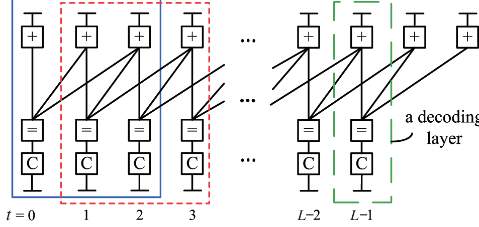
For convenience, the MI between the a priori input and the corresponding codeword bit is referred to as the a priori MI, the MI between the extrinsic output and the corresponding codeword bit is referred to as the extrinsic MI, and the MI between the channel observation and the corresponding codeword bit is referred to as the channel MI. The analysis assumes that the interleavers $\mbox{\boldmath$\varPi$\unboldmath}_{i}$ ($0\leq i\leq m$) are arbitrarily large and random.

BMST code ensembles can be represented by a Forney-style factor graph, also known as a normal graph [20], where edges represent variables and vertices (nodes) represent constraints. All edges connected to a node must satisfy the specific constraint of the node. A full-edge connects to two nodes, while a half-edge connects to only one node. A half-edge is also connected to a special symbol, called a “dongle”, that denotes coupling to other parts of the transmission system (say, the channel or the information source) [20]. There are three types of nodes in the normal graph of BMST codes.²² 2 For more details on the normal realization of BMST codes, we refer the reader to [11, 12].

• •

  Node +: All edges (variables) connected to node + must sum to zero. The message updating rule at node + is similar to that of the check node in the factor graph of a binary LDPC code. The only difference is that the messages on the half-edges are obtained from the channel observations.

• •

  Node =: All edges (variables) connected to node = must take the same (binary) value. The message updating rule at node = is the same as that of the variable node in the factor graph of a binary LDPC code.

• •

  Node C: All edges (variables) connected to node C must satisfy the constraint specified by the basic code. The message updating rule at node C can be derived accordingly, where the messages on the half-edges are associated with the information source.

The normal graph of a BMST code ensemble can be divided into layers, where each layer typically consists of a node of type C, a node of type =, and a node of type +. Similar to SC-LDPC codes, an iterative sliding window decoding EXIT chart analysis algorithm with decoding delay $d$ working over a subgraph consisting of $d+1$ consecutive layers can be implemented to study the convergence behavior of BMST codes.³³ 3 As with SC-LDPC codes, the decoding delay $d$ must be chosen several times as large as the encoding memory $m$ in order to achieve good performance. The first layer in any window is called the target layer. An example of a window decoder with decoding delay $d=2$ operating on the normal graph of a BMST code ensemble with $m=2$ is shown in Fig. 1. In our modified EXIT chart analysis, the convergence check at node C is performed as follows.

Given a channel parameter ${E_{b}}/{N_{0}}$, the channel MI is given by

The modified EXIT chart analysis algorithm of BMST codes can now be described as follows.

Now we can denote the iterative decoding threshold ${({E_{b}}/{N_{0}})}^{*}$ of BMST code ensembles for a preselected target BER as the minimum value of the channel parameter ${E_{b}}/{N_{0}}$ which allows the decoder of Algorithm 1 to output a decoding success, in the limit of large code lengths (i.e., $M\rightarrow\infty$).

References

- [1] A. J. Felström and K. S. Zigangirov, “Time-varying periodic convolutional codes with low-density parity-check matrix,” IEEE Trans. Inf. Theory, vol. 45, no. 6, pp. 2181–2191, Sept. 1999.
- [2] M. Lentmaier, A. Sridharan, D. J. Costello, Jr., and K. S. Zigangirov, “Iterative decoding threshold analysis for LDPC convolutional codes,” IEEE Trans. Inf. Theory, vol. 56, no. 10, pp. 5274–5289, Oct. 2010.
- [3] D. G. M. Mitchell, M. Lentmaier, and D. J. Costello, Jr., “Spatially coupled LDPC codes constructed from protographs,” 2014, submitted to IEEE Trans. Inf. Theory. [Online]. Available: http://arxiv.org/abs/1407.5366.
- [4] S. Kudekar, T. J. Richardson, and R. L. Urbanke, “Spatially coupled ensembles universally achieve capacity under belief propagation,” IEEE Trans. Inf. Theory, vol. 59, no. 12, pp. 7761–7813, Dec. 2013.
- [5] A. E. Pusane, R. Smarandache, P. O. Vontobel, and D. J. Costello, Jr., “Deriving good LDPC convolutional codes from LDPC block codes,” IEEE Trans. Inf. Theory, vol. 57, no. 2, pp. 835–857, Feb. 2011.
- [6] A. R. Iyengar, M. Papaleo, P. H. Siegel, J. K. Wolf, A. Vanelli-Coralli, and G. E. Corazza, “Windowed decoding of protograph-based LDPC convolutional codes over erasure channels,” IEEE Trans. Inf. Theory, vol. 58, no. 4, pp. 2303–2320, Apr. 2012.
- [7] I. Andriyanova and A. Graell i Amat, “Threshold saturation for nonbinary SC-LDPC codes on the binary erasure channel,” 2013, submitted to IEEE Trans. Inf. Theory. [Online]. Available: http://arxiv.org/abs/1311.2003
- [8] D. G. M. Mitchell, A. E. Pusane, and D. J. Costello, Jr., “Minimum distance and trapping set analysis of protograph-based LDPC convolutional codes,” IEEE Trans. Inf. Theory, vol. 59, no. 1, pp. 254–281, Jan. 2013.
- [9] L. Wei, D. G. M. Mitchell, T. E. Fuja, and D. J. Costello, Jr., “Design of spatially coupled LDPC codes over GF() for windowed decoding,” 2014, submitted to IEEE Trans. Inf. Theory. [Online]. Available: http://arxiv.org/abs/1411.4373
- [10] K. Huang, D. G. M. Mitchell, L. Wei, X. Ma, and D. J. Costello, Jr., “Performance comparison of LDPC block and spatially coupled codes over GF,” IEEE Trans. Commun., 2015, to appear.
- [11] X. Ma, C. Liang, K. Huang, and Q. Zhuang, “Block Markov superposition transmission: Construction of big convolutional codes from short codes,” 2013, submitted to IEEE Trans. Inf. Theory. [Online]. Available: http://arxiv.org/abs/1308.4809
- [12] C. Liang, X. Ma, Q. Zhuang, and B. Bai, “Spatial coupling of generator matrices: A general approach to design good codes at a target BER,” IEEE Trans. Commun., vol. 62, no. 12, pp. 4211–4219, Dec. 2014.
- [13] A. J. Feltström, D. Truhachev, M. Lentmaier, and K. S. Zigangirov, “Braided block codes,” IEEE Trans. Inf. Theory, vol. 55, no. 6, pp. 2640–2658, June 2009.
- [14] B. P. Smith, A. Farhood, A. Hunt, F. R. Kschischang, and J. Lodge, “Staircase codes: FEC for 100 Gb/s OTN,” J. Lightwave Technol., vol. 30, no. 1, pp. 110–117, Jan. 2012.
- [15] S. Moloudi, M. Lentmaier, and A. Graell i Amat, “Spatially coupled turbo codes,” in Proc. Int. Symp. Turbo Codes Iterative Inf. Process., Bremen, Germany, Aug. 2014.
- [16] A. Abbasfar, D. Divsalar, and K. Yao, “Accumulate-repeat-accumulate codes,” IEEE Trans. Commun., vol. 55, no. 4, pp. 692–702, Apr. 2007.
- [17] C. Liang, J. Hu, X. Ma, and B. Bai, “A new class of multiple-rate codes based on block Markov superposition transmission,” 2014, submitted to IEEE Trans. Signal Process. [Online]. Available: http://arxiv.org/abs/1406.2785
- [18] S. ten Brink, “Convergence behavior of iteratively decoded parallel concatenated codes,” IEEE Trans. Commun., vol. 49, no. 10, pp. 1727–1737, Oct. 2001.
- [19] G. Liva and M. Chiani, “Protograph LDPC codes design based on EXIT analysis,” in Proc. IEEE Global Commun. Conf., Washington, DC, Nov. 2007.
- [20] G. D. Forney Jr., “Codes on graphs: Normal realizations,” IEEE Trans. Inform. Theory, vol. 47, no. 2, pp. 520–548, Feb. 2001.
- [21] S. ten Brink, G. Kramer, and A. Ashikhmin, “Design of low-density parity-check codes for modulation and detection,” IEEE Trans. Commun., vol. 52, no. 4, pp. 670–678, Apr. 2004.