Scalar clouds in charged stringy black hole-mirror system
Abstract
It was reported that massive scalar fields can form bound states around Kerr black holes [C. Herdeiro, and E. Radu, Phys. Rev. Lett. 112, 221101 (2014)]. These bound states are called scalar clouds, which have a real frequency , where is the azimuthal index and is the horizon angular velocity of Kerr black hole. In this paper, we study scalar clouds in a spherically symmetric background, i.e. charged stringy black holes, with the mirror-like boundary condition. These bound states satisfy the superradiant critical frequency condition for charged scalar field, where is charge of scalar field, and is horizon electrostatic potential. We show that, for the specific set of black hole and scalar field parameters, the clouds are only possible for the specific mirror locations . It is shown that analytical results of mirror location for the clouds are perfectly coincide with numerical results in the regime. We also show that the scalar clouds are also possible when the mirror locations are close to the horizon. At last, we provide an analytical calculation of the specific mirror locations for the scalar clouds in the regime.
Keywords:
black hole, superradiance, scalar cloudpacs
04.70.-s, 04.60.CfI Introduction
It was firstly proposed by S. Hod that the scalar field can have real bound states in the near-extremal Kerr black hole [1, 2]. Soon later, it was reported in [3] that massive scalar fields can form bound states around Kerr black holes by using the numerical method to solve the scalar field equation in the background. This bound states are the stationary scalar configurations in the black hole backgrounds, which are regular at the horizon and outside. They are named as scalar clouds. More importantly, it was shown that the backreaction of clouds can generate a new family of Kerr black holes with scalar hair [3, 4]. It is suggested that whenever clouds of a given matter field can be found around a black hole, in a linear analysis, there exists a fully non-linear solution of new hairy black hole correspondingly. However, it requires that the field originating clouds yields a time independent energy momentum tensor. Generally, the field should be complex, and have a factor , where is the superradiance critical frequency. For instance, real scalar fields can give rise to clouds but not hairy black holes [5]. So, it seems that the studies of scalar clouds in the linear level are very important for us to find the hairy black holes in the non-linear level. This subject has attracted a lot of attention recently [6, 7, 8, 9, 10, 11, 12, 13, 14, 15, 16].
Generally speaking, the existence of stationary bound states of matter fields in the black hole backgrounds requires two necessary conditions. The first is that the matter fields should undergo the classical superradiant phenomenon [17, 18] in the black hole background. This condition can be satisfied by the bosonic fields in the rotating black holes or the charged scalar fields in the charged black holes [19]. When the frequencies of these matter fields are smaller than the superradiant critical frequency , there are time growing quasi-bound states. When , the fields are time decaying. So, the scalar clouds exists at the boundary between these two regimes, i.e. the frequencies of the fields are taken as the superradiant critical frequency . For the rotating black holes, the critical frequency is , where is the azimuthal index and is the horizon angular velocity. While for the charged black holes, , where is the charge of scalar field, and is the horizon electrostatic potential. The second one is there should be a potential well outside the black hole horizon in which the bound states can be trapped. This potential well may be provided by the mass term of the field, i.e. , where is the mass of the scalar field. However, sometimes the artificial boundary conditions can also play the same role.
In this paper, we will study the scalar clouds in a spherically symmetric and charged background. Specifically, we will consider the charged scalar field in the backgrounds of the charged stringy black holes. At first sight, it seems that the massive scalar field can form the clouds in this background. However, it is proved that the the massive charged scalar field is stable in this background and there is no superradiant instability [20]. To generate the superradiant instability [21], the mirror-like boundary condition should be imposed according to the black hole bomb mechanism [22, 23]. The analytical and the numerical studies on this subject can be found in [24] and [25]. Correspondingly, the scalar clouds are only possible with the mirror-like boundary condition. Using the numerical method, we will study the dynamics of the massless charged scalar field satisfying the frequency condition and the mirror-like boundary condition. We will show that, for the specific set of black hole and scalar field parameters, the clouds are only possible for the specific mirror locations . It will be shown that the analytical results of mirror location for the clouds are perfectly coincide with the numerical results. In addition, we will show that the scalar clouds are also possible when the mirror locations are close to the horizon. At last, we will provide an analytical calculation of the specific mirror locations for the scalar clouds in the regime.
This paper is organized as follows. In Sec.II, we will present the background geometry of charged string black hole and the dynamic equation of the scalar field. In particularly, we will give the superradiant condition and the boundary condition of this black hole-mirror system. In Sec.III, we describe the numerical procedure to solve the radial equation under the certain boundary condition. In this section, the numerical results are also illustrated. Some general discussion on the numerical results are also followed. In Sec. IV, an analytical calculation of the mirror radius for scalar clouds in regime is present. The conclusion is appeared in Sec. IV.
II Description of the system
We shall consider a massless charged scalar field minimally coupled to the charged stringy black hole with the mirror-like boundary condition. The black hole is a static spherical symmetric charged black holes in low energy effective theory of heterotic string theory in four dimensions, which is firstly found by Gibbons and Maeda in [26] and independently found by Garfinkle, Horowitz, and Strominger in [27] a few years later. The metric is given by
| (1) | |||||
and the electric potential and the dilaton field
| (2) | |||
| (3) |
The parameters and are the mass and the electric charge of the charged stringy black hole, respectively. The event horizon of black hole is located at . The area of the sphere approaches to zero when . Therefore, the sphere surface of the radius is singular. When , this singular surface is surrounded by the event horizon. In this paper, we will always assume the cosmic censorship hypothesis, i.e. we will only consider the black hole with the parameters satisfying the condition .
The dynamics of the charged scalar field is then governed by the Klein-Gordon equation
| (4) |
where denotes the charge of the scalar field. By taking the ansatz of the scalar field , where is the conserved energy of the mode, is the spherical harmonic index, and is the azimuthal harmonic index with , one can deduce the radial wave equation in the form of
| (5) |
where we have introduced a new function with and , and the potential function is given by
| (6) |
The superradiant condition of the charged scalar field is given by
| (7) |
where is the electric potential at the horizon[28, 20]. It is proved in [20] that the massive charged scalar field is stable in this black hole background. To have superradiant instability, we should impose the mirror-like boundary condition [24, 25]. In order to study the bound states, we shall focus on the critical case that the scalar frequency equals to the superradiant critical frequency, i.e.
| (8) |
To solve the radial equation (5), we should impose the following boundary conditions, which are given by
The first line indicates that the scalar field is regular near the horizon and the second line implies that the system is placed in a perfectly reflecting cavity.
III Numerical procedure and results
The numerical methods employed in this problem are based on the shooting method, which is also called the direct integration (DI) method [29, 30, 31, 32]. It is shown that the DI method is specially suited to find stationary field configuration with the mirror-like boundary condition.
Firstly, near the event horizon , we require the radial function is regular and expand the radial function as a generalized power series in terms of as have done in the first line of Eq.(9). Because the radial equation is linear, we can take without loss of generality. Substituting expansion of the radial wave function into the radial equation (5), we can solve the coefficient order by order in terms of . We have only considered six terms in the expansion. The s can be expressed in terms of the parameters , which are not exhibited here.
Then, we can integrate the radial equation (5) from and stop the integration at the radius of the mirror. In this procedure, we have taken the small as . The procedure can be repeated by varying the input parameters until the mirror-like boundary condition is reached with the desired precision. We can use a numerical root finder to search the location of the mirror that support the stationary scalar configuration. We have found that, for the given input parameters , scalar clouds exist for a discrete set of , which is labeled by the quantum number of nodes of the radial function .


Firstly, we make a comparison of the numerical and analytical results. From the analytical result Eq.(35) in Ref.[24], one can obtain the mirror radius that supports scalar cloud can be approximately given by
| (12) |
We have labeled the -th positive zero of the Bessel function as . The numerical results show that this ”quantum number” is closely connected with the nodes number of the radial function towards the simple relation . It should be noted that this analytical expression for the mirror radius is only valid for the case of . With the condition , the asymptotic expansion matched method can be employed to solve the radial equation approximately [24]. In Fig.(1), we have displayed the analytical results and the numerical results of the mirror location in terms of the black hole charge . Here, we do not consider the naked singularity spacetime, so that the value range of black hole charge is , where we have fixed the black hole mass as . It is shown that the analytical results of mirror location for the clouds are perfectly coincide with the numerical results, even in the region where the analytical approximation is unapplicable. When , the analytical approximation is always precise in all range of . When , the analytical results have obvious difference with the numerical results only for large .
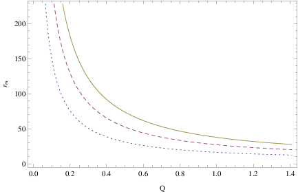
In Fig.(2), we have drawn the mirror location that support the scalar cloud as a function of the black hole charge for various values of node number of the radial function. It is observed that, when the black hole charge increases, we need to place the reflecting mirror more closer to the horizon in order to have a scalar cloud. When the node number of radial function increases, the plotted lines become away from the axis. This observation is coincide with the analytical result (10) in the regime of .
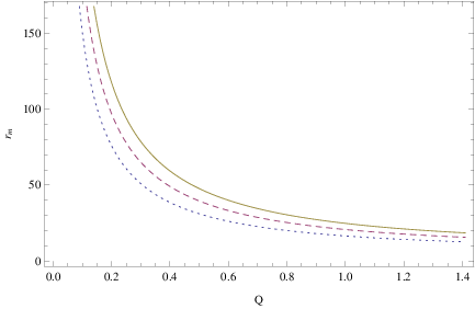
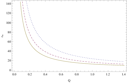
In Fig.(3) and (4), we display the mirror location as a function of the black hole charge for various different and . We can observe that, the lines become far away from the axis when increasing , while the lines become more closer to the axis when increasing the scalar charge . This is also expected from the analytical result (10). In addition, Fig.(3) and (4) together with Fig.(2) show that, when , . This indicates that there is no massless scalar cloud for Schwarzschild black hole with the mirror-like boundary condition [16], even thought it is possible for massive scalar fields in Schwarzschild black hole to have arbitrarily long-lived quasi-bound states [33].


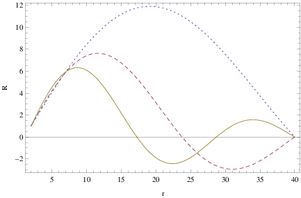
We also consider the radial dependence of the massless scalar clouds. In Fig.(5) and (6), we have fixed the mirror radius as . We can solve the radial equation numerically and obtain a discrete set of black hole charge which is labeled by the node number of the radial wave equation. Then we can integrate the radial equation for the fixed node numbers and obtain the corresponding numerical solutions of the radial wave functions. It is shown that the radial profile have the typical forms of standing waves with the fixed boundary conditions. We have also calculated the case that . The results is not present here. The general form of the radial wave function is similar to the profiles in Fig.(5).
In Fig.(7), we consider the case that the mirror location is very close to the horizon. We take the mirror radius as . From our previous analytical and numerical work on the superradiant instability of scalar field in the background of the charged stringy black hole plus mirror system, we need a large scalar field charge . Here, we set . We can see that, the scalar field can be bounded by the reflecting mirror very near the horizon to form the clouds. The radial wave function in this case have the similar profiles as Fig.(5) and (6).

IV Scalar clouds in regime
In the above numerical calculations, we find the radial equation becomes hard to integrate when the scalar charge is large. So it is important to make an analytical study of the stationary charged scalar clouds in the regime. In this section, we will give an analytical expression of special mirror radius in limit, for which the charged scalar field can be confined to form stationary cloud configuration.
Following [34], it is convenient to introduce new dimensionless variables
| (13) |
in terms of which the radial equation (5) becomes
| (14) |
where we have submit the superradiance critical frequency in the above equation.
This equation can be solved by Bessel function in the double limit
| (15) |
In this asymptotic regime, the radial equation can be reduced to
| (16) |
The solution is then given by the Bessel function of the first kind
| (17) |
i.e., the stationary scalar field is then described by the above function. By taking account to the mirror-like boundary condition , we can obtain the special mirror radius as
| (18) |
where is the th positive zero of the Bessel function . From this expression, we can see that, when , the reflecting mirror should be placed very near the horizon to form the cloud configuration. This is consistent with the near horizon condition .
V Conclusion
In summary, in this paper, we have studied the massless scalar clouds in the charged stringy black holes with the mirror-like boundary conditions. The scalar clouds are stationary bound states satisfying the superradiant critical frequency . The scalar clouds in rotating black holes [3, 8] can be heuristically interpreted in terms of a mechanical equilibrium between the Black hole-cloud gravitational attraction and angular momentum driven repulsion. For the charged black hole cases, the charged clouds can not be formed because gravitational attraction and electromagnetic repulsion can not reach equilibrium [7]. Additional mirror should be placed at special location to reflect the charged scalar wave.
We show that, for the specific set of black hole and scalar field parameters, the clouds are only possible for the specific mirror location . For example, for the fixed parameters of black hole and scalar field , the discrete set of the mirror location is characterized by the node number of the radial wave function. It is shown that, the analytical results of mirror location for the clouds are perfectly coincide with the numerical results in the region of . However, the agreement becomes less impressive for values. In addition, we also show that the massless scalar clouds are also possible when the mirror locations are very close to the horizon. At last, we present an analytical calculation of the specific mirror locations for the scalar clouds in the regime.
ACKNOWLEDGEMENT
The authors would like to thank Dr. Hongbao Zhang for useful discussion on the numerical methods. This work was supported by NSFC, China (Grant No. 11205048).
References
- [1] S. Hod, Phys. Rev. D 80, 104026 (2012).
- [2] S. Hod, Eur. Phys. J. C 73, 2378 (2013).
- [3] C. A. R. Herdeiro, and E. Radu, Phys. Rev. Lett. 112, 221101 (2014).
- [4] C. A. R. Herdeiro, and E. Radu, Phys. Rev. D 89, 124018 (2014).
- [5] C. Herdeiro, and E. Radu, arXiv:1501.04319[gr-qr].
- [6] S. Hod, Phys. Rev. D 90, 024051 (2014).
- [7] J. Degollado, and C. Herdeiro, Gen. Rel. Grav. 45, 2483 (2013).
- [8] C. Benone, L. Crispino, C. Herdeiro, and E. Radu, Phys. Rev. D 90, 104024 (2014).
- [9] M. Sampaio, C. Herdeiro, and M. Wang, Phys. Rev. D 90, 064004 (2014).
- [10] A. Graham, and R. Jha, Phys. Rev. D 90, 041501 (2014).
- [11] J. Degollado, and C. Herdeiro, Phys. Rev. D 90, 065019 (2014).
- [12] Y. Brihaye, C. Herdeiro, and Eugen Radu, Phys. Lett. B 739, 1 (2014).
- [13] C. Herdeiro, E. Radu, and H. Runarsson, Phys. Lett. B 739, 302 (2014).
- [14] S. Hod, Phys. Lett. B 739, 196 (2014).
- [15] S. Hod, Phys. Lett. B 736, 398 (2014).
- [16] C. Benone, L. Crispino, C. Herdeiro, and E. Radu, arxiv: 1412.7278 [gr-qc].
- [17] J. M. Bardeen, W. H. Press, and S. A. Teukolsky, Astrophys. J. 178, 347 (1972).
- [18] C. W. Misner, Bull. Am. Phys. Soc. 17, 472 (1972).
- [19] J.D. Bekenstein, Phys. Rev. D 7, 949 (1973).
- [20] R. Li, Phys. Rev. D 88, 127901 (2013).
- [21] S. Detweiler, Phys. Rev. D 22, 2323 (1980); H. Furuhashi and Y. Nambu, Prog. Theor. Phys. 112, 983 (2004).
- [22] W. H. Press, and S. A. Teukolsky, Nature (London) 238, 211 (1972).
- [23] V. Cardoso, O. J. C. Dias, J. P. S. Lemos, and S. Yoshida, Phys. Rev. D 70, 044039 (2004).
- [24] R. Li, and J. Zhao, Eur. Phys. J. C 74, 3051(2014).
- [25] R. Li, and J. Zhao, Phys. Lett. B 740, 317 (2015).
- [26] G. W. Gibbons, and K. Maeda, Nucl. Phys. B 298, 741 (1998).
- [27] D. Garfinkle, G. T. Horowitz, and A. Strominger, Phys. Rev. D 43, 3140 (1991).
- [28] K. Shiraishi, Mod. Phys. Lett. A 7, 3449 (1992); J. Koga and K. Maeda, Phys. Lett. B 340, 29 (1994).
- [29] J. C. Degollado, C. A. R. Herdeiro, and H. F. Runarsson, Phys. Rev. D 88, 063003 (2013).
- [30] S. R. Dolan, L. A. Oliveira, and L. C. B. Crispino, Phys. Rev. D 82, 084037(2010).
- [31] L. A. Oliveira, V. Cardoso, and L. C. B. Crispino, Phys. Rev. D 89, 124008(2014).
- [32] N. Uchikata, S. Yoshida, and T. Futamase, Phys. Rev. D 80, 084020(2009).
- [33] J. Barranco, et.al. Phys. Rev. Lett. 109, 081102 (2012).
- [34] S. Hod, Phys. Rev. D 88, 064055 (2013).