Partial covering of emission regions of Q 0528 $-$ 250 by intervening H₂ clouds.

Partial covering of emission regions of Q 0528

-

250 by intervening H₂ clouds.–202015

V.V. Klimenko Affiliation: Ioffe Physical-Technical Institute of RAS, Polyteknicheskaya 26, 194021 Saint-Petersburg, Russia Affiliation: St.-Petersburg State Polytechnical University, Polyteknicheskaya 29, 195251 Saint-Petersburg, Russia S.A. Balashev Affiliation: Ioffe Physical-Technical Institute of RAS, Polyteknicheskaya 26, 194021 Saint-Petersburg, Russia Affiliation: St.-Petersburg State Polytechnical University, Polyteknicheskaya 29, 195251 Saint-Petersburg, Russia A.V. Ivanchik Affiliation: Ioffe Physical-Technical Institute of RAS, Polyteknicheskaya 26, 194021 Saint-Petersburg, Russia Affiliation: St.-Petersburg State Polytechnical University, Polyteknicheskaya 29, 195251 Saint-Petersburg, Russia C. Ledoux Affiliation: European Southern Observatory, Alonso de Córdova 3107, Casilla 19001, Vitacura, Santiago 19, Chile P. Noterdaeme Affiliation: Université Pierre et Marie-Curie, Institut d’Astrophysique de Paris, CNRS-UMR7095, 98bis boulevard Arago, 75014 Paris, France P. Petitjean Affiliation: Université Pierre et Marie-Curie, Institut d’Astrophysique de Paris, CNRS-UMR7095, 98bis boulevard Arago, 75014 Paris, France R. Srianand Affiliation: Inter-University Centre for Astronomy and Astrophysics, Post Bag 4, Ganesh Khind, Pune 411 007, India D.A. Varshalovich Affiliation: Ioffe Physical-Technical Institute of RAS, Polyteknicheskaya 26, 194021 Saint-Petersburg, Russia Affiliation: St.-Petersburg State Polytechnical University, Polyteknicheskaya 29, 195251 Saint-Petersburg, Russia

Accepted 15.12.2014 Received 08.10.2014

Abstract

We present an analysis of the molecular hydrogen absorption system at $z_{abs}=2.811$ in the spectrum of the blazar Q 0528 $-$ 250. We demonstrate that the molecular cloud does not cover the background source completely. The partial coverage reveals itself as a residual flux in the bottom of saturated H₂ absorption lines. This amounts to about $(2.22\pm 0.54)\%$ of the continuum and does not depend on the wavelength. This value is small and it explains why this effect has not been detected in previous studies of this quasar spectrum. However, it is robustly detected and significantly higher than the zero flux level in the bottom of saturated lines of the Ly $\alpha$ forest, $(-0.21\pm 0.22)$ per cent. The presence of the residual flux could be caused by unresolved quasar multicomponents, by light scattered by dust, and/or by jet-cloud interaction. The H₂ absorption system is very well described by a two-component model without inclusion of additional components when we take partial coverage into account. The derived total column densities in the H₂ absorption components A and B are $\log N({\rm H}_{2})[{\rm cm^{-2}}]=18.10\pm 0.02$ and 17.82 $\pm$ 0.02, respectively. HD molecules are present only in component B. Given the column density, $\log N{\rm(HD)}=13.33\,\pm\,0.02$ , we find $N({\rm{HD}})/\,2N(\rm{H_{2}})\,=\,(1.48\,\pm\,0.10)\,\times\,10^{-5}$ , significantly lower than previous estimations. We argue that it is crucial to take into account the partial coverage effects in any analysis of H₂ bearing absorption systems, in particular when studying the physical state of high-redshift interstellar medium.

Keywords:

cosmology:observations, ISM:clouds, quasar:individual:Q 0528

-

250

1 Introduction

As a result of their cosmological distances quasars (QSOs) appear as point-like objects. Various studies have aimed to explore the detailed inner structure of quasars, which is unresolved even for low-redshift active galactic nuclei (AGNs), because of their remote distances and sub-parsec scales of their emission regions. In the standard AGN paradigm the central region is divided into an accretion disk, a dusty-torus, a jet, a broad line region (BLR), and a narrow line region (NLR). Each of these regions contribute differently to the AGN emission spectrum.

Direct imaging of the spatial structure of AGNs is possible with current instruments mainly probing longer scales. To date, several interferometric studies of the central engine of the brightest AGNs (e.g. Jaffe et al. 2004; Tristram et al. 2014; López-Gonzaga et al. 2014) have revealed the existence of a hot, parsec-scale disk that is surrounded by warm dust extended in the polar direction. In the optical band the geometry of the emission line region is investigated by indirect methods. Reverberation mapping establishes the relationship between the size and the luminosity of the BLR and yields a typical BLR size of ${\rm R}_{\rm BLR}\sim$ 0.2 pc (Kaspi et al., 2007; Chelouche & Daniel, 2012) for high redshift luminous quasars. Differential microlensing allows for a constraint on the accretion disk size $\;\raise 1.29167pt\hbox{$<$\kern-7.5pt\raise-4.73611pt\hbox{$\sim$}}\;3\times 10^{-3}$ pc (Blackburne et al., 2011; Jiménez-Vicente et al., 2012) and for an estimation of the size of the BLR $\sim 0.1$ pc (Sluse et al., 2011). The observations of gamma-ray emission constrain the size of a jet constituent to a few parsecs (Abdo et al., 2010).

Another estimate of the size of the AGN emitting regions comes from constraints derived from covering factor analysis of intervening H₂ bearing clouds which happen to cover the background source only partially. Analysis of the partial coverage of Q 1232 $+$ 082 by a molecular hydrogen absorption cloud allowed Balashev et al. (2011) to estimate the size of the C IV BLR, R ${}_{\mbox{\small C\,{\sc IV}}}\sim\,0.16^{+0.08}_{-0.11}$ pc.

Molecular hydrogen absorption systems, a subset of damped Ly $\alpha$ systems (DLAs) and sub-damped Ly $\alpha$ systems (sub-DLAs), reveal diffuse and translucent interstellar clouds in high redshift intervening galaxies (Noterdaeme et al., 2008). An analysis of H₂ absorption systems allows for examining the physical conditions of diffuse clouds in distant galaxies (Srianand et al., 2005; Noterdaeme et al., 2007). It has been shown that the gas is a part of the cold neutral medium with comparatively low kinetic temperature ( $T\sim 50-500\,$ K) and high densities ( $n_{\rm H}$ $>$ 10 cm^-3), thus compact sizes ( $l\;\raise 1.29167pt\hbox{$<$\kern-7.5pt\raise-4.73611pt\hbox{$\sim$}}\;1\,$ pc). Comparison of 21 cm and H₂ absorptions suggests that the H₂ absorption originates from a compact gas that probably contains only a small fraction of H i measured along the line of sight (Srianand et al., 2012). These systems are important instruments for the analysis of several cosmological problems, as follows. (i) The discovery of HD/H₂ clouds at high redshift (Varshalovich et al., 2001) provides an independent way to estimate the primordial deuterium abundance (D/H) and therefore the relative baryon density of the Universe $\Omega_{\rm b}$ which is one of the key cosmological parameters (Balashev et al., 2010; Ivanchik et al., 2010). (ii) The comparison of H₂ wavelengths observed in QSO spectra with laboratory ones (just for this quasar Q 0528 $-$ 250, Varshalovich & Levshakov (1993), Cowie & Songaila (1995), Potekhin et al. (1998), Ubachs & Reinhold (2004), King et al. (2011)) allows us to test the possible cosmological variation of the proton-to-electron mass ratio $\mu=m_{p}/m_{e}$ . Because the de-composition of H₂ absorptions into several components is crucial for studies of the fundamental constant variability problem, we should pay attention to the partial coverage effect. It is known that taking into account the partial coverage effects, the physical model of the absorption system differs (see Balashev et al. 2011). (iii) The interpretation of the relative populations of C i fine-structure excitation levels and CO rotational levels (Srianand et al. 2000; Noterdaeme et al. 2011) allows us to measure the temperature $T_{\rm CMB}(z)$ of the cosmic microwave background radiation at high redshift.

Here, we argue that it is necessary to take into account the partial coverage of quasar emission regions by a compact intervening H₂ cloud in order to derive a robust fit of the absorption lines. If this effect is not taken into account, column densities can be underestimated by a factor of up to two orders of magnitude. The first case of such an analysis has been presented by Balashev et al. 2011 for Q 1232 $+$ 082. The second case of partial coverage has been detected by Albornoz Vásquez et al. (2014) for H₂ bearing cloud towards the quasar Q 0643 $-$ 504. The third case of partial coverage for the H₂ cloud at $z_{\rm abs}=2.811$ in the spectrum of Q 0528 $-$ 2508 is presented in this study. We analyse a new spectrum and detect residual flux in the bottom of saturated H₂ lines ( ${\rm J=0}$ and ${\rm J=1}$ levels). In case this flux is not taken into account, saturated lines yield large $\chi^{2}$ values and a multicomponent model is used instead (e.g. King et al. 2011).

The remainder of this paper is organized as follows. A brief description of the data is given in Section 2. The principles of partial coverage are described in Section 3. In Section 4, we present the analysis of the H₂ absorption system, accounting for partial coverage . The HD molecular lines are explored in Section 5. The results are discussed in Section 6, and we give a brief conclusion in Section 7.

2 Data

The molecular hydrogen was identified for the first time at high redshift in the very spectrum of Q 0528 $-$ 2508 (Levshakov & Varshalovich, 1985). This quasar was observed many times, in particular during the period between 2001 and 2009 using both spectroscopic arms of Ultraviolet and Visual Echelle Spectrograph (UVES) of the Very Large Telescope (VLT); for a description of the instrument, see Dekker et al. (2000). The log of the observations used in our work is shown in Table 1. These observations relate to four programmes, three of which were carried out in 2001–2002: 66.A-0594(A) (PI: Molaro), 68.A-0600(A) (PI: Ledoux), and 68.A-0106(A) (PI: Petitjean). The instrument settings used during these observations were a 1-arcsec slit and 2x2 CCD pixel binning in both arms, resulting in a resolving power of R $\sim$ 45000 in the blue and R $\sim$ 43000 in the red. There was no ThAr lamp calibration attached to each of the exposures. An additional series of observations was performed in 2008-2009 under programme 082.A-0087(A) (PI: Ubachs). The settings for that programme were a 0.8-arcsec slit in the blue arm and a 0.7-arcsec slit in the red. The 2x2 CCD pixel binning was also used at that time. This resulted in a resolving power of R $\sim$ 60000 in the blue and R $\sim$ 56000 in the red. Because the goal of that programme was to set a limit on the variation of $\mu$ , ThAr lamp calibrations were also taken immediately after each observation.

The data presented in Table 1 were reduced using the UVES Common Pipeline Library (CPL) data reduction pipeline release 4.9.5 using the optimal extraction method¹¹ 1 see the UVES pipeline user manual available for download at ftp://ftp.eso.org/pub/dfs/pipelines/uves/uves-pipeline-manual-22.8.pdf. The inter-order background (scattered light inside the instrument) was carefully subtracted in both the flat-field frames and the science exposures. Linear spline interpolation was used to produce a two-dimensional background image, which was subsequently smoothed using an average boxcar. Fourth-order polynomials were used to find the dispersion solutions. However, the errors only reflect the calibration error at the observed wavelengths of the ThAr lines used for wavelength calibration. All the spectra were corrected for the motion of the observatory around the barycentre of the Solar system and then converted to vacuum wavelengths. These spectra were interpolated into a common wavelength array and generated the weighted-mean combined spectrum using the inverse squares of errors as weights. All the available exposures were utilized to increase the signal-to-noise ratio up to $\sim$ 60 per pixel in the wavelength range of the H₂ absorption lines (at $z=2.811$ ). As shown below, this allows us to detect and study the effect of partial coverage in details.

Table 1: Log of the observations

No.	UT Date	Program ID	Exposure	Slit
			(sec)	(arcsec)
1	03.02.2001	66.A-0594(A)	1 $\times$ 5655	1.0
2	04.02.2001	66.A-0594(A)	2 $\times$ 5655	1.0
3	05.02.2001	66.A-0594(A)	1 $\times$ 5655	1.0
4	07.02.2001	66.A-0594(A)	1 $\times$ 5655	1.0
5	13.02.2001	66.A-0594(A)	1 $\times$ 5655	1.0
6	13.03.2001	66.A-0594(A)	1 $\times$ 5655	1.0
7	15.03.2001	66.A-0594(A)	1 $\times$ 5655	1.0
8	17.10.2001	68.A-0600(A)	1 $\times$ 3600	1.0
9	18.10.2001	68.A-0600(A)	2 $\times$ 3600	1.0
10	08.01.2002	68.A-0106(A)	2 $\times$ 3600	1.0
11	09.01.2002	68.A-0106(A)	2 $\times$ 3600	1.0
12	10.01.2002	68.A-0106(A)	2 $\times$ 3600	1.0
13	23.11.2008	082.A-0087(A)	2 $\times$ 2900	0.8-0.7
14	25.11.2008	082.A-0087(A)	1 $\times$ 2900	0.8-0.7
15	23.12.2008	082.A-0087(A)	4 $\times$ 2900	0.8-0.7
16	25.01.2009	082.A-0087(A)	1 $\times$ 2900	0.8-0.7
17	26.01.2009	082.A-0087(A)	1 $\times$ 2900	0.8-0.7
18	26.02.2009	082.A-0087(A)	1 $\times$ 2900	0.8-0.7
Total			108450

3 Effect of partial covering

Partial covering implies that only a part of the background source is covered by the absorbing cloud. Mainly this can be a consequence of the absorbing cloud size being comparable to, or even smaller than, the projected extent of the background source.

Refer to caption — Figure 1: An illustration of the effect of partial coverage on the absorption-line profiles. Different panels show (a) a highly saturated line with total coverage, $f_{\rm c}=1\,$ , (b) a highly saturated line with partial coverage, $f_{\rm c}=0.8\,$ and (c) a partially saturated line with the same partial coverage, $f_{\rm c}=0.8\,$ . The line flux residual (LFR) is the fraction of the QSO flux that is not intercepted by the cloud. It can be easily derived from the spectral analysis in case (b), but it is not straightforward to detect in case (c).

Partial covering is readily detectable in the spectrum of a background quasar if the cores of the saturated absorption lines do not reach the zero flux level. This indicates that a part of the radiation from the QSO passes by the cloud. The covering factor characterizing partial coverage is defined by the ratio,

f_{\rm c}=\frac{F_{\rm cloud}}{F_{\rm total}},

(1)

where $F_{\rm cloud}$ is the flux that passes through the absorbing gas and $F_{\rm total}$ is the total flux. Therefore the measured flux in the spectrum, $F(\lambda)$ , can be written as:

F(\lambda)=[F_{\rm total}(\lambda)-F_{\rm cloud}(\lambda)]+F_{\rm cloud}(\lambda)\exp[-\tau(\lambda)],

(2)

here $\,\tau(\lambda)\,$ is the optical depth of the cloud at the wavelength $\lambda$ . The line flux residual (LFR) is the fraction of the QSO flux which is not covered by the cloud. These definitions are illustrated in Fig. 1. The determination of the covering factor is trivial in the case of highly saturated absorption lines (see Fig. 1 panels (a) and (b)) while for a partially saturated line (see Fig. 1 case (c)) the analysis requires a more sophisticated procedure. In this case it is necessary to use several absorption lines originating from the same levels but with different values of $\lambda f$ , which is the product of the oscillator strength, $f$ , and the wavelength of the transition, $\lambda$ . Such an analysis has been performed by Ivanchik et al. (2010) and more precisely by Balashev et al. (2011) for the spectrum of Q 1232 $+$ 082, and by Albornoz Vásquez et al. (2014) for the spectrum of Q 0643 $-$ 504. A similar situation was observed for HE0001 $-$ 2340. Jones et al. (2010) have considered the possibility of partial coverage of the BLR to explain the observed Mg ii equivalent widths. In contrast to the rare situations where partial covering occurs from intervening systems (see also Petitjean et al. 2000), partial covering is typical for absorption systems associated with quasars ( e.g. Petitjean et al. 1994; Rupke et al. 2005; Hamann et al. 2010; Muzahid et al. 2013).

A failure to take into account the partial coverage effect in a spectroscopic analysis can lead to a significant underestimation of the column density of an absorber. The systematic bias (of column density) can exceed several orders of magnitude for saturated lines. As an example, consider an absorption line which consists of one component and has the high column density. The spectrum and the corresponding one-component model are shown in panel (a) of Fig. 2. In panels (b), (c), (d) and (e) the same line is presented, but part of radiation from background source (10 % for clarity) passes by a cloud. If we take into account the LFR, then the line can be properly fitted by a one component model and we can recover the high input column density (with given accuracy) and measure the LFR value (panel (e) of Fig. 2). If the residual flux is not taken into account, then the one component model – Lorentzian (b) or Gaussian (c) profiles – is not adequate, the reason being that a one-component Voigt profile cannot describe the unsaturated bottom and far wings of the line simultaneously. Using additional components, as shown in panel (d), a result with a satisfactory $\chi^{2}$ is obtained. However, this solution is incorrect, because the resulting column density ( $\log N=15.8$ ) is much smaller than the input one ( $\log N=18.2$ ). To distinguish between cases (d) and (e) we propose a new method based on an analysis of several absorption lines with different oscillator strengths. The description of the method and application to the analysis of H₂ in Q 0528 $-$ 250 are described in more detail later.

4 Molecular hydrogen

Molecular hydrogen lines are detected in the spectrum of Q 0528 $-$ 250 from the DLA at ${\rm z_{abs}=2.811}$ . Column density of neutral hydrogen in this DLA system is $\log N(\mbox{H\,{\sc i}})=21.35\pm 0.07$ (Noterdaeme et al., 2008). H₂ lines correspond to transitions from rotational levels up to ${\rm J=5}$ . To fit the molecular hydrogen lines, the spectrum has been normalized with a continuum constructed by fitting the selected continuum regions devoid of any absorptions with spline.

4.1 Number of components

Table 2: Results of the previous analyses of the H₂ system at

z=2.811

towards Q 0528

-

250.

Year	$\log N_{\rm tot}$	${\rm N_{Comp.}}$	Resolution	Ref.
1985	16.46 $\pm$ 0.07	1		[1]
1988	18.0	1	10 000	[2]
1998	16.77 $\pm$ 0.09	1	10 000	[3]
2005	18.22 ${}^{+0.13}_{-0.17}$	2	40 000	[4]
2006	18.45 $\pm$ 0.02	–		[5]
2011	16.56 $\pm$ 0.02	3	45 000	[6]
2015	18.28 $\pm$ 0.02	2	45 000	This work
[1] Levshakov & Varshalovich (1985); [2] Foltz et al. (1988);
[3] Srianand & Petitjean (1998); [4] Srianand et al. (2005);
[5] Ćirković et al. (2006); [6] King et al. (2011)

The profiles of the H₂ absorption lines have a complex structure that cannot be fitted with a single component. At least two components are clearly seen in the lines corresponding to ${\rm J=4,J=5}$ rotational levels (see Fig.3). Since the first identification of the H₂ system in the quasar (Levshakov & Varshalovich, 1985) other studies have been conducted, providing discordant results (see Table 2). Srianand et al. (2005) used a two-component model, while King et al. (2011) pointed out that a three-component model is very strongly preferred over two-component model. King et al. (2011) used a fitting procedure where they increased the number of components in the absorption system in order to minimize the corrected Akaike information criterion, AICC²² 2 This statistical criteria allows for a choice of prefered model among several models with different numbers of fitting parameters. ${\rm AICC}=\chi^{2}+2p+\frac{2p(p+1)}{n-p-1},$ where $p$ is the number of fitting parameters, $n$ is the number of spectral points, included in an analysis. (Sugiura, 1978; King et al., 2011). The resulting total column density differs by two order of magnitude from Srianand et al. (2005). In that case a criterion for choosing preferred model is the consistent derived physical parameters of a cloud. It can be noted note that by using H₂ column density reported by King et al. (2011) (based on the three-component model) a $N{\rm{(HD)}}/2N{\rm{(H_{2})}}$ ratio is obtained, that is about an order of magnitude higher than the primordial one. Meanwhile, the H₂ column density in two-component model of Srianand et al. (2005) gives a reasonable $N{\rm{(HD)}}/2N{\rm{(H_{2})}}$ ratio, which is consistent with the typical values measured at high redshift (Balashev et al., 2010).

A very important point for the choice of a reasonable absorption profile model in the case of Q 0528 $-$ 250 is the presence of Lorentzian wings in ${\rm J=0}$ , ${\rm J=1}$ line profiles (see Fig. 4). It is an indicator of the high H₂ column density of absorption system with $\log N{\rm(H_{2})>18}$ which is consistent with the result reported by Srianand et al. (2005). However, in the new spectrum of Q 0528 $-$ 250 the H₂ lines with prominent Lorentzian wings have some residual flux at the bottom which significantly differs from the zero flux level (see Fig. 4 and Fig. 5). As a consequence, the fit by Srianand et al. (2005) gives the large reduced $\chi^{2}$ . It is probable that the signal-to-noise ratio in the previous spectrum was insufficient to detect the residual flux.

The current study shows that the residual flux detected in the bottom of saturated H₂ lines in the spectrum of Q 0528 $-$ 250 is the result of a partial coverage effect. In this case, the profiles of H₂ lines can be very well fitted by two-component model. Therefore, there is no need to increase the number of components in H₂ profiles (such as it is done by King et al. 2011) to explain the complex structure of lines (an example is given in Fig. 2). In the next three subsections, we provide evidence of the existence of the partial coverage in the spectrum of Q 0528 $-$ 250.

4.2 Zero-flux level correction

To measure the LFR in H₂ absorption lines we need to derive the zero flux level in the spectrum. A non-zero flux in the core of a saturated absorption line can be the result of inaccurate determination in between spectral orders of scattered light inside the instrument. The zero flux level in the spectrum can be estimated using the saturated Ly $\alpha$ absorption lines which are numerous and almost uniformly distributed over the wavelength range where H₂ absorption lines are located. Ly $\alpha$ lines are associated with intergalactic clouds that are larger than several kpc, thus it is most likely that they cover the background source completely.

Wide flat bottom lines ( $\Delta\lambda>1$ Å, i.e. $\delta v>80$ km s^-1) were selected, which guarantees that lines are saturated and therefore measured fluxes in the bottom of the lines (LFRs) are the real zero flux level in the spectrum. These lines were selected in the spectral region 3500 $-$ 4700 Å. To estimate the residual flux at the bottom of the line the procedure illustrated in Fig. 6 was implemented. We selected several pixels in a line profile for which flux is within $f_{c}\pm 1\sigma_{i}$ , where $f_{c}$ is the flux at the centre of the line and $\sigma_{i}$ is the error in pixel $i$ . The residual flux was calculated as the median of the flux in the selected pixels. The width of the line bottom was estimated as the difference between the right most and left-most selected pixels from the line centre (see Fig. 6). The top-left panel of Fig. 5 shows the LFR values obtained for the selected saturated Ly $\alpha$ absorption lines. The average value is found to be $(-0.21\pm 0.04)\%$ . The standard deviation of the points is $\sigma\simeq 0.22\%$ . The green stars show the LFR values measured at the bottom of the Ly $\alpha$ and Ly $\beta$ lines associated with the DLA-system at ${\rm z_{abs}=2.79}$ and with the Ly $\alpha$ line of the second DLA-system at ${\rm z_{abs}=2.14}$ . These lines are the most saturated lines for the spectrum.

4.3 Partial coverage of H₂ absorption lines

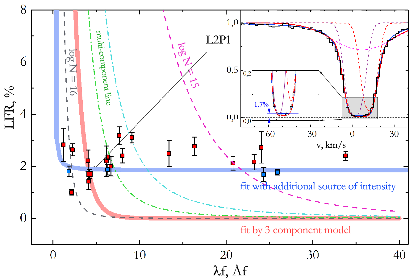
To estimate the residual flux in H₂ lines we selected ${\rm J=0,1}$ lines without apparent blends. The LFR was measured by the same technique as for the Ly $\alpha$ forest lines. The analysis found that the flux in the bottom of the lines is quite constant over large velocity range $\delta v\simeq 10$ km s^-1 (i.e. the dispersion of points is within the range of the average statistical error) that is wider than the full width half maximum (FWHM) of the UVES (6 km s^-1) and is comparable with the shift between centres of the two components. Therefore, the structure of H₂ system has no effect on the residual flux. The comparison of the obtained residual flux in the ${\rm J=0,1}$ H₂ lines with the level of the residual flux in the Ly $\alpha$ forest lines is shown in Fig.5. The filled squares represent the residual flux in H₂ lines versus its location in the spectrum. We have estimated the line flux residual at the level $2.22\pm 0.54$ % of the continuum, which significantly exceeds the zero-flux level.

Non-zero residual flux at the bottom of saturated lines can also be the result of the convolution of the saturated lines with the instrumental function, or an imperfect data reduction, and/or of the blend of several unresolved unsaturated lines. First, however H₂ lines are wide with widths larger than the FWHM of the UVES spectrograph (6 km/s, i.e. $\sim 0.08$ Å), so after convolution with the instrument function, the flux at the bottom of these lines must still go to zero. Secondly, the improper data reduction is not a viable explanation of the residual fluxes of saturated Ly $\alpha$ lines are consistently equal to zero. Also we tested the dependence of residual flux on the width of the bottom of line for H₂ and for the Ly $\alpha$ forest lines. This is shown in Fig.12. Several lines in the Ly $\alpha$ forest were detected; these have similar widths as the H₂ lines and go to the zero level. The profiles of these lines are shown in Fig. 13.

Lastly, the residual flux can not be a result of the composition of several unresolved unsaturated lines because the lines have Lorentzian wings.

4.3.1 The $\lambda f$ test

An additional test which confirms the presence of the partial coverage effect is discussed here (and illustrated in Fig. 7). Molecular hydrogen lines from ${\rm J=0,1}$ levels have very different values of the product $\lambda f$ (from 0.6 for L0P1 to 36.0 for W1Q1). It is known that the flux in the bottom of an absorption line decreases exponentially when $\lambda f$ increases, $F\propto\exp(-\lambda f)$ . The results of the calculation of this dependence for an absorption line in the spectrum with VLT resolution ( ${\rm FWHM=6\,km\,s^{-1}}$ ) are shown in Fig. 7 by the dashed lines. For simplicity, the modeled line profile consists of one component. The Doppler parameter ${\rm b=4\,km\,s^{-1}}$ and the Damping width $\Gamma_{lm}$ is the same as for the H₂ line L2P1. Because the equivalent width of the line gets to the logarithmic part of the curve of growth, we do not consider the different Doppler parameters. Two dashed curves (violet and grey) are calculated for the line with column densities $\log N=15$ and 16. The curve is shifted from right to left as the column density $N$ increases. For a higher column density, the residual flux equals zero for a wide range of $\lambda f$ (because the line is saturated) and differs from zero only for small values of $\lambda f\leq 5$ (the case of an unsaturated line). In a case of a multicomponent line (i.e. the blend of two or three lines with small column density $\log N=15$ ), the residual flux in the bottom of the blended line would also behave exponentially (dashed-dot curves). However, the behavior of the residual fluxes in the bottom of the saturated H₂ lines in the spectrum of Q 0528 $-$ 250 is quite different. The residual fluxes in the H₂ lines are shown by the filled blue and red squares. The squares do not follow the expected behavior, moreover the points scatter similarly around a median value in the whole range of $\lambda f$ .

Two models were applied to obtain a consistent and correct fit to the H₂ lines. Model (i) considers the best fit of the certain H₂ line (e.g. L2P1), which has a value of $\lambda f$ = 4.23 and ${\rm LFR=1.7\,\%}$ of the total flux. The line has a wide flat bottom $(\delta v\sim 10\,{\rm km\,s^{-1}})$ and Lorentzian wings. To fit this line without the partial coverage, it is necessary to use several unsaturated components in the line profile. Therefore, this model describes the line profile well. Model (ii) takes into account the partial coverage, and the line L2P1 can be fitted by the one-component model with high column density $\log{\rm\,N=18.2}$ and ${\rm LFR=1.7\,\%}$ (the blue line in the right-hand top panel). This model also describes the line profile accurately. Using only one H₂ line we cannot determine the most probable model. However, if we consider several H₂ lines from the same J level which cover a wide range of $\lambda f$ , we will be able to discriminate it. It is known that the lines from the same J level correspond to the same physical region of a molecular cloud; therefore the lines are described by the same set of physical parameters (the column density ${\rm N}$ and Doppler parameter ${\rm b}$ ). The difference between line profiles originating from the same J level is caused only by the different values of $\lambda f$ for the lines. Therefore, the correct model of an absorption system must describe all measurements of residual flux in the bottom of lines from a given J level simultaneously. Using the best fit parameters for models (i) and (ii) we have calculated the dependence of the residual flux on $\lambda f$ (thick red and blue curves, respectively). The thick red line cannot describe all squares in the main panel simultaneously, whereas the blue thick line can.

4.4 Voigt profile Fitting

A Voigt profile fitting of the H₂ absorption lines was performed, taking into account the partial coverage. To describe a complex structure of line profiles we have divided the total flux detected by an observer into two parts: from a main source and an additional one. In addition, we consider the H₂ system to be composed of two components (A and B) at redshifts ${\rm z_{A}=2.81099}$ and ${\rm z_{B}=2.81112}$ . The light from the main source ( $\sim 98\%$ of the total flux) is intercepted by the two H₂ components and does not produce any residual flux in the saturated lines. The light from the additional source that passes by H₂ clouds is not absorbed and therefore produces a uniform residual flux in H₂ lines. The flux in the absorption line of two components A and B can be described as

F(\lambda)=(1-f_{c})F_{total}+f_{c}F_{total}e^{-\tau_{\rm A}(\lambda)}e^{-\tau_{\rm B}(\lambda)},

(3)

where $f_{c}$ (in relative units) is the covering factor for H₂ lines.

However, because the physical conditions in the A and B clouds (such us linear size, volume density, etc.) might be different, we can expect the covering factors of quasar emission regions by two H₂ clouds also to be different. In this case the construction of the H₂ line profiles is more complicated and we present an analysis of this case below (see Appendix A). Here, it is important to note that taking into account two covering factors does not allow for a better fit to the H₂ lines (see the discussion in Appendix A).

Then the absorption lines for each $J$ level were described using seven fitting parameters: z_A, z_B, b_A, b_B, N_A, N_B, $f_{c}$ . We used uniform values of $f_{c}$ over the whole wavelength range, because the residual flux in the H₂ lines is almost independent of the wavelength (see Fig. 5). The Doppler parameter b is a function of the rotational level $J$ . To estimate fitting parameters Markov Chain Monte Carlo (MCMC) method was implemented, and to speed the convergence the Affine invariant ensemble sampler by Goodman & Weare (2010) was used. The main advantage of this searching algorithm is to better explore a parameter space and to avoid using the partial derivatives of the $\chi^{2}$ function which eases a number of numerical issues. This allowed for more reliable estimates of the fitting parameters in comparison with other algorithms.

4.5 Fitting results

The H₂ absorption system at $z=2.811$ has more than 130 absorption lines from ${\rm J=0}$ to ${\rm J=5}$ rotational levels. For the current analysis, we selected H₂ lines that are free of any obvious blends. The sample examined contains 99 lines. The best fit of H₂ lines are shown in Fig.15 $-$ Fig.19 ranked following wavelength positions. The best-fitting parameters are illustrated in Table 3. The reduced $\chi^{2}$ is 1.08 (the number of fitting points $\sim 1500$ ).

The H₂ absorption system is highly saturated. The total H₂ column densities are $18.10\pm 0.02$ and $17.82\pm 0.02$ for the A and B components consequently. This is consistent with the presence of the Lorentzian wings in the profiles of ${\rm J=0}$ and ${\rm J=1}$ levels. The obtained orto–to–para ratios are $2.7\pm 0.1$ and $3.2\pm 0.3$ for the A and B components, respectively. The corresponding kinetic temperatures of the H₂ clouds are ${\rm T_{01,A}=141\pm 6\,K}$ and ${\rm T_{01,B}=167\pm 13\,K}$ .

Fig. 8 shows a comparison of the H₂ excitation diagrams for our measurements and those of previous work. The left-hand panel shows the result of the analysis performed by King et al. (2011), the right-hand panel shows the result from the present work. Because the results presented here are close to data reported by Srianand et al. (2005), these are not shown here. We show excitation diagrams for two H₂ components at ${\rm z_{A}=2.81099}$ (2.811001 found by King et al. (2011)) and ${\rm z_{B}=2.81112}$ . The third H₂ component found by King et al. (2011) at ${\rm z_{C}=2.8109346(11)}$ is represented by the green stars. Although the ratio of ${\rm J=0}$ and ${\rm J=1}$ levels of third component is the same as in other components, the excitation diagram is not physically realistic (the excitation temperatures ${\rm T_{02}}$ and ${\rm T_{13}}$ for the third component are negative). This might be the result of the incorrect model being used. It is seen, that the discrepancy between our results and those of King et al. (2011) is larger only for the low J levels, where the influence of the partial coverage effect on the structure of the line profiles is significant. For high J levels, where column densities of H₂ are less, the results agree in $1\sigma$ . To sum up, the total column density of H₂ from the measurement is 18.284 $\pm$ 0.025, that is about two orders of magnitude larger than the value reported by King et al. (2011) 16.556 $\pm$ 0.024.

It should be noted, that the same values of $N$ and b parameters for all transitions of one J level were used. Using the model with taking into account the partial coverage effect we obtain the reduced $\chi^{2}\simeq 1$ without an increase of the statistical errors of the spectrum. This is important, because in the previous analysis of H₂ system in Q 0528 $-$ 250 King et al. (2011) noted that without artificially increasing the statistical errors, the reduced $\chi^{2}$ was $\gg 1$ (see the caption of table 6 in King et al. 2011).

The value of the residual flux in H₂ lines is fitted as an independent parameter of an analysis. The best value is $2.40\pm 0.07$ % of the continuum, which agrees with the average value of the residual flux obtained from the analysis of ${\rm J=0,1}$ H₂ lines (see Section 4.3).

Table 3: Column densities and Doppler parameters obtained from Voigt profile fitting of the H₂ system at

{\rm z_{abs}=2.811}

towards Q 0528

-

250 after taking care of partial coverage.

System	J	${\rm z_{abs}}$	$\log N\,{\rm(cm^{-2}})$	b (km s^-1)
A	0	2.8109950(20)	17.50 $\pm$ 0.02	2.66 $\pm$ 0.05
	1	2.8109950(20)	17.93 $\pm$ 0.01	2.71 $\pm$ 0.05
	2	2.8109952(5)	16.87 $\pm$ 0.03	2.75 $\pm$ 0.03
	3	2.8109934(5)	15.97 $\pm$ 0.07	2.87 $\pm$ 0.07
	4	2.8109938(8)	14.18 $\pm$ 0.01	4.79 $\pm$ 0.11
	5	2.8109938(8)	13.58 $\pm$ 0.02	5.04 $\pm$ 0.39
B	0	2.8111240(20)	17.16 $\pm$ 0.03	1.17 $\pm$ 0.06
	1	2.8111230(20)	17.67 $\pm$ 0.02	1.14 $\pm$ 0.06
	2	2.8111235(7)	16.64 $\pm$ 0.03	1.22 $\pm$ 0.02
	3	2.8111238(6)	16.24 $\pm$ 0.06	1.25 $\pm$ 0.03
	4	2.8111231(6)	14.20 $\pm$ 0.01	1.72 $\pm$ 0.09
	5	2.8111231(6)	13.60 $\pm$ 0.02	2.38 $\pm$ 0.45

5 HD molecules

In the new spectrum (obtained by co-adding all previous and additional new observations) the molecular HD lines associated with the H₂ absorption system were detected (using improved laboratory wavelengths, Ivanov et al. 2010). The presence of HD lines in this system was first reported by King et al. (2011). The HD molecular lines are present only in the component B. Some of the HD lines are shown in Fig. 9. We have estimated the HD column density $\log{N\rm(HD)_{\rm B}}=13.33\pm 0.02$ by analysis of the two most prominent unblended absorption lines, L4-0R(0) and L8-0R(0). The results of Voigt profile fitting are presented in Table 4. Other HD lines are highly blended and cannot be used in the analysis. The obtained column density is significantly less than that required to produce self-shielding, $\log{N\rm(HD)}\simeq\,15$ , thus we can set only a lower limit to the isotopic ratio D/H in the cloud. Because the total column density of H₂ in the component B is $\log N{\rm(H_{2})}=17.85\pm 0.02$ , we estimate ${\rm{D}}/{\rm{H}}\geq N{\rm{(HD)}}/2N{\rm{(H_{2})}}=\left(1.48\pm 0.10\right)\times 10^{-5}$ . The obtained HD column density is close to the result, $\log N{\rm(HD)}=13.267\pm 0.072$ , reported by King et al. (2011). However, taking into account the significantly larger H₂ column density of the component B we have obtained a lower value of $N{\rm(HD)}/2N{\rm(H_{2})}$ than the result by King et al. (2011). This limit is consistent with D/H ratio obtained from the analyses of atomic species in quasar spectra (e.g. Olive et al. 2012). The comparison of this result with other $N{\rm(HD)}/2N{\rm(H_{2})}$ measurements at high redshift is shown in Fig. 10. The $N{\rm(HD)}/2N{\rm(H_{2})}$ in this system is consistent with other values and correspond to predictions of deuterium chemistry models of diffuse ISM clouds (e.g. Balashev et al. 2010; Liszt 2014).

Note that in the component B we detect HD and C i whereas in the component A these species are not present, despite the higher H₂ column density of this component in comparison with the component B. As for the component A we set an upper limit for HD and C i column densities which are $\log{N\rm(HD)_{\rm A}}\leq 13.1$ and $\log N({\rm C\,\mbox{\sc i}})_{\rm A}\leq 12.0$ . The lack of HD and C i in the component A might be the result of higher local UV radiation (e.g. bright young stars near cloud A). It can destroy HD and ionize C i while the H₂ molecules self-shield against the local stellar radiation because to their high column density.

Table 4: Best fitting parameters for HD molecular lines in the spectrum of Q 0528

-

250.

${\rm z_{abs}}$	$\log N\,{\rm(cm^{-2})}$	${\rm b\,(km\,s^{-1})}$
2.811121 $\pm$ 0.000002	13.33 $\pm$ 0.02	2.25 $\pm$ 0.53
HD/2H₂	(1.48 $\pm$ 0.10) $\times\,10^{-5}$

6 Discussion

The presence of a residual flux at the bottom of the saturated lines of the H₂ system at ${\rm z_{abs}=2.811}$ towards Q 0528 $-$ 250 can be interpreted according to the arguments described in the following subsections.

6.1 Unresolved multicomponent quasars

At redshift ${\rm z\sim 2}$ , the internal structures in the emitting regions of of quasars with transverse dimensions $\lesssim 3\,{\rm kpc}$ are unresolved by UVES observations. For example, binary quasars with separations of the order of ${\rm\sim 10\,kpc}$ (Hennawi et al., 2006; Vivek et al., 2009) might remain unresolved. Partial coverage can arise if Q 0528 $-$ 250 has a complex multicomponent structure and if not all of the components are covered by the absorbing H₂ clouds.

The available Very Long Baseline Array (VLBA) image of Q 0528 $-$ 250 (Kanekar et al., 2009; Srianand et al., 2012) shows an unresolved component containing $\sim 94$ per cent of the total flux in the radio band (see table 6 of Srianand et al. 2012). Another $\sim 6$ per cent is probably emitted by a diffuse component. However, it is intriguing to note the consistency of these numbers with our findings. The spatial size of radio emission core component is $65\times 380$ pc (Kanekar et al., 2009), that is significantly larger than the size of the H₂ clouds. We have also looked at the images of PKS 0528 $-$ 250 in 13 and 4 cm taken as part of National Radio Astronomy Observatories’ VLBA calibrators. The sources are unresolved even at higher resolution achieved in these images.

6.2 Dust scattering

Scattering by dust is characterized by a narrow radiation pattern. About 90 per cent of the total flux is scattered towards the observer within less than 5-deg opening angle (e.g. Draine 2003). The size of the scattering region can be much larger than the size of an H₂ cloud. This is why, even in the case of total coverage of the QSO by an H₂ cloud, the scattered radiation can be registered as a residual flux in the bottom of H₂ lines. The scattered flux by a dust-rich region of a DLA system can be estimated as

F_{\rm sc}=F\left(1-e^{-\tau_{\rm DLA}}\right)\frac{\Omega_{\rm QSO}^{*}}{\Omega_{\rm QSO}}\frac{\Omega_{\rm DLA}}{\Omega_{\rm sc}},

(4)

where $F$ is the flux that passes through an H₂ cloud and is registered by the observer, $\tau_{\rm DLA}$ is the mean optical depth along the line of sight toward the quasar, $\Omega_{\rm QSO}$ and $\Omega_{\rm DLA}$ are the solid angles (measured by an observer on Earth) of the QSO emission region and the scattering region, accordingly. $\Omega_{\rm QSO}^{*}$ is the solid angle of the QSO emission region measured by an observer at the position of the DLA and $\Omega_{\rm sc}$ is the solid angle in which most of radiation is scattered by dust. Therefore, the residual flux in the bottom of H₂ lines is $LFR=F_{sc}/F$ . Assuming that a typical dimension of the scattering region is as large as $1-10\,{\rm kpc}$ , LFR can be of the order of several percent. This is consistent with observations. The scattered radiation can produce a non-zero residual flux for metal lines also. However, this is not detected for Q 0528 $-$ 250.

6.3 Jet-cloud interaction

The jet emission pointing toward us contributes to the continuum in the optical band. The extended part of the jet interacts with the external ISM and can warm up a cloud which is distant from the central source. Similar situation has been detected in the deep radio-optical-X-ray observations of the radio galaxy PKS B2152 $-$ 699 by (Worrall et al., 2012), who have reported the first high-resolution observations of the radio jet in the direction of an optical emission-line high ionization cloud. The Hubble Space Telescope image shows not only emission in the region of the high-ionized cloud – interpreted as ionized gas by Tadhunter et al. (1988) and Fosbury et al. (1998) – but also emission associated with a radio knot. The measured optical flux density of this knot at $4.97\,\times\,10^{14}$ Hz is 2.5 $\pm$ 0.2 $\mu$ Jy (Worrall et al., 2012). This is strikingly similar to the value of the residual flux in the V optical band which is ${\rm 2.4\pm 0.1\,\mu Jy}$ (using the apparent magnitude ${m_{\rm V}=17.34}$ of Q 0528 $-$ 250, Véron-Cetty & Véron (2010)). The variability of a jet emission (during from a few days up to a month) should be high and should also induce variability of the residual flux in the H₂ line. This could be tested by further observations.

7 Conclusion

We have performed a detailed analysis of the H₂ system at ${\rm z_{abs}=2.811}$ towards the quasar Q 0528 $-$ 250. This is a well-known system and the first detection of H₂ molecules at high redshift (Levshakov & Varshalovich, 1985). The system has been analysed in a variety of research, but the results obtained are not consistent (see Table 2). The discrepancies can be explained by the presence of a residual flux in the bottom of H₂ lines, which has not been considered in previous research. We have derived the mean value of the residual flux as $(2.22\pm 0.54)$ per cent of the continuum. This is significantly higher than the zero flux level, $(-0.21\pm 0.22)$ per cent, determined by analysis of the Ly $\alpha$ forest lines.

Taking into account the residual flux in the H₂ lines we have obtained a consistent fit of the H₂ system using a two-component model with high column densities. The derived total column densities of components A and B are $\log N{\rm(H_{2})=18.10\pm 0.02}$ and $17.82\pm 0.02$ , respectively.

We have performed the analysis of HD absorption lines detected only in component B. The estimated column density is $\log N{\rm(HD)}=13.33\pm 0.02$ and thus we derive $N{\rm{(HD)}}/2N{\rm{(H_{2})}}=(1.48\,\pm 0.13)\times 10^{-5}$ . This value is consistent with other measurements of $N{\rm{(HD)}}/2N{\rm{(H_{2})}}$ in quasar spectra at high redshift and can be considered as a lower limit of the primordial deuterium abundance (Balashev et al. 2010).

Some interpretations for the presence of the residual flux are being offered here: (i) a multicomponent quasar; (ii) scattering by dust; (iii) a jet-cloud interaction. We favour the latter interpretation (iii). However, new optical and radio observations of Q 0528 $-$ 250 are necessary to confirm this and reject the others.

We argue that taking into account partial coverage effects is crucial for any analysis of H₂ bearing absorption systems in particular when studying the physical state of high-redshift ISM.

Acknowledgments. This work is based on observations carried out at the European Southern Observatory (ESO) under programmes ID 66.A-0594(A) (PI: Molaro), ID 68.A-0600(A) (PI: Ledoux), ID 68.A-0106(A) (PI: Petitjean) and ID 082.A-0087(A) (PI: Ubachs) with the UVES spectrograph installed at the Kueyen UT2 on Cerro Paranal, Chile.

The work is supported by Dynasty foundation and by the RF President Programme(grant MK-4861.2013.2). RS and PPJ gratefully acknowledge support from the Indo-French Centre for the Promotion of Advanced Research (IFCPAR) under Project N.4304-2.

References

Abdo et al. (2010) Abdo A. A. et al., 2010, Nature, 463, 919
Albornoz Vásquez et al. (2014) Albornoz Vásquez D., Rahmani H., Noterdaeme P., Petitjean P., Srianand R., Ledoux C., 2014, Astron. & Astrophys., 562, A88
Balashev et al. (2010) Balashev S. A., Ivanchik A. V., Varshalovich D. A., 2010, Astronomy Letters, 36, 761
Balashev et al. (2011) Balashev S. A., Petitjean P., Ivanchik A. V., Ledoux C., Srianand R., Noterdaeme P., Varshalovich D. A., 2011, Mon. Not. of Royal Astron. Soc., 418, 357
Blackburne et al. (2011) Blackburne J. A., Pooley D., Rappaport S., Schechter P. L., 2011, Astrophys. Journal, 729, 34
Chelouche & Daniel (2012) Chelouche D., Daniel E., 2012, Astrophys. Journal, 747, 62
Ćirković et al. (2006) Ćirković M. M., Damjanov I., Lalović A., 2006, Baltic Astronomy, 15, 571
Cowie & Songaila (1995) Cowie L. L., Songaila A., 1995, Astrophys. Journal, 453, 596
Dekker et al. (2000) Dekker H., D’Odorico S., Kaufer A., Delabre B., Kotzlowski H., 2000, in Society of Photo-Optical Instrumentation Engineers (SPIE) Conference Series, Vol. 4008, Optical and IR Telescope Instrumentation and Detectors, Iye M., Moorwood A. F., eds., pp. 534–545
Draine (2003) Draine B. T., 2003, Astrophys. Journal, 598, 1017
Foltz et al. (1988) Foltz C. B., Chaffee, Jr. F. H., Black J. H., 1988, Astrophys. Journal, 324, 267
Fosbury et al. (1998) Fosbury R. A. E., Morganti R., Wilson W., Ekers R. D., di Serego Alighieri S., Tadhunter C. N., 1998, Mon. Not. of Royal Astron. Soc., 296, 701
Goodman & Weare (2010) Goodman J., Weare J., 2010, Comm. App. Math. and Comp. Sci., 5, 65
Hamann et al. (2010) Hamann F. W., Kanekar N., Prochaska J., Murphy M. T., Milutinovic N., Ellison S., Ubachs W., 2010, in Bulletin of the American Astronomical Society, Vol. 41, American Astronomical Society Meeting Abstracts #216, p. 420.03
Hennawi et al. (2006) Hennawi J. F. et al., 2006, Astronomical Journal, 131, 1
Ivanchik et al. (2015) Ivanchik A. V., Balashev S. A., Varshalovich D. A., Klimenko V. V., 2015, Astronomy Reports, 59, 100
Ivanchik et al. (2010) Ivanchik A. V., Petitjean P., Balashev S. A., Srianand R., Varshalovich D. A., Ledoux C., Noterdaeme P., 2010, Mon. Not. of Royal Astron. Soc., 404, 1583
Ivanov et al. (2010) Ivanov T. I., Dickenson G. D., Roudjane M., de Olivera N., Joyeux D., Nahon L., Tchang-Brillet W.-Ü. L., Ubachs W., 2010, Molecular Physics, 104, 771
Jaffe et al. (2004) Jaffe W. et al., 2004, Nature, 429, 47
Jiménez-Vicente et al. (2012) Jiménez-Vicente J., Mediavilla E., Muñoz J. A., Kochanek C. S., 2012, Astrophys. Journal, 751, 106
Jones et al. (2010) Jones T. M., Misawa T., Charlton J. C., Mshar A. C., Ferland G. J., 2010, Astrophys. Journal, 715, 1497
Kanekar et al. (2009) Kanekar N., Lane W. M., Momjian E., Briggs F. H., Chengalur J. N., 2009, Mon. Not. of Royal Astron. Soc., 394, L61
Kaspi et al. (2007) Kaspi S., Brandt W. N., Maoz D., Netzer H., Schneider D. P., Shemmer O., 2007, Astrophys. Journal, 659, 997
King et al. (2011) King J. A., Murphy M. T., Ubachs W., Webb J. K., 2011, Mon. Not. of Royal Astron. Soc., 417, 3010
Levshakov & Varshalovich (1985) Levshakov S. A., Varshalovich D. A., 1985, Mon. Not. of Royal Astron. Soc., 212, 517
Liszt (2014) Liszt H. S., 2014, ArXiv e-prints
López-Gonzaga et al. (2014) López-Gonzaga N., Jaffe W., Burtscher L., Tristram K. R. W., Meisenheimer K., 2014, Astron. & Astrophys., 565, A71
Muzahid et al. (2013) Muzahid S., Srianand R., Arav N., Savage B. D., Narayanan A., 2013, Mon. Not. of Royal Astron. Soc., 431, 2885
Noterdaeme et al. (2008) Noterdaeme P., Ledoux C., Petitjean P., Srianand R., 2008, Astron. & Astrophys., 481, 327
Noterdaeme et al. (2007) Noterdaeme P., Petitjean P., Srianand R., Ledoux C., Le Petit F., 2007, Astron. & Astrophys., 469, 425
Noterdaeme et al. (2011) Noterdaeme P., Petitjean P., Srianand R., Ledoux C., López S., 2011, Astron. & Astrophys., 526, L7
Olive et al. (2012) Olive K. A., Petitjean P., Vangioni E., Silk J., 2012, Mon. Not. of Royal Astron. Soc., 426, 1427
Petitjean et al. (2000) Petitjean P., Aracil B., Srianand R., Ibata R., 2000, Astron. & Astrophys., 359, 457
Petitjean et al. (1994) Petitjean P., Rauch M., Carswell R. F., 1994, Astron. & Astrophys., 291, 29
Potekhin et al. (1998) Potekhin A. Y., Ivanchik A. V., Varshalovich D. A., Lanzetta K. M., Baldwin J. A., Williger G. M., Carswell R. F., 1998, Astrophys. Journal, 505, 523
Rahmani et al. (2013) Rahmani H. et al., 2013, Mon. Not. of Royal Astron. Soc., 435, 861
Rupke et al. (2005) Rupke D. S., Veilleux S., Sanders D. B., 2005, Astrophys. Journal Suppl. Ser., 160, 87
Sluse et al. (2011) Sluse D. et al., 2011, Astron. & Astrophys., 528, A100
Srianand et al. (2012) Srianand R., Gupta N., Petitjean P., Noterdaeme P., Ledoux C., Salter C. J., Saikia D. J., 2012, Mon. Not. of Royal Astron. Soc., 421, 651
Srianand & Petitjean (1998) Srianand R., Petitjean P., 1998, Astron. & Astrophys., 335, 33
Srianand et al. (2000) Srianand R., Petitjean P., Ledoux C., 2000, Nature, 408, 931
Srianand et al. (2005) Srianand R., Petitjean P., Ledoux C., Ferland G., Shaw G., 2005, Mon. Not. of Royal Astron. Soc., 362, 549
Sugiura (1978) Sugiura N., 1978, Commun. Stat. A-Theor., 7, 13
Tadhunter et al. (1988) Tadhunter C. N., Fosbury R. A. E., di Serego Alighieri S., Bland J., Danziger I. J., Goss W. M., McAdam W. B., Snijders M. A. J., 1988, Mon. Not. of Royal Astron. Soc., 235, 403
Tristram et al. (2014) Tristram K. R. W., Burtscher L., Jaffe W., Meisenheimer K., Hönig S. F., Kishimoto M., Schartmann M., Weigelt G., 2014, Astron. & Astrophys., 563, A82
Ubachs & Reinhold (2004) Ubachs W., Reinhold E., 2004, Physical Review Letters, 92, 101302
Vanden Berk et al. (2001) Vanden Berk D. E. et al., 2001, Astronomical Journal, 122, 549
Varshalovich et al. (2001) Varshalovich D. A., Ivanchik A. V., Petitjean P., Srianand R., Ledoux C., 2001, Astronomy Letters, 27, 683
Varshalovich & Levshakov (1993) Varshalovich D. A., Levshakov S. A., 1993, Soviet Journal of Experimental and Theoretical Physics Letters, 58, 237
Véron-Cetty & Véron (2010) Véron-Cetty M.-P., Véron P., 2010, Astron. & Astrophys., 518, A10
Vivek et al. (2009) Vivek M., Srianand R., Noterdaeme P., Mohan V., Kuriakosde V. C., 2009, Mon. Not. of Royal Astron. Soc., 400, L6
Whitmore et al. (2010) Whitmore J. B., Murphy M. T., Griest K., 2010, Astrophys. Journal, 723, 89
Worrall et al. (2012) Worrall D. M., Birkinshaw M., Young A. J., Momtahan K., Fosbury R. A. E., Morganti R., Tadhunter C. N., Verdoes Kleijn G., 2012, Mon. Not. of Royal Astron. Soc., 424, 1346

Appendix A Test of a model with two additional sources of residual flux

In this section, we consider a model of absorption system, where the projected area over the illuminating source is different for components A and B. In that case a structure of H₂ line profiles is more complicated. To describe a flux detected by an observer, we divide a quasar emission region into three parts: the main source and two additional sources. The main source is covered by both H₂ clouds and does not produce the residual flux in absorption lines. Additional sources can produce the residual flux in two different ways (depending on the geometry of additional sources and H₂ clouds, see Fig. 11) as follows.

(i) One source (not covered by both clouds) produces the same residual flux in profiles of both H₂ systems. Another source is covered by one cloud and produces residual flux only in profile of the second system:

\begin{split}F(\lambda)=&mF_{total}(\lambda)+nF_{total}(\lambda)e^{-\tau_{\rm A}(\lambda)}+{}\\ &+(1-m-n)F_{total}(\lambda)e^{-\tau_{\rm A}(\lambda)-\tau_{\rm B}(\lambda)}.\end{split}

(5)

(ii) Each source produces the residual flux only for one system:

\begin{split}F(\lambda)=&mF_{total}(\lambda)e^{-\tau_{\rm B}(\lambda)}+nF_{total}(\lambda)e^{-\tau_{\rm A}(\lambda)}+{}\\ &+(1-m-n)F_{total}(\lambda)e^{-\tau_{\rm A}(\lambda)-\tau_{\rm B}(\lambda)},\end{split}

(6)

where m and n indicate intensities of additional sources in relative units. The results of Voigt profile fitting of H₂ lines using different models of the H₂ system are presented in Table 5. The values of AICC for models A and B are significantly lower than for model C, which could indicate the presence of one additional source of quasar radiation which uncovered by both H₂ clouds. Taking into account the second additional source (for system B) does not dramaticaly changed the AICC value and we have not found strong evidence for choosing a preferred model. Therefore, we use the simplest model (with one additional source) to analyse the H₂ system.

Table 5: A Comparison between models of the H₂ system with a different number of additional sources of radiation. A indicates the model with one additional source (which used in this work). B and C correspond to models (i) and (ii) described in see App. A.

p

given the number of fitting parameters, AICC is the Akaike information criterion (see Sect. 4.1).

m

and

n

indicate the intensity of additional sources relative to the total flux of a quasar.

Model	$p$	AICC	${\rm\Delta AICC}$	$m,10^{-2}$	$n,10^{-2}$
A	31	3096.0	12.9	$2.4\pm 0.1$	0
B	32	3083.1	0	$2.0\pm 0.1$	$4.0\pm 0.3$
C	32	3331.1	248.0	$2.4\pm 0.1$	$7.6\pm 0.3$

Appendix B The exposure shift analysis

Because the final spectrum of Q 0528 $-$ 250 is the co-addition of 27 exposures the non-zero residual flux at the bottom of saturated absorption lines (such as H₂ lines) could arise due to the average velocity shifts between exposures, up to 500 m s^-1, and/or intra-order velocity distortions, up to 1500 m s^-1 (e.g. Whitmore et al. 2010; Rahmani et al. 2013). Also, such a small LFR could be the result of the dramatic shift of even one exposure (e.g. Rahmani et al. 2013). In that case, all narrow saturated absorption lines would have the same non-zero residual fluxes, whereas the wide saturated absorption lines (like most of the Ly $\alpha$ forest lines) will go to zero. Fig. 12 shows the residual fluxes obtained in absorption lines that have the residual flux within 5 per cent of the continuum and located in the region 3500–4700 Å in comparison to their widths at the bottom. The measurement procedure was described in Section 4.2. The red filled squares correspond to H₂ lines, and the blue, green and yellow filled squares correspond to the Ly $\alpha$ forest lines. The points marked in green represent the sample of the narrow saturated Ly $\alpha$ forest lines which look like the H₂ lines, but the residual flux at the bottom of the lines goes to zero. The profiles of these lines are shown in Fig. 13. The existence of such lines in the spectrum of Q 0528 $-250$ implies that the dramatic shift between exposures does not exist, otherwise the residual flux would be present in these lines too. There are also several Ly $\alpha$ forest lines that have non-zero residual fluxes comparable or even larger than the average H₂ residual flux. By performing visual inspections of these lines, Ly $\beta$ absorption lines for four of them (yellow squares in Fig. 12)were found, due to the fact that corresponding Ly $\alpha$ lines have redshifts large than 2.43. For systems with z lower than 2.43 the Ly $\beta$ absorption lines are located in the Lyman-break region in the spectrum. The Fig.14 shows the result of Voigt fitting analysis of these lines. All of them have small H I column densities $(\log N<14.3)$ and large Doppler parameters $({\rm b>25\,km\,s^{-1}})$ .