Selected topics on multi-loop calculations to Higgs boson properties and renormalization group functions

LO contributions to $\sigma(pp\to H+X)$ have already been computed end of the seventies in Refs. [51, 52, 53, 54] and also the NLO QCD corrections are available since almost 20 years [55, 56] taking into account the exact dependence on the top quark mass (see also Ref. [57] for analytic results of the virtual corrections). NLO electroweak corrections have been computed in Ref. [58] and mixed QCD-electroweak corrections are considered in [59].

At LHC energies the NLO QCD corrections amount to 80-100% of the LO contributions which makes it mandatory to compute higher order perturbative corrections. Beginning of the century three groups have independently evaluated the NNLO corrections [60, 61, 62, 63] in the limit of infinitely heavy top quark using the effective Lagrange density of Eq. (8). NNLO corrections to the production of a pseudo-scalar Higgs boson have been computed in Refs. [64, 65]. At NLO this approximation works surprisingly well, leading to deviations from the exact result that are less than 2% for $M_{h}<2M_{t}$ (see, e.g., Ref. [66]). However, one has to keep in mind that next to $M_{h}$ and $M_{t}$ the partonic cross section also depends on the partonic center-of-mass energy $\hat{s}$ which, in principle, reaches up to the beam energy of the LHC questioning the validity of the assumption $M_{t}\to\infty$. Thus, it is necessary to investigate the validity of the large top quark mass approximation at NNLO.

A further reason why the effective theory approach needs to be checked at NNLO is the fact that several improvements over the fixed-order calculation have been constructed. Among them is the soft-gluon resummation to next-to-next-to-leading [67, 68] (see also Ref. [69]) and next-to-next-to-next-to-leading [70, 71, 72, 73] logarithmic orders and the identification (and resummation) of certain $\pi^{2}$ terms [74] which significantly improves the perturbative series.

At NNLO an exact calculation, as it has been performed at NLO, is currently out of range and thus approximation methods have to be used in order to estimate the effect of a finite top quark mass. In the analyses performed in Refs. [75, 76, 77, 46, 47, 48, 49] there are actually two ingredients which allow the systematic reconstruction of an approximation for the partonic cross section:

• 1.

  It is suggestive to evaluate the Feynman diagrams contributing to Higgs production in the full theory applying an asymptotic expansion for large top quark mass. In the approach of Refs. [47, 49], where the imaginary parts of forward-scattering amplitudes have been considered, this requires the computation of four-loop Feynman diagrams as shown in Fig. 2 for the gluon- and quark-induced channels. In practice, one- or two-loop vacuum integrals with mass scale $M_{t}$ and one- or two-loop box diagrams with massless external particles and a massive Higgs boson in forward-scattering kinematics have to be computed. As a result one obtains the partonic cross section in an expansion in the inverse top quark mass which should provide a good approximation for $M_{t}^{2}\gg M_{h}^{2},\hat{s}$. Four and five expansion terms in $1/M_{t}^{2}$ have been computed for a scalar and pseudo-scalar Higgs boson, respectively.

• 2.

  The second ingredient is the leading high-energy behaviour for the partonic cross section obtained in Refs. [75, 48] and [78] for the scalar and pseudo-scalar Higgs boson, respectively. At NLO it is given by a constant, at NNLO, however, the leading term is proportional to $\ln(x)$ (with $x=M_{h}^{2}/\hat{s}$) and the constant is not known.

In Refs. [75, 78] the high-energy behaviour has been matched to the infinite-top quark mass result. A systematic study taking into account higher order $1/M_{t}$ results has been performed in Refs. [46, 47, 48, 49]. To illustrate the procedure we show in Fig. 3 the partonic cross section at NLO as a function of $x=M_{h}^{2}/\hat{s}$ for $M_{h}=130$ GeV [47]. The quantity $\Delta_{gg}^{(1)}$ is defined via [47]

where $\hat{A}_{\rm LO}$ collects various constants and the exact top quark mass dependence. Lines with longer dashes include higher order terms in the $1/M_{t}$ expansion which only converges up to the threshold at $x\approx 0.14$. Nevertheless, the approximation constructed in Ref. [47] (dotted line) agrees well with the exact result (solid line, obtained from HIGLU [79]) and leads to a negligible deviation for the hadronic cross section. Indeed, even the difference in the hadronic cross section computed from the approximated result and the $M_{t}\to\infty$ expression (short-dashed straight line for $x\to 0$ in Fig. 3.) is below $1\%$ at NLO for a scalar Higgs boson with $M_{h}=125$ GeV and of the order of 6% for a pseudo-scalar Higgs boson with mass $M_{A}=300$ GeV.

A similar behaviour is observed at NNLO: the difference between the effective-theory result and the hadronic cross section computed for finite top quark mass is below 1% for $M_{h}=125$ GeV and can amount to about 10% for a pseudo-scalar Higgs boson with mass $M_{A}=300$ GeV. Thus, for a scalar Higgs boson as observed at the LHC finite top quark mass effects are negligible beyond Born approximation for the inclusive cross section.

The various contributions which have to be considered for $\sigma(pp\to H+X)$ at N³LO are shown in Fig. 4 where amplitudes with forward-scattering kinematics are shown. From these diagrams all cuts through the Higgs boson lines have to be computed. They include three-loop virtual corrections [see (a) and (b)], two-loop virtual corrections in association with a real emission of a parton [see (c)], squared contribution of the one-loop real-virtual corrections [see (d)], the one-loop virtual contribution with two real emissions [see (e)], and the contribution with three real emissions [see (f)]. In addition collinear counterterms for the parton distribution functions have to be taken into account in order to arrive at an infrared finite quantity. Different groups have provided building blocks for the N³LO Higgs boson production cross section which will be briefly summarized in the following.

• 1.

  In Ref. [41] the four-loop corrections to the matching coefficient $C_{1}$ of the effective Lagrangian (8) have been constructed from the three-loop decoupling constant for the strong coupling constant with the help of renormalization group methods and a low-energy theorem (see also Section 4.8). In Refs. [44, 45] the result has been confirmed by an explicit calculation of the four-loop decoupling constant.

• 2.

  The three-loop corrections to the massless Higgs-gluon [cf. Fig. 4(a) and (b)] (and photon-quark) form factor have been obtained by two independent calculations [80, 81] (see also Ref. [82]; fermionic contributions to the photon-quark form factor have already been obtained in Ref. [83]).

• 3.

  The ${\cal O}(\epsilon)$ contributions to the NNLO master integrals has been computed in Refs. [49, 84].

• 4.

  Results for the LO, NLO and NNLO partonic cross sections expanded up to order $\epsilon^{3}$, $\epsilon^{2}$ and $\epsilon^{1}$, respectively, have been published in Refs. [85, 86].

• 5.

  All contributions from convolutions of partonic cross sections with splitting functions, which are needed for the complete N³LO calculation, are provided in Refs. [85, 87]. The results of [85] have been confirmed in Ref. [86].

• 6.

  The full scale dependence of the N³LO expression has been constructed in Ref. [86].

• 7.

  The single-soft current to two-loop order has been computed in Refs. [88, 89] which is an important ingredient to the two-loop corrections with one additional real radiation [cf. Fig. 4(c)]. The latter have been computed in Refs. [90, 91].

• 8.

  The single-real radiation contribution which originates from the square of one-loop amplitudes [see Fig. 4(d)] has been computed to all orders in $\epsilon$ in Refs. [92, 93].

• 9.

  The soft limit of the phase space integrals for Higgs boson production in association with two soft partons [cf. Fig. 4(e)] were computed in Refs. [94, 95], in the latter reference even to all orders in $\epsilon$.

• 10.

  The triple-real contribution to the gluon-induced partonic cross section [cf. Fig. 4(f)] has been considered in Ref. [96] in the soft limit, i.e. for $y=1-M_{h}^{2}/\hat{s}\to 0$. In particular, a method has been developed which allows the expansion around the soft limit. Two expansion terms in $y$ are provided.

• 11.

  Three-loop ultraviolet counterterms are needed for $\alpha_{s}$ [97, 98] and the effective operator [99].

• 12.

  Two leading terms in the threshold expansion for the complete N³LO total Higgs production cross section through gluon fusion has been presented in Refs. [94, 100, 101]. In these references, for the first time, a complete third-order cross section has been constructed (although only for $y\to 0$) which constitutes an important step. For physical applications probably more terms in the threshold expansion are necessary [100].

• 13.

  A further activity concerns the development of systematic approaches to compute the master integrals for $\sigma(pp\to H+X)$, see, e.g., Refs. [96, 102].

• 14.

  Several groups have constructed approximate N³LO results for the total cross section taking into account information from soft-gluon approximation and the high-energy limit [70, 68, 103, 104, 105, 72, 73]. Differences in the numerical results can partly be traced back to different procedures used for the resummation of higher order logarithmic contributions.

Several results also apply to third order corrections to the Drell-Yan process; see, e.g., Ref. [106].

A Higgs boson with a mass of about 125 GeV is both consistent with the SM taking into account the available precision data (see, e.g., Ref. [107]) but also with supersymmetric theories, in particular the MSSM (see Section 2). Thus, it is important to investigate also the quantum corrections in this theory. In the recent years several groups have provided significant contributions in this respect, mainly in the effective-theory framework which requires the computation of loop corrections to the matching coefficient $C_{1}$ and hence only vacuum integrals have to be considered. Important two-loop contributions have been calculated in Refs. [108, 109, 110, 50, 111, 112].

At NLO there are also considerations in the full theory. In Ref. [50] the total cross section has been computed numerically considering both the top and bottom sector and building blocks for a (semi) analytic full-theory calculation have been provided in Refs. [113, 114]; a complete calculation along these lines is still missing.²² 2 See Ref. [115] for preliminary results.

Recently the effective-theory NLO corrections have been implemented in the publicly available computer code SusHi [116]. At NNLO the rough approximation of Ref. [117] has been implemented, i.e., the genuine supersymmetric corrections to $C_{1}$ have been set to zero at three loops. A comprehensive summary of all available contributions towards a precise prediction of the Higgs boson production cross section is provided in Ref. [118] which also contains a detailed discussion of the theoretical uncertainties.

In the remaining part of this section we will discuss the NNLO corrections to $C_{1}$ which have been computed within the CRC/TR 9. Sample diagrams contributing to $C_{1}$ at one, two and three loops are shown in Fig. 5. The symbols $t$, $\tilde{t}_{i}$, $g$, $\tilde{g}$, $h$ and $\varepsilon$ denote top quarks, top squarks, gluons, gluinos, Higgs bosons and $\varepsilon$ scalars, respectively. The latter are auxiliary particles introduced to implement regularization by Dimensional Reduction [119] which respects supersymmetry. For the computation of $C_{1}$ it is possible to expand the Feynman integrals in the external gluon momenta which leads to vacuum integrals. In contrast to the SM, in the MSSM many different mass scales are present which increases significantly the complexity of the calculation. In fact, the currently available tools do not allow for an exact calculation and one has to rely on approximation methods. In Refs. [120, 121] relations between the various masses have been assumed such that phenomenologically interesting scenarios can be studied. This includes both strong hierarchies among masses but also expansions in the mass differences. Note that in the latter case the expansion series can be written down in different but equivalent ways. For example, for $x\approx 1$ (where $x$ stands for a ratio of masses) one can choose $1-x$, $1-1/x$, $1-x^{2}$ or $1-1/x^{2}$ as expansion parameter which all lead to the same result after considering the expansion up to a fixed order. However, in practice different choices lead to different numerical results and also show different convergence properties (see also Ref. [122]). In the calculation of Refs. [120, 121] up to five different masses occur which leads (for the hierarchies considered in Ref. [120]) to up to 48 different possible representations. We have implemented sophisticated expansion schemes with the purpose to select the representation with largest radius of convergence providing at the same time reliable error estimates for each point in the parameter space (see Refs. [120, 123] for a detailed discussion of the algorithm). In this way three-loop corrections to $C_{1}$ have been evaluated for the top and bottom sector, neglecting, however, the bottom Yukawa coupling.

In the MSSM the coupling of the light CP-even Higgs boson to bottom quarks is proportional to $\tan\beta$ whereas the top quark-Higgs coupling is proportional to $1/\tan\beta$. Thus, for large values of $\tan\beta$ (in practice this means $\tan\beta\geq 10$; see, e.g., Ref. [112]) the bottom sector can³³ 3 Whether it indeed leads to large corrections depends on the values of the other parameters like the mixing angles in the Higgs sector. contribute significantly to Higgs boson production. The computation of the Feynman integrals with internal bottom quark loops are more challenging since it is not possible to apply an effective theory approach as for the top sector. Indeed, up to now only NLO corrections are available, both for the SM [56] and for SUSY QCD [50, 111, 112].

At this point we want to mention some field-theoretical issues connected to the $\varepsilon$ scalar which have been addressed in the course of the calculation performed in Ref. [120]. In fact, besides a mass term for the $\varepsilon$ scalar also a coupling of two $\varepsilon$ scalars to a Higgs boson, which emerges through radiative corrections, has to be added to the Lagrange density. Its non-standard part then reads

where $\varepsilon^{0,a}$ denotes the bare $\varepsilon$ scalar field and the dimensionful quantity $\Lambda_{\varepsilon}^{0}$ mediates the coupling of the Higgs boson to $\varepsilon$ scalars. It is convenient to renormalize the $\varepsilon$ scalar mass on-shell requiring $M_{\varepsilon}^{\rm OS}=0$, and $\Lambda_{\varepsilon}^{0}$ via the following condition

where $\delta\Lambda_{\varepsilon}^{2}$ is fixed via the condition that the renormalized coupling of the $\varepsilon$ scalars to Higgs bosons is zero. Analytic results for the corresponding counterterms, which are needed up to the two-loop level in the case of $\Lambda_{\varepsilon}$, can be found in Ref. [120].

In a first step a simplified scenario with degenerate supersymmetric masses has been considered in [124]. In Ref. [120] the results have been generalized by considering various hierarchies of the involved supersymmetric particle masses. Furthermore, details on the renormalization procedure and the treatment of evanescent couplings have been discussed. The results of [120] have been cross-checked in Ref. [121] where a low-energy theorem has been used in order to obtain $C_{1}$ from the decoupling constant of $\alpha_{s}$.

In Fig. 6 we present results for the total cross section which is computed according to the formula

where $\sigma_{tb}^{\rm SQCD}$ refers to the NLO cross section including all top and bottom effects [111, 112]. After subtracting the top quark/top squark contributions with the help of $\sigma_{t}^{\rm SQCD}(\mu_{s})|_{\rm NLO}$ we can add the result from the top quark/top squark up to NNLO. Note that $\sigma_{t}$ also contains numerically small contributions from a non-vanishing Higgs-bottom squark coupling whereas the bottom Yukawa coupling is set to zero, see Ref. [120] for details. Finally, electroweak effects [58] are taken into account in a multiplicative way. Note that they are only available in the SM and potential large MSSM effects are neglected in Eq. (12).

In Fig. 6 we discuss numerical effects of the individual terms in Eq. (12) using the $m_{h}^{\rm max}$ scenario of Ref. [125] as a basis. We apply slight modifications which lead to the following parameters (see Ref. [120] for explanations of the parameters)

In addition we have the parameter $\tilde{m}_{t}$, the soft SUSY breaking parameter of the top squark, which is varied in Fig. 6. The default value $\tilde{m}_{t}=400$ GeV in combination with SOFTSUSY [35] leads to the following values for the $\overline{\rm DR}$ masses

where $m_{\tilde{q}}$ corresponds to the average of $m_{\tilde{u}}$, $m_{\tilde{d}}$, $m_{\tilde{s}}$, $m_{\tilde{c}}$ and $m_{\tilde{b}}$ and the renormalization scale has been set to the on-shell top quark mass.

In Ref. [120] the program H3m [20, 21] has been used in order to compute the lightest MSSM Higgs boson mass. Combining H3m with version 2.6.5 of FeynHiggs [16] and version 3.1.1 of SOFTSUSY [35] leads to a Higgs boson mass of approximately 126 GeV almost independent of $\tilde{m}_{t}$ [120].

In Fig. 6(a) the quantity $\sigma_{t}^{\rm SQCD}$ is shown as a function of $\tilde{m}_{t}$ at LO, NLO and NNLO (from bottom to top). For each order three curves are shown where the dotted curve corresponds to the SM. The SUSY QCD corrections are included in the dashed and solid line where for the former the soft and hard renormalization scales, $\mu_{s}$ and $\mu_{h}$ have been identified with $M_{h}/2$ and for the latter $\mu_{s}=M_{h}/2$ and $\mu_{h}=M_{t}$ has been chosen.

One observes that the difference between SM and MSSM becomes small for increasing $\tilde{m}_{t}$ which is expected since in this limit the spectrum becomes heavy. However, for smaller values of $\tilde{m}_{t}$ a sizeable effect of the generic supersymmetric contribution is visible. For example, for $\tilde{m}_{t}=400$ GeV a reduction of the SM cross section of about 5% is observed when including NNLO supersymmetric corrections.

The difference between the dashed and solid line in Fig. 6(a) quantifies the effect of the resummation of $\ln(M_{h}^{2}/M^{2}_{\rm heavy})$ where $M_{\rm heavy}$ is a heavy mass scale present in the calculation of $C_{1}$. It is negligible for large $\tilde{m}_{t}$, however, for smaller values it can lead to a visible effect.

It is interesting to note that supersymmetric three-loop corrections to $C_{1}$ computed in Refs. [120, 121] provide an important contribution to the difference of the solid and dotted curve in Fig. 6(a). In fact, if we choose $\tilde{m}_{t}=400$ GeV and identify the three-loop matching coefficient in Eq. (8) with the SM one a reduction of the cross section of only 3% and not 5% is observed.

Let us finally present results for $\sigma(pp\to h+X)$ which include in addition bottom quark contributions up to NLO and furthermore also electroweak corrections. In Fig. 6(b) we show the dependence on $\tilde{m}_{t}$ at LO, NLO and NNLO (from bottom to top). The dotted curves in Fig. 6(b) correspond to the solid ones of Fig. 6(a), i.e. they only include the top-sector contribution. The inclusion of the bottom quark effects at NLO (cf. Eq. (12)) leads to a reduction of about 5% as shown by the dashed curves. The reduction is basically independent of $\tilde{m}_{t}$ and $\tan\beta$.⁴⁴ 4 The dependence on $\tan\beta$ is studied in Ref. [120]. Thus, even for $\tan\beta=20$ the bottom quark effects are small for the considered scenarios and, hence, at NNLO the approximation of vanishing bottom Yukawa coupling is justified. The reduction due to bottom quark effects is to a large extent compensated by the electroweak corrections taken into account multiplicatively as can be seen by the solid line which includes all contributions of Eq. (12).

To conclude this subsection let us remark that in the recent years considerable progress in the computation of higher order supersymmetric corrections to the Higgs boson production cross section has been achieved. The supersymmetric NNLO corrections can affect the production cross section by a few percent in case there is a splitting in the top squark masses by a few hundred GeV and the overall scale of the spectrum is not too heavy. Such effects are certainly relevant once the experimental precision for the cross section has been reduced, in particular, once there are hints for new particles from direct searches.

The SM is a product of the three subgroups ${\rm U}_{Y}(1)$, ${\rm SU}(2)_{L}$ and ${\rm SU}(3)_{C}$. To each one a coupling constant is assigned which is usually denoted by $g_{1}$, $g_{2}$ and $g_{3}$, the gauge couplings. Often it is convenient to introduce

which will be used below in the expressions for the beta functions. $\alpha_{1}$, $\alpha_{2}$ and $\alpha_{3}$ obey the following all-order relations to the fine structure constant $\alpha_{\rm QED}$, the weak mixing angle $\theta_{W}$ and the strong coupling constant, which are usually used in the SM

Note that in Eq. (16) SU(5) normalization has been used which leads to the factor 5/3 in the equation for $\alpha_{1}$. Equation (16) can as well be considered as a definition for $\alpha_{\rm QED}$ and $\theta_{W}$.

For each massive fermion there exists a Yukawa coupling to the Higgs boson. To lowest order it is given by

where $m_{x}$ and $M_{W}$ are the fermion and W boson mass, respectively.

Finally, there is the Higgs boson self-coupling $\hat{\lambda}$, which we define via the following term in the Lagrange density

describing the quartic Higgs boson self-interaction. $H$ is the Higgs doublet field in the SM.

Note that the Yukawa couplings of the lighter fermions are phenomenologically irrelevant. For this reason we only keep $\alpha_{t}$, $\alpha_{b}$ and $\alpha_{\tau}$ different from zero and define $\alpha_{4}=\alpha_{t}$, $\alpha_{5}=\alpha_{b}$, $\alpha_{6}=\alpha_{\tau}$ and $\alpha_{7}=\hat{\lambda}$. Some of the formulae presented below can easily be extended to the more general case in an obvious way.

Throughout this section we adopt the modified minimal subtraction ($\overline{\text{MS}}$) renormalization scheme. Note that in this scheme the beta functions are mass independent which allows us to perform the calculations in the unbroken phase of the SM where all particles are massless.

We define the beta functions as

where $\epsilon=(4-d)/2$ is the regulator of Dimensional Regularization with $d$ being the space-time dimension used for the evaluation of the momentum integrals. The dependence of the couplings $\alpha_{i}$ on the renormalization scale is suppressed in the above equation.

The beta functions are obtained by calculating the renormalization constants relating bare and renormalized couplings which we define via⁵⁵ 5 Note that, in the case of $\alpha_{7}=\hat{\lambda}$ we have that $Z_{\alpha_{7}}$ contains terms proportional to $1/\hat{\lambda}$. The developed formalism, in particular Eq. (4.1) is nevertheless applicable.

where $i=1,\ldots,7$. Taking into account that $\alpha_{i}^{\text{bare}}$ does not depend on $\mu$, Eqs. (19) and (20) lead to

where the first term in the first factor of Eq. (4.1) originates from the term $\mu^{2\epsilon}$ in Eq. (20) and vanishes in four space-time dimensions. The second term in the first factor contains the beta functions of the remaining six couplings of the SM.

From the second factor of Eq. (4.1) it is obvious that three-loop corrections to $Z_{\alpha_{i}}$ are required for the computation of $\beta_{i}$ to the same loop order.

Note that for the gauge couplings $\alpha_{1}$, $\alpha_{2}$ and $\alpha_{3}$ the one-loop term of $Z_{\alpha_{i}}$ only contains $\alpha_{i}$, whereas at two loops all couplings are present, except $\hat{\lambda}$. The latter appears for the first time at three-loop level. As a consequence, for the three-loop calculation of $\beta_{1}$, $\beta_{2}$ and $\beta_{3}$, it is necessary to know $\beta_{j}$ for $j=4,5,6$ to one-loop order and only the $\epsilon$-dependent term for $\beta_{7}$, namely $\beta_{7}=-\epsilon\alpha_{7}/\pi$.

This is different for the Yukawa couplings. Here, in the one-loop corrections to the renormalization constants $\alpha_{1},\ldots,\alpha_{6}$ appear which means that the two-loop gauge coupling beta functions are needed in order to compute the three-loop term to the Yukawa beta function. $\hat{\lambda}$ is present in the Yukawa coupling renormalization constant starting from two loops and thus the one-loop term of $\beta_{7}$ is needed.

For the calculation of $\beta_{7}\equiv\beta_{\hat{\lambda}}$ all beta functions except $\beta_{3}$ are required to two-loop accuracy since the corresponding couplings are already present in the one-loop renormalization constant. The strong coupling only enters at two loops and, hence, for $\beta_{3}$ only the one-loop result is needed.

Before presenting some details on the calculation of three-loop corrections to the renormalization constants in the next subsection we want to end this subsection with a summary of important milestones for the calculation of the beta functions in the SM:

• 1.

  The one-loop beta functions in gauge theories along with the discovery of asymptotic freedom have been presented in Refs. [128, 129].

• 2.

  The corresponding two-loop corrections

  • (a)

    in gauge theories without fermions [130, 131],

  • (b)

    in gauge theories with fermions neglecting Yukawa couplings [132, 133, 134],

  • (c)

    involving Yukawa corrections [135],

  are also available.

• 3.

  The two-loop gauge coupling beta functions in an arbitrary quantum field theory have been considered in Refs. [136, 137].

• 4.

  Two-loop corrections to the renormalization group functions for the Yukawa and Higgs boson self-couplings in the SM are also known [138, 139, 140, 137, 141, 142].

• 5.

  The contribution of the scalar self-interaction at three-loop order has been computed in [143, 144].

• 6.

  The gauge coupling beta function in QCD to three loops is known from Refs. [97, 98].

• 7.

  The three-loop corrections to the gauge coupling beta function involving two strong and one top quark Yukawa coupling have been computed in Ref. [145].

• 8.

  The three-loop corrections for a general quantum field theory based on a single gauge group have been computed in [146].

• 9.

  The complete three-loop corrections to the gauge coupling beta functions in the SM has been computed in Refs. [147, 148, 149]

• 10.

  The four-loop corrections in QCD are known from Refs. [150, 151].

• 11.

  The dominant three-loop corrections to the renormalization group functions of the top quark Yukawa and the Higgs boson self-coupling have been computed in Ref. [152]. In that calculation the gauge couplings and all the Yukawa couplings except the one of the top quark have been set to zero.

• 12.

  Complete three-loop corrections to the Yukawa coupling beta functions in the SM has been computed in Ref. [153] (see also Ref. [154]).

• 13.

  Complete three-loop corrections to the Higgs boson self-coupling beta function in the SM has been computed in Refs. [155, 156], even with complex Yukawa matrices [157].

In order to compute the renormalization constant of a coupling one has to consider loop corrections to a vertex involving this coupling. In addition the wave function renormalization constants for the external particles have to be computed, see, e.g., Refs. [145, 42]. For example, if we consider the $N$-point vertex with external fields $\phi_{1},\ldots,\phi_{n}$ and denote its coupling constant by $g$, we obtain

where the $Z_{\phi_{i}}$ are the wave function renormalization constants for the $\phi_{i}$, $Z_{\phi_{1}\cdots\phi_{N}}$ is the corresponding vertex renormalization constant, and $Z_{g}$ the renormalization constant for the coupling $g$. Formulae can be derived where the $\overline{\rm MS}$ $Z$ factors are obtained from the ultraviolet-divergent part of amputated Green’s functions (accompanied by higher order $\epsilon$ terms of lower-order contributions; see, e.g., Ref. [42]).

Sample Feynman diagrams for the case of the gauge couplings are shown in Fig. 7. The renormalization constants for the couplings $g_{1}$ and $g_{2}$ can, e.g., be computed from the gauge boson two-point function (first line), ghost two-point function (third line) and the gauge boson-ghost vertex (fourth line). In the case of the Yukawa coupling the Higgs boson-fermion vertex can be used (together with the corresponding two-point functions) and for the Higgs boson self coupling the vertices involving four scalar particles.

In the practical evaluation of the loop integrals one exploits the fact that in the $\overline{\rm MS}$ scheme the renormalization constants do not depend on the kinematical quantities like external momenta or particle masses. Thus, it is possible to choose convenient configurations which allow for a simple evaluation of the integrals. In case two- or three-point Green’s functions have to be computed it is convenient to treat all involved particles as massless and keep only one external momentum non-zero. This leads to massless propagator-type integrals which up to three loops can be computed with the help of the FORM program MINCER [158]. This approach can in principle lead to infrared divergences. However, introducing a small mass as potential infrared regulator in combination with asymptotic expansion it is straightforward to check infrared safety, see Ref. [148]. This method has been used to compute the gauge and Yukawa coupling renormalization constants up to three loops.

In case the renormalization constants have to be extracted from four-point functions, like the renormalization constant of the Higgs boson self coupling, the described procedure cannot be applied since nullifying all but one external momenta inevitably leads to infrared divergences. Thus, it is more profitable to set all external momenta to zero and introduce a common mass $M$ to all particles. Up to three loops the resulting loop integrals are well studied in the literature and a automated calculation is possible with the help of the FORM program MATAD [24]. A minor disadvantage of this approach is that additional non-standard counterterm contributions have to be introduced for the mass parameter $M$. A details description of this method can be found in in Ref. [159]. It has been used to compute three-loop corrections to the anomalous dimension matrix necessary for analyzing the decay $\bar{B}\to X_{s}\gamma$ at NNLO [160].

In general a large number of Feynman diagrams is involved in the calculation of three-loop SM Green’s functions ranging up to a few millions for the Higgs boson four point functions. Thus, an automated setup is mandatory.

In Refs. [147, 148] a well-tested chain of programs has been used that work hand-in-hand: QGRAF [161] generates all contributing Feynman diagrams. The output is passed via q2e [162, 163], which transforms Feynman diagrams into Feynman amplitudes, to exp [162, 163] that generates FORM [164] code. The latter is processed by MINCER [158] and/or MATAD [24] that compute the Feynman integrals and output the $\epsilon$ expansion of the result. The parallelization of the latter part is straightforward as the evaluation of each Feynman diagram corresponds to an independent calculation. The input for QGRAF and q2e is provided by the program FeynArtsToQ2E which translates FeynArts [165] model files into model files processable by QGRAF and q2e. Furthermore, it is possible to apply the package FeynRules [166] in order to generate model files for FeynArts. The complete workflow is illustrated in Fig. 8.

A similar level of automation has been obtained in Refs. [149, 153] where LanHEP [167], FeynArts [165], MINCER [158], color [168] and DIANA [169] has been used.

In Ref. [155] also QGRAF has been used for the diagram generation. The output is further processed with GEFICOM [170, 171, 172] and the resulting three-loop integrals are computed with MINCER and MATAD.⁶⁶ 6 Some of the program packages, which are not publicly available, can be obtained from the authors upon request; see also [173].

For some of the renormalization constants, in particular the ones related to the Yukawa couplings, a careful treatment of the $\gamma_{5}$ matrix is required. A practical prescription based on the work [174] for the computation of renormalization constants is given in Ref. [175] and has been adopted in Refs. [149, 153, 155].

We refrain from displaying analytic results for the beta functions which can be found in the original publications. Rather we briefly discuss the numerical impact of the three-loop term. In Fig. 9 the running of the three gauge couplings is shown assuming that the SM is valid up to high scales. In panel (a) the energy varies over 16 orders of magnitude. It is interesting to have a closer look to the intersection region of $\alpha_{1}$ and $\alpha_{2}$ which is shown in panel (b) where the one-, two- and three-loop results are shown as dotted, dashed and solid lines. The bands around the three-loop curves reflect the numerical uncertainties for $\alpha_{1}(M_{Z})$ and $\alpha_{2}(M_{Z})$ which are given by⁷⁷ 7 See Ref. [148] for more details.

Defining the difference between successive loop orders as remaining theoretical uncertainty one observes that without the three-loop corrections the theory uncertainty is much larger than the experimental one. However, after including the three-loop term the experimental error dominates over the theoretical one.

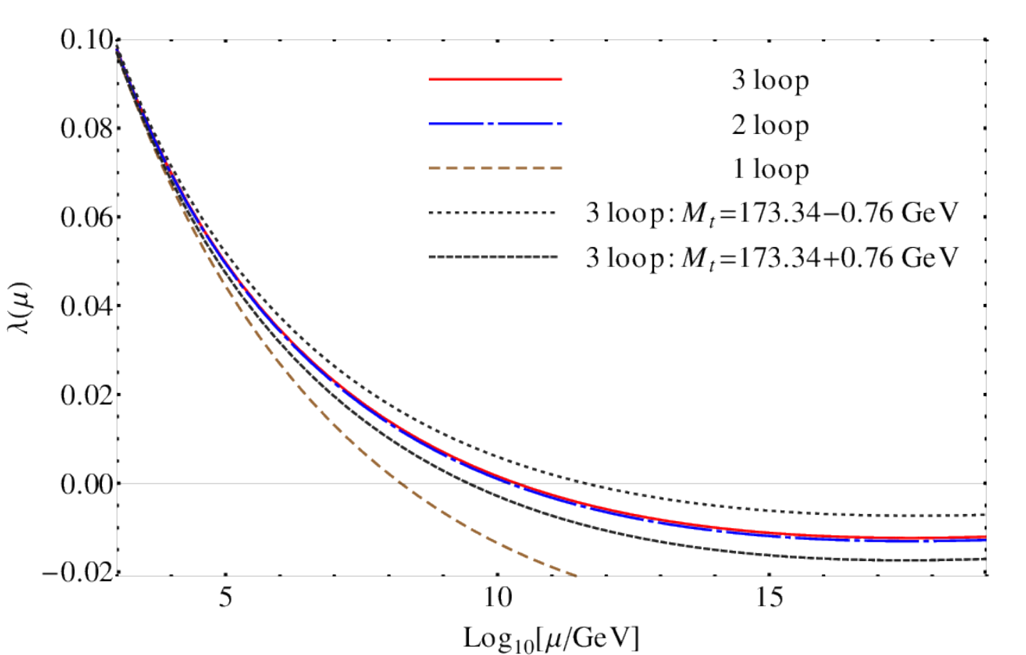
As a further example we show in Fig. 10 the running of the quartic coupling up to the Planck scale with initial conditions taken for $\mu=M_{t}$. One observes quite significant effects when going from one- to two-loop accuracy. The three-loop corrections only lead to a small shift indicating a stabilization of the perturbative expansion. Notably, the theory uncertainty due to the running is now negligible as compared to the parametric one which is dominated by the top quark mass. In Fig. 10 the corresponding effect is shown as dotted lines. From Fig. 10 one deduces that $\lambda$ becomes negative for $\ln(\mu/\mbox{GeV})\;\hbox to0.0pt{\lower 3.5pt\hbox{$\mathchar 0\sim$}\hss}\raise 1.0pt\hbox{$>$}\;10.36$ [176]. Further details can be found in Subsection 4.10.

Before we report on the diagrammatic calculation of the three-loop gauge beta function in the supersymmetric QCD, few comments on the used regularisation scheme are in order.

Whereas Dimensional Regularization in combination with the $\overline{\rm MS}$ scheme is the canonical choice for higher order calculations within QCD, it is less appropiate for supersymmetric theories since it explicitely breaks supersymmetry. This can easily be understood by counting degrees of freedom of fermionic and spin-1 fields. Whereas the former has four degrees of freedom the latter has $d$ degrees, where $d$ is the space-time dimension and $d\not=4$. Thus a modification of the theory is necessary to render the two numbers equal. A convenient choice has been introduced in Ref. [177], so-called Dimensional Reduction. The essential difference between Dimensional Reduction and Dimensional Regularization is that the continuation from $4$ to $d$ dimensions is made by compactification or dimensional reduction. In this scheme, the momentum (or space-time) integrals are $d$-dimensional in the usual way, whereas the number of field components remains unchanged equal to four, and consequently supersymmetry is undisturbed (see also Refs. [178, 179].) In practice it is convenient to implement Dimensional Reduction by introducing a new particle, the so-called $\varepsilon$ scalar, that account for the additional $4-d$ components of the gauge boson fields. In this way, the well-established rules for computing momentum intregrals in Dimensional Regularization can also be applied to calculations performed in Dimensional Reduction.

An explicit calculation of the three-loop beta function for supersymmetric QCD has been performed in Ref. [175] confirming results which have previously been available in the literature [180, 146]. The main purpose of Ref. [175] was to perform a consistency check of Dimensional Reduction as regularisation scheme for supersymmetric theories at three-loop order. For this goal, several renormalization constants in supersymmetric QCD has been computed to three-loop accuracy. It has been shown that the same beta function is obtained from all three-particle vertices involving gluons, gluinos and $\varepsilon$-scalars. The results of Ref. [175] explicitly demonstrates the consistency of Dimensional Reduction with supersymmetry and gauge invariance, an important pre-requisite for (high-order) precision calculations in supersymmetric theories, like the three-loop corrections to the Higgs boson mass, cf. Section. 2.

As a by-product of the calculation in [175], the predicted relation between the gauge beta function and the gluino mass anomalous dimension was verified to three-loop order. In addition, the three-loop results for the quark mass anomalous dimension [181] were confirmed.

The use of Dimensional Reduction (in contrast to Dimensional Regularization) is one of the technical challenges of the calculation. A further difficulty, which is discussed in detail in Ref. [175], is the treatment of $\gamma_{5}$ which only plays a sub-leading role in the gauge coupling beta functions of the SM. Another technical complication is connected to the Majorana nature of the gluino which is not treated consistently in QGRAF [161] and thus a program, majoranas.pl, has been developed which implements the prescription of Ref. [182] and adjusts the output of QGRAF.

Let us for completeness present the result for the supersymmetric beta function up to three-loop order. Defining

we obtain for the first three coefficients

where $C_{F}=(n_{c}^{2}-1)/(2n_{c})$, $C_{A}=n_{c}$ are the quadratic Casimir invariants for SU($n_{c}$), and $2T_{f}=n_{f}$ is the number of quark flavors (which is equal to the number of squark flavors in supersymmetric QCD).

The anomalous dimensions considered in the previous subsections depend on the active degrees of freedom of the theory. In QCD, which for the following general discussion shall be used as a sample theory, this dependence is simply due to $n_{f}$, the number of quarks contributing to the running. In general, $n_{f}$ changes when flavour thresholds are crossed while increasing or lowering the energy scale. Note that it is not sufficient to simply raise or lower $n_{f}$ in the coefficients of the anomalous dimensions and continue the running of the corresponding parameters using the new beta function, but a careful construction of the low-energy effective theory is necessary. In the case of QCD this construction is straightforward since the effective theory with $n_{f}-1$ active quark flavours has the same structure, i.e., contains the same operators as the full theory. The fields, masses and couplings in the two theories are related by so-called decoupling constants. A detailed discussion and the explicit construction of the effective theory can be found in Refs. [41, 42]. In these references formulae for the decoupling constants are provided which allow to compute the $n$-loop decoupling constants from light-particle Green’s functions with vanishing external momenta. The formalism resembles the renormalization procedure in the $\overline{\rm MS}$ scheme. However, in contrast to the renormalization constants, the decoupling constants also contain finite (and also higher order $\epsilon$) terms.

We want to remark that the necessity of introducing decoupling constants originates from the use of a mass-independent (here $\overline{\rm MS}$) renormalization scheme. As a consequence the strong coupling constant $\alpha_{s}$ is not a physical quantity in the sense that it is not defined via a Green’s function which (at least in principle) can be measured. Furthermore, $\alpha_{s}(\mu)$ is not a continuous function of $\mu$ but has finite steps at the energy scale where the heavy quark is integrated out. In Refs. [183, 184] a physical definition of the strong coupling has been introduced in the so-called momentum subtraction (MOM) scheme and it has been shown that running in this scheme, where the decoupling of heavy particles is automatic, is equivalent to the running and decoupling procedure in the $\overline{\rm MS}$. Let us in the following briefly comment on the comparison of the MOM and $\overline{\rm MS}$ couplings before we continue our considerations in the $\overline{\rm MS}$ scheme.

In Fig. 11 we show that the two schemes are equivalent by plotting the inverse strong coupling as a function of $\mu$ both for the $\overline{\rm MS}$, MOM and $\overline{\rm MOM}$⁸⁸ 8 The $\overline{\rm MOM}$ scheme is a version of the MOM scheme which leads to numerical values for $\alpha_{s}$ close to the ones in the $\overline{\rm MS}$ scheme. schemes, where in all cases the three-loop approximation is used for the running and the conversion between the schemes. We choose $\alpha_{s}^{(5)}(M_{Z})$ as the input quantity and convert at this scale to the other two schemes. The evolution of the $\overline{\rm MS}$ coupling to lower $\mu$ values is shown by the upper solid lines with a step at the value $\mu=2M_{b}$ since at that scale the bottom quark is decoupled. Numerically very close is the dashed curve representing the $\overline{\rm MOM}$ scheme result. The lower solid line represents the result in the MOM scheme. Both for the MOM and $\overline{\rm MOM}$ results, the conversion is performed for $\mu=M_{Z}$, and the running to other values of $\mu$ is achieved using the corresponding $\beta$ function. The dotted lines on top of the MOM and $\overline{\rm MOM}$ curves represent the results where the transformation from the $\overline{\rm MS}$ values is performed just at the considered value of $\mu$. This shows that the $\overline{\rm MS}$ scheme including the described decoupling procedure is equivalent to a physical scheme with a physical definition of $\alpha_{s}$.

Let us now return to QCD with $\alpha_{s}$ defined in the $\overline{\rm MS}$ scheme. The phenomenologically most important decoupling constants are the ones of $\alpha_{s}$, $\zeta_{\alpha_{s}}$, and the light quark masses, $\zeta_{m_{q}}$. Two-loop corrections to $\zeta_{\alpha_{s}}$ have been computed for the first time in Refs. [185, 186], however, relatively complicated integrals had to be solved. For example, in Ref. [186] a three-loop calculation for the $Z$ boson decay rate has been performed. In Ref. [41] the two-loop result has been checked and the three-loop results for $\zeta_{\alpha_{s}}$ and $\zeta_{m_{q}}$ has been added. The latter required the computation of three-loop one-scale vacuum integrals. The four-loop corrections to the decoupling constants have been obtained by two independent calculations performed in Refs. [44, 45].

The loop-order used for the running and the one used for the decoupling are related. In fact, $n$-loop running requires $(n-1)$-loop decoupling relations. This can be seen by considering a physical quantity $R$ for which the perturbative expansion is know up to order $\alpha_{s}^{n}$. Of course, in such a situation one would apply $n$-loop corrections to the beta function. However, using $n$-loop decoupling relations would affect the $\alpha_{s}^{(n+1)}$ term of $R$ which is beyond the considered loop-order.

Let us in the following demonstrate the effect of higher order corrections to the running and decoupling by considering the relation between $\alpha_{s}^{(3)}(M_{\tau})$ and $\alpha_{s}^{(5)}(M_{Z})$ (see also Refs. [187, 41, 44, 45] where the charm and bottom flavour threshold is crossed at the scales $\mu_{c}$ and $\mu_{b}$, respectively. Note that these scales are not determined by theory. On general grounds one expects that the result for $\alpha_{s}^{(5)}(M_{Z})$ gets more and more insensitive on the precise choice of the decoupling scales when including higher order corrections. The procedure to compute $\alpha_{s}^{(5)}(M_{Z})$ from $\alpha_{s}^{(3)}(M_{\tau})$ is as follows. In a first step we calculate $\alpha_{s}^{(3)}(\mu_{c})$ by integrating the beta function to $n$-loop order with the initial condition $\alpha_{s}^{(3)}(M_{\tau})=0.332$. Afterwards $\alpha_{s}^{(4)}(\mu_{c})$ is obtained from $\alpha_{s}^{(3)}(\mu_{c})=\alpha_{s}^{(4)}(\mu_{c})\zeta_{\alpha_{s}}$ using the $(n-1)$-loop approximation for $\zeta_{\alpha_{s}}$. Next $n$-loop running is used to obtain $\alpha_{s}^{(4)}(\mu_{b})$ and the decoupling procedure is applied in analogy to the charm threshold to arrive at $\alpha_{s}^{(5)}(\mu_{b})$. Finally, we compute $\alpha_{s}^{(5)}(M_{Z})$ using again the $n$-loop beta function. For the on-shell charm and bottom quark masses we use $M_{c}=1.65$ GeV and $M_{b}=4.75$ GeV, respectively. These values are obtained by using three-loop relations between the $\overline{\rm MS}$ and on-shell quark masses [28, 29, 30].

In Fig. 12 the result for $\alpha_{s}^{(5)}(M_{Z})$ for fixed $\mu_{c}=3$ GeV as a function of $\mu_{b}$ is displayed for the one- to five-loop analysis. For illustration, $\mu_{b}$ is varied rather extremely, by about two orders of magnitude. While the leading-order result (upper right dotted line) exhibits a strong logarithmic behaviour, the analysis is gradually getting more stable as we go to higher orders. The five-loop curve is almost flat for $\mu_{b}\geq 1$ GeV (note the scale on the $y$ axis) and demonstrates an even more stable behaviour than the four-loop analysis of Ref. [41]. It should be noted that around $\mu_{b}\approx 1$ GeV both the three-, four- and five-loop curves show a strong variation which can be interpreted as a sign for the breakdown of perturbation theory. Besides the $\mu_{b}$ dependence of $\alpha_{s}^{(5)}(M_{Z})$, also its absolute normalization is significantly affected by the higher orders. At the central matching scale $\mu_{b}=M_{b}$, we encounter a rapid convergence behaviour.

Since the five-loop coefficient of the QCD beta function is not yet known we choose the ($n_{f}$-independent) values $\beta_{4}^{(n_{f})}=0$ (solid line) and $\beta_{4}^{(n_{f})}=150$ (dashed line parallel to the solid one)⁹⁹ 9 The normalization corresponding to $\{\beta_{0},\beta_{1},\beta_{2},\beta_{3}\}\approx\{1.92,2.42,2.83,18.85\}$ for $n_{f}=5$.. Larger values would bring the five-loop curves even closer to the four-loop one.

From Fig. 12 it is possible to estimate a theory uncertainty on $\alpha_{s}^{(5)}(M_{Z})$ as obtained from $\alpha_{s}^{(3)}(M_{\tau})$ due to missing higher order corrections. If we restrict ourselves to a range of $\mu_{b}$ between 2 GeV and 10 GeV and take the difference between the three- and four-loop curve as an estimate for the uncertainty we obtain $\delta\alpha_{s}^{(5)}(M_{Z})\approx 0.0002$. The difference between the four- and (dashed) five-loop curve would lead to $\delta\alpha_{s}^{(5)}(M_{Z})\approx 0.0003$. The variation of $\alpha_{s}^{(5)}(M_{Z})$ due to the variation of $\mu_{b}$ leads to an additional uncertainty of $\delta\alpha_{s}^{(5)}(M_{Z})\approx 0.0002$. A similar uncertainty is obtained from the variation of $\mu_{c}$ between 2 GeV and 5 GeV. (This can easily be checked with the program RunDec [188].) Thus a total uncertainty of $\pm 0.0004$ (obtained by adding the three uncertainties in quadrature) should be assigned to $\alpha_{s}^{(5)}(M_{Z})$. The uncertainties induced by the errors in the quark masses are much smaller.

Note that it is straightforward to reproduce Fig. 12 using the program RunDec [188] which is written in Mathematica or CRunDec [189] written in C++.

The formalism which has been described above allows the decoupling of one heavy quark at a time. This procedure is certainly justified for the top quark being more than factor 30 heavier than the bottom quark. On the other hand, the ratio between the bottom and charm quark mass is only approximately a factor three. For this reason the simultaneous decoupling of the charm and bottom has been studied in Ref. [190] and a decoupling constant relating the strong coupling defined with three active flavours to the one in the five-flavour theory has been derived. These results can be used in order to study the effect of power-suppressed terms in $M_{c}/M_{b}$ which are neglected in the conventional approach [41]. Various analyses are performed which indicate that the mass corrections present in the one-step approach are small as compared to $\log(\mu^{2}/M_{c,b}^{2})$ which are resummed using the conventional two-step procedure, and, thus, even for the charm and bottom quark case two-step decoupling is preferable.

As in QCD also in its supersymmetric extension, it is convenient to use a mass-independent renormalization scheme. Thus, by construction, the beta function governing the running of $\alpha_{s}$ is independent of the particle masses. It only depends on the particle content of the underlying theory, i.e., the number of active quarks, squarks and gluinos.

In the MSSM, the one-loop decoupling relation for $\alpha_{s}$ has been computed in Refs. [191, 109] and the two-loop relation is known from Refs. [192, 193, 194] (see also Ref. [195]). Due to many different mass scales exact results cannot be obtained at three loops. Thus, in Ref. [121] three different hierarchies among the supersymmetric particle masses have been assumed to compute the decoupling relation.

Let us in the following demonstrate the numerical effect of higher order corrections to the decoupling constants by repeating the considerations of Subsection 4.5. However, instead of considering the strong coupling with three and five active flavours we study the relation between $\alpha_{s}^{\rm(SQCD)}(M_{\rm GUT})$ (defined in the $\overline{\rm DR}$ scheme) with $M_{\rm GUT}=2\cdot 10^{16}$ GeV and $\alpha_{s}^{(5)}(M_{Z})$ (in the $\overline{\rm MS}$ scheme) as a function of the decoupling scale $\mu_{\rm dec}$. At this scale all supersymmetric particles are integrated out and the transition from the MSSM to the SM is made. We proceed as follows: In a first step we run in the SM from $\mu=M_{Z}$ to $\mu=\mu_{\rm dec}$ where the decoupling of the top quark and the supersymmetric particles is performed simultaneously and $\alpha_{s}^{(5)}(\mu_{\rm dec})$ is transformed to $\alpha_{s}^{(\rm SQCD)}(\mu_{\rm dec})$. The use of the SUSY QCD $\beta$ function finally leads to $\alpha_{s}^{\rm(SQCD)}(M_{\rm GUT})$. The thick lines in Fig. 13 correspond to this procedure where dotted, dash-dotted, dashed and solid lines correspond to one-, two-, three- and four-loop running and the use of decoupling constants to one order less. For a complete list of input parameters we refer to Ref. [121].

As expected, the inclusion of higher order corrections reduces dramatically the dependence on $\mu_{\rm dec}$ leading to an almost flat behaviour at four loops, even though the decoupling scale is varied over more than two orders of magnitude. The band around the four-loop curve reflects the uncertainty of the strong coupling constant which has been chosen as $\alpha_{s}^{(5)}(M_{Z})=0.1184\pm 0.0007$. It is interesting to note that $\mu_{\rm dec}=M_{Z}$ is in general a less favourable choice unless three- or four-loop running is used. On the contrary, for $\mu_{\rm dec}\approx 1$ TeV, which approximatley corresponds to the masses of the supersymmetric particles, higher order corrections are quite small.

Alternatively, in order to obtain the thin lines we integrate out the top quark in a separate step at the scale $\mu=M_{t}$ ($M_{t}$ is the on-shell top quark mass) and transform afterwards $\alpha_{s}^{(6)}(M_{t})$ to $\alpha_{s}^{(\rm SQCD)}(M_{\rm GUT})$ in analogy to the previous description. The three- and four-loop curves show in this variant an even flatter behaviour.

Another type of threshold corrections that have to be considered in the context of GUTs are those generated by the super-heavy particles present in such models. In particular, the gauge coupling unification (one of the most important predictions of a GUT) is very sensitive to these corrections. This property enables us to constrain the models, once the low energy values of the gauge couplings and their evolution are known precisely. In the following, we restrict our discussion to the effects of the threshold corrections at the super-heavy scale on the energy evolution of the SM gauge couplings.

The new features of the GUT threshold corrections as compared with those discussed in the previous subsections are related to the spontaneous breaking of the gauge symmetry. Explicitly, they take into account the effects of the spontaneous breaking of the GUT gauge group to the SM gauge group. In consequence, the three SM gauge couplings are affected differently by these corrections, so that after passing the super-heavy threshold they become equal and evolve as a unique coupling towards the Planck scale. Furthermore, the calculation of the associated decoupling constants is much more involved and very model dependent. Another subtle point concerns the choice of gauge within the full theory so that the gauge invariance of the effective theory, obtained by integrating out the heavy degrees of freedom, is also maintained [196].

Currently, the super-heavy threshold corrections to the gauge couplings are known at the one-loop level for a general model [191, 196]. However, at the two-loop level there are only the attempts of Refs. [197, 198] towards a general derivation. Precisely, this computation covers only theories without super-heavy fermions and with a rather simplified structure for the GUT breaking scalars. Also, trilinear interactions in the scalar potential are not considered. Thus, their applicability to specific models is rather restricted.

For exemplification, we show in Fig. 14 sample Feynman diagrams contributing at the two-loop level to the decoupling constant of the gauge couplings. As usual, to compute the decoupling constants one considers Green’s functions involving only light external particles and at least one heavy field within the loops. In Fig. 14 the contributions to the self-energies of the light gauge bosons and their associated ghosts, and to the gauge boson-ghost three-point function are shown.

A numerical analysis of the effect of the two-loop GUT threshold corrections on gauge coupling unification was performed in Ref. [197]. It turned out that, for models containing large representations, the effects of the two-loop GUT threshold corrections exceed by almost an order of magnitude those induced by the current experimental uncertainties of the gauge coupling constants. In consequence, the GUT threshold corrections necessarily have to be taken into account in any phenomenological study concerning the gauge coupling unification. An impression of their numerical effects in the minimal SUSY SU(5) model can be seen in Fig. 16(b) (however, only at the one-loop level).

There is a close connection between the decoupling constants and the effective coupling of a Higgs boson to gluons and light quarks which at first sight is quite surprising. It is established by the so-called low-energy theorem (LET) which relates the decoupling constants to the Wilson coefficients in the effective Lagrangian

where the first part has already been shown in Eq. (8). The term proportional to $C_{2}$ has been specified to the bottom quarks; similar contributions also exist for the other light quarks. In Ref. [41] the following LETs have been derived

where we refer to [41] for a proper definition of the decoupling constants (with $\zeta_{\alpha_{s}}=(\zeta_{g})^{2}$).

At lowest order the LETs given in Eq. (27) can easily be motivated. Consider, e.g., $C_{1}$ which can be computed from the one-loop top quark triangle with two gluons and a zero-momentum Higgs boson as external particle. On the other hand, only the one-loop heavy-top diagram of the gluon propagator contributes to $\zeta_{\alpha_{s}}$. Zero-momentum top quark-Higgs boson coupling are obviously generated by taking derivatives with respect to the top quark mass which leads to the first line in Eq. (27) expanded to one-loop order. At higher order this simple picture does not work any more due to the fact that also other Green’s functions enter $\zeta_{\alpha_{s}}$, e.g., the ghost two-point function.

It is interesting to note that Eq. (27) only contains logarithmic derivatives. Thus, it is sufficient to know the $\ln(m_{t}^{2})$ terms of $\zeta_{\alpha_{s}}$ and $\zeta_{m_{q}}$ in order to obtain $C_{1}$ and $C_{2}$ at the respective loop order. Since $m_{t}$ is the only dimensionful physical scale it actually occurs in the combination $\ln(\mu^{2}/m_{t}^{2})$ and thus the logarithms at order $\alpha_{s}^{(n+1)}$ can be reconstructed from the order $\alpha_{s}^{n}$ with the help of renormalization group functions. In Refs. [44, 45] this has been exploited to obtain the five-loop result for $C_{1}$ from the four-loop result of $\zeta_{\alpha_{s}}$.¹⁰¹⁰ 10 Note that the fermionic contribution of the five-loop beta function, which is not yet known, enters the five-loop term of $C_{1}$ as a free parameter. In beyond-SM theories this trick cannot be applied due to the presence of more than one particle mass.

For earlier work on LETs we want to refer to Refs. [199, 200] and for the application of LETs in supersymmetric theories we want to mention the works [110, 201, 121]. In Ref. [190] it has been applied to QCD involving more than one heavy quark.

The quantum numbers of the SM fermions together with the apparent convergence of the strong and electroweak couplings at energies below the Planck scale point towards a unified description of the SM interactions. Furthermore, one of the fundamental predictions of a GUT is the existence of baryon and lepton number violating interactions which can manifest themselves at low energy via matter instability (for a review see for example Ref. [202]). Though the decay of the proton has not been observed so far, the lower bound on the proton lifetime together with the low-energy values of the SM gauge couplings and the SM fermion masses and mixing provide us severe constraints on the class of viable GUT models.

Gauge coupling unification is highly sensitive to the mass spectrum. This property allows us to probe the unification assumption through precision measurements of low-energy parameters like the gauge couplings at the electroweak scale or the mass spectrum and precision calculations. Through such analyses, we can make predictions for some of the mass parameters of the models that have to be compared with the constraints derived from the non-observation of the proton decay. In addition, GUTs might predict interesting signatures at the LHC (see, e.g., Ref. [203] for a recent search for heavy fermionic triplets and Ref. [204] for searches for scalar leptoquarks). These additional constraints from the LHC can, in some cases, be sufficient to even rule out models [205, 206, 207, 208, 209].

In the following, we restrict our discussion to GUTs based on the SU(5) gauge group. Although phenomenologically there are other theories which are better motivated, SU(5) GUTs are most predictive. For example, one of the few absolute certainties about grand unification today is that the original SU(5) model of Georgi and Glashow (GG) [210] is ruled out. In particular, the failure of the minimal model can be attributed partially to the lack of gauge coupling unification [211, 212, 213].

Let us briefly recall the reason why gauge coupling unification fails within the minimal GG model.¹¹¹¹ 11 For the definition of $\alpha_{1}$, $\alpha_{2}$ and $\alpha_{3}$ see Eq. (16). While $\alpha_{2}$ and $\alpha_{3}$ meet around $10^{16}$ GeV, $\alpha_{1}$ and $\alpha_{2}$ intersect already at about $10^{13}$ GeV, at odds with the bounds enforced by the nonobservation of the proton decay. More precisely, model independent upper bounds on the proton lifetime [214] together with the latest experimental data from the Super-Kamiokande observatory [215] imply a conservative lower bound on the unification scale $M_{G}$ of about $10^{15.5}\ \rm{GeV}$. Hence, the key ingredients for a viable unification pattern are additional particles charged under the ${\rm SU(2)}_{L}$ group that delay the meeting of $\alpha_{1}$ and $\alpha_{2}$. This is, essentially, the philosophy behind two recent proposals where an extra scalar representation $15_{H}$ [216, 217], or alternatively, a fermionic representation $24_{F}$ [218, 205] are added to the field content of the model. In both cases, the extra degrees of freedom have the correct quantum numbers to restore unification by properly modifying the running of the gauge couplings.

In particular, the study performed in Ref. [209] proved that a three-loop analysis of the gauge coupling unification is required within the SU(5)+$24_{F}$ model. As can be read from the Fig. 15, the two-loop corrections to the mass of the electroweak triplets $m_{3}$ for a fixed unification scale $M_{G}$ is of the same order of magnitude as the one-loop contributions and amount to several TeV. The three-loop corrections are rather small (hundreds of GeV) and lie within the uncertainty band of the two-loop results. Thus, the three-loop order analysis is required in order to reduce the theoretical uncertainties at the level of parametric uncertainties induced by the low-energy measurements of the electroweak gauge couplings. Moreover, the achieved theoretical accuracy together with experimental data in the reach of the LHC and the Super-Kamiokande observatory will provide us with sufficient information to even disprove the model.

Another example of a predictive GUT model is the minimal SUSY SU(5) [219, 220]. It has the important feature that one can derive unambiguous correlations among its parameters and even rule out the model once sufficiently precise experimental data become available. Immediately after the formulation of the minimal SUSY SU(5) it has been noticed that within SUSY GUTs new dimension-five operators cause a rapid proton decay [221, 222]. This aspect was intensively studied over the last thirty years with the extreme conclusions of Refs. [223, 224] that the minimal SUSY SU(5) model is ruled out by the combined constraints from proton decay and gauge coupling unification. However, careful analyses have shown that taking into account fermion mixing [225] or higher dimensional operators induced at the Planck scale [226, 227], one can substantially weaken the constraints and the minimal model remains a valid theory. Also the high-precision analysis of Ref. [228] confirmed that the minimal SUSY SU(5) model cannot be excluded by the current experimental data. In particular, one observes an increase of the super-heavy Higgs triplet mass by about an order of magnitude when three-loop effects are considered. These results attenuate substantially the tension between the theoretical predictions and the constraints derived from the experimental data.

Beyond the minimal version of the SUSY SU(5) model, the interplay between the theoretical predictions and the experimental data is not completely determined. For example, the most popular extension of the minimal SUSY SU(5) model, the Missing Doublet Model [229, 230], designed to avoid unnatural doublet-triplet splitting, cannot be excluded using only the currently available theoretical and experimental data. The model contains additional free parameters as compared to the minimal model and, consequently, is affected by large theoretical uncertainties, so that no firm conclusion can be drawn.

For illustration, we briefly discuss the analysis of the gauge coupling unification in the SUSY SU(5) model at three-loop level. Crucial input parameters for this analysis are the precise values of the gauge couplings at the electroweak scale. For their determination from the experimentally measured observables, one has to take into consideration threshold corrections at the Z-boson mass and at the top quark mass (for a detailed description see Ref. [228]). Furthermore, one applies the “running and decoupling” approach described in the previous sections. The dependence on the heavy particle masses becomes explicit through the decoupling constants. The constraint of gauge coupling unification translates into restrictions (usually expressed as correlations) on the mass spectrum.

In Fig. 16 the evolution of the SM gauge couplings from the electroweak up to the Planck scale is shown in the minimal SUSY SU(5) model. The specific threshold corrections for this model are those due to supersymmetric particles at the TeV scale and those due to super-heavy particles at around $10^{16}$ GeV. The associated decoupling scales have been chosen at $\mu_{\rm SUSY}=1000$ GeV and $\mu_{\rm GUT}=10^{16}$ GeV. One can clearly see the discontinuities at the matching scales and the change of the slopes when passing them. The (blue) band around the strong coupling corresponds to the present experimental uncertainty. In panel (b) the region around $\mu=10^{16}$ GeV is enlarged which allows for a closer look at the unification region. Here, the decoupling of the super-heavy particles is performed at two different values of $\mu_{\rm GUT}$. One observes quite different threshold corrections leading to a nice agreement of the (common) gauge coupling above $10^{16}$ GeV. On the one hand, the plot proves that the GUT threshold corrections are essential for a successful unification. On the other hand, the dependence on $\mu_{\rm GUT}$ is interpreted as a measure of theoretical uncertainties because this parameter is not fixed by the theory. Thus, the three-loop analysis is sufficient to cope with the current experimental precision.

To summarise, threshold corrections at the GUT scale are indispensable ingredients for precision analyses of gauge coupling unification. In particular, they have the virtue to provide us with the necessary information about the specific model dependence. In this way, we are able to perform consistency tests of various GUTs and, in some cases, even to refute models.

With the discovery of a Higgs boson at the LHC, the question of the SM vacuum stability received a renewed attention. This is because the mass of the Higgs boson in the SM is an important indicator for the presence of new physics at high energy scales. It is well known that, if the Higg boson mass satisfies the condition $M^{\rm meta}<M_{h}<M^{\rm Landau}$ then the SM is a consistent theory from the electroweak scale up to the Planck scale. The upper limit originates from the requirement that the Higgs self-coupling remains in the perturbative regime up to the Planck scale. Explicitly, the occurrence of the Landau pole is avoided. The estimated value for $M^{\rm Landau}$ is around $175$ GeV [231], which is excluded by the direct searches at the LHC and the Tevatron. The lower limit is derived from instability constraints. The existence of a Higgs boson with a mass smaller than $M^{\rm meta}$ would imply that new physics below the Planck scale is required to stabilize the SM vacuum. The numerical value for $M^{\rm meta}$ was estimated to $111$ GeV [232]. In consequence, for a Higgs boson with mass $M_{h}\approx 125$ GeV one distinguishes two situations: either $M_{h}>M^{\rm stability}$ and the electroweak vacuum is absolutely stable, or $M^{\rm meta}<M_{h}<M^{\rm stability}$, which corresponds to a metastable vaccum with a life-time exceeding that of the Universe.

The precise determination of $M^{\rm stability}$ was the subject of numerous recent analyses [233, 26, 234, 235]. The absolute stability bound on the Higgs mass $M^{\rm stability}$ is defined as the value for which the effective potential at the electroweak minimum, $\phi_{\rm{ew}}$, and at a second minimum at large field values, $\tilde{\phi}>\phi_{\rm{ew}}$, are the same. The equations to be solved read

Although the effective potential as well as the positions of its extrema are both gauge dependent, the solution for $M^{\rm stability}$ is gauge independent as shown in Ref. [236].

The most advanced recent works use for the calculation of $M^{\rm stability}$ the two-loop SM effective potential [141, 237] and the three-loop RGEs for the SM couplings [147, 148, 149, 152, 153, 155, 156], necessary to resum the large logarithms that occur in the effective potential $V$ for large field values. In addition, two-loop corrections to the relations between the $\overline{\text{MS}}$ parameters and the physical observables have been considered in Refs. [233, 26, 235]. The phenomenological implications of the new determination of $M^{\rm stability}$ are summarised in the phase diagram shown in Fig. 17. The regions of stability, metastability and instability of the SM vacuum are shown for Higgs boson ($M_{h}$) and top quark ($M_{t}$) masses in the range corresponding to the measured values. Also shown are contour lines indicating the instability scale $\Lambda_{\rm SM}$, defined as the scale where new physics is required to stabilize the SM effective potential. It appears that the measured values for $M_{h}$ and $M_{t}$ are rather special, in the sense that, the SM vacuum lies at the border between stability and metastability. One also concludes that a metastable electroweak vacuum can comply with the data and new physics below the Planck scale is not necessarily implied.

Note that the interpretation of the SM instability scale as the scale $\Lambda$, where

is problematic. The effective potential is gauge dependent, and it renders $\Lambda$ as solution of the inequality (29) gauge dependent as well. The numerical effects due to gauge dependence are rather large as has been explicitly shown in Refs. [236, 238, 239]. The instability scale can vary by few orders of magnitude in $R_{\xi}$-like gauges, depending on the choice of the gauge fixing parameters. This behaviour is illustrated in Fig. 18 taken from Ref. [236]. Here, the dependence of the SM instability scale [defined as in inequality (29)] on a common gauge fixing parameter in the electroweak sector is displayed for the special choice of a Fermi gauge (see Ref. [236] for precise definition). As can be read from the figure, the resummation obtained through the use of running gauge fixing parameters is essential to reduce the variation of the instability scale. However, even the RGE improved prediction for $\Lambda_{\rm SM}$ varies by an order of magnitude for gauge fixing parameters in the perturbative regime. Let us at this point stress that significant variations of the instability scale are also observed when changing the form of the gauge fixing term in the Lagrange density.

To conclude, a metastable electroweak vacuum can comply with the present experimental data, and new physics below the Planck scale is not necessarily required. Furthermore, the physical threshold for new physics can be determined only after specifying an ultraviolet completion of the SM. Its determination from the stability requirement of the SM potential is theoretically inconsistent due to the gauge dependence as discussed above.

References

- [1] G. Aad et al. [ATLAS Collaboration], Phys. Rev. D 90 (2014) 052004 [arXiv:1406.3827 [hep-ex]].
- [2] V. Khachatryan et al. [CMS Collaboration], arXiv:1412.8662 [hep-ex].
- [3] J. L. Feng, P. Kant, S. Profumo and D. Sanford, Phys. Rev. Lett. 111 (2013) 131802 [arXiv:1306.2318 [hep-ph]]. [175]
- [4] T. Hahn, S. Heinemeyer, W. Hollik, H. Rzehak and G. Weiglein, Phys. Rev. Lett. 112 (2014) 141801 [arXiv:1312.4937 [hep-ph]].
- [5] P. Draper, G. Lee and C. E. M. Wagner, Phys. Rev. D 89 (2014) 055023 [arXiv:1312.5743 [hep-ph]].
- [6] J. R. Ellis, G. Ridolfi and F. Zwirner, Phys. Lett. B 257 (1991) 83; Phys. Lett. B 262 (1991) 477.
- [7] Y. Okada, M. Yamaguchi and T. Yanagida, Prog. Theor. Phys. 85 (1991) 1.
- [8] H. E. Haber and R. Hempfling, Phys. Rev. Lett. 66 (1991) 1815.
- [9] P. H. Chankowski, S. Pokorski and J. Rosiek, Phys. Lett. B 274 (1992) 191.
- [10] A. Brignole, Phys. Lett. B 281, 284 (1992).
- [11] A. Dabelstein, Z. Phys. C 67 (1995) 495 [hep-ph/9409375].
- [12] S. Heinemeyer, Int. J. Mod. Phys. A 21 (2006) 2659 [hep-ph/0407244].
- [13] B. C. Allanach, A. Djouadi, J. L. Kneur, W. Porod and P. Slavich, JHEP 0409 (2004) 044 [arXiv:hep-ph/0406166].
- [14] S. Borowka, T. Hahn, S. Heinemeyer, G. Heinrich and W. Hollik, Eur. Phys. J. C 74 (2014) 2994 [arXiv:1404.7074 [hep-ph]].
- [15] G. Degrassi, S. Di Vita and P. Slavich, arXiv:1410.3432 [hep-ph].
- [16] M. Frank, T. Hahn, S. Heinemeyer, W. Hollik, H. Rzehak and G. Weiglein, JHEP 0702 (2007) 047 [hep-ph/0611326]; http://www.feynhiggs.de/.
- [17] S. Heinemeyer, W. Hollik, H. Rzehak and G. Weiglein, Phys. Lett. B 652 (2007) 300 [arXiv:0705.0746 [hep-ph]].
- [18] M. S. Carena, J. R. Ellis, A. Pilaftsis and C. E. M. Wagner, Nucl. Phys. B 586 (2000) 92 [hep-ph/0003180].
- [19] S. P. Martin, Phys. Rev. D 67 (2003) 095012 [hep-ph/0211366].
- [20] R. V. Harlander, P. Kant, L. Mihaila and M. Steinhauser, Phys. Rev. Lett. 100 (2008) 191602 [Phys. Rev. Lett. 101 (2008) 039901] [arXiv:0803.0672 [hep-ph]].
- [21] P. Kant, R. V. Harlander, L. Mihaila and M. Steinhauser, JHEP 1008 (2010) 104 [arXiv:1005.5709 [hep-ph]].
- [22] L. Mihaila, Adv. High Energy Phys. 2013 (2013) 607807 [arXiv:1310.6178 [hep-ph]].
- [23] V. A. Smirnov, “Applied asymptotic expansions in momenta and masses,” Springer Tracts Mod. Phys. 177 (2002) 1.
- [24] M. Steinhauser, Comput. Phys. Commun. 134 (2001) 335 [arXiv:hep-ph/0009029].
- [25] S. P. Martin, Phys. Rev. D 75 (2007) 055005 [hep-ph/0701051].
- [26] G. Degrassi, S. Di Vita, J. Elias-Miro, J. R. Espinosa, G. F. Giudice, G. Isidori and A. Strumia, JHEP 1208 (2012) 098 [arXiv:1205.6497 [hep-ph]].
- [27] D. Kunz, L. Mihaila and N. Zerf, JHEP 1412 (2014) 136 [arXiv:1409.2297 [hep-ph]].
- [28] K. G. Chetyrkin and M. Steinhauser, Phys. Rev. Lett. 83 (1999) 4001, arXiv:hep-ph/9907509.
- [29] K. G. Chetyrkin and M. Steinhauser, Nucl. Phys. B 573 (2000) 617, arXiv:hep-ph/9911434.
- [30] K. Melnikov and T. v. Ritbergen, Phys. Lett. B 482 (2000) 99, arXiv:hep-ph/9912391.
- [31] S. Heinemeyer, W. Hollik and G. Weiglein, Comput. Phys. Commun. 124 (2000) 76 [hep-ph/9812320].
- [32] J. S. Lee, A. Pilaftsis, M. S. Carena, S. Y. Choi, M. Drees, J. R. Ellis and C. E. M. Wagner, Comput. Phys. Commun. 156 (2004) 283 [arXiv:hep-ph/0307377]. J. S. Lee, M. Carena, J. Ellis, A. Pilaftsis and C. E. M. Wagner, Comput. Phys. Commun. 180 (2009) 312 [arXiv:0712.2360 [hep-ph]].
- [33] P. Marquard and N. Zerf, Comput. Phys. Commun. 185 (2014) 1153 [arXiv:1309.1731 [hep-ph]].
- [34] P. Z. Skands, B. C. Allanach, H. Baer, C. Balazs, G. Belanger, F. Boudjema, A. Djouadi and R. Godbole et al., JHEP 0407 (2004) 036 [hep-ph/0311123].
- [35] B. C. Allanach, Comput. Phys. Commun. 143 (2002) 305 [arXiv:hep-ph/0104145].
- [36] W. Porod, Comput. Phys. Commun. 153 (2003) 275 [hep-ph/0301101].
- [37] A. Djouadi, J. -L. Kneur and G. Moultaka, Comput. Phys. Commun. 176 (2007) 426 [hep-ph/0211331].
- [38] S. Dittmaier, C. Mariotti, G. Passarino, R. Tanaka et al., [LHC Higgs Cross Section Working Group Collaboration], arXiv:1101.0593 [hep-ph].
- [39] S. Dittmaier, C. Mariotti, G. Passarino, R. Tanaka et al., [LHC Higgs Cross Section Working Group Collaboration], arXiv:1201.3084 [hep-ph].
- [40] S. Heinemeyer et al. [LHC Higgs Cross Section Working Group Collaboration], arXiv:1307.1347 [hep-ph].
- [41] K. G. Chetyrkin, B. A. Kniehl and M. Steinhauser, Nucl. Phys. B 510 (1998) 61, arXiv:hep-ph/9708255.
- [42] M. Steinhauser, Phys. Rept. 364 (2002) 247, arXiv:hep-ph/0201075.
- [43] M. Kramer, E. Laenen and M. Spira, Nucl. Phys. B 511 (1998) 523 [arXiv:hep-ph/9611272].
- [44] Y. Schröder and M. Steinhauser, JHEP 0601 (2006) 051, arXiv:hep-ph/0512058.
- [45] K. G. Chetyrkin, J. H. Kühn and C. Sturm, Nucl. Phys. B 744 (2006) 121, arXiv:hep-ph/0512060.
- [46] R. V. Harlander and K. J. Ozeren, JHEP 0911 (2009) 088 [arXiv:0909.3420 [hep-ph]].
- [47] A. Pak, M. Rogal and M. Steinhauser, JHEP 1002 (2010) 025 [arXiv:0911.4662 [hep-ph]].
- [48] R. V. Harlander, H. Mantler, S. Marzani and K. J. Ozeren, Eur. Phys. J. C 66 (2010) 359 [arXiv:0912.2104 [hep-ph]].
- [49] A. Pak, M. Rogal and M. Steinhauser, JHEP 1109 (2011) 088 [arXiv:1107.3391 [hep-ph]].
- [50] C. Anastasiou, S. Beerli and A. Daleo, Phys. Rev. Lett. 100 (2008) 241806 [arXiv:0803.3065 [hep-ph]].
- [51] F. Wilczek, Phys. Rev. Lett. 39 (1977) 1304.
- [52] J. R. Ellis, M. K. Gaillard, D. V. Nanopoulos and C. T. Sachrajda, Phys. Lett. B 83 (1979) 339.
- [53] H. M. Georgi, S. L. Glashow, M. E. Machacek and D. V. Nanopoulos, Phys. Rev. Lett. 40 (1978) 692.
- [54] T. G. Rizzo, Phys. Rev. D 22 (1980) 178 [Addendum-ibid. D 22 (1980) 1824].
- [55] S. Dawson, Nucl. Phys. B 359 (1991) 283.
- [56] M. Spira, A. Djouadi, D. Graudenz and P. M. Zerwas, Nucl. Phys. B 453 (1995) 17, arXiv:hep-ph/9504378.
- [57] R. Harlander and P. Kant, JHEP 0512 (2005) 015 [arXiv:hep-ph/0509189].
- [58] S. Actis, G. Passarino, C. Sturm and S. Uccirati, Phys. Lett. B 670 (2008) 12, arXiv:0809.1301 [hep-ph].
- [59] C. Anastasiou, R. Boughezal and F. Petriello, JHEP 0904 (2009) 003 [arXiv:0811.3458 [hep-ph]].
- [60] R. V. Harlander, Phys. Lett. B 492 (2000) 74, arXiv:hep-ph/0007289.
- [61] R. V. Harlander and W. B. Kilgore, Phys. Rev. Lett. 88 (2002) 201801, arXiv:hep-ph/0201206.
- [62] C. Anastasiou and K. Melnikov, Nucl. Phys. B 646 (2002) 220, arXiv:hep-ph/0207004.
- [63] V. Ravindran, J. Smith and W. L. van Neerven, Nucl. Phys. B 665 (2003) 325, arXiv:hep-ph/0302135.
- [64] R. V. Harlander and W. B. Kilgore, JHEP 0210 (2002) 017 [hep-ph/0208096].
- [65] C. Anastasiou and K. Melnikov, Phys. Rev. D 67 (2003) 037501 [hep-ph/0208115].
- [66] R. Harlander, Eur. Phys. J. C 33 (2004) S454 [arXiv:hep-ph/0311005].
- [67] S. Catani, D. de Florian, M. Grazzini and P. Nason, JHEP 0307 (2003) 028, arXiv:hep-ph/0306211.
- [68] V. Ahrens, T. Becher, M. Neubert and L. L. Yang, Phys. Lett. B 698 (2011) 271 [arXiv:1008.3162 [hep-ph]].
- [69] M. Bonvini, S. Forte, G. Ridolfi and L. Rottoli, arXiv:1409.0864 [hep-ph].
- [70] S. Moch and A. Vogt, Phys. Lett. B 631 (2005) 48 [hep-ph/0508265].
- [71] V. Ravindran, Nucl. Phys. B 752 (2006) 173 [arXiv:hep-ph/0603041].
- [72] S. Catani, L. Cieri, D. de Florian, G. Ferrera and M. Grazzini, Nucl. Phys. B 888 (2014) 75 [arXiv:1405.4827 [hep-ph]].
- [73] D. de Florian, J. Mazzitelli, S. Moch and A. Vogt, arXiv:1408.6277 [hep-ph].
- [74] V. Ahrens, T. Becher, M. Neubert and L. L. Yang, Eur. Phys. J. C 62 (2009) 333 [arXiv:0809.4283 [hep-ph]].
- [75] S. Marzani, R. D. Ball, V. Del Duca, S. Forte and A. Vicini, Nucl. Phys. B 800 (2008) 127 [arXiv:0801.2544 [hep-ph]].
- [76] R. V. Harlander and K. J. Ozeren, Phys. Lett. B 679 (2009) 467 [arXiv:0907.2997 [hep-ph]].
- [77] A. Pak, M. Rogal and M. Steinhauser, Phys. Lett. B 679 (2009) 473 [arXiv:0907.2998 [hep-ph]].
- [78] F. Caola and S. Marzani, Phys. Lett. B 698 (2011) 275 [arXiv:1101.3975 [hep-ph]].
- [79] M. Spira, arXiv:hep-ph/9510347.
- [80] P. A. Baikov, K. G. Chetyrkin, A. V. Smirnov, V. A. Smirnov and M. Steinhauser, Phys. Rev. Lett. 102 (2009) 212002 [arXiv:0902.3519 [hep-ph]].
- [81] T. Gehrmann, E. W. N. Glover, T. Huber, N. Ikizlerli and C. Studerus, JHEP 1006 (2010) 094 [arXiv:1004.3653 [hep-ph]].
- [82] R. N. Lee, A. V. Smirnov and V. A. Smirnov, JHEP 1004 (2010) 020 [arXiv:1001.2887 [hep-ph]].
- [83] S. Moch, J. A. M. Vermaseren and A. Vogt, Phys. Lett. B 625 (2005) 245 [hep-ph/0508055].
- [84] C. Anastasiou, S. Buehler, C. Duhr and F. Herzog, JHEP 1211 (2012) 062 [arXiv:1208.3130 [hep-ph]].
- [85] M. Höschele, J. Hoff, A. Pak, M. Steinhauser and T. Ueda, Phys. Lett. B 721 (2013) 244 [arXiv:1211.6559 [hep-ph]].
- [86] S. Buehler and A. Lazopoulos, JHEP 1310 (2013) 096 [arXiv:1306.2223 [hep-ph]].
- [87] M. Höschele, J. Hoff, A. Pak, M. Steinhauser and T. Ueda, Comput. Phys. Commun. 185 (2014) 528 [arXiv:1307.6925].
- [88] C. Duhr and T. Gehrmann, Phys. Lett. B 727 (2013) 452 [arXiv:1309.4393 [hep-ph]].
- [89] Y. Li and H. X. Zhu, JHEP 1311 (2013) 080 [arXiv:1309.4391 [hep-ph]].
- [90] F. Dulat and B. Mistlberger, arXiv:1411.3586 [hep-ph].
- [91] C. Duhr, T. Gehrmann and M. Jaquier, arXiv:1411.3587 [hep-ph].
- [92] C. Anastasiou, C. Duhr, F. Dulat, F. Herzog and B. Mistlberger, JHEP 1312 (2013) 088 [arXiv:1311.1425 [hep-ph]].
- [93] W. B. Kilgore, Phys. Rev. D 89 (2014) 073008 [arXiv:1312.1296 [hep-ph]].
- [94] C. Anastasiou, C. Duhr, F. Dulat, E. Furlan, T. Gehrmann, F. Herzog and B. Mistlberger, Phys. Lett. B 737 (2014) 325 [arXiv:1403.4616 [hep-ph]].
- [95] Y. Li, A. von Manteuffel, R. M. Schabinger and H. X. Zhu, Phys. Rev. D 90 (2014) 053006 [arXiv:1404.5839 [hep-ph]].
- [96] C. Anastasiou, C. Duhr, F. Dulat and B. Mistlberger, JHEP 1307 (2013) 003 [arXiv:1302.4379 [hep-ph]].
- [97] O. V. Tarasov, A. A. Vladimirov and A. Y. Zharkov, Phys. Lett. B 93 (1980) 429.
- [98] S. A. Larin and J. A. M. Vermaseren, Phys. Lett. B 303 (1993) 334 [hep-ph/9302208].
- [99] V. P. Spiridonov, INR Report No. P-0378 (1984).
- [100] C. Anastasiou, C. Duhr, F. Dulat, E. Furlan, T. Gehrmann, F. Herzog and B. Mistlberger, arXiv:1411.3584 [hep-ph].
- [101] Y. Li, A. von Manteuffel, R. M. Schabinger and H. X. Zhu, arXiv:1412.2771 [hep-ph].
- [102] M. Höschele, J. Hoff and T. Ueda, JHEP 1409 (2014) 116 [arXiv:1407.4049 [hep-ph]].
- [103] R. D. Ball, M. Bonvini, S. Forte, S. Marzani and G. Ridolfi, Nucl. Phys. B 874 (2013) 746 [arXiv:1303.3590 [hep-ph]].
- [104] M. Bonvini, R. D. Ball, S. Forte, S. Marzani and G. Ridolfi, J. Phys. G 41 (2014) 095002 [arXiv:1404.3204 [hep-ph]].
- [105] M. Bonvini and S. Marzani, JHEP 1409 (2014) 007 [arXiv:1405.3654 [hep-ph]].
- [106] T. Ahmed, M. Mahakhud, N. Rana and V. Ravindran, Phys. Rev. Lett. 113 (2014) 112002 [arXiv:1404.0366 [hep-ph]].
- [107] M. Baak et al. [Gfitter Group Collaboration], Eur. Phys. J. C 74 (2014) 3046 [arXiv:1407.3792 [hep-ph]].
- [108] R. V. Harlander and M. Steinhauser, Phys. Lett. B 574 (2003) 258 [arXiv:hep-ph/0307346].
- [109] R. V. Harlander and M. Steinhauser, JHEP 0409 (2004) 066 [arXiv:hep-ph/0409010].
- [110] G. Degrassi and P. Slavich, Nucl. Phys. B 805 (2008) 267 [arXiv:0806.1495 [hep-ph]].
- [111] G. Degrassi and P. Slavich, JHEP 1011 (2010) 044 [arXiv:1007.3465 [hep-ph]].
- [112] R. V. Harlander, F. Hofmann and H. Mantler, JHEP 1102 (2011) 055 [arXiv:1012.3361 [hep-ph]].
- [113] M. Muhlleitner and M. Spira, Nucl. Phys. B 790 (2008) 1 [arXiv:hep-ph/0612254].
- [114] R. Bonciani, G. Degrassi and A. Vicini, JHEP 0711 (2007) 095 [arXiv:0709.4227 [hep-ph]].
- [115] M. Muhlleitner, H. Rzehak and M. Spira, arXiv:1001.3214 [hep-ph].
- [116] R. V. Harlander, S. Liebler and H. Mantler, Comput. Phys. Commun. 184 (2013) 1605 [arXiv:1212.3249 [hep-ph]].
- [117] R. Harlander and M. Steinhauser, Phys. Rev. D 68 (2003) 111701 [arXiv:hep-ph/0308210].
- [118] E. Bagnaschi, R. V. Harlander, S. Liebler, H. Mantler, P. Slavich and A. Vicini, JHEP 1406 (2014) 167 [arXiv:1404.0327 [hep-ph]].
- [119] W. Siegel, Phys. Lett. B 84 (1979) 193.
- [120] A. Pak, M. Steinhauser and N. Zerf, JHEP 1209 (2012) 118 [arXiv:1208.1588 [hep-ph]].
- [121] A. Kurz, M. Steinhauser and N. Zerf, JHEP 1207 (2012) 138 [arXiv:1206.6675 [hep-ph]].
- [122] D. Eiras and M. Steinhauser, Nucl. Phys. B 757 (2006) 197 [hep-ph/0605227].
- [123] N. Zerf, “Dreischleifenkorrekturen zur Higgsbosonproduktion durch Gluonfusion im MSSM” (PhD thesis, KIT, 2012), http://digbib.ubka.uni-karlsruhe.de/volltexte/1000026537.
- [124] A. Pak, M. Steinhauser and N. Zerf, Eur. Phys. J. C 71 (2011) 1602 [arXiv:1012.0639 [hep-ph]].
- [125] M. S. Carena, S. Heinemeyer, C. E. M. Wagner and G. Weiglein, Eur. Phys. J. C 26 (2003) 601 [hep-ph/0202167].
- [126] G. Aad et al. [ATLAS Collaboration], Phys. Lett. B 716 (2012) 1 [arXiv:1207.7214 [hep-ex]].
- [127] S. Chatrchyan et al. [CMS Collaboration], Phys. Lett. B 716 (2012) 30 [arXiv:1207.7235 [hep-ex]].
- [128] D. J. Gross and F. Wilczek, Phys. Rev. Lett. 30 (1973) 1343.
- [129] H. D. Politzer, Phys. Rev. Lett. 30 (1973) 1346.
- [130] D. R. T. Jones, Nucl. Phys. B 75, 531 (1974).
- [131] O. V. Tarasov and A. A. Vladimirov, Sov. J. Nucl. Phys. 25 (1977) 585 [Yad. Fiz. 25 (1977) 1104].
- [132] W. E. Caswell, Phys. Rev. Lett. 33 (1974) 244.
- [133] E. Egorian and O. V. Tarasov, Teor. Mat. Fiz. 41 (1979) 26 [Theor. Math. Phys. 41 (1979) 863].
- [134] D. R. T. Jones, Phys. Rev. D 25 (1982) 581.
- [135] M. S. Fischler and C. T. Hill, Nucl. Phys. B 193 (1981) 53.
- [136] M. E. Machacek and M. T. Vaughn, Nucl. Phys. B 222 (1983) 83.
- [137] I. Jack and H. Osborn, Nucl. Phys. B 249 (1985) 472.
- [138] M. Fischler and J. Oliensis, Phys. Lett. B 119 (1982) 385.
- [139] M. E. Machacek and M. T. Vaughn, Nucl. Phys. B 236 (1984) 221.
- [140] M. E. Machacek and M. T. Vaughn, Nucl. Phys. B 249 (1985) 70.
- [141] C. Ford, I. Jack and D. R. T. Jones, Nucl. Phys. B 387 (1992) 373 [Erratum-ibid. B 504 (1997) 551] [arXiv:hep-ph/0111190].
- [142] M. x. Luo and Y. Xiao, Phys. Rev. Lett. 90 (2003) 011601 [arXiv:hep-ph/0207271].
- [143] T. Curtright, Phys. Rev. D 21 (1980) 1543.
- [144] D. R. T. Jones, Phys. Rev. D 22 (1980) 3140.
- [145] M. Steinhauser, Phys. Rev. D 59 (1999) 054005 [arXiv:hep-ph/9809507].
- [146] A. G. M. Pickering, J. A. Gracey and D. R. T. Jones, Phys. Lett. B 510 (2001) 347 [Phys. Lett. B 512 (2001 ERRAT,B535,377.2002) 230] [arXiv:hep-ph/0104247].
- [147] L. N. Mihaila, J. Salomon and M. Steinhauser, Phys. Rev. Lett. 108 (2012) 151602 [arXiv:1201.5868 [hep-ph]].
- [148] L. N. Mihaila, J. Salomon and M. Steinhauser, Phys. Rev. D 86 (2012) 096008 [arXiv:1208.3357 [hep-ph]].
- [149] A. V. Bednyakov, A. F. Pikelner and V. N. Velizhanin, JHEP 1301 (2013) 017 [arXiv:1210.6873 [hep-ph]].
- [150] T. van Ritbergen, J. A. M. Vermaseren and S. A. Larin, Phys. Lett. B 400 (1997) 379 [hep-ph/9701390].
- [151] M. Czakon, Nucl. Phys. B 710 (2005) 485 [arXiv:hep-ph/0411261].
- [152] K. G. Chetyrkin and M. F. Zoller, JHEP 1206 (2012) 033 [arXiv:1205.2892 [hep-ph]].
- [153] A. V. Bednyakov, A. F. Pikelner and V. N. Velizhanin, Phys. Lett. B 722 (2013) 336 [arXiv:1212.6829].
- [154] A. V. Bednyakov, A. F. Pikelner and V. N. Velizhanin, Phys. Lett. B 737 (2014) 129 [arXiv:1406.7171 [hep-ph]].
- [155] K. G. Chetyrkin and M. F. Zoller, JHEP 1304 (2013) 091 [Erratum-ibid. 1309 (2013) 155] [arXiv:1303.2890 [hep-ph]].
- [156] A. V. Bednyakov, A. F. Pikelner and V. N. Velizhanin, Nucl. Phys. B 875 (2013) 552 [arXiv:1303.4364].
- [157] A. V. Bednyakov, A. F. Pikelner and V. N. Velizhanin, Nucl. Phys. B 879 (2014) 256 [arXiv:1310.3806 [hep-ph]].
- [158] S. A. Larin, F. V. Tkachov and J. A. M. Vermaseren, preprint NIKHEF-H-91-18 (1991).
- [159] K. G. Chetyrkin, M. Misiak and M. Munz, Nucl. Phys. B 518 (1998) 473 [hep-ph/9711266].
- [160] K. G. Chetyrkin, M. Misiak and M. Munz, Phys. Lett. B 400 (1997) 206 [Erratum-ibid. B 425 (1998) 414] [hep-ph/9612313].
- [161] P. Nogueira, J. Comput. Phys. 105 (1993) 279.
- [162] R. Harlander, T. Seidensticker and M. Steinhauser, Phys. Lett. B 426 (1998) 125 [hep-ph/9712228].
- [163] T. Seidensticker, hep-ph/9905298.
- [164] J. A. M. Vermaseren, arXiv:math-ph/0010025.
- [165] T. Hahn, Comput. Phys. Commun. 140 (2001) 418 [hep-ph/0012260].
- [166] N. D. Christensen and C. Duhr, Comput. Phys. Commun. 180 (2009) 1614 [arXiv:0806.4194 [hep-ph]].
- [167] A. Semenov, arXiv:1005.1909 [hep-ph].
- [168] T. van Ritbergen, A. N. Schellekens and J. A. M. Vermaseren, Int. J. Mod. Phys. A 14 (1999) 41 [hep-ph/9802376].
- [169] M. Tentyukov and J. Fleischer, Comput. Phys. Commun. 132 (2000) 124 [hep-ph/9904258].
- [170] K.G. Chetyrkin and M. Steinhauser, unpublished.
- [171] M. Steinhauser, In *Barcelona 1998, Radiative corrections: Application of quantum field theory to phenomenology* 235-242 [hep-ph/9811342].
- [172] K.G. Chetyrkin, unpublished.
- [173] http://sfb-tr9.particle.uni-karlsruhe.de
- [174] S. A. Larin, Phys. Lett. B 303 (1993) 113 [hep-ph/9302240].
- [175] R. V. Harlander, L. Mihaila and M. Steinhauser, Eur. Phys. J. C 63 (2009) 383 [arXiv:0905.4807 [hep-ph]].
- [176] M. F. Zoller, PoS LL 2014 (2014) 014 [arXiv:1407.6608 [hep-ph]].
- [177] W. Siegel, Phys. Lett. B 94 (1980) 37.
- [178] D. M. Capper, D. R. T. Jones and P. van Nieuwenhuizen, Nucl. Phys. B 167 (1980) 479.
- [179] D. Stockinger, JHEP 0503 (2005) 076 [hep-ph/0503129].
- [180] I. Jack, D. R. T. Jones and C. G. North, Phys. Lett. B 386 (1996) 138 [hep-ph/9606323].
- [181] I. Jack, D. R. T. Jones and C. G. North, Nucl. Phys. B 473 (1996) 308 [hep-ph/9603386].
- [182] A. Denner, H. Eck, O. Hahn and J. Kublbeck, Nucl. Phys. B 387 (1992) 467.
- [183] F. Jegerlehner and O. V. Tarasov, Nucl. Phys. B 549 (1999) 481 [hep-ph/9809485].
- [184] K. G. Chetyrkin, B. A. Kniehl and M. Steinhauser, Nucl. Phys. B 814 (2009) 231 [arXiv:0812.1337 [hep-ph]].
- [185] W. Bernreuther and W. Wetzel, Nucl. Phys. B 197 (1982) 228 [Erratum-ibid. B 513 (1998) 758].
- [186] S. A. Larin, T. van Ritbergen and J. A. M. Vermaseren, Nucl. Phys. B 438 (1995) 278 [hep-ph/9411260].
- [187] G. Rodrigo, A. Pich and A. Santamaria, Phys. Lett. B 424 (1998) 367 [hep-ph/9707474].
- [188] K. G. Chetyrkin, J. H. Kühn and M. Steinhauser, Comput. Phys. Commun. 133 (2000) 43, arXiv:hep-ph/0004189.
- [189] B. Schmidt and M. Steinhauser, Comput. Phys. Commun. 183 (2012) 1845 [arXiv:1201.6149 [hep-ph]].
- [190] A. G. Grozin, M. Höschele, J. Hoff and M. Steinhauser, JHEP 1109 (2011) 066 [arXiv:1107.5970 [hep-ph]].
- [191] L. J. Hall, Nucl. Phys. B 178 (1981) 75.
- [192] R. Harlander, L. Mihaila and M. Steinhauser, Phys. Rev. D 72 (2005) 095009 [arXiv:hep-ph/0509048].
- [193] A. V. Bednyakov, Int. J. Mod. Phys. A 22 (2007) 5245 [arXiv:0707.0650 [hep-ph]].
- [194] A. Bauer, L. Mihaila and J. Salomon, JHEP 0902 (2009) 037 [arXiv:0810.5101 [hep-ph]].
- [195] R. V. Harlander, L. Mihaila and M. Steinhauser, Phys. Rev. D 76 (2007) 055002 [arXiv:0706.2953 [hep-ph]].
- [196] S. Weinberg, Phys. Lett. B 91 (1980) 51.
- [197] W. Martens, JHEP 1101 (2011) 104 [arXiv:1011.2927 [hep-ph]].
- [198] W. Martens, “Threshold Corrections in Grand Unified Theories”, (PhD thesis, KIT, 2011), http://digbib.ubka.uni-karlsruhe.de/volltexte/1000023673.
- [199] W. Kilian, Z. Phys. C 69, 89 (1995) [hep-ph/9505309].
- [200] B. A. Kniehl and M. Spira, Z. Phys. C 69 (1995) 77 [hep-ph/9505225].
- [201] L. Mihaila and C. Reisser, JHEP 1008 (2010) 021 [arXiv:1007.0693 [hep-ph]].
- [202] P. Nath and P. Fileviez Perez, Phys. Rept. 441 (2007) 191 [hep-ph/0601023].
- [203] [ATLAS Collaboration], ATLAS-CONF-2013-019, ATLAS-COM-CONF-2013-009.
- [204] V. Khachatryan et al. [CMS Collaboration], arXiv:1408.0806 [hep-ex].
- [205] B. Bajc, M. Nemevsek and G. Senjanovic, Phys. Rev. D 76 (2007) 055011 [hep-ph/0703080].
- [206] R. Franceschini, T. Hambye and A. Strumia, Phys. Rev. D 78 (2008) 033002 [arXiv:0805.1613 [hep-ph]].
- [207] F. del Aguila and J. A. Aguilar-Saavedra, Nucl. Phys. B 813 (2009) 22 [arXiv:0808.2468 [hep-ph]].
- [208] W. F. Chang, J. N. Ng and J. M. S. Wu, Phys. Rev. D 86 (2012) 033003 [arXiv:1206.5047 [hep-ph]].
- [209] L. Di Luzio and L. Mihaila, Phys. Rev. D 87 (2013) 11, 115025 [arXiv:1305.2850 [hep-ph]].
- [210] H. Georgi and S. L. Glashow, Phys. Rev. Lett. 32 (1974) 438.
- [211] J. R. Ellis, S. Kelley and D. V. Nanopoulos, Phys. Lett. B 260 (1991) 131.
- [212] P. Langacker and M. x. Luo, Phys. Rev. D 44 (1991) 817.
- [213] U. Amaldi, W. de Boer and H. Furstenau, Phys. Lett. B 260 (1991) 447.
- [214] I. Dorsner and P. Fileviez Perez, Phys. Lett. B 625 (2005) 88 [hep-ph/0410198].
- [215] H. Nishino et al. [Super-Kamiokande Collaboration], Phys. Rev. D 85 (2012) 112001 [arXiv:1203.4030 [hep-ex]].
- [216] I. Dorsner and P. Fileviez Perez, Nucl. Phys. B 723 (2005) 53 [hep-ph/0504276];
- [217] I. Dorsner, P. Fileviez Perez and R. Gonzalez Felipe, Nucl. Phys. B 747 (2006) 312 [hep-ph/0512068].
- [218] B. Bajc and G. Senjanovic, JHEP 0708 (2007) 014 [hep-ph/0612029].
- [219] S. Dimopoulos and H. Georgi, Nucl. Phys. B 193 (1981) 150.
- [220] N. Sakai, Z. Phys. C 11 (1981) 153.
- [221] N. Sakai and T. Yanagida, Nucl. Phys. B 197 (1982) 533.
- [222] S. Weinberg, Phys. Rev. D 26 (1982) 287.
- [223] T. Goto and T. Nihei, Phys. Rev. D 59 (1999) 115009 [arXiv:hep-ph/9808255].
- [224] H. Murayama and A. Pierce, Phys. Rev. D 65, 055009 (2002) [arXiv:hep-ph/0108104].
- [225] B. Bajc, P. Fileviez Perez and G. Senjanovic, Phys. Rev. D 66 (2002) 075005 [arXiv:hep-ph/0204311].
- [226] D. Emmanuel-Costa and S. Wiesenfeldt, Nucl. Phys. B 661 (2003) 62 [arXiv:hep-ph/0302272].
- [227] B. Bajc, P. Fileviez Perez and G. Senjanovic, arXiv:hep-ph/0210374.
- [228] W. Martens, L. Mihaila, J. Salomon und M. Steinhauser, Phys. Rev. D 82 (2010) 095013 [arXiv:1008.3070 [hep-ph]].
- [229] A. Masiero, D. V. Nanopoulos, K. Tamvakis and T. Yanagida, Phys. Lett. B 115 (1982) 380.
- [230] B. Grinstein, Nucl. Phys. B 206, 387 (1982).
- [231] T. Hambye and K. Riesselmann, Phys. Rev. D 55 (1997) 7255 [hep-ph/9610272].
- [232] J. R. Espinosa, G. F. Giudice and A. Riotto, JCAP 0805 (2008) 002 [arXiv:0710.2484 [hep-ph]].
- [233] F. Bezrukov, M. Y. .Kalmykov, B. A. Kniehl and M. Shaposhnikov, JHEP 1210 (2012) 140 [arXiv:1205.2893 [hep-ph]].
- [234] S. Alekhin, A. Djouadi and S. Moch, Phys. Lett. B 716 (2012) 214 [arXiv:1207.0980 [hep-ph]].
- [235] D. Buttazzo, G. Degrassi, P. P. Giardino, G. F. Giudice, F. Sala, A. Salvio and A. Strumia, JHEP 1312 (2013) 089 [arXiv:1307.3536].
- [236] L. Di Luzio and L. Mihaila, JHEP 1406 (2014) 079 [arXiv:1404.7450 [hep-ph]].
- [237] S. P. Martin, Phys. Rev. D 65 (2002) 116003 [hep-ph/0111209].
- [238] N. K. Nielsen, arXiv:1406.0788 [hep-ph].
- [239] A. Andreassen, W. Frost and M. D. Schwartz, arXiv:1408.0292 [hep-ph].