Exploring the genetic patterns of complex diseases via the integrative genome-wide approach
Abstract
Motivation: Genome-wide association studies (GWASs), which assay more than a million single nucleotide polymorphisms (SNPs) in thousands of individuals, have been widely used to identify genetic risk variants for complex diseases. However, most of the variants that have been identified contribute relatively small increments of risk and only explain a small portion of the genetic variation in complex diseases. This is the so-called missing heritability problem. Evidence has indicated that many complex diseases are genetically related, meaning these diseases share common genetic risk variants. Therefore, exploring the genetic correlations across multiple related studies could be a promising strategy for removing spurious associations and identifying underlying genetic risk variants, and thereby uncovering the mystery of missing heritability in complex diseases.
Results: We present a general and robust method to identify genetic patterns from multiple large-scale genomic datasets. We treat the summary statistics as a matrix and demonstrate that genetic patterns will form a low-rank matrix plus a sparse component. Hence, we formulate the problem as a matrix recovering problem, where we aim to discover risk variants shared by multiple diseases/traits and those for each individual disease/trait. We propose a convex formulation for matrix recovery and an efficient algorithm to solve the problem. We demonstrate the advantages of our method using both synthesized datasets and real datasets. The experimental results show that our method can successfully reconstruct both the shared and the individual genetic patterns from summary statistics and achieve better performance compared with alternative methods under a wide range of scenarios.
Availability: The MATLAB code is available at:http://www.comp.hkbu.edu.hk/~xwan/low_rank.zip.
1 Introduction
Many common human diseases, such as type-1 and type-2 diabetes, depression, schizophrenia, and prostate cancer, are influenced by several genetic and environmental factors. Scientists and public health officials have great interests to find genetic patterns associated with complex diseases, not only to advance our understanding of multi-gene disorders, but also to provide more insights into complex diseases. Disease association studies have provided substantial evidence for supporting that complex diseases originate in disorders of multiple genes [1, 2]. Nevertheless, until recently the full-coverage identification of the genetic variants contributing to complex diseases has been staggering and difficult.
After the completion of the Human Genome Project [3, 4] and the initiation of the International HapMap Project [5], interest has focused on genome-wide association studies (GWASs), in which the goal is to identify single-nucleotide polymorphisms (SNPs) that are associated with complex diseases (such as diabetes) or traits (such as human height). As of Dec. 2014, more than SNPs have been reported to be associated with at least one disease/trait at the genome-wide significance level (-value) [6]. However, most of the findings only explain a small portion of the genetic contributions to complex diseases. For example, all of the SNPs identified in type 2 diabetes (T2D) only account for about 6% of the inherited risk [7]. There is still a large portion of disease/trait heritability that remains unexplained. This is the so-called missing heritability problem [7, 8], which is often used to denote the gap between the expected heritability of many common diseases, as estimated by family and twin studies, and the overall additive heritability obtained by accumulating the effects of all of the SNPs that have been found to be significantly associated with these conditions.
A recent study [9] has suggested that most of the heritability is not missing but can be explained by the effects of many genetic variants, with each variant probably contributing a weak effect. However, finding variants with small effects is very challenging in computation because the traditional single-locus based test cannot identify such variants and the number of groups of multiple variants to be investigated in GWAS is astronomical. In addition, in the high-dimensional and low-sample size settings of GWAS, many irrelevant variants tend to have high sample correlations due to randomness, which makes GWAS prone to false scientific discoveries. To solve the missing heritability problem, the large sample size is required, but such a requirement is usually beyond the capacity of a single GWAS, as the sample recruitment is expensive and time consuming.
Evidence has indicated that many complex diseases are genetically related [10, 11, 12, 13], meaning that these diseases share common genetic risk variants. This suggests that an integrative analysis of related genomic data could be a promising strategy for removing spurious associations and identifying risk genetic variants with small effects, and thus finding the missing heritability of complex diseases. As high-throughput data acquisition becomes popular in biomedical research, new computational methods for large-scale data analysis become more and more important.
When analyzing genomic data from multiple related studies, the ideal scenario is for the individual-level data to be available for all of the included studies, but this may be difficult to achieve due to restrictions on sharing individual-level data. In fact, summary data (mostly -values or -scores) are more frequently shared. To identify significant SNPs shared by all of the included studies, the commonly used statistical approach is to combine -values using Fisher’s method [14]. [15] generalized Fisher’s method to include weights when combining -values. [16] suggested using the inverse normal transformation and Mosteller and [17] further generalized Stouffer’s method by including weight when combining -scores. There are two issues in such traditional statistical approaches. First, one small -value can overwhelm many large -values and dominate the test statistic. In a high-dimensional and low-sample size settings, many irrelevant variants tend to have high significance due to randomness, which may cause wrong statistical inferences. Second, the information about genetic correlations between SNPs in the original data is completely lost after combining -values. This information is necessary for understanding the genetic architecture of complex diseases because common complex diseases are associated with multiple genetic variants.
To identify shared genetic structures across multiple related studies, one feasible approach is to conduct a biclustering analysis on a matrix of summary statistics, in which the rows represent studies and the columns represent genetic variants, to simultaneously group studies and genetic variants. Many biclustering methods have been proposed and some comprehensive reviews of biclustering methods can be found in [18], [19], and [20]. However, the traditional biclustering methods do not perform well on genomic data because genomic data is high dimensional and its most genetic variants are irrelevant. To obtain sparse and interpretable biclusters, a novel statistical approach, sparseBC, is recently proposed, which adopts an penalty to the means of the biclusters [21]. A big drawback of sparseBC is that it does not allow for overlapping biclusters, which limits its application in genomic data analysis because the shared genetic patterns in GWASs may be very complex. Furthermore, in genomic data, besides the shared genetic structure, each disease/trait owns some distinct genetic variants. The typical biclustering model may treat them as noises and discard them.
In this paper, we introduce a new method to identify genetic patterns in high dimensional genomic data. Our method possesses several advantages over existing works. First, our method admits a single model to detect both shared and individual genetic patterns among multiple studies. Second, our method employs two tuning parameters that control the size of the shared genetic pattern and the numbers of individual signals. The choices of these parameters have the solid theoretical support. Third, our method produces the unique global minimizer to a convex problem, which means that the solution is always stable.
To demonstrate the performance of our proposed method, we conduct comparison experiments using both synthesized datasets and real datasets. Simulation results show that the proposed method outperforms existing methods in many settings. A large dataset containing 32 GWASs is also analyzed to demonstrate the advantage of our method. Specifically, we propose the convex formulation, the algorithm, and the parameter selection in Section 2. Simulation studies and real data analysis are presented in Section 3. We conclude the paper with some discussions in Section 4.
2 Methods
2.1 Formulation
Mathematically, the summary statistics from multiple related studies can be expressed as a matrix , where each entry is a -score (if only -values are available, we can transform them into -scores), and and are the numbers of studies and SNPs, respectively. Our goal is to (1) detect shared genetic patterns across studies, which can be represented as sparse biclusters in this matrix and (2) detect individual genetic variants for each study, which we assume are randomly distributed and sparse. Since the sparsity of biclusters in a matrix indicates a low-rank property (please see examples in simulation studies), the problem of identifying these two types of genetic patterns can be treated as a problem of recovering a low-rank component and a sparse component from the input data . Our proposed approach is based on the assumed sparsity of genetic patterns because in large-scale genomic data, most genetic variants are irrelevant.
We propose to use the following decomposition model to detect genetic patterns from noisy input:
| (1) |
where is a low-rank component, is a sparse component, and is a noise component. In GWAS data analysis, the low-rank component corresponds to the causal SNPs that are shared by several diseases/traits. The sparse component corresponds to the causal SNPs that affect one specific disease/trait. The noise component corresponds to the measurement error, which is often modeled by i.i.d. Gaussian distribution with a zero mean.
Naturally, to achieve the decomposition, the following minimization problem is considered:
| s.t. | (2) |
where is the Frobenious norm and is the -norm that counts the number of nonzero values in . The solution to Eq.(2) will give a penalized maximum likelihood estimate with respect to the variables .
However, the proposed model in Eq.(2) is intractable and NP-hard. Thus, in order to effectively recover and , we use the convex relaxation to replace the by the nuclear norm and the -norm by the -norm. Here, the nuclear norm is defined as , where are the singular values of . It is the tightest convex surrogate to the rank operator [22] and has been widely used for low-rank matrix recovery [23]. The -norm is defined as . The relaxation has proven to be a powerful technique for sparse signal recovery [24].
Finally, instead of directly solving Eq.(2), we solve the following problem,
| (3) |
It is easy to prove that Eq.(3) is a convex problem and therefore, the global optimal solution is unique. We will introduce the algorithm to solve this optimization problem in the next subsection.
2.2 Algorithm
The optimization problem of Eq.(3) can be solved by alternatively solving the following two sub-problems until convergence:
| (4) | ||||
| (5) |
The theoretical proof for the convergence can be found in [25].
The problem in Eq.(4) can be reduced to
| (6) |
which becomes a nuclear-norm regularized least-squares problem and has the following closed-form solution [26],
| (7) |
where refers to the singular value thresholding (SVT)
| (8) |
Here, . , , and are the left singular vectors, the right singular vectors, and the singular values of , respectively.
The problem in Eq.(5) can be rewritten as
| (9) |
It admits a closed-form solution
| (10) |
where refers to the elementwise soft-thresholding operator [25].
Overall, the algorithm to optimize the proposed model in Eq.(3) is summarized in Algorithm 1. It will give a global optimal solution independent of initialization.
2.3 Parameter selection
There are two parameters in our model, which can be estimated properly via the analysis of the size of the input matrix and the standard variation of the noise [23, 27].
The relative weight balances the two terms in and consequently controls the rank of and the sparsity of . [23] has proved that gives a large probability of recovering and under their assumed conditions and stated that this value can be adjusted slightly to obtain the best results in specific applications. Here, is the larger dimension of the input matrix. In our problem, , i.e. the number of SNPs. However, on real datasets, the shared SNPs rarely form a perfectly low-rank matrix, and we use to keep sufficient variations in .
The parameter serves as a threshold in the SVT step in Eq.(8). It should be large enough to threshold out the noise but not too large to over-shrink the signal [27]. A proper value is , which is the expected -norm of a random matrix with entries sampled from . As SNPs are sparse in the data, we can estimate from the data by the median-absolute-deviation estimator [28]
| (11) |
3 RESULTS
3.1 Simulation studies
We first compare the performance of our method under four simulation studies, with three existing biclustering methods: sparseBC (sparse biclustering) [21], LAS [29] and SSVD [30]. Since biclustering methods search for sample-variable associations in the form of distinguished submatrices of the data matrix, we consider the entry that belongs to one of the resulting biclusters which meet a predefined criterion as the reported association. Specially, for sparse biclustering method, we use the parameters that have been mentioned in [21], and the entries in the clusters which satisfy a preselected cutoff are recognized as the final result. For LAS, we use the default settings. For SSVD that uses a variant of singular value decomposition to find biclusters, we try different setting of parameters and report the best one as its result. LAS and SSVD can detect overlapping biclusters but sometimes they report the entire matrix as one bicluster. Thus, for both LAS and SSVD, the biclusters that contain the entire matrix are discarded. For our method, the parameters are selected as stated in Section 2. Then we use a threshold to determine whether the entries of matrix is reported as the result or not by comparing the value of and with .
We evaluate each method in the term of -score, which can be calculated as following:
| (12) |
| (13) |
| (14) |
where and denote the number of true positives and false positives, respectively, and denotes the number of false negatives.
3.1.1 Simulation settings

We adopt four patterns (each in one simulation study) illustrated in Figure 1 to generate synthetic data.
- •
Pattern 1 adopts a case from [30], which generated a rank-1 true signal matrix. Let be a matrix with , , , , and , where denotes a vector of length with all entries equal . This case simulates the shared causal SNPs among several studies.
- •
Pattern 2 extends Pattern 1 by adding some sparse signals. That is, we generate a sparse component , whose entries are independently distributed, each taking on value 0 with probability , and value 6 with probability .
- •
Pattern 3 adopts the case from [21], which generated two overlapping biclusters. Let be a matrix with , and as defined in simulation 1, , , , and .
- •
Pattern 4 extends Pattern 3 by adding some sparse signals following the same way as Pattern 2.
3.1.2 Data generation
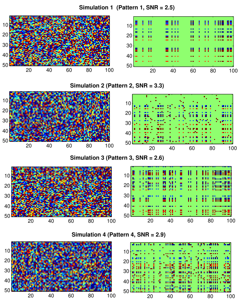
Given a specific pattern mentioned above, we first generate the data matrix. To simulate the real situation, we randomly shuffle the rows and the columns. Next, we add Gaussian noise to each item. Figure 2 illustrates the groundtruth data and the generated data. For each generated data matrix, we also compute the signal to noise ratio (SNR). To illustrate how the methods perform for the data with different SNRs, we further scale down the ground true signal by dividing the original values by 1.2 and 1.5, respectively.
3.1.3 Simulation results
The results of four simulation studies are shown in Figure 3. We use ‘low-rank’ to represent our method as our model is to find biclusters via a low-rank approximation. The details of the simulation results can be found in the supplementary materials. In general, our proposed method achieves comparable performance in the first and third simulation studies and performs better than other three methods in the second and fourth simulation studies. This is because the classical biclustering methods suffer from several limitations, such as missing some entries for overlapped biclusters and the inability to identify the disease/trait-specific entries. Figure 4 shows one result in the fourth pattern. Our proposed method can successfully recover a low-rank component and a sparse component from raw data. In the first simulation, the -scores of sparse biclustering method and SSVD method almost get to 1. The reason why our method performs worse is that we use the default parameters which are not best fit for this simulation set-up. When adjusting the parameters, our method can also get a high -score. Furthermore, we can observe from Figure 3 that our method always perform equally well in terms of both precision and recall while the other three methods often favor precision against recall. In the large-scale data analysis, the conservative method with high precision and low recall may not be suitable for new discoveries because most signals are irrelevant. For such situations, our method has a clear advantage over competitors.

3.2 Real application
We applied our method to analyze 32 independent diseases/traits, including
- •
3 anthropometrics related data.
- •
9 pyschiatry related data.
- •
8 CAD data.
- •
2 social science studies
- •
2 glycaemic traits
- •
7 inflammatory bowel disease data.
- •
systemic lupus erythematosus
- •
parkinson
The details of the data sets including the references and the web link for downloading the data can be found in the supplementary materials. Since each study reports different SNPs, we take the SNPs that are reported by at least 28 diseases/traits and obtain their -values and impute the missing ones. Finally, we get a -value matrix for these 32 diseases/traits. Next, we convert the -value matrix to the -score matrix . We analyze this data set using our method on a desktop PC with 2.40GHz CPU and 4GB RAM. The running time of our method on 32 GWASs data sets is only 152.1s. The three alterative methods investigated in this work cannot be applied due to the large size of the data.
The experiment results are given in Figure 5. The shared causal SNPs are presented in the low-rank component and individual-specific SNPs are shown in the sparse component. We take the first three right singular vectors of the recovered low-rank matrix and use them as the coordinate of each study in Figure 6. From Figure 6, it is clear to see that 3 clusters are recovered from 32 diseases/traits:
- •
2 social science studies (edu_years and college);
- •
diastolic blood pressure and systolic blood pressure (DBP and SBP);
- •
total cholesterol and low density lipoprotein (TC and LDL).
The diseases/traits in each cluster are highly relevant with each other. We compare the identified causal SNPs by our method on 32 GWAS data with some previous findings. For 3 pairs of diseases/traits that are clustered together, we mainly investigate the shared SNPs that are identified by our method. For two social science related data, our method has detected SNP rs3789044, SNP rs12046747, and SNP rs12853561, which are mapped to genes LRRN2 and STK24, respectively. These were reported in the original article [31] because they have significant -values (the details are provided in the supplementary materials). However, besides those SNPs with significant -values, our method has also identified some locus with moderate -values. SNP rs2532269, whose original -values are in edu_years data and in college data, is detected as a causal SNP by our method. This SNP was previously reported (-value ) [32] and mapped to the gene KIAA1267. This gene is highly connected with Koolen-De Vries syndrome. Koolen-De Vries syndrome is characterized by moderate to severe intellectual disability, hypotonia, friendly demeanor, and highly distinctive facial features, including tall, broad forehead, long face, upslanting palpebral fissures, epicanthal folds, tubular nose with bulbous nasal tip, and large ears [33].
For diastolic blood pressure and systolic blood pressure, the identified SNPs in our experiment are also connected with some previously published genes, such as ULK4, FGF5 and C10orf107 [34]. Similarly, some additional locus are identified by the low-rank component. SNP rs4986172 (original -values in SBP data and DBP data are and , respectively), located in the gene ACBD4, is detected by the low-rank component. This gene has been associated with high blood pressure in [35].
To illustrate the power of our method in identifying the causal SNPs that do not shared by several diseases/traits, we take the result of bipolar disorder as an example. The SNPs in the result of bipolar disorder can be matched to ANK3, CACNA1C, SYNE1 and PBRM1, which have been confirmed to be associated with bipolar disorder [36]. The detailed results of other diseases/traits can be found in the supplementary materials. Clearly, the experiment results show that not only can our method recognize SNPs with small -values, but also detect those SNPs with moderate or weak -values.

4 Discussion
Finding weak-effect variants to explain the missing heritability of complex diseases is a challenging task and bottlenecked by the available sample size of GWAS. Based on the fact that related diseases/traits tend to co-occur, discovering shared genetic components among related studies becomes a popular way to address this issue. In the last few years, hundreds of GWASs have been carried out. Therefore, it is timely to systematically investigate GWAS data sets to find those shared patterns for comprehensive understanding of the genetic architecture of complex diseases/traits. In this work, we present a novel method for exploring the genetic patterns of complex diseases. We assume that causal SNPs can be divided into two categories: SNPs shared by multiple diseases/traits and SNPs for individual disease/trait. Thus, by modeling the problem as recovering a low-rank component and a sparse component from a noise matrix, we formulate it as a convex optimization problem. To demonstrate the performance of our proposed method, we conduct several simulation studies under different settings. Simulation results show that the proposed method outperforms three alternative methods in many settings. In the real data studies, we collect 32 large-scale GWAS data sets. We have successively analyzed these data sets via our proposed method and discovered some interesting shared genetic patterns. Many identified variants have been confirmed by other works. To conclude, our proposed method not only possesses a better power than related methods but also provides easily interpretable results for better understanding shared genetic architectures of complex diseases/trais.
In this work, we mainly focus on the analysis of summary statistics. With the development of new technology, more and more supplementary information, such as functional annotation data, structural data, and biochemical data, can be quickly obtained. In the future work, we will integrate these information in our method to increase the statistical power.
Acknowledgments
This work was supported by Georgia State University Deep Grant, Hong Kong Baptist University Strategic Development Fund, Hong Kong Baptist University grant, and Hong Kong Research grant HKBU12202114.
Supplementary Document for “Exploring the genetic patterns of complex diseases via the integrative genome-wide approach”
List
- •
Table S1: 32 GWASs data.
- •
Table S2: 32 GWASs data.
- •
Table S3: Results of four methods when simulations are generated from pattern 1 with different SNRs.
- •
Table S4: Results of four methods when simulations are generated from pattern 2 with different SNRs.
- •
Table S5: Results of four methods when simulations are generated from pattern 3 with different SNRs.
- •
Table S6: Results of four methods when simulations are generated from pattern 4 with different SNRs.
Data descriptions
We applied our method to analyze 32 independent diseases/traits, including
| Name | # of SNPs | Link |
|---|---|---|
| body mass index [37] | 2471516 | http://www.broadinstitute.org/collaboration/giant/index.php/ |
| height [38] | 2469635 | http://www.broadinstitute.org/collaboration/giant/index.php/ |
| crohn’s disease [44] | 953241 | http://www.ibdgenetics.org/downloads.html |
| fasting glucose [43] | 2628879 | http://www.magicinvestigators.org/downloads/ |
| total cholesterol [41] | 2693413 | http://www.sph.umich.edu/csg/abecasis/public/lipids2010/ |
| low density lipoprotein [41] | 2692564 | http://www.sph.umich.edu/csg/abecasis/public/lipids2010/ |
| triglycerides [41] | 2692560 [41] | http://www.sph.umich.edu/csg/abecasis/public/lipids2010/ |
| high density lipoprotein [41] | 2692429 | http://www.sph.umich.edu/csg/abecasis/public/lipids2010/ |
| coronary artery disease [42] | 2420360 | http://www.cardiogramplusc4d.org/downloads/ |
| college [31] | 2321510 | http://ssgac.org/Data.php |
| diastolic blood pressure [34] | 2461325 | http://www.ncbi.nlm.nih.gov/projects/gap/cgi-bin/study.cgi?study\_id=phs000585.v1.p1 |
| systolic blood pressure [34] | 2461325 | http://www.ncbi.nlm.nih.gov/projects/gap/cgi-bin/study.cgi?study\_id=phs000585.v1.p1 |
| eduyears [31] | 2310087 | http://ssgac.org/Data.php |
| fasting Insulin [43] | 2627848 | http://www.magicinvestigators.org/downloads/ |
| multiple sclerosis [45] | 327094 | http://www.ncbi.nlm.nih.gov/projects/gap/cgi-bin/analysis.cgi?study\_id=phs000139.v1.p1\&phv=65549\&phd=1061\&pha=2854\&pht=621\&phvf=\&phdf=\&phaf=\&phtf=\&dssp=1\&consent=\&temp=1 |
| parkinson [51] | 453217 | http://www.ncbi.nlm.nih.gov/projects/gap/cgi-bin/analysis.cgi\?study\_id=phs000089.v3.p2&phv=24040&phd=392&pha=2868&pht=178&phvf=&phdf=&phaf=&phtf=&dssp=1&consent=&temp=1 |
| Name | # of SNPs | Link |
|---|---|---|
| attention-deficit/hyperactivity disorder [13] | 1219805 | http://www.med.unc.edu/pgc/downloads |
| autism spectrum disorder [13] | 1219805 | http://www.med.unc.edu/pgc/downloads |
| bipolar disorder [13] | 1219805 | http://www.med.unc.edu/pgc/downloads |
| major depressive disorder [13] | 1219805 | http://www.med.unc.edu/pgc/downloads |
| schizophrenia [13] | 1219805 | http://www.med.unc.edu/pgc/downloads |
| psoriasis [46] | 440153 | http://www.ncbi.nlm.nih.gov/projects/gap/cgi-bin/analysis.cgi\?study_id=phs000019.v1.p1\&phv=20012\&phd=179\&pha=2855\&pht=63\&phvf=\&phdf=\&phaf=\&phtf=\&dssp=1\&consent=\&temp=1 |
| rheumatoid arthritis [47] | 2556271 | http://www.broadinstitute.org/ftp/pub/rheumatoid\_arthritis/Stahl\_etal\_2010NG/ |
| type 1 diabetes [48] | 503181 | http://www.ncbi.nlm.nih.gov/projects/gap/cgi-bin/analysis.cgi\?study_id=phs000180.v2.p2\&phv=73462\&phd=1548\&pha=2862\&pht=789\&phvf=\&phdf=\&phaf=\&phtf=\&dssp=1\&consent=\&temp=1 |
| type 2 diabetes [2] | 2473441 | http://diagram-consortium.org/downloads.html |
| TagCPD [40] | 2459118 | http://www.med.unc.edu/pgc/downloads |
| TagEVRSMK [40] | 2455846 | http://www.med.unc.edu/pgc/downloads |
| TagFORMER [40] | 2456554 | http://www.med.unc.edu/pgc/downloads |
| TagLOGONSET [40] | 2457545 | http://www.med.unc.edu/pgc/downloads |
| ulcerative colitis [49] | 1428749 | http://www.ibdgenetics.org/ |
| waist-hip ratio adjusted for BMI [39] | 2483326 | http://www.broadinstitute.org/collaboration/giant/index.php/GIANT\_consortium\_data\_files |
| systemic lupus erythematosus [50] | 258402 | http://www.ncbi.nlm.nih.gov/projects/gap/cgi-bin/analysis.cgi?study_id=phs000122.v1.p1&phv=66336&phd=&pha=2848&pht=629&phvf=&phdf=&phaf=&phtf=&dssp=1&consent=&temp=1 |
| SNR = | SNR = | SNR = | ||||||||||
|---|---|---|---|---|---|---|---|---|---|---|---|---|
| Sparsebc | SSVD | LAS | Low-rank | Sparsebc | SSVD | LAS | Low-rank | Sparsebc | SSVD | LAS | Low-rank | |
| Precision | 0.95 | 0.95 | 1 | 0.84 | 0.88 | 0.94 | 1 | 0.75 | 0.71 | 0.92 | 1 | 0.61 |
| Recall | 0.95 | 0.99 | 0.19 | 0.82 | 0.96 | 0.94 | 0.17 | 0.82 | 0.70 | 0.76 | 0.15 | 0.82 |
| F1-score | 0.95 | 0.96 | 0.32 | 0.83 | 0.92 | 0.94 | 0.29 | 0.78 | 0.70 | 0.82 | 0.26 | 0.70 |
| SNR = | SNR = | SNR = | ||||||||||
| Sparsebc | SSVD | LAS | Low-rank | Sparsebc | SSVD | LAS | Low-rank | Sparsebc | SSVD | LAS | Low-rank | |
| Precision | 0.72 | 0.80 | 0.98 | 0.85 | 0.69 | 0.87 | 0.97 | 0.75 | 0.72 | 0.80 | 1 | 0.69 |
| Recall | 0.68 | 0.80 | 0.27 | 0.85 | 0.57 | 0.72 | 0.22 | 0.86 | 0.46 | 0.63 | 0.18 | 0.74 |
| F1-score | 0.69 | 0.80 | 0.42 | 0.85 | 0.61 | 0.79 | 0.36 | 0.80 | 0.56 | 0.71 | 0.30 | 0.71 |
| SNR = | SNR = | SNR = | ||||||||||
|---|---|---|---|---|---|---|---|---|---|---|---|---|
| Sparsebc | SSVD | LAS | Low-rank | Sparsebc | SSVD | LAS | Low-rank | Sparsebc | SSVD | LAS | Low-rank | |
| Precision | 0.99 | 0.74 | 1 | 0.84 | 0.85 | 0.74 | 1 | 0.75 | 0.87 | 0.78 | 1 | 0.77 |
| Recall | 0.61 | 0.79 | 0.29 | 0.86 | 0.63 | 0.79 | 0.22 | 0.84 | 0.56 | 0.69 | 0.22 | 0.75 |
| F1-score | 0.76 | 0.77 | 0.45 | 0.85 | 0.73 | 0.76 | 0.37 | 0.79 | 0.68 | 0.73 | 0.37 | 0.76 |
| SNR = | SNR = | SNR = | ||||||||||
| Sparsebc | SSVD | LAS | Low-rank | Sparsebc | SSVD | LAS | Low-rank | Sparsebc | SSVD | LAS | Low-rank | |
| Precision | 0.86 | 0.76 | 0.99 | 0.80 | 0.81 | 0.85 | 1 | 0.78 | 0.75 | 0.86 | 1 | 0.71 |
| Recall | 0.64 | 0.68 | 0.27 | 0.83 | 0.61 | 0.48 | 0.20 | 0.76 | 0.50 | 0.48 | 0.19 | 0.71 |
| F1-score | 0.72 | 0.72 | 0.43 | 0.82 | 0.69 | 0.62 | 0.23 | 0.77 | 0.59 | 0.62 | 0.32 | 0.71 |
References
- [1] McClellan JM, Susser E, King MC: Schizophrenia: a common disease caused by multiple rare alleles. The British Journal of Psychiatry 2007, 190(3):194–199.
- [2] Morris AP, Voight BF, Teslovich TM, Ferreira T, Segre AV, Steinthorsdottir V, Strawbridge RJ, Khan H, Grallert H, Mahajan A, et al.: Large-scale association analysis provides insights into the genetic architecture and pathophysiology of type 2 diabetes. Nature genetics 2012, 44(9):981.
- [3] Venter JC, Adams MD, Myers EW, Li PW, Mural RJ, Sutton GG, Smith HO, Yandell M, Evans CA, Holt RA, et al.: The sequence of the human genome. science 2001, 291(5507):1304–1351.
- [4] Lander E, Linton L, Birren B, Nusbaum C, Zody M, Baldwin J, Devon K, Dewar K, Doyle M, FitzHugh W, et al.: Initial sequencing and analysis of the human genome. Nature 2001, 409(6822):860–921.
- [5] Sachidanandam R, Weissman D, Schmidt S, Kakol J, Stein L, Marth G, Sherry S, Mullikin J, Mortimore B, Willey D, et al.: A map of human genome sequence variation containing 1.42 million single nucleotide polymorphisms. Nature 2001, 409(6822):928–933.
- [6] Hindorff L, Junkins H, Hall P, Mehta J, Manolio T: A Catalog of Published Genome-Wide Association Studies. Available at: www.genome.gov/gwastudies. Accessed January 22, 2015 2015.
- [7] Manolio T, Collins F, Cox N, Goldstein D, Hindorff L, Hunter D, McCarthy M, Ramos E, Cardon L, Chakravarti A, et al.: Finding the missing heritability of complex diseases. Nature 2009, 461(7265):747–753.
- [8] Maher B: Personal genomes: The case of the missing heritability. Nature 2008, 456(7218):18.
- [9] Yang J, Benyamin B, McEvoy BP, Gordon S, Henders AK, Nyholt DR, Madden PA, Heath AC, Martin NG, Montgomery GW, et al.: Common SNPs explain a large proportion of the heritability for human height. Nature genetics 2010, 42(7):565–569.
- [10] Sivakumaran S, Agakov F, Theodoratou E, Prendergast JG, Zgaga L, Manolio T, Rudan I, McKeigue P, Wilson JF, Campbell H: Abundant pleiotropy in human complex diseases and traits. The American Journal of Human Genetics 2011, 89(5):607–618.
- [11] Vattikuti S, Guo J, Chow CC: Heritability and genetic correlations explained by common SNPs for metabolic syndrome traits. PLoS genetics 2012, 8(3):e1002637.
- [12] Consortium PG, et al.: Genetic relationship between five psychiatric disorders estimated from genome-wide SNPs. Nature genetics 2013.
- [13] Cross-Disorder Group of the Psychiatric Genomics Consortium, et al.: Identification of risk loci with shared effects on five major psychiatric disorders: a genome-wide analysis. Lancet 2013, 381(9875):1371.
- [14] Fisher RA: Statistical methods for research workers 1934.
- [15] Goods I: On the weighted combination of significance tests. Journal of the Royal Statistical Society. Series B (Methodological) 1955, :264–265.
- [16] Stouffer SA, Suchman EA, DeVinney LC, Star SA, Williams Jr RM: The American soldier: adjustment during army life.(Studies in social psychology in World War II, Vol. 1.). 1949.
- [17] Mosteller F, Bush RR, Green BF: Selected quantitative techniques. Addison-Wesley 1970.
- [18] Madeira SC, Oliveira AL: Biclustering algorithms for biological data analysis: a survey. Computational Biology and Bioinformatics, IEEE/ACM Transactions on 2004, 1:24–45.
- [19] Prelić A, Bleuler S, Zimmermann P, Wille A, Bühlmann P, Gruissem W, Hennig L, Thiele L, Zitzler E: A systematic comparison and evaluation of biclustering methods for gene expression data. Bioinformatics 2006, 22(9):1122–1129.
- [20] Busygin S, Prokopyev O, Pardalos PM: Biclustering in data mining. Computers & Operations Research 2008, 35(9):2964–2987.
- [21] Tan KM, Witten DM: Sparse biclustering of transposable data. Journal of Computational and Graphical Statistics 2013, (just-accepted).
- [22] Fazel M: Matrix rank minimization with applications. PhD thesis, Stanford University 2002.
- [23] Candès E, Li X, Ma Y, Wright J: Robust principal component analysis? Journal of the ACM 2011, 58(3):11.
- [24] Tropp JA: Just relax: Convex programming methods for identifying sparse signals in noise. IEEE Transactions on Information Theory 2006, 52(3):1030–1051.
- [25] Boyd S: Distributed Optimization and Statistical Learning via the Alternating Direction Method of Multipliers. Foundations and Trends® in Machine Learning 2010, 3:1–122.
- [26] Cai J, Candès E, Shen Z: A Singular Value Thresholding Algorithm for Matrix Completion. SIAM Journal on Optimization 2010, 20:1956.
- [27] Zhou Z, Li X, Wright J, Candes E, Ma Y: Stable principal component pursuit. In Proceedings of the IEEE International Symposium on Information Theory 2010.
- [28] Meer P, Mintz D, Rosenfeld A, Kim D: Robust regression methods for computer vision: A review. International Journal of Computer Vision 1991, 6:59–70.
- [29] Shabalin AA, Weigman VJ, Perou CM, Nobel AB: Finding large average submatrices in high dimensional data. The Annals of Applied Statistics 2009, :985–1012.
- [30] Lee M, Shen H, Huang JZ, Marron J: Biclustering via sparse singular value decomposition. Biometrics 2010, 66(4):1087–1095.
- [31] Rietveld CA, Medland SE, Derringer J, Yang J, Esko T, Martin NW, Westra HJ, Shakhbazov K, Abdellaoui A, Agrawal A, et al.: GWAS of 126,559 individuals identifies genetic variants associated with educational attainment. Science 2013, 340(6139):1467–1471.
- [32] Consortium EGGE, et al.: Common variants at 6q22 and 17q21 are associated with intracranial volume. Nature genetics 2012, 44(5):539–544.
- [33] Koolen DA, Kramer JM, Neveling K, Nillesen WM, Moore-Barton HL, Elmslie FV, Toutain A, Amiel J, Malan V, Tsai ACH, et al.: Mutations in the chromatin modifier gene KANSL1 cause the 17q21. 31 microdeletion syndrome. Nature genetics 2012, 44(6):639–641.
- [34] International Consortium for Blood Pressure Genome-Wide Association Studies, et al.: Genetic variants in novel pathways influence blood pressure and cardiovascular disease risk. Nature 2011, 478(7367):103–109.
- [35] Newton-Cheh C, Johnson T, Gateva V, Tobin MD, Bochud M, Coin L, Najjar SS, Zhao JH, Heath SC, Eyheramendy S, et al.: Eight blood pressure loci identified by genome-wide association study of 34,433 people of European ancestry. Nature genetics 2009, 41(6):666.
- [36] Chung D, Yang C, Li C, Gelernter J, Zhao H: GPA: A Statistical Approach to Prioritizing GWAS Results by Integrating Pleiotropy and Annotation. PLoS genetics 2014, 10(11):e1004787.
- [37] Speliotes EK, Willer CJ, Berndt SI, Monda KL, Thorleifsson G, Jackson AU, Allen HL, Lindgren CM, Luan J, Mägi R, et al.: Association analyses of 249,796 individuals reveal 18 new loci associated with body mass index. Nature genetics 2010, 42(11):937–948.
- [38] Allen HL, Estrada K, Lettre G, Berndt SI, Weedon MN, Rivadeneira F, Willer CJ, Jackson AU, Vedantam S, Raychaudhuri S, et al.: Hundreds of variants clustered in genomic loci and biological pathways affect human height. Nature 2010, 467(7317):832–838.
- [39] Heid IM, Jackson AU, Randall JC, Winkler TW, Qi L, Steinthorsdottir V, Thorleifsson G, Zillikens MC, Speliotes EK, Mägi R, et al.: Meta-analysis identifies 13 new loci associated with waist-hip ratio and reveals sexual dimorphism in the genetic basis of fat distribution. Nature genetics 2010, 42(11):949–960.
- [40] Tobacco and Genetics Consortium, et al.: Genome-wide meta-analyses identify multiple loci associated with smoking behavior. Nature genetics 2010, 42(5):441–447.
- [41] Teslovich TM, Musunuru K, Smith AV, Edmondson AC, Stylianou IM, Koseki M, Pirruccello JP, Ripatti S, Chasman DI, Willer CJ, et al.: Biological, clinical and population relevance of 95 loci for blood lipids. Nature 2010, 466(7307):707–713.
- [42] Deloukas P, Kanoni S, Willenborg C, Farrall M, Assimes TL, Thompson JR, Ingelsson E, Saleheen D, Erdmann J, Goldstein BA, et al.: Large-scale association analysis identifies new risk loci for coronary artery disease. Nature genetics 2013, 45:25–33.
- [43] Manning AK, Hivert MF, Scott RA, Grimsby JL, Bouatia-Naji N, Chen H, Rybin D, Liu CT, Bielak LF, Prokopenko I, et al.: A genome-wide approach accounting for body mass index identifies genetic variants influencing fasting glycemic traits and insulin resistance. Nature genetics 2012, 44(6):659–669.
- [44] Jostins L, Ripke S, Weersma RK, Duerr RH, McGovern DP, Hui KY, Lee JC, Schumm LP, Sharma Y, Anderson CA, et al.: Host-microbe interactions have shaped the genetic architecture of inflammatory bowel disease. Nature 2012, 491(7422):119–124.
- [45] Fingerprinting G: Risk alleles for multiple sclerosis identified by a genomewide study. N engl J med 2007, 357:851–862.
- [46] Feng BJ, Sun LD, Soltani-Arabshahi R, Bowcock AM, Nair RP, Stuart P, Elder JT, Schrodi SJ, Begovich AB, Abecasis GR, et al.: Multiple loci within the major histocompatibility complex confer risk of psoriasis. PLoS genetics 2009, 5(8):e1000606.
- [47] Stahl EA, Raychaudhuri S, Remmers EF, Xie G, Eyre S, Thomson BP, Li Y, Kurreeman FA, Zhernakova A, Hinks A, et al.: Genome-wide association study meta-analysis identifies seven new rheumatoid arthritis risk loci. Nature genetics 2010, 42(6):508–514.
- [48] Barrett JC, Clayton DG, Concannon P, Akolkar B, Cooper JD, Erlich HA, Julier C, Morahan G, Nerup J, Nierras C, et al.: Genome-wide association study and meta-analysis find that over 40 loci affect risk of type 1 diabetes. Nature genetics 2009, 41(6):703–707.
- [49] Anderson CA, Boucher G, Lees CW, Franke A, D’Amato M, Taylor KD, Lee JC, Goyette P, Imielinski M, Latiano A, et al.: Meta-analysis identifies 29 additional ulcerative colitis risk loci, increasing the number of confirmed associations to 47. Nature genetics 2011, 43(3):246–252.
- [50] Hom G, Graham RR, Modrek B, Taylor KE, Ortmann W, Garnier S, Lee AT, Chung SA, Ferreira RC, Pant PK, et al.: Association of systemic lupus erythematosus with C8orf13–BLK and ITGAM–ITGAX. New England Journal of Medicine 2008, 358(9):900–909.
- [51] Simon-Sanchez J, Schulte C, Bras JM, Sharma M, Gibbs JR, Berg D, Paisan-Ruiz C, Lichtner P, Scholz SW, Hernandez DG, et al.: Genome-wide association study reveals genetic risk underlying Parkinson’s disease. Nature genetics 2009, 41(12):1308–1312.