Combining synchrosqueezed wave packet transform with optimization for crystal image analysis
Abstract
We develop a variational optimization method for crystal analysis in atomic resolution images, which uses information from a 2D synchrosqueezed transform (SST) as input. The synchrosqueezed transform is applied to extract initial information from atomic crystal images: crystal defects, rotations and the gradient of elastic deformation. The deformation gradient estimate is then improved outside the identified defect region via a variational approach, to obtain more robust results agreeing better with the physical constraints. The variational model is optimized by a nonlinear projected conjugate gradient method. Both examples of images from computer simulations and imaging experiments are analyzed, with results demonstrating the effectiveness of the proposed method.
Keywords:
Atomic crystal images, crystal defect, elastic deformation, D synchrosqueezed transforms, optimization1 Introduction
Defects, like dislocations, grain boundaries, vacancies, etc., play a fundamental role in polycrystalline materials. They greatly change the material behavior from a perfect crystal and affect the macroscopic properties of the materials. Analysis of images arising from atomistic simulations or imaging of polycrystalline materials hence becomes very important to characterize and help understand the defects and their effects on crystalline materials. While the defect analysis is traditionally done by visual inspection, the large amount of data made available due to advances in imaging and simulation techniques creates a need of efficient computer-assisted or automated analysis.
Crystal deformation at the atomic scale is another important quantity that characterizes polycrystalline materials. When the deformation, denoted by , is well-defined, the tensor field describes the local crystal strain; the polar decomposition of at each point gives grain rotations; the curl of provides information about defects and the well-known Burgers vector that represents the magnitude and direction of the lattice distortion resulting from a dislocation. Since it is almost impossible to estimate the deformation manually, the development of computer-aided analysis becomes important.
For crystalline materials, defects are physical domains of the materials such that it is not possible to identify a smooth crystal deformation that maps the atomic configuration back to a perfect lattice. In other words, the deformation gradient is irregular and has nonzero curl at the defect location. In the opposite case, when a smooth deformation map does exist, the affine transform given by the gradient of the map, , transforms the image locally to an undistorted lattice of atoms. Therefore, for a defect-free region of the material, is a gradient field and thus is curl-free: . Crystal image analysis hence requires the detection of the defect regions and preferably also the estimation of the local elastic deformation away from the defects.
In recent years several variational image processing methods for crystal analysis have emerged. The most basic versions just segment the crystal image into several crystal grains and identify their orientation, using clever formulations as convex optimization in D [3, 11] or efficient, sophisticated optimization algorithms for D images [9]. Berkels et al. additionally determine a full deformation field [2] via nonlinear optimization, while defects and local crystal distortion are identified in [8].
If accurate atom positions can easily be extracted from the image (or if the data stems from atomistic simulations) such that the input data consists of a discrete list of atom positions, then the local lattice orientation and deformation as well as defects can be obtained efficiently by identifying the nearest neighbors of each atom [12, 13, 1].
Another efficient approach is the crystal image analysis via D synchrosqueezed transforms (SSTs) in [16]. The SST was originally proposed in [5], rigorously analyzed in [4, 14, 15], and extended to D in [17, 19]. It is proved that the D SST can accurately estimate the local wave vector of a nonlinear wave-like image. Inspired by the fact that a deformed atomic crystal grain can be considered as a superposition of several nonlinear wave-like components, [16] proposes an efficient crystal image analysis method based on a D band-limited SST. In particular, tracking the irregularity of the synchrosqueezed energy can identify defects, and the deformation gradient can be obtained by a linear system generated with local wave vector estimations. A recent paper [18] on the robustness of SSTs supports the application of this analysis method to noisy crystal images. The idea of exploiting the local periodic structure in the Fourier domain to extract a deformation gradient has also been considered in [10] in the crystal imaging literature.
Our work here is a variational approach based on the information obtained from a band-limited D synchrosqueezed wave packet transform following [16]. In this manuscript, we use this information as input to a variational optimization in order to improve the robustness of the analysis and, importantly, to make the results better agree with the physical nature of defects.
2 Variational method to retrieve deformation gradients
Let us fix a perfect, unstrained crystal with a fixed orientation as our reference lattice. Let be the domain of the image. Our objective is to find at each the local strain or deformation gradient of a (locally defined) deformation which deforms a defect-free neighborhood of into the reference lattice. (Note that since the image corresponds to a deformed crystal state, should be understood as an Eulerian coordinate.) In other words, we seek the affine map defined by which maps the local atom arrangement to the reference lattice. This is however impossible around defects. In particular, while in the elastic region, in the defect region, is not zero, and the integral of over a neighborhood of the defect such as a dislocation should match the defect’s Burgers vector [9].
Assume the defect region is given by and the curl of G is given by , consistent with the Burgers vectors and with on . We expect the displacement field to minimize the elastic energy of the system outside the defect region, since the system under imaging is in a quasistatic state. Given a rough guess of the deformation gradient, this motivates the energy minimization
| (1) | ||||
where denotes the Frobenius norm of a matrix, , and is the elastic stored energy density.
Since our reference lattice represents the undeformed equilibrium state of the crystal and the atom configuration in the image is produced by the (local) deformation , the stored elastic energy can be expressed in the standard Lagrangian form as the integral over the reference domain of an elastic energy density that depends on ,
Here, satisfies the standard conditions coming from first principles, i. e. is frame indifferent, for , else, and if . After a change of variables the elastic energy turns into
for , where it is easy to see that has the same above properties as . For (or equivalently ) one can use a material-specific, possibly anisotropic energy density. To be specific, since our numerical examples are all concerned with a triangular lattice exhibiting isotropic elastic behavior, we here simply restrict ourselves to the following neo-Hookean-type elastic energy density
| (2) | ||||
Note that in (1), the fidelity and elastic energy terms are both evaluated outside the defect region. Within the defect region, since it is not possible to map the local configuration of atoms back to the reference state, the estimate is not trustworthy. It is also well known that the elastic energy blows up logarithmically approaching the dislocation core, and hence it only makes sense to penalize the elastic energy away from the defects.
The questions are then how to estimate and to determine the defect region as well as the vector field consistent with the defects’ Burgers vectors. In this work, the desired information is all obtained using synchrosqueezed wave packet transforms. We first review the synchrosqueezed wave packet transforms and the estimate of in §2.1. The defect region and Burgers vectors are estimated using the synchrosqueezed wave packet transforms as explained in §2.2. The variational problem (1) is then solved by a constrained minimization algorithm as described in §2.3.
2.1 Synchrosqueezed wave packet transforms (SSTs)
Before explaining the variational optimization, we briefly introduce the crystal image model established in [16] and the synchrosqueezed wave packet transforms in [17, 19] for the purpose of a self-contained description. Consider an image of a polycrystalline material with atomic resolution. Denote the perfect reference lattice as
where represent two fixed lattice vectors. Let be the image corresponding to a single perfect unit cell, extended periodically in with respect to the reference crystal lattice. We denote by the domain occupied by the whole image and by , , the grains the system consists of. Now we model a polycrystal image as
| (3) |
where is the reciprocal lattice parameter (or rather the relative reciprocal lattice parameter as we will normalize the dimension of the image). The is chosen to map the atoms of grain back to the configuration of a perfect crystal, in other words, it can be thought of as the inverse of the elastic displacement field. The local inverse deformation gradient is then given by in each . For generality, (3) also includes a smooth amplitude envelope and a smooth trend function to take into account possible variation of intensity, illumination, etc. during the imaging process. Using the Fourier series of and the indicator functions , we can rewrite (3) as
| (4) |
where is the reciprocal lattice of (recall that is periodic with respect to the lattice ). In each grain , the image is a superposition of wave-like components with local wave vectors and local amplitude . Our goal here is to apply the band-limited D SST developed in [16] to estimate the defect region and also in the interior of each grain as required in the variational formulation.
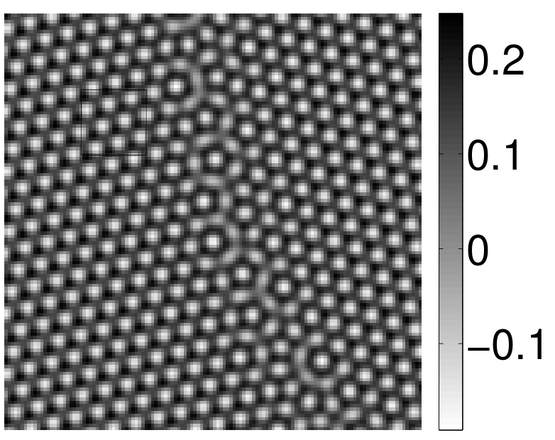
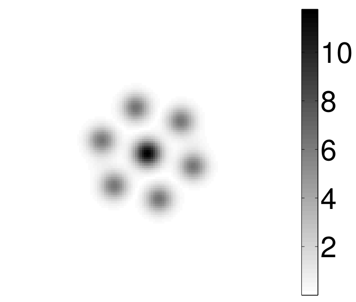
The starting point of D SST is a wave packet , which is, roughly speaking, obtained by translating, rotating, and rescaling or modulating a mother wave packet according to the parameters , , and [17, 19, 16]. Let be the wave packet transform of at scale and angle in the frequency domain, and at spatial location . The wave packet transform is a generalization of curvelet and wavelet transforms with better flexibility in frequency scaling and consequently is better suited to analyze crystal images with complex geometry. As a convolution with smooth wave packets, is well-defined and smooth even under very low regularity requirements for , e. g. . The spectrum of the windowed Fourier transform of a given crystal image spreads out in the phase space, as illustrated in Figure 1(b). The D synchrosqueezed wave packet transform (SST) aims at sharpening this phase space representation. In the SST, for each , we define the corresponding local wave vector
Here, denotes the gradient of with respect to its third argument . The synchrosqueezed (SS) energy distribution of is then constructed as
| (5) |
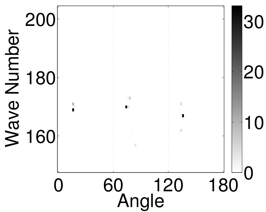
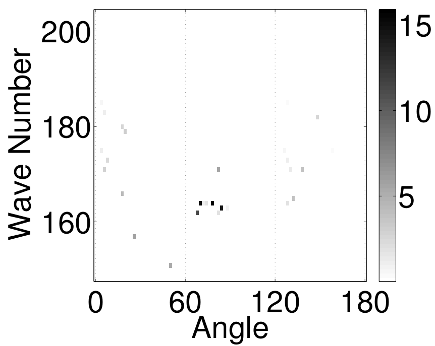
where denotes the Dirac measure. By the stationary phase method, in a small neighborhood of a point such that is nonzero for some fixed , is essentially a plane wave in with a local wave vector approximating a certain . Inspired by this intuition, it is proved in [16] that in the interior of a grain, the local wave vector estimation approximates local wave vectors accurately, if the deformation and the amplitude function are smooth. The SST squeezes the wave packet spectrum according to to obtain a sharpened and concentrated representation of the image in the phase space. Hence, in the interior of a grain, the SS energy distribution has a support concentrating around local wave vectors , , and is given approximately by (see e.g., Figure 1(e) in polar coordinates)
| (6) |
understood in the distributional sense. Therefore, by locating the energy peaks of , we can obtain estimates of local wave vectors and also their associated spectral energy. In practice, we will aim at high energy peaks corresponding to close to the origin in the reciprocal lattice. For simplicity and concreteness, we will in this article focus on the case when the lattice is hexagonal. We then have six such reciprocal lattice vectors , which can be further reduced to three due to the symmetry . We will henceforth denote these as , , and denote by the estimate of . The inverse deformation gradient is determined by a least squares fitting of the deformed reference reciprocal lattice vectors to the :
In practice, for each physical point we represent in polar coordinates (where is ignored due to symmetry). To identify the peak locations , we choose the grid point with highest amplitude in each degree sector of .
As the representation (6) of is no longer valid around the crystal defects, we may characterize the defect region by using an indicator function for the deviation of from the representation (6). To this end, for each (corresponding to one of the sectors), we define
where denotes a small ball around the estimated local wave vector . Hence, will be close to in the interior of a grain due to (6), while its value will be much smaller than near the defects. This is illustrated in Figure 1(c), where we show for the crystal image in Figure 1(a). The estimate of defect regions can be obtained by a thresholding at some value according to
an illustration of which is shown in Figure 1(d). Figure 2 shows the estimate of by the SST. It is observed that the crystal is slightly deformed in the grain interior and heavily deformed at the defect region.
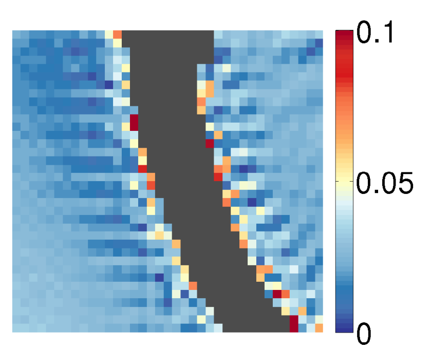
To better interpret the inverse deformation gradient , we compute its polar decomposition for each point , where is a rotation matrix and is a positive-semidefinite symmetric matrix. The rotation angle of describes the crystal orientation at ; indicates the volume distortion of ; the quantity , where and are the eigenvalues of , characterizes the difference in the principal stretches of as a measure of shear strength. The bottom panel of Figure 2 shows these quantities corresponding to the estimate of in the top panel. In the later numerical examples, instead of itself we will always present the crystal orientation, the volume distortion, and the difference in principal stretches.
 |
 |
| (a) | (b) |
| (c) | (d) |
 |
 |
| (e) | (f) |
 |
 |
| Crystal Orientation | Difference in principal stretches |
 |
| Volume Distortion |
2.2 Defect region, topological consistency, and Burgers vector identification
Based on the estimated , we can determine the defect region and also the Burgers vectors or equivalently the curl field used in the constraint of our variational formulation (1). We give the details in this section.
2.2.1 Burgers vectors and
As explained previously, away from defects, can be interpreted as the gradient of a (fictitious) deformation deforming the configuration of the given image into a perfect reference crystal of a fixed orientation. Now the fact that gradient fields are always curl-free can be exploited as a constraint
| (7) |
in the variational method. In the defect region , however, the interpretation of as a deformation gradient breaks down since there is no smooth deformation of the crystal that can undo the lattice defect. In fact, denoting the connected components of by , it is relatively simple to see that the integral
| (8) |
is the Burgers vector associated with the defect in . Indeed, consider any closed injective curve that encloses counterclockwise, but does not intersect . Figure 3, left, shows a specific example of such a curve, which is chosen such that it connects a sequence of neighboring atoms. Denote the curve interior by . Since lies in the defect-free region, for every there is a deformation (the gradient of which is given by ) that deforms a neighborhood of into the perfect reference configuration of the crystal. Starting at we can thus iteratively map little segments of the curve into the reference crystal via , resulting in a curve on the reference configuration. Note that is in general no longer closed or injective. By Stokes’ Theorem, using the tangent vector to , we have
The vector on the right-hand side is the defect’s Burgers vector and is obviously independent of the originally chosen curve . If contains an isolated dislocation surrounded by a regular lattice, just represents the Burgers vector of that dislocation. If contains multiple dislocations or even a section of a high angle grain boundary, represents the accumulated Burgers vector of all defects in (note that a high angle grain boundary may be thought of as a string of dislocations with distance smaller than the lattice spacing so that the single dislocations are not clearly spatially separated; Figure 6(c) gives an impression of the size of the numerically found .

As in the case of , where we know , we also have a priori information on in . In particular we know that is a Burgers vector and thus must lie in the discrete set of Bravais lattice vectors of the perfect reference lattice . We thus identify by projecting the (potentially noisy) estimate onto and then impose (8) as a constraint on . In fact, instead of prescribing the accumulated curl in via (8) we may just as well prescribe
| (9) |
for a function with (in mathematically more precise terms, may be a distribution). This is possible since we are only interested in the field outside of and since any field satisfying (7) and (8) can be modified on to a field satisfying (9). The function is here simply chosen as with such that (i.e., an overall scaling of ). Summarizing, in our variational method to extract from the noisy data we will prescribe the constraint
| (10) |
2.2.2 Refined defect regions
On the one hand, the threshold to identify should be chosen very low to yield thin and localized defect regions (e. g. such that defect regions around single dislocations stay separated from each other), on the other hand, the thinner the identified defect region the worse will the estimate of the Burgers vectors be. A compromise is to first use thick defect regions in order to estimate the Burgers vectors and then to impose the constraint (10) with a much finer estimate of the . However, it may happen that a thick patch contains multiple thin connected components . In that case the are defined as the closest projections of onto under the constraint , where is the accumulated Burgers vector of the patch . In order to obtain a very thin and localized we simply identify the ridge of inside the thick and then dilate this ridge by a few pixels. The ridge computation turns out to be sufficiently robust even in the presence of noise, as can be seen from the similarity between the detected defect regions with and without noise in Figures 6 and 7.
2.2.3 Introduction of jump sets for topological consistency
A Bravais lattice does typically not only exhibit translational, but also rotational symmetry. The so-called point group comprises all those rotations which leave the reference lattice invariant. This leads to an ambiguity in the deformation gradient : if correctly describes the local configuration of the crystal, then for any does so as well. Even though the constraint (10) has the effect that the matrix field will be locally consistent (in the sense that for any in a neighborhood of we have ), global consistency is often not guaranteed. Indeed, Figure 4 shows a situation in which along a closed path , changes continuously from the identity to an element of the point group. Since describes the same local crystal configuration as , the curl where jumps from to is spurious. As in [8], this inconsistency can be remedied by introducing a cut set across which the tangential component of is allowed to jump by a point group element,
for some , where and denote the value of on either side of and denotes the tangent to .
Note that we have large freedom to choose the cut set . For instance we could take to be composed of smooth lines connecting the different connected components of . Those lines can easily be chosen in such a way that they do not intersect and that the connected components, say , of are simply connected. Within each , the crystal is defect-free, thus there is a deformation mapping onto the reference crystal. The matrix field will be the gradient of inside , which is automatically consistent all over . If jumps across between two neighboring components and , then for all we must have with a constant , since lies inside a defect-free crystal region ( and denote the value of in and , respectively, while is the tangent vector to ). Therefore, not only is smooth, but even constant on each curve segment of . Furthermore, up to multiplications with point group elements, the optimal does not depend on the particular position and geometry of . Indeed, if is shifted, producing new , , , then the new optimal field is given by
For simplicity, the cut set in our computation is algorithmically chosen after the problem discretization. First we sweep over all image pixels and reassign the pixel values via a fast marching type method. Let denote the set of already treated pixels (consisting initially of only one pixel). Amongst the not yet treated neighbors of all pixels in , we pick the pixel with the smallest value of , where denotes the neighboring pixel. We replace its value with for the minimizer and set . After all pixels have been swept through in this way, we set to be the union of interfaces between neighboring pixels that have . Note that we also take care that so that the estimation of Burgers vectors is not impaired.
2.2.4 Variational principle with topological jump set
While we will use on the whole domain in the numerical algorithm, as the energy (1) depends only on on , it is more convenient to reformulate the problem with a bounded Lipschitz domain and consider the Hilbert space
| (11) |
with norm given by
| (12) |
Note that , where we recall that are the connected components of . We define the tangential trace operators and on the two sides of for as
| (13) |
where is the unit normal of and . It is standard (see e. g., [6]) using Green formula that can be extended to bounded linear operators from to the fractional Hilbert space . Similarly, we may also define the trace operator on .
For the (inverse) deformation gradient , it is then natural to consider the space as the rows of : and lie in . Thus, we generalize the tangential trace operators and also to , such that they act on each row of and map to and , respectively. In particular, as we are only concerned with on , the constraint on is equivalent to .
With this, we may formulate (1) with the topological jump set more precisely as
| (14) | ||||
| s. t. | ||||
for some fixed piecewise constant . Here the last equation is understood in the space of (this is well defined as for any due to the regularity of ).
Theorem 1.
Assume that the topological jump set and the boundary of are Lipschitz. Given , piecewise constant, and a finite measure on , the minimizer to the variational problem (14) exists.
Proof.
We consider the admissible space of :
Note that this is a closed linear subspace of , and hence any bounded sequence is weakly compact in . Given a minimizing sequence of (14), as the energy is uniformly bounded, we have
for some constant . Together with , we obtain that is uniformly bounded, and hence weakly convergent (in ) to . The existence then follows from the lower semi-continuity of and with respect to the weak topology (which is clearly weaker than the weak topology of ). ∎
2.3 Constrained minimization algorithm
In this section we describe the numerical algorithm to solve the minimization problem (1) or rather the corresponding version with topological jump set (14). It is more convenient to describe the algorithm for the following simplified formulation, which is equivalent after discretization.
| (15) | ||||
| s. t. |
where and denote the value of on either side of . For simplicity we use the same notation for the continuous and discrete objects.
2.3.1 Finite difference discretization
The image domain is discretized via Cartesian pixels, indexed by --position (the pixel spacing is assumed to be one). For an index we denote by and the next larger or next smaller index, where for simplicity we assume periodic boundary conditions and use cyclic indexing, i. e. , , , for all . The matrix fields are discretized accordingly, . The jump set follows the edges between the pixels and is represented as a collection of horizontal or vertical pixel pairs, . Furthermore, we define the function such that is the point group element with smallest distance to . is extended to by the identity in . Derivatives in - and -direction are replaced by finite differences that respect the point group equivalence across ,
where superscript denotes the -matrix entry. Throughout, a superscript denotes discrete differential operators. In particular, the discrete curl and Laplacian are defined as
where denotes the th column of the matrix and the superscript denotes the adjoint operator, which in this particular case is given by
2.3.2 Projected descent in constraint space
The discrete optimization problem reads
The constraint space is an affine space and can be expressed as for a with . Hence, the energy can be minimized using a standard projected nonlinear conjugate gradient (NCG) descent in . In more detail, we employ a Fletcher–Reeves NCG method in which the derivative of with respect to is always orthogonally projected onto (i. e. onto its component parallel to ) so that the algorithm is performed within the subspace . Due to accumulating numerical errors we also have to project the current estimate back onto from time to time. Denoting the projection onto by , the NCG algorithm is initialized with .
The projection is the solution to the constraint minimization , which satisfies the optimality conditions
for a Lagrange multiplier . Applying to the second equation we obtain
Note that . Denoting by the inverse of , we obtain and thus
Once is computed, the projection onto can also be obtained as
2.3.3 Fast projection onto constraint space
For the above projection we need to invert the discrete Laplacian operator. Using periodic boundary conditions this would be very fast using FFT if there was no jump set . However, with nonempty jump set , our finite difference operators do not turn into pointwise multiplications in Fourier space. In order to obtain a fast inversion we decompose , where is the standard discrete Laplacian and the linear operator accounting for the point group,
Note that is symmetric, and it is highly sparse and thus has a very small range and a large kernel . If we decompose into
then we obtain
| (16) |
The solvability condition tells us that is orthogonal to the right-hand side, so we can just as well project the right-hand side onto by subtracting the mean,
Now choosing a basis and , we write
where denotes the inverse of . The degrees of freedom now have to satisfy the equations , , (due to ) and , , (the solvability condition for (16)) where the dot denotes the dot product. In detail, the equations are given by
| (17) |
To solve for , we write the linear system as a matrix vector equation. Since we need to solve systems of the form several times for different values of , we perform a QR decomposition,
where is a permutation matrix such that the lower rows of are zero (this is possible since the solution to is only uniquely specified up to a two-dimensional subspace due to ) and all other rows have nonzero diagonal elements. Note that this decomposition is the bottleneck of the algorithm with a complexity of . The degrees of freedom corresponding to the zero-rows can now be chosen freely (say, as zero), and the resulting
solves . Note that can readily be computed via FFT and that the can be chosen as shifted versions of , , with except for the th entry of being one. Thus, can be evaluated efficiently as just a shift of .
3 Numerical results
In this section, we present several numerical examples for images coming from both computer simulations and real experiments to illustrate the performance of our method. The corresponding code is open source and available as SynCrystal at https://github.com/SynCrystal/SynCrystal. We first apply our method to analyze synthetic crystal images of phase field crystals (PFC) [7]. To show the robustness of our method, both noiseless and noisy examples of PFC images are presented. Moreover, we examine different kinds of crystal images from real experiments: (1) a TEM-image of GaN with a series of isolated defects that leads to a large angle grain boundary; (2) a photograph of a bubble raft with a thick transition region at grain boundaries; (3) a TEM-image of Al with a noisy and irregular grain boundary.
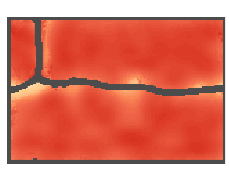
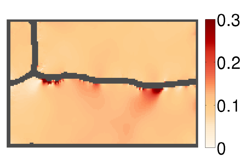
In all of these examples, we compare the initial estimated strain provided by the SST-based analysis described in §2.1 and the improved results from the variational method (15), where each time we display crystal orientations, difference in principal stretches, and volume distortion. For better visualization we mask out the identified defect regions (in which there is no meaningful notion of strain). The curl of (which in general violates the physical constraint of being zero outside and of being compatible with the defects’ Burgers vectors) as well as the average per connected defect region (which is compatible with the defects’ Burgers vectors) are also shown.
The main parameters for the SST-based analysis are two geometric scaling parameters and in the 2D SST (for details see [18]). Smaller scaling parameters result in better robustness of SSTs while larger scaling parameters give more accurate estimates in noiseless cases [18]. Hence, we adopt in the examples with less noise and use when the crystal image is noisy. As discussed in [18], for images with heavy noise, the synchrosqueezed transform can still provide reasonable initial guess via a highly redundant transform with more computational cost. The variational model parameters and in (2) are simply set to in all of the following examples.
During the synchrosqueezed transform we also downsample the original image in the frequency domain and reduce the mesh size for the variational optimization. As a result, the computational mesh of the optimization model is actually independent of the resolution of the crystal images. To achieve a short computation time, we typically choose the downsampling rate as large as possible such that defects can still be localized with a precision below one atom spacing. Figure 8 will show a comparison between different downsampling rates.
The main computational cost arises from inverting the Laplace operator via the solution of (17). The number of variables is proportional to the number of pixel pairs of the singularity set , and the solution cost scales like . Note that, since has codimension , behaves roughly like the number of image pixels along one direction (and not like the total number of pixels), so the computations are still feasible for quite large images. The runtime for the examples in Figure 9 is less than seconds, the runtime for the PFC image in Figure 5, left, is seconds. The runtime for the example in Figure 12 with heavy noise is about minute due to extra effort to obtain robustness of the synchrosqueezed transform.
3.1 Synthetic crystal images
 |
 |
  |
  |
| (a) | (b) |
  |
  |
| (c) | (d) |




 |
 |
 |
 |
 |
 |
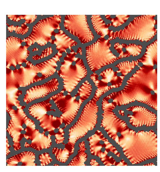
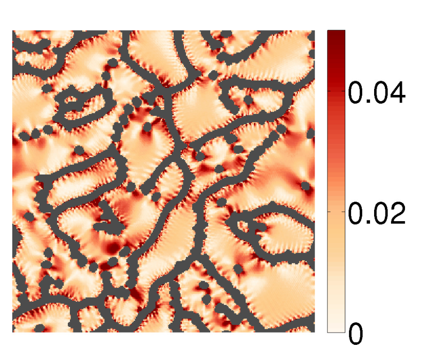
The PFC model is a well-established method to simulate elastic and plastic deformations, free surfaces, and multiple crystal orientations in nonequilibrium processes. Its simulation can provide synthetic crystal images with various topological defects. A noiseless PFC image is given in Figure 5 (left). It contains isolated defects and large as well as small angle grain boundaries, the latter showing up as a string of dislocations.
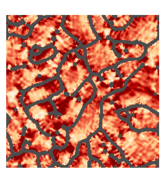
Compared to the initial strain estimate , the optimized is smoother, exhibits a much smaller overall volume distortion and shear (as visualized by the difference in principal stretches), and sharpens the compression-dilation dipoles around each single dislocation, as shown in Figure 6.
The noisy PFC image of Figure 5 (right) is generated by adding 50 Gaussian random noise. Obviously, this leads to strong artifacts in the estimated deformation . Remarkably, after the optimization we retrieve an estimate almost as good as in the noiseless case as shown in Figure 7, which demonstrates the robustness of our method.
To show that the performance of our method is not really depending on the mesh size chosen for the optimization algorithm, we compare the results obtained with different downsampling rates in the synchrosqueezed transform. Figure 8 summarizes the comparison for the PFC example. Even though the grain boundary geometry is complicated in this example, our algorithm obtains similar results for different downsampling rates.
3.2 Experimental crystal images
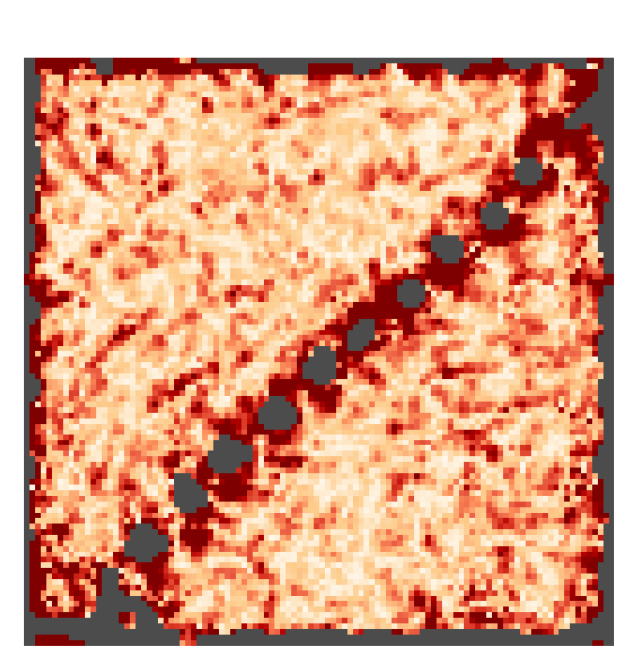
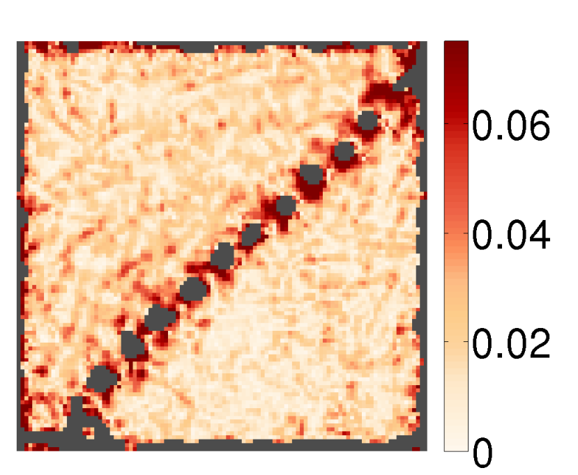
The first real crystal image, a TEM-image of GaN of size (Figure 9 left), contains a string of dislocations forming a large angle grain boundary. The artificial strong spatial variation of crystal orientation, shear and volume distortion in the SST result is greatly reduced after applying the optimization as shown in Figure 10. Even more importantly, the unphysical curl away from the defects is completely removed such that the curl of is fully concentrated in the single defect regions around each dislocation (the total curl of each region equalling the dislocation’s Burgers vector).
 |
 |
  |
  |
  |
  |
  |
  |
  |
  |
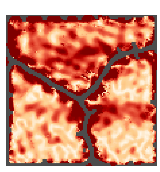
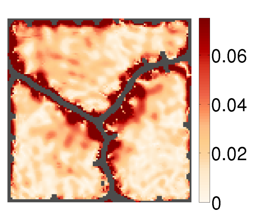
The second example is a photograph of a bubble raft with strongly disordered and blurry grain boundaries (Figure 9 right). The image size is pixels. The SST result (see Figure 11) shows a spurious strong shear of the local crystal structure close to the grain boundaries, especially near the triple junction. One of the reasons for this behavior is that the SST, like any wavelet type transform, extracts directional and strain information from image patches, which here have to be larger than the unit cells. Thus, the grain boundaries are diffused, and information near the grain boundary is not trustworthy. The optimization can mostly remedies this effect.
The last experimental example is a TEM-image of a twin and a high angle grain boundary in Al (Figure 12). The image size is pixels. The crystal structures in each grain are also slightly stretched. Although this example is very challenging, the SST-based analysis can still provide an accurate defect region estimate and a reasonable initial guess (see Figure 13). After optimization, we obtain a curl-free inverse deformation gradient in the grain interior. The difference of principal stretches becomes smaller and the volume distortion gets closer to zero outside the defect region.
 |




4 Discussion
We have presented a variational method to improve an initial analysis of a crystal image provided by the SST-based method developed in [16]. By minimizing the elastic energy of the local inverse deformation gradient outside the SST-estimated defect region, we obtain an optimized deformation gradient that better agrees with physical understanding. The desired information about the local crystal state is immediately available from : the polar decomposition of gives crystal orientations; the determinant of indicates volume dilation and compression; the curl of indicates defect regions, etc.
The variational method in this paper presents a first step towards regularizing the local inverse deformation gradient provided by SST. In this step, we only focus on the optimization outside defect regions. In a next step, one has to investigate variational models to also obtain a meaningful estimate of the deformation gradient inside defect regions, which would provide a more accurate localization of defects. One possible solution could be a nested optimization model with an inner and an outer loop, where the inner loop performs the optimization outside the defect regions as proposed in this paper. The outer loop then tries to improve inside the defect regions. We will leave this to future works.
Acknowledgment
The work of J.L. was supported in part by the Alfred P. Sloan foundation and National Science Foundation under award DMS-1312659. B.W.’s research was supported by the Alfried Krupp Prize for Young University Teachers awarded by the Alfried Krupp von Bohlen und Halbach-Stiftung. H.Y. was partially supported by Lexing Ying’s grants: the National Science Foundation under award DMS-1328230 and the U.S. Department of Energys Advanced Scientific Computing Research program under award DE-FC02-13ER26134/DE-SC0009409. The authors thank Lexing Ying for helpful suggestions and comments.
References
- [1] C. Begau, J. Hua, and A. Hartmaier. A novel approach to study dislocation density tensors and lattice rotation patterns in atomistic simulations. J. Mech. Phys. Solids, 60(4):711–722, 2012.
- [2] B. Berkels, A. Rätz, M. Rumpf, and A. Voigt. Extracting grain boundaries and macroscopic deformations from images on atomic scale. J. Sci. Comput., 35:1–23, 2008.
- [3] M. Boerdgen, B. Berkels, M. Rumpf, and D. Cremers. Convex relaxation for grain segmentation at atomic scale. In Vision, Modeling, and Visualization, pages 179–186. Eurographics Association, 2010.
- [4] I. Daubechies, J. Lu, and H.-T. Wu. Synchrosqueezed wavelet transforms: an empirical mode decomposition-like tool. Appl. Comp. Harmonic Anal., 30:243–261, 2011.
- [5] I. Daubechies and S. Maes. A nonlinear squeezing of the continuous wavelet transform based on auditory nerve models. In Wavelets in Medicine and Biology, Ed. A. Aldroubi and M. Unser, pages 527–546. CRC Press, 1996.
- [6] G. Duvaut and J. L. Lion. Les inéquations en Mécanique et en Physique (English Translation). Springer-Verlag, New York, 1977.
- [7] K. R. Elder and M. Grant. Modeling elastic and plastic deformations in nonequilibrium processing using phase field crystals. Phys. Rev. E, 70:051605, 2004.
- [8] M. Elsey and B. Wirth. Fast automated detection of crystal distortion and crystal defects in polycrystal images. Multi. Model. Simul., 12:1–24, 2014.
- [9] M. Elsey and B. Wirth. Redistancing dynamics for vector-valued multilabel segmentation with costly fidelity: grain identification in polycrystal images. J. Sci. Comp., pages 1–28, 2014.
- [10] M. Hÿtch, E. Snoeck, and R. Kilaas. Quantitative measurement of displacement and strain fiedls from HREM micrographs. Ultramicroscopy, 74:131–146, 1998.
- [11] E. Strekalovskiy and D. Cremers. Total variation for cyclic structures: Convex relaxation and efficient minimization. In Computer Vision and Pattern Recognition (CVPR), 2011 IEEE Conference on, pages 1905–1911, 2011.
- [12] A. Stukowski and K. Albe. Dislocation detection algorithm for atomistic simulations. Model. Simul. Mater. Sci. Eng., 18:025016, 2010.
- [13] A. Stukowski and K. Albe. Extracting dislocations and non-dislocation crystal defects from atomistic simulation data. Model. Simul. Mater. Sci. Eng., 18:085001, 2010.
- [14] G. Thakur and H.-T. Wu. Synchrosqueezing-based recovery of instantaneous frequency from nonuniform samples. SIAM J. Math. Anal., 43(5):2078–2095, 2011.
- [15] H. Yang. Synchrosqueezed wave packet transforms and diffeomorphism based spectral analysis for 1D general mode decompositions. Appl. Comp. Harmon. Anal., in press.
- [16] H. Yang, J. Lu, and L. Ying. Crystal image analysis using 2D synchrosqueezed transforms, 2014. preprint, arXiv:1402.1262 [math.NA].
- [17] H. Yang and L. Ying. Synchrosqueezed wave packet transform for 2D mode decomposition. SIAM J. Imaging Sci., 6:1979–2009, 2013.
- [18] H. Yang and L. Ying. Robustness analysis of synchrosqueezed transforms, 2014. preprint, arXiv:1410.5939 [math.ST].
- [19] H. Yang and L. Ying. Synchrosqueezed curvelet transform for two-dimensional mode decomposition. SIAM J. Math. Anal., 46(3):2052–2083, 2014.