跳到论文正文
W Papers独立论文阅读器 arXiv:1501.06003 论文正文 计算阅读时间 · 0%
引用这篇论文根据当前论文元数据生成,正式投稿前建议核对。


License: arXiv.org perpetual non-exclusive license
arXiv:1501.06003v2 [cs.IT] 15 Feb 2016

Improved Lower Bounds for Coded CachingThanks: The material in this work has appeared in part at the 2015 IEEE International Symposium on Information Theory.

Hooshang Ghasemi and Aditya Ramamoorthy Affiliation: Dept. of Electrical & Computer Eng.
Iowa State University, Ames, IA 50011
Email: {ghasemi, adityar}@iastate.edu
Affiliation: 
Abstract

Content delivery networks often employ caching to reduce transmission rates from the central server to the end users. Recently, the technique of coded caching was introduced whereby coding in the caches and coded transmission signals from the central server are considered. Prior results in this area demonstrate that carefully designing the placement of content in the caches and designing appropriate coded delivery signals from the server allow for a system where the delivery rates can be significantly smaller than conventional schemes. However, matching upper and lower bounds on the transmission rate have not yet been obtained. In this work, we derive tighter lower bounds on the coded caching rate than were known previously. We demonstrate that this problem can equivalently be posed as a combinatorial problem of optimally labeling the leaves of a directed tree. Our proposed labeling algorithm allows for significantly improved lower bounds on the coded caching rate. Furthermore, we study certain structural properties of our algorithm that allow us to analytically quantify improvements on the rate lower bound for general values of the problem parameters. This allows us to obtain a multiplicative gap of at most four between the achievable rate and our lower bound.

Index Terms: 
coded caching, directed tree, optimal labeling, lower bounds,multiplicative gap

I Introduction

Content distribution over the Internet is an important problem and is the core business of several enterprises such as Youtube, Netflix, Hulu etc. The operation of such large scale systems presents several challenges, including (but not limited to) storage of the data, ensuring reliable availability and efficient content delivery. One commonly used technique to facilitate delivery is content caching [1]. The main idea in “conventional content caching” is to store relatively popular content in local memory either on the desired device or in a device at the edge of the network such as an intermediate router. This local memory is referred to as the cache. Upon request, this cached content is used to serve the clients, thus reducing the number of bits transmitted from the server and thereby reducing overall network congestion. Note that even web browsers, routinely cache the content of popular websites on a local machine to speed up the loading of webpages.

Historically, content caching algorithms have attempted to optimize the placement of content in the caches so that the average number of bits that are transmitted from the central server to the end users is minimized [2, 3, 4, 5]. This often requires some knowledge on the popularity of file requests [6, 7, 8] made by the users. Moreover, the typical approach is to cache a certain fraction of the file and to obtain the remaining parts from the server when the need arises. Coding in the content of the cache and/or coding in the transmission from the server are typically not considered.

The work of [9] introduced the problem of coded caching, where there is a server with NN files and KK users each with a cache of size MM. The users are connected to the server by a shared link (see Fig. 1). In each time slot each user requests one of the NN files. There are two distinct phases in coded caching.

  • •

    Placement phase: In this phase, the content of caches is populated. This phase should not depend on the actual user requests (which are assumed to be arbitrary). Typically, this placement phase can be executed in the off-peak hours where the amount of network traffic is low.

  • •

    Delivery phase: In this phase, each of the KK users request one of the NN files. The server transmits a signal of rate RR over the shared link that simultaneously serves to satisfy the demands of each of the users.

The work of [9] demonstrates that a carefully designed placement scheme and a corresponding delivery scheme achieves a rate that is significantly lower than conventional caching. While coded caching promises very significant gains in transmission rates, at this point we do not have matching upper and lower bounds on the (R,M)(R,M) pairs for a given NN and KK.

Refer to caption
Fig. 1: Block diagram of coded caching system.

In this work our main contribution is in developing improved lower bounds on the required rate for the coded caching problem. We demonstrate that the computation of this lower bound can be posed as a combinatorial labeling problem on a directed tree. In particular, our method generates lower bounds on α​R+β​M\alpha R+\beta M, where α,β\alpha,\beta are positive integers. We demonstrate that a careful analysis of the underlying combinatorial structure of the problem allows us to obtain significantly better lower bounds than those obtained in prior work [9, 10, 11]. In addition, our machinery allows us to show that the achievable rate of [9] is within a multiplicative factor of four of our proposed lower bound.

This paper is organized as follows. Section II discusses the background, related work and summarizes the main contributions of our work. Section III presents our proposed lower bound technique. The multiplicative gap between the achievable rate and our lower bound is outlined in Section IV. Our proposed strategy also applies to certain variants of the coded caching problem that have been discussed in the literature; this is explained in Section V. There have been some other approaches presented in the literature [9, 10, 11] for improving the lower bound on the coded caching rate. We present comparisons between our approach and the other approaches in Section VI. We conclude the paper with a discussion of opportunities for future work in Section VII.

II Background, Related Work and Summary of Contributions

In a coded caching system there is a server that contains NN files, denoted Wi,i=1,…,NW_{i},i=1,\dots,N, each of size FF bits. There are KK users that are connected to the central server by means of a shared link. Each user has a local cache memory of size M​FMF bits; we denote the cache content by the symbol ZiZ_{i} (which is a function of W1,…,WNW_{1},\dots,W_{N}). In each time slot, the ii-th user demands the file WdiW_{d_{i}} where di∈{1,…,N}d_{i}\in\{1,\dots,N\}. The coded caching problem has two distinct phases. In the placement phase, the content of caches is populated; this phase should not depend on the actual user requests (which are assumed to be arbitrary). In the delivery phase, the server transmits a potentially coded signal that serves to satisfy the demands of each of the users. A pair (M,R)(M,R) is said to be achievable if for every possible request pattern (there are NKN^{K} of them), every user can recover its desired file with high probability for large enough FF. We let R⋆​(M)R^{\star}(M) denote the infimum of all such achievable rates for a given MM.

The coded caching problem can be formally described as follows. Let [m]={1,…,m}[m]=\{1,\dots,m\}, where mm is a positive integer. Let {Wn}n=1N\{W_{n}\}_{n=1}^{N} denote NN independent random variables (representing the files) each uniformly distributed over [2F][2^{F}]. The ii-th user requests the file WdiW_{d_{i}}, where di∈[N]d_{i}\in[N]. A (M,R)(M,R) system consists of the following.

  • •

    KK caching functions, Zi≜ϕi​(W1,…,WN)Z_{i}\triangleq\phi_{i}(W_{1},\dots,W_{N}) where ϕi:[2F]→[2⌊F​M⌋]\phi_{i}:[2^{F}]\rightarrow[2^{\lfloor FM\rfloor}].

  • •

    A total of NKN^{K} encoding functions φd1,…,dK​(W1,…,WN)\varphi_{d_{1},\dots,d_{K}}(W_{1},\dots,W_{N}), so that the delivery phase signal Xd1,…,dK≜φd1,…,dK​(W1,…,WN)X_{d_{1},\dots,d_{K}}\triangleq\varphi_{d_{1},\dots,d_{K}}(W_{1},\dots,W_{N}). Here, φd1,…,dK:[2F]N→[2⌊F​R⌋]\varphi_{d_{1},\dots,d_{K}}:[2^{F}]^{N}\rightarrow[2^{\lfloor FR\rfloor}].

  • •

    For each delivery phase signal and each user, we define appropriate decoding functions. There are a total of K​NKKN^{K} of them. For the kk-th user μd1,…,dK;k​(Xd1,…,dK,Zk)\mu_{d_{1},\dots,d_{K};k}(X_{d_{1},\dots,d_{K}},Z_{k}), k=1,…,Kk=1,\dots,K so that decoded file W^d1,…,dK;k≜μd1,…,dK;k​(Xd1,…,dK,Zk)\hat{W}_{d_{1},\dots,d_{K};k}\triangleq\mu_{d_{1},\dots,d_{K};k}(X_{d_{1},\dots,d_{K}},Z_{k}). Here μd1,…,dK;k:[2⌊R​F⌋]×[2⌊F​M⌋]→[2F]\mu_{d_{1},\dots,d_{K};k}:[2^{\lfloor RF\rfloor}]\times[2^{\lfloor FM\rfloor}]\rightarrow[2^{F}].

The probability of error is defined as

max(d1,…,dK)∈[N]K⁡maxk∈[K]⁡P⁡(W^d1,…,dK;k≠Wdk).\displaystyle\max_{(d_{1},\dots,d_{K})\in[N]^{K}}\max_{k\in[K]}P(\hat{W}_{d_{1},\dots,d_{K};k}\neq W_{d_{k}}).
Definition 1

The pair (M,R)(M,R) is said to be achievable if for ϵ>0\epsilon>0, there exists a file size FF large enough so that there exists a (M,R)(M,R) caching scheme with probability of error at most ϵ\epsilon. We define

R⋆​(M)=inf{R:(M,R)​ is achievable}.\displaystyle R^{\star}(M)=\inf\{R:(M,R)\text{~is achievable}\}.

In this setting, it is not too hard to see that the best that a conventional caching system can do is to simply store an M/NM/N fraction of each file in each of the caches. In order to satisfy the demands of the user, the server has to transmit the remaining (1−M/N)(1-M/N) fraction of each of the KK files. Thus the transmission rate (normalized by FF) is given by

RU​(M)=min⁡(N,K)​(CLOSE​1−MN​).\displaystyle R_{U}(M)=\min(N,K)\hbox{$\left(\vbox to0.0pt{}\right.$}1-\frac{M}{N}\hbox{$\left)\vbox to0.0pt{}\right.$}. (1)

Note that min⁡(N,K)\min(N,K) is the transmission rate in the absence of any caching. In [9], the factor (1−M/N)(1-M/N) is referred to as the local caching gain as it is gain that is obtained purely from the cache, without any optimization of the transmission from the server. In the setting where we perform nontrivial coding in the cache and delivery phase encoding functions, [9] demonstrates that a carefully designed placement scheme and a corresponding delivery scheme achieves a rate

RC​(M)=K​(CLOSE​1−MN​)⋅min⁡{​11+K​M/N,NK​},\displaystyle R_{C}(M)=K\hbox{$\left(\vbox to0.0pt{}\right.$}1-\frac{M}{N}\hbox{$\left)\vbox to0.0pt{}\right.$}\cdot\min\hbox{$\left\{\vbox to0.0pt{}\right.$}\frac{1}{1+KM/N},\frac{N}{K}\hbox{$\left\}\vbox to0.0pt{}\right.$}, (2)

where M∈{0,N/K,2​N/K,…,N}M\in\{0,N/K,2N/K,\dots,N\}. Other values of MM are obtained by time-sharing between different solutions.

The factor 11+K​M/N\frac{1}{1+KM/N} which definitely dominates when N≥KN\geq K is referred to as the global caching gain. It is to be noted that global caching gain depends on the overall cache size across all the users (owing to the term K​M/NKM/N in the denominator) whereas the local caching gain only depends on the per-user cache size (owing to the term 1−M/N1-M/N). The work of [9] also shows that the rate RC​(M)R_{C}(M) is within a factor of 1212 of the information theoretic optimum for all values of N,KN,K and MM. Furthermore, they compare their achievable rate (cf. eq. (2)) to a cutset bound that can be expressed as follows.

R⋆​(M)≥maxs∈{1,…,min⁡(N,K)}⁡(CLOSE​s−s⌊N/s⌋​M​).\displaystyle R^{\star}(M)\geq\max_{s\in\{1,\dots,\min(N,K)\}}\hbox{$\left(\vbox to0.0pt{}\right.$}s-\frac{s}{\lfloor N/s\rfloor}M\hbox{$\left)\vbox to0.0pt{}\right.$}. (3)

II-A Related work

Coded caching is related to but different from the index coding problem [12]. In the index coding problem, there are N′N^{\prime} sources such that ii-th source has message WiW_{i}, i=1,…,N′i=1,\dots,N^{\prime}. There are KK terminals, each of which has some subset of {W1,…,WN′}\{W_{1},\dots,W_{N^{\prime}}\} available. In addition, each terminal requests a certain subset of the messages {W1,…,WN′}\{W_{1},\dots,W_{N^{\prime}}\}. The aim in the index coding problem is to minimize the number of bits that are transmitted on the shared link so that the demands of each user are satisfied. It is well recognized that the index coding problem for arbitrary side information is a computationally hard problem where nonlinear codes may be necessary [12, 13]. In particular, the optimal linear index code corresponds to minimizing the rank of an appropriately defined matrix over a finite field. This so called minrank problem [12] is also known to be computationally hard. It can be observed that for a fixed but uncoded cache content and a fixed set of demands of the various users, the problem of determining the optimal delivery phase signal in the coded caching problem is equivalent to an index coding problem. Note however, that in the coded caching problem, we allow the cache content to be coded.

Since the original work of [9], there have been several aspects of coded caching that have been investigated. Reference [14] considers the scenario of decentralized caching when the placement phase is driven by the users who randomly populate their caches with subsets of the files stored at the server. Approaches for updating the cache content are considered in [15] and the case of files with different popularity scores are considered in [16] and [17, 18]. Security issues in this domain are considered in [19]. The work of [20] considers the more general case of hierarchical coded caching, where certain intermediate nodes in the network are equipped with potentially larger caches and investigates methods for minimizing the overall traffic in such networks (see also [21]). Coded caching where each user requests multiple files was investigated in [22]. The case of device-to-device (D2D) wireless networks where there is no central server was examined in [23, 24]. Systems with files of differing sizes were examined in [25].

In addition to these contributions, there have been other lines of work that deal with content caching. In a parallel line of work [26, 27, 23, 28] consider the problem of femtocaching in a wireless setting where in addition to a central server (or base station), there are helpers (with caches) interspersed in a cell that help the end users satisfy their demands. The goal is again to consider caching strategies that minimize the overall rate, but the solution approaches do not consider the worst case rate over all possible demand patterns; instead the popularity scores of the different files are explicitly taken into account. Moreover, while coding is considered, it is conceptually different in the sense that the coding is only restricted to parts of the same file and coding across different files is not considered.

There has also been parallel work on establishing lower bounds for the coded caching problem. In [10], the Han’s inequality was leveraged to obtain an improved lower bound. A multiplicative gap of 88 between their lower bound and the achievable rate in eq. (2) ws established. The work of [11] also presents a lower bound technique. As discussed in Section VI, their technique can be considered as a special case of our work. The specific case of N=K=3N=K=3 was considered in [29] via a computational approach. We compare our technique with these other approaches in Section VI.

II-B Summary of our contributions

In this work our main contribution is in developing improved lower bounds on the rate for the coded caching problem. We show that the cutset based bound in eq. (3) is significantly loose and propose a larger class of lower bounds that are significantly tighter. Our specific contributions include the following.

  • •

    We demonstrate that the computation of our lower bound can be posed as a combinatorial labeling problem on a directed tree. Our method generates lower bounds on α​R⋆+β​M\alpha R^{\star}+\beta M, where α,β\alpha,\beta are positive integers. While the cutset bound only optimizes over at most min⁡(N,K)\min(N,K) choices, our technique allows us to consider many more (α,β)(\alpha,\beta) pairs11 1 The cutset bound can be considered as a special case of our bound.

  • •

    We demonstrate that a careful analysis of the underlying combinatorial structure of the problem allows us to obtain significantly better lower bounds than those obtained in prior work. For a given pair (α,β)(\alpha,\beta) and number of users KK, it is intuitively clear that the lower bound on α​R⋆+β​M\alpha R^{\star}+\beta M will be large if the number of files NN is large. We define the notion of a saturated instance, which are directed trees and corresponding labelings that give the largest possible lower bound (using our technique) using as few files as possible. An analysis of saturated instances allows us to always improve on the cutset bound and in most ranges of MM, our bound is strictly better.

  • •

    Our machinery allows us to show that the achievable rate of [9] is within a multiplicative factor of four of our proposed lower bound for all values of NN and KK. This is possible by analyzing some combinatorial properties of saturated instances. Note that the multiplicative gap of four is currently the best known for this problem.

  • •

    Our proposed technique also applies to other variants of coded caching problem. We discuss the application of our work to the case of D2D wireless networks and coded caching with multiple requests as well.

Refer to caption
Fig. 2: An example of a coded caching system with N=9N=9 files, K=3K=3 users. Note that the proposed lower bound is better than the cutset bound and matches the achievable rate points at multiples of N/KN/K.

As an example, Fig. 2 illustrates the tightness of the proposed lower bound for a coded caching system with a server that contains N=9N=9 files and K=3K=3 users. Specifically, our proposed bound demonstrates the optimality of the achievable scheme for values of MM that are integer multiples of N/KN/K in this specific case.

III Lower Bound on R⋆​(M)R^{\star}(M)

In this section we present our proposed lower bound on R⋆​(M)R^{\star}(M). We begin with an example that demonstrates the core idea of our approach.

Example 1

Consider a coded caching system with N=K=3N=K=3. Then, the following sequence of information theoretic inequalities hold.

2​R⋆​F+2​M​F≥H⁡(Z1,X123)+H⁡(Z2,X312)\displaystyle 2R^{\star}F+2MF\geq H(Z_{1},X_{123})+H(Z_{2},X_{312})
=(a)I⁡(W1,Z1,X123)+H⁡(Z1,X123|W1)+I⁡(W1,Z2,X312)+H⁡(Z2,X312|W1)\displaystyle\stackrel{{\scriptstyle(a)}}{{=}}I(W_{1};Z_{1},X_{123})+H(Z_{1},X_{123}|W_{1})+I(W_{1};Z_{2},X_{312})+H(Z_{2},X_{312}|W_{1})
=H⁡(W1)−H⁡(W1|Z1,X123)+H⁡(Z1,X123|W1)+H⁡(W1)−H⁡(W1|Z2,X312)+H⁡(Z2,X312|W1)\displaystyle=H(W_{1})-H(W_{1}|Z_{1},X_{123})+H(Z_{1},X_{123}|W_{1})+H(W_{1})-H(W_{1}|Z_{2},X_{312})+H(Z_{2},X_{312}|W_{1})
≥(b)F⁡(1−ϵ)+F⁡(1−ϵ)+H⁡(Z1,Z2,X123,X312|W1)\displaystyle\stackrel{{\scriptstyle(b)}}{{\geq}}F(1-\epsilon)+F(1-\epsilon)+H(Z_{1},Z_{2},X_{123},X_{312}|W_{1})
=2F(1−ϵ)+I(W2,W3;Z1,Z2,X123,X312|W1)+H(Z1,Z2,X123,X312|W1,W2,W3)\displaystyle=2F(1-\epsilon)+I(W_{2},W_{3};Z_{1},Z_{2},X_{123},X_{312}|W_{1})+H(Z_{1},Z_{2},X_{123},X_{312}|W_{1},W_{2},W_{3})
≥(c)2​F​(1−ϵ)+2​F​(1−ϵ)=4​F​(1−ϵ),\displaystyle\stackrel{{\scriptstyle(c)}}{{\geq}}2F(1-\epsilon)+2F(1-\epsilon)=4F(1-\epsilon),

where equality (a) holds by the definition of mutual information. Inequality (b) holds by Fano’s inequality since the file W1W_{1} can be recovered with ϵ\epsilon-error from the pairs (Z1,X123)(Z_{1},X_{123}) and (Z2,X312)(Z_{2},X_{312}) and by the fact that conditioning reduces entropy. Similarly, inequality (c) holds by Fano’s inequality since the files W2W_{2} and W3W_{3} can be recovered with ϵ\epsilon-error from (Z1,Z2,X123,X312)(Z_{1},Z_{2},X_{123},X_{312}). This holds for arbitrary ϵ>0\epsilon>0 and FF large enough. Dividing throughout by FF we have the required result.

Thus, the key idea of the above bound is to choose the delivery phase signals in such a manner so that the various terms that are combined allow the “reuse” of the same file multiple times. For instance, in step (a) of the above bound, we use the definition of mutual information to rewrite the terms H⁡(Z1,X123)H(Z_{1},X_{123}) and H⁡(Z2,X312)H(Z_{2},X_{312}). Note that both pairs (Z1,X123)(Z_{1},X_{123}) and (Z2,X312)(Z_{2},X_{312}) allow the recovery of the same file W1W_{1}, resulting in a contribution of 2​F2F to the lower bound. On the other hand, the files W2W_{2} and W3W_{3} are recovered only once. The overall result is a lower bound of 4​F4F.

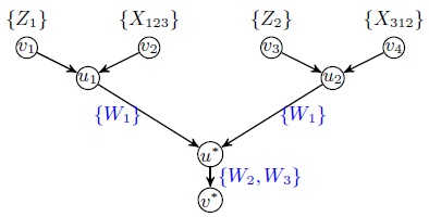
Thus, our lower bound works with judiciously chosen labels for the delivery phase signals and combines them with the cache signals in an appropriate way such that a given file is recovered a large number of times. It turns out that doing this systematically and tractably requires the development of several new ideas. For instance, the aforementioned chain of inequalities can be equivalently represented in terms of a directed tree with appropriate labels on its leaves and edges as shown in Fig. 3. In particular, the leaves of the tree are labeled with cache signals Z1Z_{1} and Z2Z_{2} and delivery phase signals X123X_{123} and X312X_{312}. Each internal node of the tree corresponds to the operation of combining the signals and its outgoing edge is labeled by the newly recovered file(s), e.g., at node u1u_{1}, the file W1W_{1} is recovered. Likewise at node u∗u^{*}, the files W2W_{2} and W3W_{3} are recovered. The lower bound can be obtained by summing the cardinalities of the edge labels. Towards the goal of generating these bounds in a systematic manner, we introduce the following definitions.

Definition 2

Directed in-tree. A directed graph 𝒯=(V,A)\mathcal{T}=(V,A), is called a directed in-tree if there is one designated node called the root such that from any other vertex v∈Vv\in V there is exactly one directed path from vv to the root.

The nodes in a directed in-tree that do not have any incoming edges are referred to as the leaves. The remaining nodes, excluding the leaves and the root are called internal nodes. Each node in a directed in-tree has at most one outgoing edge. We have the following definitions for a node v∈Vv\in V.

o​u​t​(v)\displaystyle out(v) ={u∈V:(v,u)∈A}, (outgoing neighbor) and,\displaystyle=\{u\in V:(v,u)\in A\},\text{~(outgoing neighbor) and},
i​n​(v)\displaystyle in(v) ={u∈V:(u,v)∈A}​ (incoming neighbor set).\displaystyle=\{u\in V:(u,v)\in A\}\text{~(incoming neighbor set).}
i​n−e​d​g​e​(v)\displaystyle in-edge(v) ={e∈A:e=(u,v)}​ (incoming edge set).\displaystyle=\{e\in A:e=(u,v)\}\text{~(incoming edge set)}.

In this work, we exclusively work with trees which are such that the in-degree of the root equals 1. There is a natural topological order in 𝒯\mathcal{T} whereby for nodes u∈𝒯u\in\mathcal{T} and v∈𝒯v\in\mathcal{T}, we say that u≻vu\succ v if there exists a sequence of edges that can be traversed to reach vv from uu. This sequence of edges is denoted p​a​t​h​(u,v)path(u,v).

Algorithm 1 Lower Bound Algorithm
1: 𝒯=(V,A)\mathcal{T}=(V,A) with leaves v1,…,vℓv_{1},\ldots,v_{\ell} and {l​a​b​e​l​(vi)}i=1ℓ\{label(v_{i})\}_{i=1}^{\ell}, such that 𝕎(vi)=∅,i=1,…,ℓ\mathds{W}(v_{i})=\emptyset,i=1,\dots,\ell.
2:
3: for i←1,…​ℓi\leftarrow 1,\dots\ell do
4:   Wn​e​w​(vi)=Δ⁡(vi,vi)W_{new}(v_{i})=\Delta(v_{i},v_{i}).
5:   x(vi,o​u​t​(vi))=Wn​e​w​(vi)x_{(v_{i},out(v_{i}))}=W_{new}(v_{i}).
6:   y(vi,o​u​t​(vi))=|Wn​e​w​(vi)|y_{(v_{i},out(v_{i}))}=|W_{new}(v_{i})|.
7: end for
8: while there exists an unlabeled edge do
9:   Pick an unlabeled node u∈Vu\in V such that all edges in i​n−e​d​g​e​(u)in-edge(u) are labeled.
10:   𝕎(u)=∪v∈i​n​(u)𝕎(v)∪Wn​e​w(v)\mathds{W}(u)=\cup_{v\in in(u)}\mathds{W}(v)\cup W_{new}(v).
11:   ℤ(u)=∪v∈i​n​(u)ℤ(v)\mathds{Z}(u)=\cup_{v\in in(u)}\mathds{Z}(v).
12:   𝔻(u)=∪v∈i​n​(u)𝔻(v)\mathds{D}(u)=\cup_{v\in in(u)}\mathds{D}(v).
13:   Wn​e​w​(u)=Δ⁡(u,u)∖𝕎⁡(u)W_{new}(u)=\Delta(u,u)\setminus\mathds{W}(u).
14:   x(u,o​u​t​(u))=Wn​e​w​(u)x_{(u,out(u))}=W_{new}(u).
15:   y(u,o​u​t​(u))=|Wn​e​w​(u)|y_{(u,out(u))}=|W_{new}(u)|.
16: end while
17: L=∑e∈AyeL=\sum_{e\in A}y_{e}.
Definition 3

Meeting point of nodes in a directed tree. Consider nodes v1v_{1} and v2v_{2} in a directed in-tree 𝒯=(V,A)\mathcal{T}=(V,A). We say that v1v_{1} and v2v_{2} meet at node uu if there exist p​a​t​h​(v1,u)path(v_{1},u) and p​a​t​h​(v2,u)path(v_{2},u) in 𝒯\mathcal{T} such that p​a​t​h​(v1,u)∩p​a​t​h​(v2,u)=∅path(v_{1},u)\cap path(v_{2},u)=\emptyset. As there exists a path from any node in 𝒯\mathcal{T} to the root node, it follows that the existence of node uu is guaranteed.

Let D=∪d1∈[N],…,dK∈[N]{Xd1,…,dK}D=\cup_{d_{1}\in[N],\dots,d_{K}\in[N]}\{X_{d_{1},\dots,d_{K}}\}.

Definition 4

Labeling of directed in-tree. Each node v∈𝒯v\in\mathcal{T} is assigned a label, denoted l​a​b​e​l​(v)label(v), which is a subset of {W1,…,WN}∪{Z1,…,ZK}∪D\{W_{1},\dots,W_{N}\}\cup\{Z_{1},\dots,Z_{K}\}\cup D. Moreover, we also specify 𝕎⁡(v)⊆{W1,…,WN}\mathds{W}(v)\subseteq\{W_{1},\dots,W_{N}\}, ℤ⁡(v)⊆{Z1,…,ZK}\mathds{Z}(v)\subseteq\{Z_{1},\dots,Z_{K}\} and 𝔻⁡(v)⊆D\mathds{D}(v)\subseteq D so that l​a​b​e​l​(v)=𝕎⁡(v)∪ℤ⁡(v)∪𝔻⁡(v)label(v)=\mathds{W}(v)\cup\mathds{Z}(v)\cup\mathds{D}(v).

In our formulation, the leaf nodes are denoted vi,i=1,…,ℓv_{i},i=1,\dots,\ell are such that 𝕎⁡(vi)=∅\mathds{W}(v_{i})=\emptyset.

Definition 5

We say that a singleton source subset {Wi}\{W_{i}\} is recoverable from the pair (Zj,Xd1,…,dK)(Z_{j},X_{d_{1},\dots,d_{K}}) if dj=id_{j}=i. Similarly, for a given set of caches Z′⊆{Z1,…,ZK}Z^{\prime}\subseteq\{Z_{1},\dots,Z_{K}\} and delivery phase signals D′⊆DD^{\prime}\subseteq D, we define a set R​e​c​(Z′,D′)⊆{W1,…,WN}Rec(Z^{\prime},D^{\prime})\subseteq\{W_{1},\dots,W_{N}\} to be the subset of the sources that can be recovered from pairs of the form (Zi,XJ)(Z_{i},X_{J}) where Zi∈Z′Z_{i}\in Z^{\prime} and JJ is a multiset of cardinality KK with entries from [N][N] such that XJ∈D′X_{J}\in D^{\prime}.

We let the entropy of a set of random variables equal the joint entropy of all the random variables in the set. We also let [x]+=max⁡(x,0)[x]^{+}=\max(x,0).

Given a directed tree 𝒯\mathcal{T} with appropriate labels on its leaves we present an algorithm that generates an inequality of the form α​R⋆+β​M≥L⁡(α,β)\alpha R^{\star}+\beta M\geq L(\alpha,\beta). For nodes u,v∈𝒯u,v\in\mathcal{T}, we define the following.

Δ⁡(u,v)\displaystyle\Delta(u,v) =R​e​c​(ℤ⁡(u),𝔻⁡(v)), and\displaystyle=Rec(\mathds{Z}(u),\mathds{D}(v)),\text{~and}
Wn​e​w​(u)\displaystyle W_{new}(u) =Δ⁡(u,u)∖𝕎⁡(u).\displaystyle=\Delta(u,u)\setminus\mathds{W}(u). (4)
Refer to caption
Fig. 3: Problem instance for Example 1. For clarity of presentation, only the Wn​e​w​(u)W_{new}(u) label has been shown on the edges.

Algorithm 1 operates as follows. It takes as input a directed in-tree 𝒯\mathcal{T} where each leaf vi,i=1,…,ℓv_{i},i=1,\dots,\ell has labels ℤ⁡(vi)\mathds{Z}(v_{i}) and 𝔻⁡(vi)\mathds{D}(v_{i}) (𝕎⁡(vi)\mathds{W}(v_{i}) is set to ∅\emptyset). The algorithm determines the files that are recovered at each viv_{i} and labels the corresponding outgoing edge with Wn​e​w​(vi)W_{new}(v_{i}) and |Wn​e​w​(vi)||W_{new}(v_{i})|. Following this, the algorithm propagates the labels further down the tree in the following manner. For a given node uu whose incoming edges are labeled, we set ℤ(u)=∪v∈i​n​(u)ℤ(v)\mathds{Z}(u)=\cup_{v\in in(u)}\mathds{Z}(v) and 𝔻(u)=∪v∈i​n​(u)𝔻(v)\mathds{D}(u)=\cup_{v\in in(u)}\mathds{D}(v), i.e., each of these labels is set to the union of the corresponding labels of the nodes that belong to the incoming node set of uu. Next, it sets 𝕎(u)=∪v∈i​n​(u)𝕎(v)∪Wn​e​w(v)\mathds{W}(u)=\cup_{v\in in(u)}\mathds{W}(v)\cup W_{new}(v), i.e., in addition to the 𝕎\mathds{W}-labels of the incoming node set, 𝕎⁡(u)\mathds{W}(u) also contains the new files that are recovered on the incident edges. Note that at each internal node certain cache signals and delivery phase signals meet, e.g., Z1Z_{1} and X123X_{123} meet at node u1u_{1} in Fig. 3. The outgoing edge of an internal node is labeled by the new files that are recovered at the node, e.g., at u1u_{1} the signals Z1Z_{1} and X123X_{123} recover the file W1W_{1}. We call a file new if it has not been recovered upstream of a given node. In a similar manner at u∗u^{*} one can recover all the files W1,…,W3W_{1},\dots,W_{3}; however only the set {W2,W3}\{W_{2},W_{3}\} is labeled on edge (u∗,v∗)(u^{*},v^{*}) as W1W_{1} was recovered upstream. This process is continued recursively, i.e., we label the outgoing edges with the new files that are recovered at node uu, propagate the labels and continue thereafter. The algorithm continues until it labels the last outgoing edge.

It can be seen that the operation of Algorithm 1 is in one to one correspondence with the new files recovered in the sequence of inequalities in the lower bound. For example, the outgoing labels of u1u_{1} and u2u_{2} in Fig. 3 correspond to step (a) in the inequalities in Example 1. We formalize this statement in the Appendix (Lemma 3) where we show that a valid lower bound is always obtained when applying Algorithm 1.

Definition 6

Problem Instance. Consider a given tree 𝒯\mathcal{T} with leaves vi,i=1,…,ℓv_{i},i=1,\dots,\ell that are labeled as discussed above. Let α=∑i=1ℓ|𝔻⁡(vi)|\alpha=\sum_{i=1}^{\ell}|\mathds{D}(v_{i})| and β=∑i=1ℓ|ℤ⁡(vi)|\beta=\sum_{i=1}^{\ell}|\mathds{Z}(v_{i})|. Suppose that the lower bound computed by Algorithm 1 equals LL. We define the associated problem instance as P⁡(𝒯,α,β,L,N,K)P(\mathcal{T},\alpha,\beta,L,N,K). We also define α^=|∪i=1ℓ𝔻(vi)|\hat{\alpha}=|\cup_{i=1}^{\ell}\mathds{D}(v_{i})| and β^=|∪i=1ℓℤ(vi)|\hat{\beta}=|\cup_{i=1}^{\ell}\mathds{Z}(v_{i})|. A problem instance P⁡(𝒯,α,β,L,N,K)P(\mathcal{T},\alpha,\beta,L,N,K) is said to be optimal if all instances of the form P′​(𝒯′,α,β,L′,N,K)P^{\prime}(\mathcal{T}^{\prime},\alpha,\beta,L^{\prime},N,K) are such that L′≤LL^{\prime}\leq L.

It is worth emphasizing that α^≤α\hat{\alpha}\leq\alpha and β^≤β\hat{\beta}\leq\beta as some cache and delivery phase signals may be repeated.

In the subsequent discussion, we focus on understanding the characteristics of optimal problem instances. Towards this end, we shall often start with a problem instance PP and modify it in appropriate ways to arrive at another instance P′P^{\prime}. For ease of presentation, when needed we shall refer to quantities in instance PP(P′P^{\prime}) by using the corresponding superscripts. For example for a node uu in PP (P′P^{\prime}), we will denote the set of new files by Wn​e​wP​(u)W_{new}^{P}(u) (Wn​e​wP′​(u)W_{new}^{P^{\prime}}(u)).

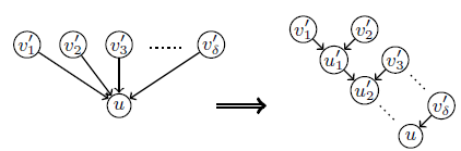
It is not too hard to see that it suffices to consider directed trees whose internal nodes have an in-degree at least two. In particular, if uu has in-degree equal to 11, it is evident that Wn​e​w​(u)=∅W_{new}(u)=\emptyset and thus, |Wn​e​w​(u)|=0|W_{new}(u)|=0. In addition, we claim that w.l.o.g. it suffices to consider trees where internal nodes have in-degree at most two. Therefore, we will assume that all internal nodes have degree equal to two. More specifically, we can show the following property of problem instances (the proof appears in the Appendix).

Claim 1

Consider a problem instance P⁡(𝒯,α,β,L,N,K)P(\mathcal{T},\alpha,\beta,L,N,K) such that there exists a node u∈𝒯u\in\mathcal{T} with |i​n​(u)|≥3|in(u)|\geq 3. Then, there exists another instance P′​(𝒯′,α,β,L′,N,K)P^{\prime}(\mathcal{T}^{\prime},\alpha,\beta,L^{\prime},N,K) where L′≥LL^{\prime}\geq L and |i​n​(u)|≤2|in(u)|\leq 2 for all nodes u∈𝒯′u\in\mathcal{T}^{\prime}.

Henceforth, we assume that all internal nodes in the problem instances under consideration have in-degree equal to two. Claim 1 can also be used to conclude that each leaf vv in an instance PP is such that either |ℤ⁡(v)|=1|\mathds{Z}(v)|=1 or |𝔻⁡(v)|=1|\mathds{D}(v)|=1 but not both. Indeed, if there exists a leaf vv that violates this condition, we can use the modification in the proof of Claim 1 to replace vv by a directed in-tree so that the condition is satisfied. If |ℤ⁡(v)|=1|\mathds{Z}(v)|=1, we call vv a cache node; if |𝔻⁡(v)|=1|\mathds{D}(v)|=1 we call it a delivery phase node. In the subsequent discussion we will assume that the delivery phase nodes are labeled in an arbitrary order v1,…,vαv_{1},\dots,v_{\alpha} and the cache nodes from vα+1,…,vα+βv_{\alpha+1},\dots,v_{\alpha+\beta}, where we note that α+β=ℓ\alpha+\beta=\ell. Moreover, we let 𝒟={v1,…,vα}\mathcal{D}=\{v_{1},\dots,v_{\alpha}\} and 𝒞={vα+1,…,vα+β}\mathcal{C}=\{v_{\alpha+1},\dots,v_{\alpha+\beta}\}.

Refer to caption
Fig. 4: For a given node u∈𝒯u\in\mathcal{T}, its in-neighbors are denoted ulu_{l} and uru_{r}. The corresponding subtrees are denoted 𝒯u⁡(l)\mathcal{T}_{u(l)} and 𝒯u⁡(r)\mathcal{T}_{u(r)} and are shown enclosed in the dotted boxes.

In the tree 𝒯\mathcal{T} corresponding to problem instance P⁡(𝒯,α,β,L,N,K)P(\mathcal{T},\alpha,\beta,L,N,K), consider an internal node uu and the edge e=(u,v)e=(u,v). In the subsequent discussion, we shall use 𝒯u\mathcal{T}_{u} to refer to the subtree that has its last edge as (u,o​u​t​(u))(u,out(u)), i.e., the subtree that is rooted at o​u​t​(u)out(u). The incoming edges into uu, denoted (ul,u)(u_{l},u) and (ur,u)(u_{r},u) are the last edges of the disjoint left and right subtrees denoted 𝒯u⁡(l)\mathcal{T}_{u(l)} and 𝒯u⁡(r)\mathcal{T}_{u(r)} respectively (see Fig. 4). Each of these subtrees defines a problem instance Pl=P⁡(𝒯u⁡(l),αl,βl,Ll,N,K)P_{l}=P(\mathcal{T}_{u(l)},\alpha_{l},\beta_{l},L_{l},N,K) and Pr=P⁡(𝒯u⁡(r),αr,βr,Lr,N,K)P_{r}=P(\mathcal{T}_{u(r)},\alpha_{r},\beta_{r},L_{r},N,K). We denote the set of delivery phase nodes and cache nodes in 𝒯u⁡(r)\mathcal{T}_{u(r)} by

𝒟u⁡(r)\displaystyle\mathcal{D}_{u(r)} ={v∈𝒟:v∈𝒯u⁡(r)}​ and\displaystyle=\{v\in\mathcal{D}:v\in\mathcal{T}_{u(r)}\}\text{~and}
𝒞u⁡(r)\displaystyle\mathcal{C}_{u(r)} ={v∈𝒞:v∈𝒯u⁡(r)},\displaystyle=\{v\in\mathcal{C}:v\in\mathcal{T}_{u(r)}\},

with similar definitions for 𝒟u⁡(l)\mathcal{D}_{u(l)} and 𝒞u⁡(l)\mathcal{C}_{u(l)}. We also let

𝒟u\displaystyle\mathcal{D}_{u} =𝒟u⁡(l)∪𝒟u⁡(r), and\displaystyle=\mathcal{D}_{u(l)}\cup\mathcal{D}_{u(r)},\text{~and}
𝒞u\displaystyle\mathcal{C}_{u} =𝒞u⁡(l)∪𝒞u⁡(r).\displaystyle=\mathcal{C}_{u(l)}\cup\mathcal{C}_{u(r)}.

Let Γl=∪v∈𝒯u⁡(l)Wn​e​w(v)\Gamma_{l}=\cup_{v\in\mathcal{T}_{u(l)}}W_{new}(v) and Γr=∪v∈𝒯u⁡(r)Wn​e​w(v)\Gamma_{r}=\cup_{v\in\mathcal{T}_{u(r)}}W_{new}(v), i.e., Γl\Gamma_{l} and Γr\Gamma_{r} are the subsets of {W1,…,WN}\{W_{1},\dots,W_{N}\} that are used up in the problem instances PlP_{l} and PrP_{r} respectively. It can be observed that Γl=Δ⁡(ul,ul)\Gamma_{l}=\Delta(u_{l},u_{l}) and Γr=Δ⁡(ur,ur)\Gamma_{r}=\Delta(u_{r},u_{r}).

We shall often need to reason about the files recovered at the node uu from the different subtrees. For instance, the set of cache nodes in 𝒯u⁡(r)\mathcal{T}_{u(r)} and the delivery phase signals in 𝒯u⁡(l)\mathcal{T}_{u(l)} meet and recover a subset of the files at uu. This set of files corresponds to those recovered from ℤ⁡(ur)∖ℤ⁡(ul)\mathds{Z}(u_{r})\setminus\mathds{Z}(u_{l}) and 𝔻⁡(ul)\mathds{D}(u_{l}), and can be informally thought of as the files recovered when going from right to left. Accordingly, we have the following definitions.

Δr​l​(u)\displaystyle\Delta_{rl}(u) =R​e​c​(ℤ⁡(ur)∖ℤ⁡(ul),𝔻⁡(ul)), and\displaystyle=Rec(\mathds{Z}(u_{r})\setminus\mathds{Z}(u_{l}),\mathds{D}(u_{l})),\text{~and}
Δl​r​(u)\displaystyle\Delta_{lr}(u) =R​e​c​(ℤ⁡(ul)∖ℤ⁡(ur),𝔻⁡(ur)).\displaystyle=Rec(\mathds{Z}(u_{l})\setminus\mathds{Z}(u_{r}),\mathds{D}(u_{r})).

Note that by definition, we have

Δ⁡(u,u)\displaystyle\Delta(u,u) =R​e​c​(ℤ⁡(u),𝔻⁡(u))\displaystyle=Rec(\mathds{Z}(u),\mathds{D}(u))
=R​e​c​(ℤ⁡(ul)∪ℤ⁡(ur),𝔻⁡(ul)∪𝔻⁡(ur))\displaystyle=Rec(\mathds{Z}(u_{l})\cup\mathds{Z}(u_{r}),\mathds{D}(u_{l})\cup\mathds{D}(u_{r}))
=R​e​c​(ℤ⁡(ul),𝔻⁡(ul))∪R​e​c​(ℤ⁡(ur),𝔻⁡(ur))∪R​e​c​(ℤ⁡(ul),𝔻⁡(ur))∪R​e​c​(ℤ⁡(ur),𝔻⁡(ul))\displaystyle=Rec(\mathds{Z}(u_{l}),\mathds{D}(u_{l}))\cup Rec(\mathds{Z}(u_{r}),\mathds{D}(u_{r}))\cup Rec(\mathds{Z}(u_{l}),\mathds{D}(u_{r}))\cup Rec(\mathds{Z}(u_{r}),\mathds{D}(u_{l}))
=(a)R​e​c​(ℤ⁡(ul),𝔻⁡(ul))∪R​e​c​(ℤ⁡(ur),𝔻⁡(ur))∪R​e​c​(ℤ⁡(ul)∖ℤ⁡(ur),𝔻⁡(ur))∪R​e​c​(ℤ⁡(ur)∖ℤ⁡(ul),𝔻⁡(ul))\displaystyle\stackrel{{\scriptstyle(a)}}{{=}}Rec(\mathds{Z}(u_{l}),\mathds{D}(u_{l}))\cup Rec(\mathds{Z}(u_{r}),\mathds{D}(u_{r}))\cup Rec(\mathds{Z}(u_{l})\setminus\mathds{Z}(u_{r}),\mathds{D}(u_{r}))\cup Rec(\mathds{Z}(u_{r})\setminus\mathds{Z}(u_{l}),\mathds{D}(u_{l}))
=Δ⁡(ℤ⁡(ul),𝔻⁡(ul))⏟from 𝒯u⁡(l)∪Δ⁡(ℤ⁡(ur),𝔻⁡(ur))⏟from 𝒯u⁡(r)∪Δl​r​(u)∪Δr​l​(u), and\displaystyle=\underbrace{\Delta(\mathds{Z}(u_{l}),\mathds{D}(u_{l}))}_{\text{from $\mathcal{T}_{u(l)}$}}\cup\underbrace{\Delta(\mathds{Z}(u_{r}),\mathds{D}(u_{r}))}_{\text{from $\mathcal{T}_{u(r)}$}}\cup\Delta_{lr}(u)\cup\Delta_{rl}(u),\text{~and}
𝕎⁡(u)\displaystyle\mathds{W}(u) =Δ⁡(ℤ⁡(ul),𝔻⁡(ul))∪Δ⁡(ℤ⁡(ur),𝔻⁡(ur)),\displaystyle=\Delta(\mathds{Z}(u_{l}),\mathds{D}(u_{l}))\cup\Delta(\mathds{Z}(u_{r}),\mathds{D}(u_{r})),

where (a)(a) follows since the R​e​c​(ℤ⁡(ul),𝔻⁡(ur))Rec(\mathds{Z}(u_{l}),\mathds{D}(u_{r})) potentially contains some files that have already been recovered in R​e​c​(ℤ⁡(ur),𝔻⁡(ur))Rec(\mathds{Z}(u_{r}),\mathds{D}(u_{r})). The other equality holds because of similar reasoning. Therefore, it follows that

Wn​e​w​(u)\displaystyle W_{new}(u) =Δ⁡(u,u)∖𝕎⁡(u)\displaystyle=\Delta(u,u)\setminus\mathds{W}(u)
=Δr​l​(u)∪Δl​r​(u)∖𝕎⁡(u).\displaystyle=\Delta_{rl}(u)\cup\Delta_{lr}(u)\setminus\mathds{W}(u). (5)

Note that based on Algorithm 1, we can conclude that

𝕎⁡(u)\displaystyle\mathds{W}(u) =∪v∈{ur,ul}𝕎(v)∪Wn​e​w(v)\displaystyle=\cup_{v\in\{u_{r},u_{l}\}}\mathds{W}(v)\cup W_{new}(v)
=∪v≻uWn​e​w(v) (by arguing inductively).\displaystyle=\cup_{v\succ u}W_{new}(v)\text{~(by arguing inductively)}. (6)
Algorithm 2 Computing ψ\psi
1: P⁡(𝒯,α,β,L,N,K)P(\mathcal{T},\alpha,\beta,L,N,K), Array Ω⁡(u,δu)\Omega(u,\delta_{u}), where u∈𝒯u\in\mathcal{T}, δu⊆Wn​e​w​(u),|δu|=1\delta_{u}\subseteq W_{new}(u),|\delta_{u}|=1.
2: Initialization
3:   for all u∈𝒯u\in\mathcal{T}, δu⊆Wn​e​w​(u)\delta_{u}\subseteq W_{new}(u) where |δu|=1|\delta_{u}|=1 do
4:    Ω⁡(u,δu)←0\Omega(u,\delta_{u})\leftarrow 0,
5:   end for
6: end Initialization
7: for i←1i\leftarrow 1 to α\alpha do
8:   for all v′∈𝒞v^{\prime}\in\mathcal{C} do
9:    Let uu be the meeting point of viv_{i} and v′v^{\prime}.
10:    δu=Δ⁡(v′,vi)\delta_{u}=\Delta(v^{\prime},v_{i}).
11:    if δu∈Wn​e​w​(u)\delta_{u}\in W_{new}(u) and Ω⁡(u,δu)==0\Omega(u,\delta_{u})==0 then
12:      ψ⁡(vi,v′)←1\psi(v_{i},v^{\prime})\leftarrow 1, and Ω⁡(u,δu)←1\Omega(u,\delta_{u})\leftarrow 1.
13:    else
14:      ψ⁡(vi,v′)←0\psi(v_{i},v^{\prime})\leftarrow 0.
15:    end if
16:   end for
17: end for

For the subsequent discussion, it will be useful to express the value of the lower bound LL for an instance P⁡(𝒯,α,β,L,N,K)P(\mathcal{T},\alpha,\beta,L,N,K) in a functional form. In particular, we define the function ψ:𝒟×𝒞→{0,1}\psi:\mathcal{D}\times\mathcal{C}\rightarrow\{0,1\} that allows us to express LL in another way. For nodes vi∈𝒟,v′∈𝒞v_{i}\in\mathcal{D},v^{\prime}\in\mathcal{C} we can define their meeting point u∈𝒯u\in\mathcal{T}. The function ψ⁡(vi,v′)\psi(v_{i},v^{\prime}) is determined by means of Algorithm 2, where the sequence in which we pick the nodes v1,…,vαv_{1},\dots,v_{\alpha} is fixed. Each element of Wn​e​w​(u)W_{new}(u) can be recovered from multiple pairs of nodes that meet there. The array Ω⁡(u,δu)\Omega(u,\delta_{u}) keeps track of the first time the file δu\delta_{u} is encountered. The function ψ⁡(vi,v′)\psi(v_{i},v^{\prime}) takes the value 11 if the file W∗W^{*} recovered from the pair (ℤ⁡(v′),𝔻⁡(vi))(\mathds{Z}(v^{\prime}),\mathds{D}(v_{i})) at uu belongs to Wn​e​w​(u)W_{new}(u) and has not been encountered before and 0 otherwise. A formal description is given in Algorithm 2.

Claim 2

For an instance P⁡(𝒯,α,β,L,N,K)P(\mathcal{T},\alpha,\beta,L,N,K) the following equality holds

L=∑i=1α∑v′∈𝒞ψ⁡(vi,v′).\displaystyle L=\sum_{i=1}^{\alpha}\sum_{v^{\prime}\in\mathcal{C}}\psi(v_{i},v^{\prime}). (7)

Proof:  We first note that at the end of Algorithm 2, we have Ω⁡(u,δu)=1\Omega(u,\delta_{u})=1 for all u∈𝒯u\in\mathcal{T} and all δu⊆Wn​e​w​(u)\delta_{u}\subseteq W_{new}(u) such that |δu|=1|\delta_{u}|=1. To see this suppose that there is a u1∈𝒯u_{1}\in\mathcal{T} and a singleton subset δu1\delta_{u_{1}} of Wn​e​w​(u1)W_{new}(u_{1}) such that Ω⁡(u1,δu1)=0\Omega(u_{1},\delta_{u_{1}})=0. Now δu1\delta_{u_{1}} is recovered from some delivery phase node and cache node, otherwise it would not be a subset of Wn​e​w​(u1)W_{new}(u_{1}). As our algorithm considers all pairs of delivery phase nodes and cache nodes, at the end of the algorithm it has to be the case that Ω⁡(u1,δu1)=1\Omega(u_{1},\delta_{u_{1}})=1.

Next, we note that for each pair (u1,δu1)(u_{1},\delta_{u_{1}}) where u1∈𝒯u_{1}\in\mathcal{T} and δu1\delta_{u_{1}} is singleton subset of Wn​e​w​(u1)W_{new}(u_{1}), we can identify a unique pair of nodes (vi,v′)(v_{i},v^{\prime}) where vi∈𝒟v_{i}\in\mathcal{D} and v′∈𝒞v^{\prime}\in\mathcal{C} such that ψ⁡(vi,v′)\psi(v_{i},v^{\prime}) and Ω⁡(u1,δu1)\Omega(u_{1},\delta_{u_{1}}) are set to 1 at the same step of the algorithm. The remaining pairs (vi,v′)(v_{i},v^{\prime}) that cannot be put in one to one correspondence with a pair (u1,δu1)(u_{1},\delta_{u_{1}}) are such that ψ⁡(vi,v′)\psi(v_{i},v^{\prime}) are set to 0. Moreover as ∑u∈𝒯∑δu⊆Wn​e​w​(u),|δu|=1Ω⁡(u,δu)=∑u∈𝒯|Wn​e​w​(u)|=L\sum_{u\in\mathcal{T}}\sum_{\delta_{u}\subseteq W_{new}(u),|\delta_{u}|=1}\Omega(u,\delta_{u})=\sum_{u\in\mathcal{T}}|W_{new}(u)|=L, it follows that L=∑i=1α∑v′∈𝒞ψ⁡(vi,v′)L=\sum_{i=1}^{\alpha}\sum_{v^{\prime}\in\mathcal{C}}\psi(v_{i},v^{\prime}).

Refer to caption
Fig. 5: Problem instance of Example 2. There are three users and the server contains four files.

We now illustrate the definitions introduced above by means of the following example.

Example 2

The problem instance in Fig. 5 has seven internal nodes, {u1,…,u6,u∗}\{u_{1},\ldots,u_{6},u^{*}\}. In the initialization step, Algorithm 2 sets Ω⁡(ui,{W1})=0\Omega(u_{i},\{W_{1}\})=0 for 1≤i≤41\leq i\leq 4, Ω⁡(ui,{W2})=Ω⁡(ui,{W3})=0\Omega(u_{i},\{W_{2}\})=\Omega(u_{i},\{W_{3}\})=0 for i=5,6i=5,6 and Ω⁡(u∗,{W4})=0\Omega(u^{*},\{W_{4}\})=0. In the next step, for node v1v_{1} it sets ψ⁡(v1,v5)=1\psi(v_{1},v_{5})=1, Ω⁡(u1,{W1})=1\Omega(u_{1},\{W_{1}\})=1 (for v5∈𝒞v_{5}\in\mathcal{C}) and ψ⁡(v1,v6)=1\psi(v_{1},v_{6})=1, Ω⁡(u5,{W2})=1\Omega(u_{5},\{W_{2}\})=1 (for v6∈𝒞v_{6}\in\mathcal{C}). For v7∈𝒞v_{7}\in\mathcal{C} we have δu∗=Δ⁡(v7,v1)={W3}\delta_{u^{*}}=\Delta(v_{7},v_{1})=\{W_{3}\} and since W3∉Wn​e​w​(u∗)={W4}W_{3}\notin W_{new}(u^{*})=\{W_{4}\} therefore ψ⁡(v1,v7)=0\psi(v_{1},v_{7})=0. By the same argument we have ψ⁡(v1,v8)=0\psi(v_{1},v_{8})=0. Thus, the contribution of v1v_{1} to the lower bound, namely ∑v′∈𝒞ψ⁡(v1,v′)=2\sum_{v^{\prime}\in\mathcal{C}}\psi(v_{1},v^{\prime})=2. The complete description of the steps after the initialization, is shown in Table I. The table should be read in column order from left to right. Within a column, the order of the operations is from top to bottom. Note that there are two cases, v3∈𝒟,v6∈𝒞v_{3}\in\mathcal{D},v_{6}\in\mathcal{C} and v4∈𝒟,v6∈𝒞v_{4}\in\mathcal{D},v_{6}\in\mathcal{C} where ψ⁡(⋅,⋅)\psi(\cdot,\cdot) value is set to 00 (since the corresponding Ω⁡(⋅,⋅)\Omega(\cdot,\cdot) values are already 11). In both cases δu∗={W4}\delta_{u^{*}}=\{W_{4}\} and since W4W_{4} is recovered already, Ω⁡(u∗,{W4})\Omega(u^{*},\{W_{4}\}) has already been set to 11 when considering v2∈𝒟,v7∈𝒞v_{2}\in\mathcal{D},v_{7}\in\mathcal{C}. Therefore ψ⁡(v4,v6)=ψ⁡(v3,v6)=0\psi(v_{4},v_{6})=\psi(v_{3},v_{6})=0. Another point to be noted is that delivery phase node v2v_{2} contributes three files towards LL while the other delivery nodes contribute only two files each.

setting v1v_{1} v2v_{2} v3v_{3} v4v_{4}
v5v_{5} δu1=W1\delta_{u_{1}}=W_{1} δu5=W3\delta_{u_{5}}=W_{3} δu∗=W2\delta_{u^{*}}=W_{2} δu∗=W1\delta_{u^{*}}=W_{1}
ψ⁡(v1,v5)=1\psi(v_{1},v_{5})=1 ψ⁡(v2,v5)=1\psi(v_{2},v_{5})=1 ψ⁡(v3,v5)=0\psi(v_{3},v_{5})=0 ψ⁡(v4,v5)=0\psi(v_{4},v_{5})=0
Ω⁡(u1,W1)=1\Omega(u_{1},W_{1})=1 Ω⁡(u5,W3)=1\Omega(u_{5},W_{3})=1
v6v_{6} δu5=W2\delta_{u_{5}}=W_{2} δu2=W1\delta_{u_{2}}=W_{1} δu∗=W4\delta_{u^{*}}=W_{4} δu∗=W4\delta_{u^{*}}=W_{4}
ψ⁡(v1,v6)=1\psi(v_{1},v_{6})=1 ψ⁡(v2,v6)=1\psi(v_{2},v_{6})=1 ψ⁡(v3,v6)=0\psi(v_{3},v_{6})=0 ψ⁡(v4,v6)=0\psi(v_{4},v_{6})=0
Ω⁡(u5,W2)=1\Omega(u_{5},W_{2})=1 Ω⁡(u2,W1)=1\Omega(u_{2},W_{1})=1 Ω⁡(u∗,W4)=1\Omega(u^{*},W_{4})=1 Ω⁡(u∗,W4)=1\Omega(u^{*},W_{4})=1
v7v_{7} δu∗=W3\delta_{u^{*}}=W_{3} δu∗=W4\delta_{u^{*}}=W_{4} δu3=W1\delta_{u_{3}}=W_{1} δu6=W2\delta_{u_{6}}=W_{2}
ψ⁡(v1,v7)=0\psi(v_{1},v_{7})=0 ψ⁡(v2,v7)=1\psi(v_{2},v_{7})=1 ψ⁡(v3,v7)=1\psi(v_{3},v_{7})=1 ψ⁡(v4,v7)=1\psi(v_{4},v_{7})=1
Ω⁡(u∗,W4)=1\Omega(u^{*},W_{4})=1 Ω⁡(u3,W1)=1\Omega(u_{3},W_{1})=1 Ω⁡(u6,W2)=1\Omega(u_{6},W_{2})=1
v8v_{8} δu∗=W1\delta_{u^{*}}=W_{1} δu∗=W3\delta_{u^{*}}=W_{3} δu6=W2\delta_{u_{6}}=W_{2} δu4=W3\delta_{u_{4}}=W_{3}
ψ⁡(v1,v8)=0\psi(v_{1},v_{8})=0 ψ⁡(v2,v8)=0\psi(v_{2},v_{8})=0 ψ⁡(v3,v8)=1\psi(v_{3},v_{8})=1 ψ⁡(v4,v8)=1\psi(v_{4},v_{8})=1
Ω⁡(u6,W2)=1\Omega(u_{6},W_{2})=1 Ω⁡(u4,W3)=1\Omega(u_{4},W_{3})=1
TABLE I: The steps in Algorithm 2 after initialization when applied to Example 2. The steps flow from the leftmost to the rightmost column, and in each column from the top to the bottom row.
Corollary 1

For an instance P⁡(𝒯,α,β,L,N,K)P(\mathcal{T},\alpha,\beta,L,N,K), we have L≤α​min⁡(β,K)L\leq\alpha\min(\beta,K). Moreover, if N≥α​min⁡(β,K)N\geq\alpha\min(\beta,K), then there exists an instance such that L=α​min⁡(β,K)L=\alpha\min(\beta,K).

Proof:  For a node viv_{i}, where 1≤i≤α1\leq i\leq\alpha, we have

∑v′∈𝒞ψ⁡(vi,v′)\displaystyle\sum_{v^{\prime}\in\mathcal{C}}\psi(v_{i},v^{\prime}) ≤|∪v′∈𝒞ℤ(v′)|\displaystyle\leq|\cup_{v^{\prime}\in\mathcal{C}}\mathds{Z}(v^{\prime})|
=β^,\displaystyle=\hat{\beta},
≤min⁡(β,K).\displaystyle\leq\min(\beta,K). (8)

Let uu denote the meeting point of v′v^{\prime} and viv_{i}. The first inequality above holds since ψ⁡(vi,v′)=1\psi(v_{i},v^{\prime})=1 implies that δu=Δ⁡(v′,vi)⊆Wn​e​w​(u)\delta_{u}=\Delta(v^{\prime},v_{i})\subseteq W_{new}(u) and

∑v′∈𝒞ψ(vi,v′)≤|∪v′∈𝒞Rec(𝔻(vi),ℤ(v′))|=|Rec(𝔻(vi),∪v′∈𝒞ℤ(v′))|≤|∪v′∈𝒞ℤ(v′)|.\sum_{v^{\prime}\in\mathcal{C}}\psi(v_{i},v^{\prime})\leq|\cup_{v^{\prime}\in\mathcal{C}}Rec(\mathds{D}(v_{i}),\mathds{Z}(v^{\prime}))|=|Rec(\mathds{D}(v_{i}),\cup_{v^{\prime}\in\mathcal{C}}\mathds{Z}(v^{\prime}))|\leq|\cup_{v^{\prime}\in\mathcal{C}}\mathds{Z}(v^{\prime})|.

From eq. (8) we can conclude that L=∑i=1α∑v′∈𝒞ψ⁡(vi,v′)≤α​min⁡(β,K)L=\sum_{i=1}^{\alpha}\sum_{v^{\prime}\in\mathcal{C}}\psi(v_{i},v^{\prime})\leq\alpha\min(\beta,K). If N≥α​min⁡(β,K)N\geq\alpha\min(\beta,K), it is easy to construct an instance with L=α​min⁡(β,K)L=\alpha\min(\beta,K). We simply pick any directed tree on α+β\alpha+\beta leaves. Let the cache node indices be Z1Z_{1} repeated β−min⁡(β,K)+1\beta-\min(\beta,K)+1 times and Z2,Z3,…,Zmin⁡(β,K)−1,Zmin⁡(β,K)Z_{2},Z_{3},\dots,Z_{\min(\beta,K)-1},Z_{\min(\beta,K)}. Suppose that node v∈𝒟,v′∈𝒞′v\in\mathcal{D},v^{\prime}\in\mathcal{C}^{\prime} meet at node uu. We label the delivery phase leaves such that |∪(v,v′)∈𝒟×𝒞′Δ(v′,v)|=αmin(β,K)|\cup_{(v,v^{\prime})\in\mathcal{D}\times\mathcal{C}^{\prime}}\Delta(v^{\prime},v)|=\alpha\min(\beta,K). This can be done since NN is large enough so that we can choose the labels such that R​e​c​(ℤ⁡(v1′),𝔻⁡(v1))∩R​e​c​(ℤ⁡(v2′),𝔻⁡(v2))=∅Rec(\mathds{Z}(v_{1}^{\prime}),\mathds{D}(v_{1}))\cap Rec(\mathds{Z}(v_{2}^{\prime}),\mathds{D}(v_{2}))=\emptyset for v1′,v2′∈𝒞′v_{1}^{\prime},v_{2}^{\prime}\in\mathcal{C}^{\prime} and v1,v2∈𝒟v_{1},v_{2}\in\mathcal{D}. For instance, initialize 𝔻⁡(v)=X1,1,…,1\mathds{D}(v)=X_{1,1,\ldots,1} for all v∈𝒟v\in\mathcal{D} and then set 𝔻⁡(vi)=Xd1,…,dK\mathds{D}(v_{i})=X_{d_{1},\ldots,d_{K}}, dj=(i−1)​α+jd_{j}=(i-1)\alpha+j for j=1,…,min⁡(β,K)j=1,\ldots,\min(\beta,K), and i=1,…,αi=1,\ldots,\alpha. We illustrate the construction outlined above by means of the following example.

Example 3

Let α=β=2\alpha=\beta=2, K=2K=2, and N=4N=4. We arbitrary pick a directed tree with v1,v2v_{1},v_{2} as delivery nodes and v3,v4v_{3},v_{4} as cache nodes. We label ℤ⁡(v3)=Z1\mathds{Z}(v_{3})=Z_{1} and ℤ⁡(v3)=Z2\mathds{Z}(v_{3})=Z_{2}, and delivery nodes as 𝔻⁡(v1)=X1,2\mathds{D}(v_{1})=X_{1,2} and 𝔻⁡(v2)=X3,4\mathds{D}(v_{2})=X_{3,4}. Such a problem instance is illustrated in Fig. 6 (a)(a). As we will see later, this instance is not efficient in reusing files.

At this point we have established that for a given problem instance P⁡(𝒯,α,β,L,N,K)P(\mathcal{T},\alpha,\beta,L,N,K), we can always generate an inequality of the form α​R⋆+β​M≥L\alpha R^{\star}+\beta M\geq L. It is natural to therefore consider the optimal problem instances that maximize the lower bound for a given value of α,β,N\alpha,\beta,N and KK.

Definition 7

For given α,β,N\alpha,\beta,N and KK, we say that a problem instance P⁡(𝒯∗,α,β,L∗,N,K)P(\mathcal{T}^{*},\alpha,\beta,L^{*},N,K) is optimal if all problem instances 𝑂𝑃𝐸𝑁P′​(𝒯,α,β,L,N,K))P^{\prime}(\mathcal{T},\alpha,\beta,L,N,K)) are such that L∗≥LL^{*}\geq L.

Recall that β^=|∪i=1ℓℤ(vi)|\hat{\beta}=|\cup_{i=1}^{\ell}\mathds{Z}(v_{i})|. For a problem instance P⁡(𝒯,α,β,L,N,K)P(\mathcal{T},\alpha,\beta,L,N,K), it may be possible that β^<min⁡(β,K)\hat{\beta}<\min(\beta,K). However, given such an instance, we can convert it into another instance where β^=min⁡(β,K)\hat{\beta}=\min(\beta,K) without reducing the value of LL. In fact the following stronger statement holds (see Appendix -B for a proof).

Claim 3

For a problem instance P⁡(𝒯,α,β,L,N,K)P(\mathcal{T},\alpha,\beta,L,N,K) suppose that there exists an internal node u∗u^{*} with associated problem instance P∗=P⁡(𝒯u∗,α∗,β∗,L∗,N∗,K)P^{*}=P(\mathcal{T}_{u^{*}},\alpha^{*},\beta^{*},L^{*},N^{*},K) such that the following condition holds.

β^∗<min⁡(β∗,K).\hat{\beta}^{*}<\min(\beta^{*},K).

Then, there exists another problem instance P′​(𝒯′,α,β,L′,N,K)P^{\prime}(\mathcal{T}^{\prime},\alpha,\beta,L^{\prime},N,K) where L′≥LL^{\prime}\geq L such that the above condition does not hold.

The next claim formalizes the intuitive fact that permuting the cache nodes and the delivery phase signals by the same permutation does not change the 𝕎\mathds{W} labels and the lower bound of the instance.

Claim 4

Let P⁡(𝒯,α,β,L,N,K)P(\mathcal{T},\alpha,\beta,L,N,K) to be a problem instance and let π:[K]⟶[K]\pi:[K]\longrightarrow[K] to be a bijective mapping with inverse σ\sigma. Assume that the problem instance P′​(𝒯′,α,β,L′,N,K)P^{\prime}(\mathcal{T}^{\prime},\alpha,\beta,L^{\prime},N,K) is obtained from PP under the following changes for all v∈𝒟v\in\mathcal{D} and v′∈𝒞v^{\prime}\in\mathcal{C},

  • •

    assume ℤP​(v)=Zi\mathds{Z}^{P}(v)=Z_{i}, then set ℤP′​(v)=Zπ⁡(i)\mathds{Z}^{P^{\prime}}(v)=Z_{\pi(i)},

  • •

    assume 𝔻P​(v)=Xd1,…,dK\mathds{D}^{P}(v)=X_{d_{1},\ldots,d_{K}}, then set 𝔻P′​(v)=Xdσ⁡(1),…,dσ⁡(K)\mathds{D}^{P^{\prime}}(v)=X_{d_{\sigma(1)},\ldots,d_{\sigma(K)}},

then Wn​e​wP′​(u)=Wn​e​wP​(u)W_{new}^{P^{\prime}}(u)=W_{new}^{P}(u), 𝕎P′​(u)=𝕎P​(u)\mathds{W}^{P^{\prime}}(u)=\mathds{W}^{P}(u) for u∈𝒯u\in\mathcal{T}, and L′=LL^{\prime}=L.

Proof:  We note that

R​e​c​(Zi,Xd1,…,dK)=Wdi=Wdσ⁡(π⁡(i))=R​e​c​(Zπ⁡(i),Xdσ⁡(1),…,dσ⁡(K))Rec(Z_{i},X_{d_{1},\ldots,d_{K}})=W_{d_{i}}=W_{d_{\sigma(\pi(i))}}=Rec(Z_{\pi(i)},X_{d_{\sigma(1)},\ldots,d_{\sigma(K)}})

for i=1,…,Ki=1,\ldots,K. Therefore, for any v∈𝒟v\in\mathcal{D} and v′∈𝒞v^{\prime}\in\mathcal{C}, we have ΔP′​(v′,v)=ΔP​(v′,v)\Delta^{P^{\prime}}(v^{\prime},v)=\Delta^{P}(v^{\prime},v) and more generally ΔP′​(u,u)=ΔP​(u,u)\Delta^{P^{\prime}}(u,u)=\Delta^{P}(u,u). From this and that 𝕎P​(u)=ΔP​(ul,ul)∪ΔP​(ur,ur)\mathds{W}^{P}(u)=\Delta^{P}(u_{l},u_{l})\cup\Delta^{P}(u_{r},u_{r}), we have 𝕎P​(u)=𝕎P′​(u)\mathds{W}^{P}(u)=\mathds{W}^{P^{\prime}}(u) for any u∈𝒯u\in\mathcal{T}. Using eq. (4), we have Wn​e​wP′​(u)=Wn​e​wP​(u)W^{P^{\prime}}_{new}(u)=W^{P}_{new}(u) for all u∈𝒯′u\in\mathcal{T}^{\prime}. Consequently, it follows that L′=LL^{\prime}=L.

Henceforth, we will assume w.l.o.g. that β^=min⁡(β,K)\hat{\beta}=\min(\beta,K) and that Claim 3 holds. Our next lemma shows a structural property of problem instances. Namely for an instance where L<α​min⁡(β,K)L<\alpha\min(\beta,K), increasing the number of files allows us to increase the value of LL. This lemma is a key ingredient in our proof of the main theorem (the proof appears in the Appendix).

Lemma 1

Let P=P⁡(𝒯,α,β,L,K,N)P=P(\mathcal{T},\alpha,\beta,L,K,N) be an instance where L<α​min⁡(β,K)L<\alpha\min(\beta,K). Then, we can construct a new instance P′=P⁡(𝒯′,α,β,L′,K,N+1)P^{\prime}=P(\mathcal{T}^{\prime},\alpha,\beta,L^{\prime},K,N+1), where L′=L+1L^{\prime}=L+1.

Informally, another property of optimal problem instances is that the same file is recovered as many times as possible at the same level of the tree. For instance, in Fig. 3 W1W_{1} is recovered in both 𝒯u∗​(l)\mathcal{T}_{u^{*}(l)} and 𝒯u∗​(r)\mathcal{T}_{u^{*}(r)}. In fact, intuitively it is clear that the same set of files can be reused in any subtrees of an internal node. Our next claim formalizes this intuition. Recall that for a node uu, Γl=∪v∈𝒯u⁡(l)Wn​e​w(u)\Gamma_{l}=\cup_{v\in\mathcal{T}_{u(l)}}W_{new}(u) and Γr=∪v∈𝒯u⁡(r)Wn​e​w(u)\Gamma_{r}=\cup_{v\in\mathcal{T}_{u(r)}}W_{new}(u).

Claim 5

Consider an instance P=P⁡(𝒯,α,β,L,K,N)P=P(\mathcal{T},\alpha,\beta,L,K,N). For all nodes u∈𝒯u\in\mathcal{T}, suppose w.l.o.g. that |Γl|≥|Γr||\Gamma_{l}|\geq|\Gamma_{r}|. Suppose that there exist a node u∈𝒯u\in\mathcal{T} such that such that Γr⊈Γl\Gamma_{r}\nsubseteq\Gamma_{l}. Then there exists another instance P′​(𝒯′,α,β,L′,N′,K)P^{\prime}(\mathcal{T}^{\prime},\alpha,\beta,L^{\prime},N^{\prime},K) such that N′≤NN^{\prime}\leq N, L′≥LL^{\prime}\geq L, and Γr⊆Γl\Gamma_{r}\subseteq\Gamma_{l} for all u∈𝒯′u\in\mathcal{T}^{\prime}.

Next, we upper bound the maximum value of |Wn​e​w​(u)||W_{new}(u)| for a node u∈𝒯u\in\mathcal{T}.

Refer to caption
Fig. 6: (a)(a) Problem instance P′​(𝒯′,α,β,L,N′,K)P^{\prime}(\mathcal{T}^{\prime},\alpha,\beta,L,N^{\prime},K), (b)(b) problem instance P⁡(𝒯,α,β,L,N,K)P(\mathcal{T},\alpha,\beta,L,N,K) where α=2\alpha=2, β=2\beta=2 and K=2K=2. Both instances reach L=α​min⁡(β,K)=4L=\alpha\min(\beta,K)=4 with different number of files N=3N=3 and N′=4N^{\prime}=4.
Claim 6

In instance P⁡(𝒯,α,β,L,N,K)P(\mathcal{T},\alpha,\beta,L,N,K), consider an internal node uu. Let ρ⁡(u)=α^l​[min⁡(βr,K−βl)]++α^r​[min⁡(βl,K−βr)]+\rho(u)=\hat{\alpha}_{l}[\min(\beta_{r},K-\beta_{l})]^{+}+\hat{\alpha}_{r}[\min(\beta_{l},K-\beta_{r})]^{+}. We have

|Wn​e​w​(u)|≤min⁡(ρ⁡(u),N−|Γl∪Γr|).\displaystyle|W_{new}(u)|\leq\min\left(\rho(u),N-|\Gamma_{l}\cup\Gamma_{r}|\right).

Proof:  From eq. (5) it follows that

|Wn​e​w​(u)|\displaystyle|W_{new}(u)| ≤|Δr​l​(u)∖𝕎⁡(u)|+|Δl​r​(u)∖𝕎⁡(u)|.\displaystyle\leq|\Delta_{rl}(u)\setminus\mathds{W}(u)|+|\Delta_{lr}(u)\setminus\mathds{W}(u)|.

Next, we observe that

|Δr​l​(u)∖𝕎⁡(u)|=|R​e​c​(ℤ⁡(ur)∖ℤ⁡(ul),𝔻⁡(ul))∖𝕎⁡(u)|\displaystyle|\Delta_{rl}(u)\setminus\mathds{W}(u)|=|Rec(\mathds{Z}(u_{r})\setminus\mathds{Z}(u_{l}),\mathds{D}(u_{l}))\setminus\mathds{W}(u)|
≤|𝔻⁡(ul)|×|ℤ⁡(ur)∖ℤ⁡(ul)|\displaystyle\leq|\mathds{D}(u_{l})|\times|\mathds{Z}(u_{r})\setminus\mathds{Z}(u_{l})|
≤(a)α^l×min⁡(β^r,K−β^l),\displaystyle\stackrel{{\scriptstyle(a)}}{{\leq}}\hat{\alpha}_{l}\times\min(\hat{\beta}_{r},K-\hat{\beta}_{l}),
=(b)α^l×[min⁡(βr,K−βl)]+,\displaystyle\stackrel{{\scriptstyle(b)}}{{=}}\hat{\alpha}_{l}\times[\min(\beta_{r},K-\beta_{l})]^{+},

where inequality (a) holds, since |𝔻⁡(ul)|=α^l|\mathds{D}(u_{l})|=\hat{\alpha}_{l} and |ℤ⁡(ur)∖ℤ⁡(ul)|≤min⁡(β^r,K−β^l)|\mathds{Z}(u_{r})\setminus\mathds{Z}(u_{l})|\leq\min(\hat{\beta}_{r},K-\hat{\beta}_{l}). Inequality (b) holds under the conditions β^l=min⁡(βl,K)\hat{\beta}_{l}=\min(\beta_{l},K) and β^r=min⁡(βr,K)\hat{\beta}_{r}=\min(\beta_{r},K) (see Claim 8 in Appendix). We can bound |Δl​r​(u)∖𝕎⁡(u)||\Delta_{lr}(u)\setminus\mathds{W}(u)| in a similar manner.

To conclude the proof we note that instances PlP_{l} and PrP_{r} recover a total of |Γl∪Γr||\Gamma_{l}\cup\Gamma_{r}| sources. As the total number of sources is NN, |Wn​e​w​(u)|≤N−|Γl∪Γr||W_{new}(u)|\leq N-|\Gamma_{l}\cup\Gamma_{r}|.

Definition 8

Saturation number. Consider an instance P∗​(𝒯∗,α,β,L∗,N∗,K)P^{*}(\mathcal{T}^{*},\alpha,\beta,L^{*},N^{*},K), where L∗=α​min⁡(β,K)L^{*}=\alpha\min(\beta,K), such that for all problem instances of the form P⁡(𝒯,α,β,L∗,N,K)P(\mathcal{T},\alpha,\beta,L^{*},N,K), we have N∗≤NN^{*}\leq N. We call N∗N^{*} the saturation number of instances with parameters (α,β,K)(\alpha,\beta,K) and denote it by Ns​a​t​(α,β,K)N_{sat}(\alpha,\beta,K).

In essence, for given α,β\alpha,\beta and KK, saturated instances are most efficient in using the number of available files. It is easy to see that Ns​a​t​(α,β,K)≤α​min⁡(β,K)N_{sat}(\alpha,\beta,K)\leq\alpha\min(\beta,K) since one can construct an instance with lower bound α​min⁡(β,K)\alpha\min(\beta,K) when α​min⁡(β,K)≤N\alpha\min(\beta,K)\leq N (see Corollary 1).

Example 4

Consider the two problem instances PP and P′P^{\prime} with α=2,β=2\alpha=2,\beta=2 and K=2K=2 that are shown in Fig. 6. The lower bound for both instances is L=α​min⁡(β,K)=4.L=\alpha\min(\beta,K)=4. However, instance PP uses one file less than P′P^{\prime}. This reduction is accomplished by reusing file W1W_{1} at both 𝒯u∗​(l)\mathcal{T}_{u^{*}(l)} and 𝒯u∗​(r)\mathcal{T}_{u^{*}(r)}. The instance P′P^{\prime} can be treated as trivial instance constructed by the procedure suggested in the proof of Corollary 1 as it uses N′=α​min⁡(β,K)=4N^{\prime}=\alpha\min(\beta,K)=4 files. It can be verified by exhaustive search that PP is one of the problem instances associated with Ns​a​t​(2,2,2)N_{sat}(2,2,2); therefore, Ns​a​t​(2,2,2)=3N_{sat}(2,2,2)=3.

Definition 9

Atomic problem instance. For a given optimal problem instance P⁡(𝒯,α,β,L,N,K)P(\mathcal{T},\alpha,\beta,L,N,K) it is possible that there exist other optimal problem instances Pi​(αi,βi,Li,N,K),i=1,…,mP_{i}(\alpha_{i},\beta_{i},L_{i},N,K),i=1,\dots,m with m≥2m\geq 2 such that ∑i=1mαi=α,∑i=1mβi=β\sum_{i=1}^{m}\alpha_{i}=\alpha,\sum_{i=1}^{m}\beta_{i}=\beta and ∑i=1mLi=L\sum_{i=1}^{m}L_{i}=L, i.e., the value of LL follows from appropriately combining smaller problems. In this case we call the instance PP as non-atomic. Conversely, if such smaller problem instances do not exist, we call PP an atomic problem instance.

Refer to caption
Fig. 7: Problem instances with N=K=3N=K=3. Instance P1P_{1} is non-atomic as the corresponding lower bound can be obtained by summing the lower bounds from P2P_{2} and P3P_{3}.
Example 5

Consider the problem instance P1P_{1} shown in Fig. 7 with N=K=3N=K=3. The lower bound associated with this instance, 3​R⋆+3​M≥53R^{\star}+3M\geq 5, can be obtained by combining the lower bounds acquired by P2P_{2} and P3P_{3}. Specifically, instance P2P_{2} yields R⋆+M≥1R^{\star}+M\geq 1 and instance P3P_{3} yields 2​R⋆+2​M≥42R^{\star}+2M\geq 4. Note that in P1P_{1} the last edge (u∗,v∗)(u^{*},v^{*}) is such that Wn​e​w​(u∗)=∅W_{new}(u^{*})=\emptyset. Thus, the tree can be split in two separate instances at u∗u^{*}. Thus it is non-atomic.

It is evident that instances where no new file is recovered in the last edge are non-atomic. However, we emphasize that there are other instances that are non-atomic as well. For example, consider instance P1′P_{1}^{\prime}, obtained from P1P_{1} where we change the label 𝔻⁡(v3)\mathds{D}(v_{3}) to X221X_{221}. In P1′P_{1}^{\prime}, the labels of edges (u4,u∗)(u_{4},u^{*}) and (u∗,v∗)(u^{*},v^{*}) will change to {W2}\{W_{2}\} and {W3}\{W_{3}\} respectively; none of the other labels will change. Even though Wn​e​w​(u∗)W_{new}(u^{*}) is nonempty in P1′P_{1}^{\prime}, but we still call it non-atomic since the associated lower bound does not change.

The following theorem and its corollary are the main results of our paper and can be used to identify optimal problem instances.

Theorem 1

Suppose that there exists an optimal and atomic problem instance Po​(𝒯=(V,A),α,β,Lo,N,K)P_{o}(\mathcal{T}=(V,A),\alpha,\beta,L_{o},N,K). Then, there exists an optimal and atomic problem instance P∗​(𝒯∗=(V∗,A∗),α,β,L∗,N,K)P^{*}(\mathcal{T}^{*}=(V^{*},A^{*}),\alpha,\beta,L^{*},N,K) where L∗=LoL^{*}=L_{o} with the following properties. Let us denote the last edge in P∗P^{*} with (u∗,v∗)(u^{*},v^{*}). Let Pl∗=P⁡(𝒯u∗​(l)∗,αl,βl,Ll∗,|Γl|,K)P^{*}_{l}=P(\mathcal{T}^{*}_{u^{*}(l)},\alpha_{l},\beta_{l},L^{*}_{l},|\Gamma_{l}|,K) and Pr∗=P⁡(𝒯u∗​(r)∗,αr,βr,Lr∗,|Γr|,K)P^{*}_{r}=P(\mathcal{T}^{*}_{u^{*}(r)},\alpha_{r},\beta_{r},L^{*}_{r},|\Gamma_{r}|,K). Then, we have

Ll∗\displaystyle L^{*}_{l} =\displaystyle= αl​min⁡(βl,K),\displaystyle\alpha_{l}\min(\beta_{l},K),
Lr∗\displaystyle L^{*}_{r} =\displaystyle= αr​min⁡(βr,K), and\displaystyle\alpha_{r}\min(\beta_{r},K),\text{~and}
L∗\displaystyle L^{*} =\displaystyle= min⁡(α​min⁡(β,K),Ll∗+Lr∗+N−N0),\displaystyle\min\left(\alpha\min(\beta,K),L^{*}_{l}+L^{*}_{r}+N-N_{0}\right), (9)

where N0=max⁡(Ns​a​t​(αl,βl,K),Ns​a​t​(αr,βr,K))N_{0}=\max(N_{sat}(\alpha_{l},\beta_{l},K),N_{sat}(\alpha_{r},\beta_{r},K))22 2 As the instance is atomic, we have N>N0N>N_{0}.. Furthermore, min⁡(βl,βr)<K\min(\beta_{l},\beta_{r})<K.

Proof:  Note that we assume that the problem instance PoP_{o} is atomic. This implies that Wn​e​wPo​(u∗)≠∅W_{new}^{P_{o}}(u^{*})\neq\emptyset and, consequently, N>|Γl|,|Γr|N>|\Gamma_{l}|,|\Gamma_{r}|. Using Claim 3 we can assert that β^l=min⁡(βl,K)\hat{\beta}_{l}=\min(\beta_{l},K) and β^r=min⁡(βr,K)\hat{\beta}_{r}=\min(\beta_{r},K).

We denote by (u∗,v∗)(u^{*},v^{*}), the last edge in PoP_{o}. We let Pl=P⁡(𝒯u∗​(l),αl,βl,Ll,|Γl|,K)P_{l}=P(\mathcal{T}_{u^{*}(l)},\alpha_{l},\beta_{l},L_{l},|\Gamma_{l}|,K) and Pr=P⁡(𝒯u∗​(r),αr,βr,Lr,|Γr|,K)P_{r}=P(\mathcal{T}_{u^{*}(r)},\alpha_{r},\beta_{r},L_{r},|\Gamma_{r}|,K). It is easy to see that Lo=Ll+Lr+|Wn​e​wPo​(u∗)|L_{o}=L_{l}+L_{r}+|W_{new}^{P_{o}}(u^{*})|. Suppose that Ll<αl​min⁡(βl,K)L_{l}<\alpha_{l}\min(\beta_{l},K). We apply the result of Lemma 1, by noting that |Γl|<N|\Gamma_{l}|<N, and conclude that there exists another instance Pl∗⁣∗=P⁡(𝒯u∗​(l)∗⁣∗,αl,βl,Ll∗+1,|Γl|+1,K)P_{l}^{**}=P(\mathcal{T}^{**}_{u^{*}(l)},\alpha_{l},\beta_{l},L^{*}_{l}+1,|\Gamma_{l}|+1,K) that can replace PlP_{l}, where the new file is denoted W∗W^{*}. We also note that in PoP_{o}, W∗∈Wn​e​wPo​(u∗)W^{*}\in W_{new}^{P_{o}}(u^{*}). Let us denote the new instance Po′P^{\prime}_{o}. We emphasize that the nature of the modification in Lemma 1 is such that ΔPo′​(u∗,u∗)=ΔPo​(u∗,u∗)\Delta^{P^{\prime}_{o}}(u^{*},u^{*})=\Delta^{P_{o}}(u^{*},u^{*}). Moreover, we note that 𝕎Po′​(u∗)=𝕎Po​(u∗)∪{W∗}\mathds{W}^{P^{\prime}_{o}}(u^{*})=\mathds{W}^{P_{o}}(u^{*})\cup\{W^{*}\}. Thus,

Wn​e​wPo′​(u∗)=ΔPo′​(u∗,u∗)∖𝕎Po′​(u∗)\displaystyle W_{new}^{P^{\prime}_{o}}(u^{*})=\Delta^{P^{\prime}_{o}}(u^{*},u^{*})\setminus\mathds{W}^{P^{\prime}_{o}}(u^{*})
=ΔPo′​(u∗,u∗)∖𝕎Po​(u∗)∪{W∗}\displaystyle=\Delta^{P^{\prime}_{o}}(u^{*},u^{*})\setminus\mathds{W}^{P_{o}}(u^{*})\cup\{W^{*}\}
=Wn​e​wPo​(u∗)∖{W∗}.\displaystyle=W^{P_{o}}_{new}(u^{*})\setminus\{W^{*}\}.

The problem instance Po′P_{o}^{\prime} is also optimal since LlL_{l} is increased by one and |Wn​e​wPo​(u∗)||W_{new}^{P_{o}}(u^{*})| is decreased by one, leaving LoL_{o} unchanged. Therefore, moving files from Wn​e​wPo​(u∗)W_{new}^{P_{o}}(u^{*}) to either PlP_{l} or PrP_{r} preserves optimality. In addition, from Lo′=LoL_{o}^{\prime}=L_{o} and that PoP_{o} is atomic, Po′P_{o}^{\prime} is atomic. Based on this argument, we can immediately conclude that we cannot have Ll<αl​min⁡(βl,K)L_{l}<\alpha_{l}\min(\beta_{l},K) and Lr<αr​min⁡(βr,K)L_{r}<\alpha_{r}\min(\beta_{r},K) as the file W∗W^{*} can be used to simultaneously modify the instance PrP_{r}. Upon this modification, we can conclude that LoL_{o} can be increased by one, which contradicts the optimality of the instance PoP_{o}. Thus we assume that Lr=αr​min⁡(βr,K)L_{r}=\alpha_{r}\min(\beta_{r},K). We can repeatedly apply the operation of moving files from Wn​e​wPo​(u∗)W^{P_{o}}_{new}(u^{*}) to PlP_{l} until we have Ll∗=αl​min⁡(βl,K)L^{*}_{l}=\alpha_{l}\min(\beta_{l},K). It has to be the case that |Wn​e​wPo​(u∗)|>αl​min⁡(βl,K)−|Γl||W^{P_{o}}_{new}(u^{*})|>\alpha_{l}\min(\beta_{l},K)-|\Gamma_{l}| so that we can repeatedly apply the operation of moving the files, for if this were not true, the instance PoP_{o} would not be atomic.

We will denote the instance that we arrive at after completing these modification by P∗P^{*} which is optimal and atomic. We can also observe at this point that if we have βl≥K\beta_{l}\geq K and βr≥K\beta_{r}\geq K so that β^l=β^r=K\hat{\beta}_{l}=\hat{\beta}_{r}=K, then Wn​e​wP∗​(u∗)=∅W_{new}^{P^{*}}(u^{*})=\emptyset (by Claim 6) which implies that the original instance PoP_{o} is not atomic. Thus, either βl\beta_{l} or βr\beta_{r} or both have to be strictly smaller than KK. In the discussion below we assume w.l.o.g. that βr<K\beta_{r}<K.

Refer to caption

Fig. 8: Comparison of the proposed lower bound and the cutset bound.

It is easy to see that

L∗=Ll∗+Lr∗+|Wn​e​wP∗​(u∗)|.\displaystyle L^{*}=L^{*}_{l}+L^{*}_{r}+|W^{P^{*}}_{new}(u^{*})|.

We define ρ~​(u∗)=αl×[min⁡(βr,K−βl)]++αr×[min⁡(βl,K−βr)]+\tilde{\rho}(u^{*})=\alpha_{l}\times[\min(\beta_{r},K-\beta_{l})]^{+}+\alpha_{r}\times[\min(\beta_{l},K-\beta_{r})]^{+} where ρ~​(u∗)≥ρ⁡(u∗)\tilde{\rho}(u^{*})\geq\rho(u^{*}) due to the fact that αl≥α^l\alpha_{l}\geq\hat{\alpha}_{l} and αr≥α^r\alpha_{r}\geq\hat{\alpha}_{r}. Using this and Claim 6, we have that

|Wn​e​wP∗​(u∗)|\displaystyle|W^{P^{*}}_{new}(u^{*})| ≤min⁡(ρ~​(u∗),N−max⁡(|Γl∗|,|Γr∗|)).\displaystyle\leq\min\left(\tilde{\rho}(u^{*}),N-\max(|\Gamma^{*}_{l}|,|\Gamma^{*}_{r}|)\right).

For an optimal instance, we claim that the above inequality is met with equality. If L∗=α​min⁡(β,K)L^{*}=\alpha\min(\beta,K) there is nothing to prove. In this case, |Wn​e​wP∗​(u∗)|=α​min⁡(β,K)−Ll∗−Lr∗=ρ~​(u∗)|W^{P^{*}}_{new}(u^{*})|=\alpha\min(\beta,K)-L^{*}_{l}-L^{*}_{r}=\tilde{\rho}(u^{*}) (see Claim 9 in Appendix) and the above inequality is met with equality.

Otherwise, we have L∗<α​min⁡(β,K)L^{*}<\alpha\min(\beta,K) which implies ρ~​(u∗)>|Wn​e​wP∗​(u∗)|\tilde{\rho}(u^{*})>|W^{P^{*}}_{new}(u^{*})| and ρ~​(u∗)>N−max⁡(|Γl∗|,|Γr∗|)\tilde{\rho}(u^{*})>N-\max(|\Gamma^{*}_{l}|,|\Gamma^{*}_{r}|). From the Claim 5, we can assume that either Γl∗⊆Γr∗\Gamma^{*}_{l}\subseteq\Gamma^{*}_{r} or Γr∗⊆Γl∗\Gamma^{*}_{r}\subseteq\Gamma^{*}_{l}. In P∗P^{*}, Nu​s​e​d=max⁡(|Γl∗|,|Γr∗|)+|Wn​e​wP∗​(u∗)|N_{used}=\max\left(|\Gamma^{*}_{l}|,|\Gamma^{*}_{r}|\right)+|W^{P^{*}}_{new}(u^{*})| files are used so far. Now, if N>Nu​s​e​dN>N_{used}, we can use Lemma 1 to conclude that there exists a problem instance P′′​(𝒯′′,α,β,L′′,N′′,K)P^{\prime\prime}(\mathcal{T}^{\prime\prime},\alpha,\beta,L^{\prime\prime},N^{\prime\prime},K) where N′′=Nu​s​e​d+1≤NN^{\prime\prime}=N_{used}+1\leq N and L′′=L∗+1L^{\prime\prime}=L^{*}+1. This is a contradiction since we assumed that P∗P^{*} is optimal. Therefore, N≤Nu​s​e​dN\leq N_{used}. In addition, since the number of available files is NN thus N≥Nu​s​e​dN\geq N_{used}. As a result, N=Nu​s​e​d=max⁡(|Γl∗|,|Γr∗|)+|Wn​e​wP∗​(u∗)|N=N_{used}=\max\left(|\Gamma^{*}_{l}|,|\Gamma^{*}_{r}|\right)+|W^{P^{*}}_{new}(u^{*})| and the inequality is met with equality. In both cases, we conclude that

|Wn​e​wP∗​(u∗)|=min⁡(ρ~​(u∗),N−max⁡(|Γl∗|,|Γr∗|)).\displaystyle|W^{P^{*}}_{new}(u^{*})|=\min\left(\tilde{\rho}(u^{*}),N-\max(|\Gamma^{*}_{l}|,|\Gamma^{*}_{r}|)\right).

It follows that

L∗=min⁡(α​min⁡(β,K),Ll∗+Lr∗+N−max⁡(|Γl∗|,|Γr∗|)).\displaystyle L^{*}=\min\left(\alpha\min(\beta,K),L_{l}^{*}+L_{r}^{*}+N-\max(|\Gamma^{*}_{l}|,|\Gamma^{*}_{r}|)\right).

If L∗=α​min⁡(β,K)L^{*}=\alpha\min(\beta,K) the saturated instance associated to Ns​a​t​(α,β,K)N_{sat}(\alpha,\beta,K) is an optimal instance. Otherwise, L∗<α​min⁡(β,K)L^{*}<\alpha\min(\beta,K), we have

|Wn​e​wP∗​(u∗)|\displaystyle|W^{P^{*}}_{new}(u^{*})| =N−max⁡(|Γl∗|,|Γr∗|)\displaystyle=N-\max(|\Gamma^{*}_{l}|,|\Gamma^{*}_{r}|) (10)
≤N−max⁡(Ns​a​t​(αl,βl,K),Ns​a​t​(αr,βr,K)).\displaystyle\leq N-\max(N_{sat}(\alpha_{l},\beta_{l},K),N_{sat}(\alpha_{r},\beta_{r},K)).

We claim that for P∗P^{*} to be optimal, Pl∗P^{*}_{l} and Pr∗P^{*}_{r} have to be such that max⁡(|Γl∗|,|Γr∗|)=max⁡(Ns​a​t​(αl,βl,K),Ns​a​t​(αr,βr,K))\max(|\Gamma^{*}_{l}|,|\Gamma^{*}_{r}|)=\max(N_{sat}(\alpha_{l},\beta_{l},K),N_{sat}(\alpha_{r},\beta_{r},K)). To see this we proceed as follows. Note that by the definition of saturation number, there exist problem instances Pl′​(𝒯l′,αl,βl,Ll′,Nl′,K)P^{\prime}_{l}(\mathcal{T}^{\prime}_{l},\alpha_{l},\beta_{l},L^{\prime}_{l},N^{\prime}_{l},K) and Pr′​(𝒯r′,αr,βr,Lr′,Nr′,K)P^{\prime}_{r}(\mathcal{T}^{\prime}_{r},\alpha_{r},\beta_{r},L^{\prime}_{r},N^{\prime}_{r},K) such that Ll′=Ll∗L^{\prime}_{l}=L^{*}_{l}, Lr′=Lr∗L^{\prime}_{r}=L^{*}_{r}, Nl′=Ns​a​t​(αl,βl,K)N^{\prime}_{l}=N_{sat}(\alpha_{l},\beta_{l},K) and Nr′=Ns​a​t​(αr,βr,K)N^{\prime}_{r}=N_{sat}(\alpha_{r},\beta_{r},K). W.l.o.g. let assume Nl′≥Nr′N^{\prime}_{l}\geq N^{\prime}_{r}. By the Claims 3 and 5 problem instances Pl′P^{\prime}_{l} and Pr′P^{\prime}_{r} can be modified in such a way that β^l′=min⁡(βl,K)\hat{\beta}^{\prime}_{l}=\min(\beta_{l},K), β^r′=min⁡(βr,K)\hat{\beta}^{\prime}_{r}=\min(\beta_{r},K) and Γl′⊆Γr′\Gamma^{\prime}_{l}\subseteq\Gamma^{\prime}_{r}. Also, by Claim 4 we can set ∪v∈𝒞l′ℤ(v)={Z1,…,Zβ^l′}\cup_{v\in\mathcal{C}^{\prime}_{l}}\mathds{Z}(v)=\{Z_{1},\ldots,Z_{\hat{\beta}^{\prime}_{l}}\} and ∪v∈𝒞r′ℤ(v)={ZK−β^r′+1,…,ZK}\cup_{v\in\mathcal{C}^{\prime}_{r}}\mathds{Z}(v)=\{Z_{K-\hat{\beta}^{\prime}_{r}+1},\ldots,Z_{K}\}. This ensures that β^l=min⁡(βl,K)\hat{\beta}_{l}=\min(\beta_{l},K), β^r=min⁡(βr,K)\hat{\beta}_{r}=\min(\beta_{r},K), and β^=min⁡(β,K)\hat{\beta}=\min(\beta,K) hold in the defined problem instance. Now, consider the problem instance P′=P⁡(𝒯′,α,β,L′,N,K)P^{\prime}=P(\mathcal{T}^{\prime},\alpha,\beta,L^{\prime},N,K) with last edge (u′,v′)(u^{\prime},v^{\prime}) where Pl′P^{\prime}_{l} and Pr′P^{\prime}_{r} are instances of ul′u^{\prime}_{l} and ur′u^{\prime}_{r} respectively. The instance P′P^{\prime} uses Nl′+|Wn​e​wP′​(u′)|N^{\prime}_{l}+|W^{P^{\prime}}_{new}(u^{\prime})| files. If N−Nl′−|Wn​e​wP′​(u′)|≥1N-N^{\prime}_{l}-|W^{P^{\prime}}_{new}(u^{\prime})|\geq 1, then we are able to apply Lemma 1 N−Nl′−|Wn​e​wP′​(u′)|N-N^{\prime}_{l}-|W^{P^{\prime}}_{new}(u^{\prime})| times and come up with a modified version of P′P^{\prime} so that either L′=α​min⁡(β,K)L^{\prime}=\alpha\min(\beta,K) or N−Nl′−|Wn​e​wP′​(u′)|=0N-N^{\prime}_{l}-|W^{P^{\prime}}_{new}(u^{\prime})|=0. The first case cannot happen since by assumption P∗P^{*} is optimal and L′≤L∗<α​min⁡(β,K)L^{\prime}\leq L^{*}<\alpha\min(\beta,K). Therefore, |Wn​e​wP′​(u′)|=N−Nl′|W^{P^{\prime}}_{new}(u^{\prime})|=N-N^{\prime}_{l} and L′=Ll∗+Lr∗+N−Nl′L^{\prime}=L^{*}_{l}+L^{*}_{r}+N-N^{\prime}_{l}. Finally, as L′≤L∗L^{\prime}\leq L^{*} and L∗≤Ll∗+Lr∗+N−Nl′L^{*}\leq L^{*}_{l}+L^{*}_{r}+N-N^{\prime}_{l}, we conclude that L′=L∗L^{\prime}=L^{*}.

Corollary 2

Suppose that there exists an optimal and atomic problem instance Po​(𝒯=(V,A),α,β,Lo,N,K)P_{o}(\mathcal{T}=(V,A),\alpha,\beta,L_{o},N,K). Consider problem instances Pl′​(αl′,βl′,Ll′,N,K)P^{\prime}_{l}(\alpha^{\prime}_{l},\beta^{\prime}_{l},L^{\prime}_{l},N,K) and Pr′​(αr′,βr′,Lr′,N,K)P^{\prime}_{r}(\alpha^{\prime}_{r},\beta^{\prime}_{r},L^{\prime}_{r},N,K) such that αl′+αr′=α\alpha^{\prime}_{l}+\alpha^{\prime}_{r}=\alpha and βl′+βr′=β\beta^{\prime}_{l}+\beta^{\prime}_{r}=\beta such that N≥N0′=max⁡(Ns​a​t​(αl′,βl′,K),Ns​a​t​(αr′,βr′,K))N\geq N^{\prime}_{0}=\max(N_{sat}(\alpha^{\prime}_{l},\beta^{\prime}_{l},K),N_{sat}(\alpha^{\prime}_{r},\beta^{\prime}_{r},K)). Then we have

OPENLo≥min⁡(α​min⁡(β,K),Ll′+Lr′+N−N0′)).L_{o}\geq\min\left(\alpha\min(\beta,K),L^{\prime}_{l}+L^{\prime}_{r}+N-N^{\prime}_{0})\right).

Proof:  The result follows by applying the arguments in the proof of Theorem 1, to the problem instance where Pl∗P^{*}_{l} and Pr∗P^{*}_{r} are replaced by Pl′P^{\prime}_{l} and Pr′P^{\prime}_{r} respectively. The following example demonstrates the effectiveness of Corollary 2.

Example 6

Consider a system with N=64N=64, K=12K=12 and cache size M=16/3M=16/3. The cut-set bound for such a system provides a lower bound R⋆​(M)≥77/27=2.852R^{\star}(M)\geq 77/27=2.852. Now, using the approach of Theorem 1 for α=12\alpha=12, β=8\beta=8, (αl,βl)=(αr,βr)=(6,4)(\alpha_{l},\beta_{l})=(\alpha_{r},\beta_{r})=(6,4) yields 12​R⋆+8​M≥min⁡(12×8,24+24+64−Ns​a​t​(6,4,12))12R^{\star}+8M\geq\min(12\times 8,24+24+64-N_{sat}(6,4,12)). It can be shown that Ns​a​t​(6,4,12)≤17N_{sat}(6,4,12)\leq 17 (see Algorithm 3 below). Therefore, R⋆​(M)≥157/36=4.361R^{\star}(M)\geq 157/36=4.361. This is significantly closer to the achievable rate of 5.55.5 (from [9]).

Theorem 1 can be leveraged effectively if it can also yield the optimal values of αl,βl\alpha_{l},\beta_{l} and αr,βr\alpha_{r},\beta_{r}. However, currently we do not have an algorithm for picking them in an optimal manner. Moreover, we also do not have an algorithm for finding Ns​a​t​(α,β,K)N_{sat}(\alpha,\beta,K). Thus, we have to use Corollary 2 with an appropriate upper bound on Ns​a​t​(α,β,K)N_{sat}(\alpha,\beta,K) in general.

Algorithm 3 in Section III-A provides a constructive algorithm for upper bounding Ns​a​t​(α,β,K)N_{sat}(\alpha,\beta,K). Setting αl=⌈α/2⌉\alpha_{l}=\lceil\alpha/2\rceil, βl=⌊β/2⌋\beta_{l}=\lfloor\beta/2\rfloor in Theorem 1 and applying this approach to upper bound the saturation number, we can obtain the results plotted in Fig. 8.

III-A An analytic bound on the saturation number

Recall that the saturation number for a given α,β\alpha,\beta and KK is the minimum value of NN such that there exists a problem instance P⁡(𝒯,α,β,L,N,K)P(\mathcal{T},\alpha,\beta,L,N,K) with L=α​min⁡(β,K)L=\alpha\min(\beta,K). In particular, this implies that if we are able to construct a problem instance with N′N^{\prime} files with a lower bound equal to α​min⁡(β,K)\alpha\min(\beta,K), then, Ns​a​t​(α,β,K)≤N′N_{sat}(\alpha,\beta,K)\leq N^{\prime}. In Algorithm 3, we create one such problem instance.

Algorithm 3 Instance construction for upper bounding Ns​a​t​(α,β,K)N_{sat}(\alpha,\beta,K)
1: α\alpha, β\beta and KK.
2: Initialization
3:   Let (u∗,v∗)(u^{*},v^{*}) be last edge and set Un​e​w={u∗}U_{new}=\{u^{*}\}.
4:   Set ℤ⁡(u∗)={Z1,Z2,…,Zmin⁡(β,K)}\mathds{Z}(u^{*})=\{Z_{1},Z_{2},\dots,Z_{\min(\beta,K)}\} and b⁡(u∗)=βb(u^{*})=\beta, a⁡(u∗)=αa(u^{*})=\alpha.
5:   𝒞=∅\mathcal{C}=\emptyset and 𝒟=∅\mathcal{D}=\emptyset.
6: end Initialization
7: procedure Tree Construction & Cache nodes labeling
8:   while Un​e​wU_{new} is nonempty do
9:    Pick u∈Un​e​wu\in U_{new}, create nodes ulu_{l} and uru_{r}, edges (ul,u)(u_{l},u) and (ur,u)(u_{r},u), add them to 𝒯0\mathcal{T}_{0}.
10:    Set a⁡(ul)=⌈a⁡(u)/2⌉a(u_{l})=\lceil a(u)/2\rceil, b⁡(ul)=⌊b⁡(u)/2⌋b(u_{l})=\lfloor b(u)/2\rfloor and a⁡(ur)=a⁡(u)−a⁡(ul)a(u_{r})=a(u)-a(u_{l}), b⁡(ur)=b⁡(u)−b⁡(ul)b(u_{r})=b(u)-b(u_{l}).
11:    Set ℤ⁡(ul)\mathds{Z}(u_{l}) and ℤ⁡(ur)\mathds{Z}(u_{r}) be subsets of ℤ⁡(u)\mathds{Z}(u) of sizes min⁡(b⁡(ul),K)\min(b(u_{l}),K) and min⁡(b⁡(ur),K)\min(b(u_{r}),K) respectively with minimum intersection.
12:    Remove uu from Un​e​wU_{new}.
13:    if a⁡(ul)+b⁡(ul)≥2a(u_{l})+b(u_{l})\geq 2 then
14:       Add ulu_{l} to Un​e​wU_{new}.
15:    else
16:       If b⁡(ul)==1b(u_{l})==1 add ulu_{l} to 𝒟\mathcal{D} otherwise to 𝒞\mathcal{C}.
17:    end if
18:    if a⁡(ur)+b⁡(ur)≥2a(u_{r})+b(u_{r})\geq 2 then
19:       Add uru_{r} to Un​e​wU_{new}.
20:    else
21:       If b⁡(ur)==1b(u_{r})==1 add uru_{r} to 𝒟\mathcal{D} otherwise to 𝒞\mathcal{C}.
22:    end if
23:   end while
24: end procedure
25: procedure Delivery nodes labeling
26:   Let 𝒟={v1,…,vα}\mathcal{D}=\{v_{1},\ldots,v_{\alpha}\}.
27:   for r=1,…,min⁡(β,K)r=1,\ldots,\min(\beta,K) do
28:    Pick a node v∈𝒞v\in\mathcal{C} with ℤ⁡(v)={Zr}\mathds{Z}(v)=\{Z_{r}\} and denote it by vr+αv_{r+\alpha}.
29:   end for
30:   Let 𝒞∖{vα+1,…,vα+min⁡(β,K)}={vα+min⁡(β,K)+1,…,vβ}\mathcal{C}\setminus\{v_{\alpha+1},\ldots,v_{\alpha+\min(\beta,K)}\}=\{v_{\alpha+\min(\beta,K)+1},\ldots,v_{\beta}\}.
31:   for t=1,…,αt=1,\ldots,\alpha do
32:    for r=1,…,min⁡(β,K)r=1,\ldots,\min(\beta,K) do
33:       dr=(t−1)​min⁡(β,K)+rd_{r}=(t-1)\min(\beta,K)+r.
34:    end for
35:    for r=min⁡(β,K)+1,…,Kr=\min(\beta,K)+1,\ldots,K do
36:       dr=1d_{r}=1.
37:    end for
38:    Set 𝔻⁡(vt)=Xd1,…,dK\mathds{D}(v_{t})=X_{d_{1},\ldots,d_{K}}
39:   end for
40: end procedure
41: procedure Modify Delivery phase signals
42:    Denote current instance by P0​(𝒯0,α,β,L0,N0,K)P_{0}(\mathcal{T}_{0},\alpha,\beta,L_{0},N_{0},K).
43:   Modify P0​(𝒯0,α,β,L0,N0,K)P_{0}(\mathcal{T}_{0},\alpha,\beta,L_{0},N_{0},K) by Claim 5 to obtain P⁡(𝒯,α,β,L,N^s​a​t,K)P(\mathcal{T},\alpha,\beta,L,\hat{N}_{sat},K).
44: end procedure
45: N^s​a​t​(α,β,K)=|Γ⁡(v∗)|\hat{N}_{sat}(\alpha,\beta,K)=|\Gamma(v^{*})|, P⁡(𝒯,α,β,L,N^s​a​t,K)P(\mathcal{T},\alpha,\beta,L,\hat{N}_{sat},K).

The basic idea of Algorithm 3 is as follows. The first part focuses on the construction of the tree, without labeling the leaves. For a given α\alpha and β\beta, we first initialize a tree that just consists of a single edge (u∗,v∗)(u^{*},v^{*}). Following this, we partition α\alpha into two parts αl=⌈α/2⌉\alpha_{l}=\lceil\alpha/2\rceil and αr=α−αl\alpha_{r}=\alpha-\alpha_{l}. On the other hand, β\beta is split into βl=⌊β/2⌋\beta_{l}=\lfloor\beta/2\rfloor and βr=β−βl\beta_{r}=\beta-\beta_{l}. The algorithm, then recursively constructs the left and right subtrees of u∗u^{*}. It is important to note that the split in the (α,β)(\alpha,\beta) pair is done in such a manner that each subtree gets the floor and the ceiling of the one of the quantities. Moreover, the labeling of the cache node leaves is such that for a given node uu, |ℤ⁡(ul)∩ℤ⁡(ur)||\mathds{Z}(u_{l})\cap\mathds{Z}(u_{r})| is as small as possible. The underlying reason for such a labeling is to ensure that the condition of Claim 3 doesn’t hold for any u∈𝒯u\in\mathcal{T}.

Following, the construction of the tree, the second phase of the algorithm labels each of the delivery phase nodes, so that the computed lower bound is L=α​βL=\alpha\beta. In this step we use N=α​βN=\alpha\beta files (see the procedure discussed in the proof of Corollary 1). In the third and final phase of the algorithm we modify the instance so that for any node u∈𝒯u\in\mathcal{T}, we have that either Γl⊆Γr\Gamma_{l}\subseteq\Gamma_{r} or Γr⊆Γl\Gamma_{r}\subseteq\Gamma_{l}; we use Claim 5 to achieve this. In the beginning all recovered files in the constructed instance are distinct so that Γ⁡(ul)∩Γ⁡(ur)=∅\Gamma(u_{l})\cap\Gamma(u_{r})=\emptyset for all nodes uu. W.l.o.g. assume that |Γ⁡(ur)|≤|Γ⁡(ul)||\Gamma(u_{r})|\leq|\Gamma(u_{l})|. An application of Claim 5 will thus cause a significant reduction in the number of files that are used. The following lemma quantifies this reduction.

Lemma 2

For given α\alpha, β\beta and KK if β≤K\beta\leq K then,

Ns​a​t​(α,β,K)≤⌊2​α​β+α+β3⌋.\displaystyle N_{sat}(\alpha,\beta,K)\leq\left\lfloor\frac{2\alpha\beta+\alpha+\beta}{3}\right\rfloor.

Proof:  We use Algorithm 3 to generate problem instance P⁡(𝒯,α,β,L,N^s​a​t,K)P(\mathcal{T},\alpha,\beta,L,\hat{N}_{sat},K) so that L=α​βL=\alpha\beta. By the definition of the saturation number we have Ns​a​t​(α,β,K)≤N^s​a​tN_{sat}(\alpha,\beta,K)\leq\hat{N}_{sat} hence we just need to show that N^s​a​t≤2​α​β+α+β3\hat{N}_{sat}\leq\frac{2\alpha\beta+\alpha+\beta}{3}.

First, we need to show that L=α​βL=\alpha\beta. By line 33 of the algorithm the file W(t−1)​β+rW_{(t-1)\beta+r} is recoverable in instance P0P_{0} by the pair (𝔻⁡(vt),ℤ⁡(vα+r))(\mathds{D}(v_{t}),\mathds{Z}(v_{\alpha+r})) or equivalently Δ⁡(vt,vα+r)=W(t−1)​β+r\Delta(v_{t},v_{\alpha+r})=W_{(t-1)\beta+r} for 1≤t≤α1\leq t\leq\alpha and 1≤r≤β1\leq r\leq\beta. On the other hand, 𝕎(v∗)=∪t=1α∪r=1βΔ(vt,vα+r)\mathds{W}(v^{*})=\cup_{t=1}^{\alpha}\cup_{r=1}^{\beta}\Delta(v_{t},v_{\alpha+r}) therefore 𝕎⁡(v∗)={W1,…,Wα​β}\mathds{W}(v^{*})=\{W_{1},\ldots,W_{\alpha\beta}\}. Recall that 𝕎(v∗)=∪u∈𝒯0Wn​e​w(u)\mathds{W}(v^{*})=\cup_{u\in\mathcal{T}_{0}}W_{new}(u) and L0=∑u∈𝒯0|Wn​e​w​(u)|L_{0}=\sum_{u\in\mathcal{T}_{0}}|W_{new}(u)| so we have L0≥|𝕎⁡(v∗)|=α​βL_{0}\geq|\mathds{W}(v^{*})|=\alpha\beta. But L0≤α​βL_{0}\leq\alpha\beta, by Corollary 2, therefore L0=α​βL_{0}=\alpha\beta. In phase III of the Algorithm (Modify Delivery Phase Signals) using Claim 5, we have L≥L0L\geq L_{0} and since L≤α​βL\leq\alpha\beta and L0=α​βL_{0}=\alpha\beta thus L=α​βL=\alpha\beta.

W.l.o.g we set left incoming node such that Γ⁡(ur)⊆Γ⁡(ul)\Gamma(u_{r})\subseteq\Gamma(u_{l}). Starting from the root node v∗v^{*}, we let the set {u0,u1,…,ut}\{u_{0},u_{1},\ldots,u_{t}\} and {w0,…,wt−1}\{w_{0},\ldots,w_{t-1}\} to be the left and right incoming nodes respectively so that uiu_{i} is topologically higher than uju_{j} for i<ji<j, ut=u∗u_{t}=u^{*} and u0u_{0} to be a leaf. This is depicted in Fig. 9. Recall that Γ⁡(u)=Wn​e​w​(u)∪Γ⁡(ul)∪Γ⁡(ur)\Gamma(u)=W_{new}(u)\cup\Gamma(u_{l})\cup\Gamma(u_{r}) and Wn​e​w​(u)∩(Γ⁡(ul)∪Γ⁡(ur))=∅W_{new}(u)\cap\left(\Gamma(u_{l})\cup\Gamma(u_{r})\right)=\emptyset for any u∈𝒯u\in\mathcal{T}. Therefore, recursively we have,

N^s​a​t\displaystyle\hat{N}_{sat} =\displaystyle= |Γ⁡(v∗)|=|Γ⁡(ut)|,\displaystyle|\Gamma(v^{*})|=|\Gamma(u_{t})|, (11)
=\displaystyle= |Wn​e​w​(ut)|+|Γ⁡(ut−1)|,\displaystyle|W_{new}(u_{t})|+|\Gamma(u_{t-1})|,
=\displaystyle= ∑i=1t|Wn​e​w​(ui)|,\displaystyle\sum_{i=1}^{t}|W_{new}(u_{i})|,

where we used Wn​e​w​(u0)=∅W_{new}(u_{0})=\emptyset since u0u_{0} is a leaf.

In Algorithm 3, a⁡(u)a(u) and b⁡(u)b(u) denote the number of delivery phase nodes and the number cache nodes, respectively in the subtree rooted at uu. Note that by definition, we have

L\displaystyle L =|Wn​e​w​(ut)|+∑u∈𝒯ut−1|Wn​e​w​(u)|+∑u∈𝒯wt−1|Wn​e​w​(u)|.\displaystyle=|W_{new}(u_{t})|+\sum_{u\in\mathcal{T}_{u_{t-1}}}|W_{new}(u)|+\sum_{u\in\mathcal{T}_{w_{t-1}}}|W_{new}(u)|.

Using Corollary 2 we conclude that ∑u∈𝒯ut−1|Wn​e​w​(u)|≤a⁡(ut−1)​b​(ut−1)\sum_{u\in\mathcal{T}_{u_{t-1}}}|W_{new}(u)|\leq a(u_{t-1})b(u_{t-1}) and ∑u∈𝒯wt−1|Wn​e​w​(u)|≤a⁡(wt−1)​b​(wt−1)\sum_{u\in\mathcal{T}_{w_{t-1}}}|W_{new}(u)|\leq a(w_{t-1})b(w_{t-1}). Similarly, using Claim 6, we have that |Wn​e​w​(ut)|≤a⁡(ut−1)​b​(wt−1)+a⁡(wt−1)​b​(ut−1)|W_{new}(u_{t})|\leq a(u_{t-1})b(w_{t-1})+a(w_{t-1})b(u_{t-1}). In fact, all these inequalities are met with equality. This can be seen as follows. An application of Claim 5 does not change the lower bound, which implies that L=α​β=a⁡(ut)​b​(ut)L=\alpha\beta=a(u_{t})b(u_{t}). But, a⁡(ut)=a⁡(ut−1)+a⁡(wt−1)a(u_{t})=a(u_{t-1})+a(w_{t-1}) and b⁡(ut)=b⁡(ut−1)+b⁡(wt−1)b(u_{t})=b(u_{t-1})+b(w_{t-1}) so that

L\displaystyle L =a⁡(ut−1)​b​(wt−1)+a⁡(wt−1)​b​(ut−1)+a⁡(ut−1)​b​(ut−1)+a⁡(wt−1)​b​(wt−1).\displaystyle=a(u_{t-1})b(w_{t-1})+a(w_{t-1})b(u_{t-1})+a(u_{t-1})b(u_{t-1})+a(w_{t-1})b(w_{t-1}).

An inductive argument can be made to show a similar result for uiu_{i}, i=1,…,t−1i=1,\dots,t-1.

Using these results and the equality in (11) yields,

α​β\displaystyle\alpha\beta =\displaystyle= L,\displaystyle L,
=\displaystyle= ∑u∈𝒯|Wn​e​w​(u)|,\displaystyle\sum_{u\in\mathcal{T}}|W_{new}(u)|,
=\displaystyle= ∑i=0t|Wn​e​w​(ui)|+∑i=0t−1∑u∈𝒯wi|Wn​e​w​(u)|,\displaystyle\sum_{i=0}^{t}|W_{new}(u_{i})|+\sum_{i=0}^{t-1}\sum_{u\in\mathcal{T}_{w_{i}}}|W_{new}(u)|,
=\displaystyle= N^s​a​t+∑i=0t−1(a⁡(wi)​b​(wi)),\displaystyle\hat{N}_{sat}+\sum_{i=0}^{t-1}\left(a(w_{i})b(w_{i})\right),
⇒N^s​a​t\displaystyle\Rightarrow\hat{N}_{sat} =\displaystyle= α​β−∑i=0t−1a⁡(wi)​b​(wi).\displaystyle\alpha\beta-\sum_{i=0}^{t-1}a(w_{i})b(w_{i}). (12)

Considering our setting for a⁡(u)a(u) and b⁡(u)b(u) in the line 10 of Algorithm 3 we have

a⁡(ui+1)=a⁡(ui)+a⁡(wi),b⁡(ui+1)=b⁡(ui)+b⁡(wi),a(u_{i+1})=a(u_{i})+a(w_{i}),~~b(u_{i+1})=b(u_{i})+b(w_{i}), (13)

for 0≤i≤t−10\leq i\leq t-1 and either (a⁡(ui),b⁡(ui))=(⌈a⁡(ui+1)/2⌉,⌊b⁡(ui+1)/2⌋)(a(u_{i}),b(u_{i}))=\left(\lceil a(u_{i+1})/2\rceil,\lfloor b(u_{i+1})/2\rfloor\right) or (a⁡(ui),b⁡(ui))=(⌊a⁡(ui+1)/2⌋,⌈b⁡(ui+1)/2⌉)(a(u_{i}),b(u_{i}))=\left(\lfloor a(u_{i+1})/2\rfloor,\lceil b(u_{i+1})/2\rceil\right). In any case using eq. (13) we have

a⁡(ui)\displaystyle a(u_{i}) ≤\displaystyle\leq ⌈a⁡(ui+1)/2⌉,\displaystyle\lceil a(u_{i+1})/2\rceil,
≤\displaystyle\leq a⁡(ui+1)+12,\displaystyle\frac{a(u_{i+1})+1}{2},
=\displaystyle= a⁡(ui)+a⁡(wi)+12,\displaystyle\frac{a(u_{i})+a(w_{i})+1}{2},
⇒a⁡(ui)\displaystyle\Rightarrow a(u_{i}) ≤\displaystyle\leq a⁡(wi)+1.\displaystyle a(w_{i})+1.

By a similar argument we have b⁡(ui)≤b⁡(wi)+1b(u_{i})\leq b(w_{i})+1. Using eq. (13) recursively, it is easy to see that α=a⁡(u0)+∑i=0t−1a⁡(wi)\alpha=a(u_{0})+\sum_{i=0}^{t-1}a(w_{i}) and β=b⁡(u0)+∑i=0t−1b⁡(wi)\beta=b(u_{0})+\sum_{i=0}^{t-1}b(w_{i}). Therefore, using eq. (12) and (11),

N^s​a​t\displaystyle\hat{N}_{sat} =\displaystyle= α​β−∑i=0t−1a⁡(wi)​b​(wi),\displaystyle\alpha\beta-\sum_{i=0}^{t-1}a(w_{i})b(w_{i}),
=\displaystyle= ∑i=0t−1(a⁡(ui)​b​(wi)+a⁡(wi)​b​(ui)),\displaystyle\sum_{i=0}^{t-1}\left(a(u_{i})b(w_{i})+a(w_{i})b(u_{i})\right),
≤\displaystyle\leq ∑i=0t−1([a⁡(wi)+1]​b​(wi)+a⁡(wi)​[b⁡(wi)+1]),\displaystyle\sum_{i=0}^{t-1}\left([a(w_{i})+1]b(w_{i})+a(w_{i})[b(w_{i})+1]\right),
≤\displaystyle\leq ∑i=0t−1(2​a​(wi)​b​(wi)+a⁡(wi)+b⁡(wi)),\displaystyle\sum_{i=0}^{t-1}\left(2a(w_{i})b(w_{i})+a(w_{i})+b(w_{i})\right),
≤\displaystyle\leq α+β+2​∑i=0t−1a⁡(wi)​b​(wi),\displaystyle\alpha+\beta+2\sum_{i=0}^{t-1}a(w_{i})b(w_{i}),
⇒∑i=0t−1a⁡(wi)​b​(wi)\displaystyle\Rightarrow\sum_{i=0}^{t-1}a(w_{i})b(w_{i}) ≥\displaystyle\geq α​β−α−β3.\displaystyle\frac{\alpha\beta-\alpha-\beta}{3}.

Finally, using the above inequality and eq. (12), we have

Ns​a​t​(α,β,K)\displaystyle N_{sat}(\alpha,\beta,K) ≤\displaystyle\leq N^s​a​t,\displaystyle\hat{N}_{sat},
=\displaystyle= α​β−∑i=0t−1α⁡(wi)​β​(wi),\displaystyle\alpha\beta-\sum_{i=0}^{t-1}\alpha(w_{i})\beta(w_{i}),
≤\displaystyle\leq α​β−α​β−α−β3=2​α​β+α+β3.\displaystyle\alpha\beta-\frac{\alpha\beta-\alpha-\beta}{3}=\frac{2\alpha\beta+\alpha+\beta}{3}.

Furthermore as Ns​a​t​(α,β,K)N_{sat}(\alpha,\beta,K) is an integer we conclude that

Ns​a​t​(α,β,K)\displaystyle N_{sat}(\alpha,\beta,K) ≤⌊2​α​β+α+β3⌋.\displaystyle\leq\left\lfloor\frac{2\alpha\beta+\alpha+\beta}{3}\right\rfloor.

The aforementioned proposed upper bound on the saturation number is tight. To see this, let consider β=1\beta=1. It is easy to see that Ns​a​t​(α,1,K)=αN_{sat}(\alpha,1,K)=\alpha and using Lemma 2 we have Ns​a​t≤⌊α+1/3⌋=αN_{sat}\leq\lfloor\alpha+1/3\rfloor=\alpha.

Refer to caption
Fig. 9: Saturation path

IV Multiplicative Gap between upper and lower bounds

We now show that for any set of problem parameters, our proposed lower bound and the achievable rate of [9] in eq. (2) are within a factor of four, i.e., we show the following result.

Theorem 2

Consider a coded caching system with NN files and KK users each with a normalized cache size MM. Then,

γ⁡(M)=Rc​(M)R⋆​(M)≤4,\displaystyle\gamma(M)=\frac{R_{c}(M)}{R^{\star}(M)}\leq 4,

for 0≤M≤N0\leq M\leq N.

The key idea in proving this result is to exploit the analytical upper bound on the saturation number Ns​a​t​(α,β,K)N_{sat}(\alpha,\beta,K) proposed in Section III-A. For a given NN and KK, we consider three distinct regions of MM. For each range, an appropriate (α,β)(\alpha,\beta) pair allows us obtain a lower bound on the rate that is within a factor of four of the achievable rate.

Proof: 

We use Corollary 2 with the 2​α2\alpha and 2​β2\beta, so that Pl′P^{\prime}_{l} and Pr′P^{\prime}_{r} have parameters α\alpha and β\beta.This gives us the following lower bound.

2​α​R⋆​(M)+2​β​M≥min⁡(2​α​min⁡(2​β,K),2​α​β+[N−N0]+),\displaystyle 2\alpha R^{\star}(M)+2\beta M\geq\min\left(2\alpha\min(2\beta,K),2\alpha\beta+[N-N_{0}]^{+}\right),

Moreover, we restrict 2​β≤K2\beta\leq K so that,

2​α​R⋆​(M)+2​β​M\displaystyle 2\alpha R^{\star}(M)+2\beta M ≥min⁡(4​α​β,2​α​β+N−N0)\displaystyle\geq\min\left(4\alpha\beta,2\alpha\beta+N-N_{0}\right)
⟹R⋆​(M)\displaystyle\implies R^{\star}(M) ≥min⁡(2​β,β+N−N02​α)−βα​M.\displaystyle\geq\min\left(2\beta,\beta+\frac{N-N_{0}}{2\alpha}\right)-\frac{\beta}{\alpha}M. (14)

Our first observation is that for min⁡(N,K)≤4\min(N,K)\leq 4, the bound is easily seen to be true. Towards this end, by setting α=N,β=1\alpha=N,\beta=1 in (14), we obtain

R⋆​(M)≥1−MN.\displaystyle R^{\star}(M)\geq 1-\frac{M}{N}.

where we used Ns​a​t​(N,1,K)=NN_{sat}(N,1,K)=N. Furthermore, from eq. (2),

Rc​(M)≤min⁡(N,K)​(1−M/N),\displaystyle R_{c}(M)\leq\min(N,K)\left(1-M/N\right),

This means that γ⁡(M)=min⁡(N,K)≤4\gamma(M)=\min(N,K)\leq 4 for min⁡(N,K)≤4\min(N,K)\leq 4.

Thus, in the subsequent discussion, we only consider min⁡(N,K)≥5\min(N,K)\geq 5. As in [9], we divide the MM-axis to three separated regions. For given MM, we explore the space of (α,β)(\alpha,\beta) pairs to obtain an appropriate lower bound that allows us to show the multiplicative gap of four.

IV-A Region I: 0≤M≤max⁡(1,N/K)0\leq M\leq\max(1,N/K)

First, we consider the range 0≤M≤10\leq M\leq 1. In eq. (14) we set α=1,β=⌊min⁡(N,K)/2⌋\alpha=1,\beta=\lfloor\min(N,K)/2\rfloor. By such a setting we have 2​β≤min⁡(N,K)≤K2\beta\leq\min(N,K)\leq K and N≥Ns​a​t​(1,β,K)=βN\geq N_{sat}(1,\beta,K)=\beta. Therefore for M≤1M\leq 1,

R⋆​(M)\displaystyle R^{\star}(M) ≥min⁡(2​β,N+β2)−β​M\displaystyle\geq\min\left(2\beta,\frac{N+\beta}{2}\right)-\beta M
≥(a)min⁡(β,N−β2)\displaystyle\stackrel{{\scriptstyle(a)}}{{\geq}}\min\left(\beta,\frac{N-\beta}{2}\right)
≥(b)min⁡(min⁡(N,K)−12,N−min⁡(N,K)/22)\displaystyle\stackrel{{\scriptstyle(b)}}{{\geq}}\min\left(\frac{\min(N,K)-1}{2},\frac{N-\min(N,K)/2}{2}\right)
≥(c)min⁡(min⁡(N,K)−12,min⁡(N,K)4)\displaystyle\stackrel{{\scriptstyle(c)}}{{\geq}}\min\left(\frac{\min(N,K)-1}{2},\frac{\min(N,K)}{4}\right)
≥(d)min⁡(N,K)4\displaystyle\stackrel{{\scriptstyle(d)}}{{\geq}}\frac{\min(N,K)}{4}
≥min⁡(N,K)​(1−M/N)4\displaystyle\geq\frac{\min(N,K)(1-M/N)}{4}
≥Rc​(M)/4.\displaystyle\geq R_{c}(M)/4.

Here, (a)(a) holds since M≤1M\leq 1, (b)(b) holds since (min⁡(N,K)−1)/2≤β≤min⁡(N,K)/2(\min(N,K)-1)/2\leq\beta\leq\min(N,K)/2, (c)(c) holds since N≥min⁡(N,K)N\geq\min(N,K), and (d)(d) holds since min⁡(N,K)≥2\min(N,K)\geq 2.

Next, consider the range M∈[1,N/K]M\in[1,N/K]. Note that we only need to consider the scenario where N≥KN\geq K. The achievable rate Rc​(M)R_{c}(M) in this interval is upper bounded by the convex combination of the rates Rc​(0)R_{c}(0) and Rc​(N/K)R_{c}(N/K) so that

Rc​(M)≤λ​Rc​(N/K)+(1−λ)​Rc​(0)=K⁡(1−λ/2)−λ/2,R_{c}(M)\leq\lambda R_{c}(N/K)+(1-\lambda)R_{c}(0)=K(1-\lambda/2)-\lambda/2,

where λ=K​M/N\lambda=KM/N. Now, we set α=⌈N/K⌉,β=⌊K/2⌋\alpha=\lceil N/K\rceil,\beta=\lfloor K/2\rfloor so that α​β≤(N/K+1)​K/2=N/2+K/2≤N\alpha\beta\leq(N/K+1)K/2=N/2+K/2\leq N. As, Ns​a​t​(α,β,K)≤α​βN_{sat}(\alpha,\beta,K)\leq\alpha\beta, this means that N≥Ns​a​t​(α,β,K)N\geq N_{sat}(\alpha,\beta,K). In addition, note that 2​β≤K2\beta\leq K. Therefore, we can use eq. (14) to obtain

R⋆​(M)\displaystyle R^{\star}(M) ≥min⁡{2​β,β+N−Ns​a​t​(α,β,K)2​α}−βα​M,\displaystyle\geq\min\left\{2\beta,~\beta+\frac{N-N_{sat}(\alpha,\beta,K)}{2\alpha}\right\}-\frac{\beta}{\alpha}M,
≥(a)min⁡{2​β​(1−M2​α),2​β3+N−2​β​M2​α−β6​α−16},\displaystyle\stackrel{{\scriptstyle(a)}}{{\geq}}\min\left\{2\beta\left(1-\frac{M}{2\alpha}\right),~\frac{2\beta}{3}+\frac{N-2\beta M}{2\alpha}-\frac{\beta}{6\alpha}-\frac{1}{6}\right\},
≥(b)min⁡{(K−1)​(1−K​M2​N),β2+N−2​β​M4​N/K−16},\displaystyle\stackrel{{\scriptstyle(b)}}{{\geq}}\min\left\{(K-1)\left(1-\frac{KM}{2N}\right),~\frac{\beta}{2}+\frac{N-2\beta M}{4N/K}-\frac{1}{6}\right\},
≥min⁡{K2​(1−λ2),β2​(1−λ)+K4−16},\displaystyle\geq\min\left\{\frac{K}{2}\left(1-\frac{\lambda}{2}\right),~\frac{\beta}{2}\left(1-\lambda\right)+\frac{K}{4}-\frac{1}{6}\right\},
≥(c)min⁡{Rc​(M)2,K2​(1−λ2)−(1−λ)4−16},\displaystyle\stackrel{{\scriptstyle(c)}}{{\geq}}\min\left\{\frac{R_{c}(M)}{2},~\frac{K}{2}\left(1-\frac{\lambda}{2}\right)-\frac{(1-\lambda)}{4}-\frac{1}{6}\right\},
≥(d)min⁡{Rc​(M)2,Rc​(M)4+(K−3)4​(1−λ2)+13},\displaystyle\stackrel{{\scriptstyle(d)}}{{\geq}}\min\left\{\frac{R_{c}(M)}{2},~\frac{R_{c}(M)}{4}+\frac{(K-3)}{4}\left(1-\frac{\lambda}{2}\right)+\frac{1}{3}\right\},
≥(e)Rc​(M)/4,\displaystyle\stackrel{{\scriptstyle(e)}}{{\geq}}R_{c}(M)/4, (15)

where in (a)(a) we used Lemma 2 to bound Ns​a​t​(α,β,KCLOSEN_{sat}(\alpha,\beta,K), in (b)(b) we used N−2​β​M≥0N-2\beta M\geq 0, 1≤α≤N/K+1≤2​N/K1\leq\alpha\leq N/K+1\leq 2N/K, (K−1)/2≤β(K-1)/2\leq\beta, and in (c)(c) we used β≥(K−1)/2\beta\geq(K-1)/2, λ=K​M/N\lambda=KM/N and the expression for the upper bound on Rc​(M)R_{c}(M) above. Next, (d)(d) holds because of the achievable rate bound and (e)(e) holds since min⁡(N,K)≥5\min(N,K)\geq 5. Therefore, γ⁡(M)≤4\gamma(M)\leq 4 for M∈[1,N/K]M\in[1,N/K] and N≥KN\geq K. Thus, we conclude that we have γ⁡(M)≤4\gamma(M)\leq 4 for M∈[0,max⁡(1,N/K)]M\in[0,\max(1,N/K)].

IV-B Region II: max⁡(1,N/K)<M≤N/2\max(1,N/K)<M\leq N/2

For any M∈[max⁡(N/K,1),N/2]M\in[\max(N/K,1),N/2] we define t0=⌊K​M/N⌋t_{0}=\lfloor KM/N\rfloor so that t0​N/K≤M≤(t0+1)​N/Kt_{0}N/K\leq M\leq(t_{0}+1)N/K. Since M≥N/KM\geq N/K thus t0≥1t_{0}\geq 1. Using eq. (2), it turns out that,

Rc​(M)\displaystyle R_{c}(M) ≤Rc​(t0​N/K),\displaystyle\leq R_{c}(t_{0}N/K),
=Kt0+1−t0t0+1,\displaystyle=\frac{K}{t_{0}+1}-\frac{t_{0}}{t_{0}+1},
≤(a)KK​M/N−12,\displaystyle\stackrel{{\scriptstyle(a)}}{{\leq}}\frac{K}{KM/N}-\frac{1}{2},
=NM−12,\displaystyle=\frac{N}{M}-\frac{1}{2},

where (a)(a) holds since t0+1≥K​M/Nt_{0}+1\geq KM/N and t0≥1t_{0}\geq 1.

Now, consider setting α=⌊2​M⌋\alpha=\lfloor 2M\rfloor and β=⌊N/2​M⌋\beta=\lfloor N/2M\rfloor. With this setting we have α≥2\alpha\geq 2 (since M≥1M\geq 1), β≥1\beta\geq 1 (since M≤N/2M\leq N/2), and β≤N/2​M≤K/2\beta\leq N/2M\leq K/2 (since M≥N/KM\geq N/K). Furthermore, since α​β≤2​M×N/2​M=N\alpha\beta\leq 2M\times N/2M=N and Ns​a​t​(α,β,K)≤α​βN_{sat}(\alpha,\beta,K)\leq\alpha\beta therefore N≥Ns​a​t​(α,β,K)N\geq N_{sat}(\alpha,\beta,K). This together with 2​β≤K2\beta\leq K implies that such a setting is a valid setting to use (14). Therefore, using Lemma 2 to bound Ns​a​t​(α,β,K)N_{sat}(\alpha,\beta,K), we have

R⋆​(M)\displaystyle R^{\star}(M) ≥\displaystyle\geq min⁡{2​β,2​β3+N2​α−β6​α−16}−βα​M.\displaystyle\min\{2\beta,\frac{2\beta}{3}+\frac{N}{2\alpha}-\frac{\beta}{6\alpha}-\frac{1}{6}\}-\frac{\beta}{\alpha}M.

We claim that 2​β≥2​β/3+N/2​α−β/6​α−1/62\beta\geq 2\beta/3+N/2\alpha-\beta/6\alpha-1/6 or equivalently 8​α​β+α+β≥3​N8\alpha\beta+\alpha+\beta\geq 3N. This can be seen as follows. When, N/4<M≤N/2N/4<M\leq N/2 we have α>N/2,β=1\alpha>N/2,\beta=1, so that this holds. On the other hand when max⁡(1,N/K)<M≤N/4\max(1,N/K)<M\leq N/4, we have α≥2​M−1\alpha\geq 2M-1, β≥N/2​M−1\beta\geq N/2M-1, so that 8​α​β+α+β≥8​N−7​(N/2​M+2​M)+68\alpha\beta+\alpha+\beta\geq 8N-7(N/2M+2M)+6. It can been seen that N/2​M+2​M≤N/2+2N/2M+2M\leq N/2+2 for 1≤M≤N/41\leq M\leq N/4 therefore 8​α​β+α+β≥9​N/2−8≥3​N8\alpha\beta+\alpha+\beta\geq 9N/2-8\geq 3N for N≥6N\geq 6. For N=5N=5, the claim trivially holds since α≥2,β≥1\alpha\geq 2,\beta\geq 1 so that 8​α​β+α+β≥19≥3×N=158\alpha\beta+\alpha+\beta\geq 19\geq 3\times N=15.

Thus, we have

R⋆​(M)\displaystyle R^{\star}(M) ≥\displaystyle\geq 2​β3+N−2​β​M2​α−β6​α−16,\displaystyle\frac{2\beta}{3}+\frac{N-2\beta M}{2\alpha}-\frac{\beta}{6\alpha}-\frac{1}{6},
≥(a)\displaystyle\stackrel{{\scriptstyle(a)}}{{\geq}} 7​β12+N−2​β​M4​M−16,\displaystyle\frac{7\beta}{12}+\frac{N-2\beta M}{4M}-\frac{1}{6},
=\displaystyle= N4​M+β12−16,\displaystyle\frac{N}{4M}+\frac{\beta}{12}-\frac{1}{6},
≥(b)\displaystyle\stackrel{{\scriptstyle(b)}}{{\geq}} N4​M−112,\displaystyle\frac{N}{4M}-\frac{1}{12},
≥\displaystyle\geq N4​M−18\displaystyle\frac{N}{4M}-\frac{1}{8}
≥\displaystyle\geq Rc​(M)4,\displaystyle\frac{R_{c}(M)}{4},

where in (a)(a) we used N−2​β​M≥0N-2\beta M\geq 0, α≥2\alpha\geq 2 and α≤2​M\alpha\leq 2M and in (b)(b) we used β≥1\beta\geq 1. Eventually, γ⁡(M)≤4\gamma(M)\leq 4 for max⁡(N/K,1)≤M≤N/2\max(N/K,1)\leq M\leq N/2.

IV-C Region III: N/2<M≤NN/2<M\leq N

Let t0=⌊K/2⌋t_{0}=\lfloor K/2\rfloor so that M≥t0​N/KM\geq t_{0}N/K for M∈(N/2,N]M\in(N/2,N]. For any M∈(N/2,N]M\in(N/2,N] the convex combination of rate Rc​(t0​N/K)R_{c}(t_{0}N/K) and Rc​(N)R_{c}(N) gives us Rc​(M)≤λ​Rc​(t0​N/K)+(1−λ)​Rc​(N)=λ​Rc​(t0​N/K)R_{c}(M)\leq\lambda R_{c}(t_{0}N/K)+(1-\lambda)R_{c}(N)=\lambda R_{c}(t_{0}N/K) where M=λ​t0​N/K+(1−λ)​NM=\lambda t_{0}N/K+(1-\lambda)N or equivalently λ=(1−M/N)/(1−t0/K)\lambda=(1-M/N)/(1-t_{0}/K). According to this and eq. (2) we observe that,

Rc​(M)\displaystyle R_{c}(M) ≤λ​Rc​(t0​N/K),\displaystyle\leq\lambda R_{c}(t_{0}N/K),
=(1−M/N)(1−t0/K)​(K−t0)(t0+1),\displaystyle=\frac{(1-M/N)}{(1-t_{0}/K)}\frac{(K-t_{0})}{(t_{0}+1)},
=K⁡(1−M/N)(1+t0),\displaystyle=\frac{K(1-M/N)}{(1+t_{0})},
≤(a)K⁡(1−M/N)K/2,\displaystyle\stackrel{{\scriptstyle(a)}}{{\leq}}\frac{K(1-M/N)}{K/2},
=2​(1−M/N),\displaystyle=2(1-M/N),

where (a)(a) holds since 1+t0=1+⌊K/2⌋≥K/21+t_{0}=1+\lfloor K/2\rfloor\geq K/2.

Now if we set α=N\alpha=N and β=1\beta=1 in (14) we obtain

R⋆​(M)\displaystyle R^{\star}(M) ≥\displaystyle\geq 1−M/N\displaystyle 1-M/N
≥\displaystyle\geq Rc​(M)2.\displaystyle\frac{R_{c}(M)}{2}.

This implies that γ⁡(M)≤2≤4\gamma(M)\leq 2\leq 4 for M∈[N/2,N]M\in[N/2,N] and concludes the proof.

V Lower bounds on the other variants of the coded caching problem

In addition to the original coded caching problem there are many variants of the problem including coded caching with multiple requests [22], decentralized coded caching [14] and caching in device to device wireless networks [23]. Our proposed strategy applies with minor changes for these problems.

V-A Caching in device to device wireless networks

Wireless device to device (D2D) networks where communication is limited to be single-hop are studied in [23]. There are KK users who are the nodes of the network. Each user has a cache of size MM and NN files are stored across the different user caches. Thus, in this setting we necessarily have K​M≥NKM\geq N. As in the coded caching problem there are placement and delivery phases. In the placement phase the caches are populated from a server; this phase does not depend on the user demands. The server then leaves the network. We let ZiZ_{i} represent the cache content of the ii-th user. In the delivery phase each user requests a file and the remaining users are informed about this request. Based on the requests, each user broadcasts a signal so that all demands can be satisfied. We denote by Xd1,…,dK(i)X^{(i)}_{d_{1},\ldots,d_{K}} the signal that is broadcasted in the delivery phase by the ii-th user when the jj-th user requests file dj∈[N]d_{j}\in[N] for 1≤j≤K1\leq j\leq K. The delivery signal sent by each user is function of its cache content so that H⁡(Xd1,…,dK(i)|Zi)=0H(X^{(i)}_{d_{1},\ldots,d_{K}}|Z_{i})=0. We also denote by Xd1,…,dKX_{d_{1},\ldots,d_{K}} the set of signals sent by all the users, i.e., Xd1,…,dK={Xd1,…,dK(1),…,Xd1,…,dK(K)}X_{d_{1},\ldots,d_{K}}=\{X^{(1)}_{d_{1},\ldots,d_{K}},\ldots,X^{(K)}_{d_{1},\ldots,d_{K}}\}. The rate of the signal that the ii-th user sends in the delivery phase is denoted by Ri,d1,…,dK​(M)R_{i,d_{1},\ldots,d_{K}}(M). We are interested in lower bounding the worst case rate that denoted by R⋆​(M)=K​maxi,d1,…,dk​Ri,d1,…,dK​(M)R^{\star}(M)=K\max_{i,d_{1},\ldots,d_{k}}R_{i,d_{1},\ldots,d_{K}}(M).

The cut-set technique and Han’s inequality have been studied in [23] and [24] respectively to establish lower bound on R⋆​(M)R^{\star}(M). The multiplicative gap established in [23] depends on MM and is not constant, whereas [24] shows a gap of at most 88.

The D2D setting is almost exactly the same as the coded caching setting studied in our work. Our technique for obtaining lower bounds is applicable here with essentially no change and we can use Theorem 1 and its corollary. Furthermore, since H⁡(Xd1,…,dK(i)|Zi)=0H(X^{(i)}_{d_{1},\ldots,d_{K}}|Z_{i})=0 we can get lower bounds that are somewhat tighter. By treating Xd1,…,dKX_{d_{1},\ldots,d_{K}} as the delivery signal of the original coded caching problem, we can our lower bound to show that the multiplicative gap between the achievable rate in [23] and our proposed lower bounds is at most 44. The proof is quite similar to that of Theorem 2 and is omitted.

V-B Coded caching with multiple requests

Coded caching with multiple requests is variation of the original problem in which each user requests ll files from the server in the delivery phase. A straightforward achievable scheme in this setting is to apply the scheme of [9] ll times. This problem is investigated in [22] where a new achievable scheme is proposed based on multiple groupcast index coding. Furthermore, [22] introduce a cut-set type lower bound and show that their scheme is within a multiplicative factor of 1818 to the lower bound. In contrast, using our approach we can demonstrate a multiplicative gap of 44 for this problem as well.

In this setting the only difference with respect to the original problem is that from a cache signal ZiZ_{i} and delivery signal Xd1,…,dKX_{d_{1},\ldots,d_{K}} one can recover up to ll distinct files.Thus, did_{i} is a vector of size ll containing information about the ll files requested by ii-th user. Therefore, all statements we presented for the original problem are applicable here, bearing in mind that R​e​c​(Zi,Xd1,…,dK)Rec(Z_{i},X_{d_{1},\ldots,d_{K}}) can be as large as ll. For instance, an extension of eq. (8) gives us L≤l​α​min⁡(β,K)L\leq l\alpha\min(\beta,K). Similarly, the saturation number Ns​a​t​(α,β,K,l)N_{sat}(\alpha,\beta,K,l) is defined as the minimum N′N^{\prime} among all problem instance P⁡(𝒯,α,β,L,N′,K,l)P(\mathcal{T},\alpha,\beta,L,N^{\prime},K,l) so that L=l​α​min⁡(K,β)L=l\alpha\min(K,\beta). It is easy to verify that Ns​a​t​(α,β,K,l)≤l​α​min⁡(β,K)N_{sat}(\alpha,\beta,K,l)\leq l\alpha\min(\beta,K) in a similar way. The following claim can be shown (we omit the proof as it very similar to the previous discussion).

Claim 7

Consider a coded caching system with a server containing NN files and KK users. Each user has a cache of size MM and demands ll files in the delivery phase. The following lower bound holds for N≥N0N\geq N_{0} where N0=Ns​a​t​(α,β,K,l)N_{0}=N_{sat}(\alpha,\beta,K,l),

OPENα​R⋆​(M)+β​M≥min⁡(2​l​α​min⁡(β,K),l​α​min⁡(β,K)+(N−N0)/2)).\displaystyle\alpha R^{\star}(M)+\beta M\geq\min\left(2l\alpha\min(\beta,K),~l\alpha\min(\beta,K)+(N-N_{0})/2)\right).

Similarly, an extension of the Lemma 2 holds so that Ns​a​t​(α,β,K,l)≤l⁡(2​α​β+α+β)/3N_{sat}(\alpha,\beta,K,l)\leq l(2\alpha\beta+\alpha+\beta)/3 for β≤K\beta\leq K. Exploiting this upper bound and Claim 7, we are able to show that the multiplicative gap of the straightforward achievable scheme and our lower bound is at most 44. Let Rcl​(M)=l​Rc​(M)R^{l}_{c}(M)=lR_{c}(M) where Rc​(M)R_{c}(M) is defined in eq. (2).

Theorem 3

Consider a coded caching system with a server containing NN files and KK users. Each user requests ll files, and has a cache of size 0≤M≤N0\leq M\leq N. Then

Rcl​(M)R⋆​(M)≤4.\displaystyle\frac{R^{l}_{c}(M)}{R^{\star}(M)}\leq 4.

Proof:  We divide the MM axis into three regions, 0≤M≤max⁡(l,N/K)0\leq M\leq\max(l,N/K), max⁡(l,N/K)≤M≤N/2\max(l,N/K)\leq M\leq N/2, and N/2≤M≤NN/2\leq M\leq N. In each region we show Rcl​(M)/R⋆​(M)≤4R^{l}_{c}(M)/R^{\star}(M)\leq 4 for any NN and KK. In the following proof, M=lM=l plays the same role as M=1M=1 in proof of Theorem 2. Before embarking on the proof, we note that we only need to analyze the gap for min⁡(N,l​K)≥5\min(N,lK)\geq 5. Note that the lower bounds of the original problem are also valid here. Indeed, if each user instead of requesting ll distinct files request the same file ll times then the problem will be equivalent to the original one. Now, in (14) if we set α=N\alpha=N and β=1\beta=1 then we get N​R⋆+M≥NNR^{\star}+M\geq N, or equivalently R⋆​(M)≥(1−M/N)R^{\star}(M)\geq(1-M/N), which is applicable to the multiple request problem. Regarding that Rcl​(M)≤min⁡(N,l​K)​(1−M/N)R^{l}_{c}(M)\leq\min(N,lK)(1-M/N), therefore Rcl​(M)/R⋆​(M)≤4R^{l}_{c}(M)/R^{\star}(M)\leq 4 for (N,l​K)≤4(N,lK)\leq 4.

V-B1 Region I: 0≤M≤max⁡(l,N/K)0\leq M\leq\max(l,N/K)

For 0≤M≤max⁡(l,N/K)0\leq M\leq\max(l,N/K), we first show that the result holds for M≤lM\leq l. Since we separately analyze the gap for M≥N/2M\geq N/2 we assume l≤N/2l\leq N/2 so that M≤max⁡(l,N/K)≤N/2M\leq\max(l,N/K)\leq N/2. We use result of the Claim 7 with setting α=1\alpha=1 and β=⌊min⁡(N/2​l,K/2)⌋\beta=\lfloor\min(N/2l,K/2)\rfloor where β≥1\beta\geq 1 from l≤N/2l\leq N/2. Following the exact same steps as in Section IV-A for M≤1M\leq 1, it turns out that R⋆​(M)≥min⁡(N,l​K)/4≥Rcl​(M)/4R^{\star}(M)\geq\min(N,lK)/4\geq R^{l}_{c}(M)/4 for M≤lM\leq l.

Now, we assume that l≤M≤max⁡(l,N/K)l\leq M\leq\max(l,N/K) which is nonempty if N/K≥lN/K\geq l. Therefore, we only need to analyze the gap for N≥l​KN\geq lK and l≤M≤N/Kl\leq M\leq N/K. In this range of MM the convex combination of M=0M=0 and M=N/KM=N/K is achievable so that Rcl​(M)≤λ​Rcl​(N/K)+(1−λ)​Rcl​(0)R^{l}_{c}(M)\leq\lambda R^{l}_{c}(N/K)+(1-\lambda)R^{l}_{c}(0). From Rcl​(0)=l​KR^{l}_{c}(0)=lK and Rcl​(N/K)=l⁡(K−1)/2R^{l}_{c}(N/K)=l(K-1)/2 we have Rcl​(M)≤l​K​(1−λ/2)−l​λ/2R^{l}_{c}(M)\leq lK(1-\lambda/2)-l\lambda/2 where λ=K​M/N\lambda=KM/N. By setting α=⌈N/l​K⌉\alpha=\lceil N/lK\rceil and β=⌊K/2⌋\beta=\lfloor K/2\rfloor, we have α​β≤α​K/2≤N/2​l+K/2≤N/l\alpha\beta\leq\alpha K/2\leq N/2l+K/2\leq N/l (from l​K≤NlK\leq N) and that Ns​a​t​(α,β,K,l)≤l​α​β≤NN_{sat}(\alpha,\beta,K,l)\leq l\alpha\beta\leq N. This ensures that the setting is valid for using Claim 7. According to Claim 7 for such a setting we have,

R∗​(M)\displaystyle R^{*}(M) ≥\displaystyle\geq min⁡(2​l​β,l​β+N−Ns​a​t​(α,β,K,l)2​α)−β​Mα,\displaystyle\min\left(2l\beta,l\beta+\frac{N-N_{sat}(\alpha,\beta,K,l)}{2\alpha}\right)-\frac{\beta M}{\alpha},
≥(a)\displaystyle\stackrel{{\scriptstyle(a)}}{{\geq}} min⁡(l​K2​(1−λ2),l​K​(1−λ/2)2−l⁡(1−λ)4−l6),\displaystyle\min\left(\frac{lK}{2}\left(1-\frac{\lambda}{2}\right),\frac{lK(1-\lambda/2)}{2}-\frac{l(1-\lambda)}{4}-\frac{l}{6}\right),
≥(b)\displaystyle\stackrel{{\scriptstyle(b)}}{{\geq}} min⁡(Rc​(M)2,l​K​(1−λ/2)4+l⁡(1−λ/2)2−l⁡(1−λ)4−l6),\displaystyle\min\left(\frac{R_{c}(M)}{2},\frac{lK(1-\lambda/2)}{4}+\frac{l(1-\lambda/2)}{2}-\frac{l(1-\lambda)}{4}-\frac{l}{6}\right),
=\displaystyle= min⁡(Rc​(M)2,l​K​(1−λ/2)4+l12),\displaystyle\min\left(\frac{R_{c}(M)}{2},\frac{lK(1-\lambda/2)}{4}+\frac{l}{12}\right),
≥\displaystyle\geq min⁡(Rc​(M)2,Rc​(M)4)≥Rc​(M)4,\displaystyle\min\left(\frac{R_{c}(M)}{2},\frac{R_{c}(M)}{4}\right)\geq\frac{R_{c}(M)}{4},

where inequality (a) can be obtained by making the same argument as we made in first five lines of eq. (15) and (b) from K≥2K\geq 2.

V-B2 Region II: max⁡(l,N/K)≤M≤N/2\max(l,N/K)\leq M\leq N/2

In the first step, we try to get an upper bound on the achievable rate. Letting t0=⌊K​M/N⌋t_{0}=\lfloor KM/N\rfloor and following the argument we made in Section IV-B gives us Rcl​(M)≤l​Rc​(M)≤l⁡(N/M−1/2)R^{l}_{c}(M)\leq lR_{c}(M)\leq l\left(N/M-1/2\right) for MM in this range. Next, by setting α=⌊2​M/l⌋\alpha=\lfloor 2M/l\rfloor and β=⌊N/2​M⌋\beta=\lfloor N/2M\rfloor we have Ns​a​t​(α,β,K,l)≤l​α​β≤NN_{sat}(\alpha,\beta,K,l)\leq l\alpha\beta\leq N and β≤2​N/M≤K/2\beta\leq 2N/M\leq K/2 by M≥N/KM\geq N/K which imply that the constraints of the Claim 7 are satisfied. Therefore,

R⋆\displaystyle R^{\star} ≥\displaystyle\geq min⁡(2​l​β,l​β+N−Ns​a​t​(α,β,K,l)2​α)−β​Mα,\displaystyle\min\left(2l\beta,~l\beta+\frac{N-N_{sat}(\alpha,\beta,K,l)}{2\alpha}\right)-\frac{\beta M}{\alpha},
≥(a)\displaystyle\stackrel{{\scriptstyle(a)}}{{\geq}} min⁡(2​l​β​(1−M2​l​α),7​l​β12+N−2​β​M2​α−l6),\displaystyle\min\left(2l\beta\left(1-\frac{M}{2l\alpha}\right),~\frac{7l\beta}{12}+\frac{N-2\beta M}{2\alpha}-\frac{l}{6}\right),
≥(b)\displaystyle\stackrel{{\scriptstyle(b)}}{{\geq}} min⁡(2​l​β​(1−M2​M),7​l​β12+N−2​β​M4​M/l−l6),\displaystyle\min\left(2l\beta\left(1-\frac{M}{2M}\right),~\frac{7l\beta}{12}+\frac{N-2\beta M}{4M/l}-\frac{l}{6}\right),
≥(c)\displaystyle\stackrel{{\scriptstyle(c)}}{{\geq}} min⁡(N​l4​M,N​l4​M−l12),\displaystyle\min\left(\frac{Nl}{4M},~\frac{Nl}{4M}-\frac{l}{12}\right),
≥\displaystyle\geq Rcl​(M)/4,\displaystyle R^{l}_{c}(M)/4,

where in (a) we used upper bound on Ns​a​t​(α,β,K,l)N_{sat}(\alpha,\beta,K,l) and that β/α≤β/2\beta/\alpha\leq\beta/2 (from α≥2\alpha\geq 2), in (b) we used N−2​β​M≥0N-2\beta M\geq 0, α≤2​M/l\alpha\leq 2M/l, and α≥2​M/l−1≥M/l\alpha\geq 2M/l-1\geq M/l (from M≤lM\leq l). In (c) we used β≥K/4\beta\geq K/4 (for K≥2K\geq 2) and β≥1\beta\geq 1 (from M≤N/2M\leq N/2).

V-B3 Region III: N/2≤M≤NN/2\leq M\leq N

Using the same argument we made in Section IV-C the achievable rate is bounded by Rcl​(M)≤l​Rc​(M)≤2​l​(1−M/N)R^{l}_{c}(M)\leq lR_{c}(M)\leq 2l\left(1-M/N\right). According to Claim 7 by setting α=⌊N/l⌋\alpha=\lfloor N/l\rfloor and β=1\beta=1 one may not recover all NN files since α​l≤N\alpha l\leq N, but if we increase α\alpha to ⌈N/l⌉\lceil N/l\rceil then all files will be recovered. Therefore α​R⋆​(M)+M≥N\alpha R^{\star}(M)+M\geq N or equivalently R⋆​(M)≥(N−M)/αR^{\star}(M)\geq(N-M)/\alpha. From N−M≥0N-M\geq 0 and that α≤N/l+1≤2​N/l\alpha\leq N/l+1\leq 2N/l (since l≤Nl\leq N) it turns out that R⋆​(M)≥l⁡(1−M/N)/2≥4​Rcl​(M)R^{\star}(M)\geq l(1-M/N)/2\geq 4R^{l}_{c}(M) for N/2≤M≤NN/2\leq M\leq N. This concludes the proof.

V-C Decentralized coded caching

In the original coded caching problem the placement phase is managed by a central server. However, in many scenarios such coordinated placement phase may be impractical. Instead, a decentralized placement phase was investigated in [14] where the users cache random subsets of the bits of each file while respecting the cache size constraint. Even in this setting a multiplicative gap of 1212 to the cut-set lower bound was obtained. Note that the lower bounds established for the centralized coded caching problem are also applicable to the decentralized case. By similar techniques to those used in proof of Theorem 2 we can establish a multiplicative gap of 44. The proof is omitted as it is quite similar.

VI Comparison with existing results

Lower bounds on the coding caching rate have been proposed in independent work as well. In this section we compare our lower bounds with other approaches.

VI-A Comparison with cutset bound

Our first observation is that the cutset bound in [9] is a special case of the bound in eq. (9). In particular, suppose that α=⌊N/s⌋\alpha=\lfloor N/s\rfloor, β=s\beta=s for s=1,…,min⁡(N,K)s=1,\ldots,\min(N,K). In this case, we have α​β≤N\alpha\beta\leq N. Thus, it is easy to construct a problem instance where L=α​βL=\alpha\beta (see Corollary 1). This also follows from observing that Ns​a​t​(α,β,K)≤α​βN_{sat}(\alpha,\beta,K)\leq\alpha\beta.

Our bound allows us to explore a larger range of (α,β)(\alpha,\beta) pairs that in turn lead to better lower bounds on R⋆R^{\star}. Suppose that for a coded caching system with NN files and KK users, we first apply the cutset bound with certain α1\alpha_{1} and β1\beta_{1} such that α1​β1<N\alpha_{1}\beta_{1}<N. This would result in the inequality

α1​R⋆+β1​M≥α1​β1.\displaystyle\alpha_{1}R^{\star}+\beta_{1}M\geq\alpha_{1}\beta_{1}.

However, our approach can do strictly better. To see this note that α1​β1<N\alpha_{1}\beta_{1}<N implies that Ns​a​t​(α1,β1,K)<NN_{sat}(\alpha_{1},\beta_{1},K)<N. Now, using Corollary 2 we can instead attempt to lower bound 2​α1​R⋆+2​β1​M2\alpha_{1}R^{\star}+2\beta_{1}M and obtain the following inequality.

2​α1​R⋆+2​β1​M\displaystyle 2\alpha_{1}R^{\star}+2\beta_{1}M ≥min⁡(4​α1​β1,2​α1​β1+N−Ns​a​t​(α1,β1,K))\displaystyle\geq\min\left(4\alpha_{1}\beta_{1},~2\alpha_{1}\beta_{1}+N-N_{sat}(\alpha_{1},\beta_{1},K)\right)
⟹α1​R⋆+β1​M\displaystyle\implies\alpha_{1}R^{\star}+\beta_{1}M ≥min⁡(2​α1​β1,α1​β1+(N−Ns​a​t​(α1,β1,K))/2),\displaystyle\geq\min\left(2\alpha_{1}\beta_{1},~\alpha_{1}\beta_{1}+(N-N_{sat}(\alpha_{1},\beta_{1},K))/2\right),

which is strictly better than the cutset bound since N−Ns​a​t​(α1,β1,K)>0N-N_{sat}(\alpha_{1},\beta_{1},K)>0.

Example 7

Consider a system containing a server with four files and three users, N=4N=4 and K=3K=3. The cutset bounds corresponding to the given system are

4​R⋆+M\displaystyle 4R^{\star}+M ≥4,\displaystyle\geq 4,
2​R⋆+2​M\displaystyle 2R^{\star}+2M ≥4, and\displaystyle\geq 4,\text{~and}
R⋆+3​M\displaystyle R^{\star}+3M ≥3.\displaystyle\geq 3.

A simple calculation shows that if M=1M=1, the above inequalities, yield the lower bound R⋆≥1R^{\star}\geq 1.

Now, consider the second bound, 2​R⋆+2​M≥42R^{\star}+2M\geq 4 and instead attempt to obtain a lower bound on 4​R⋆+4​M4R^{\star}+4M. In this case by exhaustive enumeration, it can be verified that Ns​a​t​(2,2,3)=3<NN_{sat}(2,2,3)=3<N. Using Corollary 2, this results in the lower bound L∗≥min⁡(4×3,2×4+4−Ns​a​t​(2,2,3))=9L^{*}\geq\min(4\times 3,2\times 4+4-N_{sat}(2,2,3))=9. Thus we can conclude R⋆+M≥2.25R^{\star}+M\geq 2.25 which is better than the cutset bound R⋆+M≥2R^{\star}+M\geq 2. Moreover, this inequality also yields a better lower bound R⋆≥1.25R^{\star}\geq 1.25.

VI-B Comparison with lower bound of [10]

The authors in [10] use Han’s inequality [30, Theorem 17.6.1] to establish the following lower bounds on the coded caching problem.

α​R⋆​(M)+β​M≥N−μμ+β​[N−α​β]+−[N−α​K]+,\alpha R^{\star}(M)+\beta M\geq N-\frac{\mu}{\mu+\beta}[N-\alpha\beta]^{+}-[N-\alpha K]^{+}, (16)

where μ=min⁡(⌈N−α​βα⌉,K−β)\mu=\min(\lceil\frac{N-\alpha\beta}{\alpha}\rceil,K-\beta), β∈{1,…,K}\beta\in\{1,\ldots,K\} and α∈{1,…,⌈Nβ⌉}\alpha\in\{1,\ldots,\lceil\frac{N}{\beta}\rceil\}. This bound also provides more flexibility in the choice of α\alpha as compared to the cutset bound.

An analytical comparison between our bound and the bound in inequality (16) is hard, especially since a priori in all these bounds, for a given MM, it is unclear which particular (α,β)(\alpha,\beta) pair gives the best lower bound. Thus, in the discussion below we attempt to analytically compare the bounds for given (α,β)(\alpha,\beta). We also present a numerical comparison in Section VI-E.

  • (a)

    Our bound is superior, when 1/α+1/β≤0.41/\alpha+1/\beta\leq 0.4, i.e., when the values of α\alpha and β\beta are large enough. Note that the best lower bounds on R⋆​(M)R^{\star}(M) for systems with NN and KK reasonably large are obtained for higher values of α\alpha and β\beta. Thus, for most parameter ranges our bounds are better.

  • (b)

    The bound in [10] is better when α=1\alpha=1 and N≤KN\leq K. This in turn means that their corresponding lower bound for small values of MM is better than ours.

  • (c)

    We can demonstrate that our proposed lower bound is within a factor of four of the achievable rate, whereas [10] only demonstrates a multiplicative gap of eight.

In the remainder of this discussion we assume that α≥2\alpha\geq 2 and show these claims. Let L∗L^{*} denote the value of our lower bound and let LHL_{H} denote the lower bound of [10].

Case 1: α​β>N\alpha\beta>N.
Note that α≤⌈N/β⌉\alpha\leq\lceil N/\beta\rceil in inequality (16). Furthermore, α≥2\alpha\geq 2 implies that N≥βN\geq\beta. Thus, we can conclude that α​β≤⌈N/β⌉​β≤2​N\alpha\beta\leq\lceil N/\beta\rceil\beta\leq 2N. Now, we use Corollary 2 to compare the bounds. Specifically, set αl=⌈α/2⌉,βl=⌊β/2⌋,αr=⌊α/2⌋\alpha_{l}=\lceil\alpha/2\rceil,\beta_{l}=\lfloor\beta/2\rfloor,\alpha_{r}=\lfloor\alpha/2\rfloor and βr=⌈β/2⌉\beta_{r}=\lceil\beta/2\rceil. This implies that

max⁡(αl​βl,αr​βr)≤α​β2≤N.\displaystyle\max(\alpha_{l}\beta_{l},\alpha_{r}\beta_{r})\leq\frac{\alpha\beta}{2}\leq N.

Thus, we obtain L∗=min⁡(α​β,αl​βl+αr​βr+N−N0)L^{*}=\min\left(\alpha\beta,~\alpha_{l}\beta_{l}+\alpha_{r}\beta_{r}+N-N_{0}\right). Note that

N0=max⁡(Ns​a​t​(αl,βl,K),Ns​a​t​(αr,βr,K))≤max⁡(αl​βl,αr​βr)≤N. (from above)N_{0}=\max\left(N_{sat}(\alpha_{l},\beta_{l},K),~N_{sat}(\alpha_{r},\beta_{r},K)\right)\leq\max(\alpha_{l}\beta_{l},\alpha_{r}\beta_{r})\leq N.\text{~~(from above)}

Thus,

L∗\displaystyle L^{*} =\displaystyle= min⁡{α​β,αl​βl+αr​βr+N−N0}\displaystyle\min\{\alpha\beta,~\alpha_{l}\beta_{l}+\alpha_{r}\beta_{r}+N-N_{0}\}
≥\displaystyle\geq min⁡{α​β,αl​βl+αr​βr+N−max⁡(αl​βl,αr​βr)}\displaystyle\min\{\alpha\beta,~\alpha_{l}\beta_{l}+\alpha_{r}\beta_{r}+N-\max\left(\alpha_{l}\beta_{l},~\alpha_{r}\beta_{r}\right)\}
=\displaystyle= min⁡{α​β,min⁡(αl​βl,αr​βr)+N}\displaystyle\min\{\alpha\beta,\min\left(\alpha_{l}\beta_{l},~\alpha_{r}\beta_{r}\right)+N\}
>\displaystyle> N.\displaystyle N.

On the other hand note that LHL_{H} is at most NN. Thus, our bound is strictly better.

Case 2(a): α​β≤α​K≤N\alpha\beta\leq\alpha K\leq N.

As N≥α​β≥Ns​a​t​(α,β,K)N\geq\alpha\beta\geq N_{sat}(\alpha,\beta,K) we use (14) to obtain

L∗=min⁡(α​min⁡(K,2​β),α​β+(N−N0)/2).\displaystyle L^{*}=\min\left(\alpha\min(K,2\beta),~\alpha\beta+(N-N_{0})/2\right).

The corresponding bound LHL_{H} is obtained by setting μ=K−β\mu=K-\beta.

LH\displaystyle L_{H} =α​K−(1−β/K)​(N−α​β)\displaystyle=\alpha K-(1-\beta/K)(N-\alpha\beta)
=α​β​(1+1/x−x)−(1−x)​N, (where 0≤x=β/K≤1)\displaystyle=\alpha\beta(1+1/x-x)-(1-x)N,\text{~(where $0\leq x=\beta/K\leq 1$)}
≤α​β​(2−x), (since, N≥α​K=α​β/x).\displaystyle\leq\alpha\beta(2-x),\text{~(since, $N\geq\alpha K=\alpha\beta/x$)}.

Thus, we conclude that LH≤min⁡(α​K,α​β​(2−x))≤α​min⁡(K,2​β)L_{H}\leq\min(\alpha K,\alpha\beta(2-x))\leq\alpha\min(K,2\beta). As a result, we only need to examine whether α​β+(N−N0)/2≥LH\alpha\beta+(N-N_{0})/2\geq L_{H}. Now, using the fact that N0≤(2​α​β+α+β)/3N_{0}\leq(2\alpha\beta+\alpha+\beta)/3, we have that L∗≥LHL^{*}\geq L_{H} when

2​α​β/3+N/2−(α+β)/6\displaystyle 2\alpha\beta/3+N/2-(\alpha+\beta)/6 ≥α​β​(1+1/x−x)−(1−x)​N\displaystyle\geq\alpha\beta(1+1/x-x)-(1-x)N
⟹(3/2−x)​N−(1/x+1/3−x)​α​β−(α+β)/6\displaystyle\implies(3/2-x)N-(1/x+1/3-x)\alpha\beta-(\alpha+\beta)/6 ≥0.\displaystyle\geq 0. (17)

As N≥α​K=α​β/xN\geq\alpha K=\alpha\beta/x, inequality (17) certainly holds if

(1/2​x+x−4/3)​α​β−(α+β)/6≥0.\displaystyle(1/2x+x-4/3)\alpha\beta-(\alpha+\beta)/6\geq 0.

It can be verified that 1/2​x+x−4/3≥2−4/3≥1/151/2x+x-4/3\geq\sqrt{2}-4/3\geq 1/15 for 0≤x≤10\leq x\leq 1, so that the above inequality will definitely hold if 0.4≥1/α+1/β0.4\geq 1/\alpha+1/\beta which is the case for α,β≥5\alpha,\beta\geq 5.

Case 2(b): α​β≤N<α​K\alpha\beta\leq N<\alpha K.

In this case μ=⌈N/α−β⌉\mu=\lceil N/\alpha-\beta\rceil, so that

LH\displaystyle L_{H} ≤N−(1−α​β/N)​(N−α​β)\displaystyle\leq N-(1-\alpha\beta/N)(N-\alpha\beta)
=α​β​(2−x′)​ (where 0≤x′=α​β/N≤1)\displaystyle=\alpha\beta(2-x^{\prime})\text{~(where $0\leq x^{\prime}=\alpha\beta/N\leq 1$)}

As in the previous case, we conclude that L∗≥LHL^{*}\geq L_{H} if

2​α​β/3+N/2−(α+β)/6\displaystyle 2\alpha\beta/3+N/2-(\alpha+\beta)/6 ≥α​β​(2−x′).\displaystyle\geq\alpha\beta(2-x^{\prime}).

Upon analysis similar to the previous case, we can conclude that our bound is better when 0.4≥1/α+1/β0.4\geq 1/\alpha+1/\beta.

VI-C Comparison with lower bound of [11]

The work of [11] is closest in spirit to our proposed lower bound. In particular, we show that their lower bound corresponds to specific problem instance as defined in our work. We note however that the work of [11] does not analyze the multiplicative gaps between the achievable rates and lower bounds. The lower bounds in [11] can be rewritten as

2​m​R⋆+2​t​m​M≥L0,\displaystyle 2mR^{\star}+2tmM\geq L_{0}, for ​t≤N,K≥2\displaystyle\text{for }t\leq N,~K\geq 2 (18)
2​t​m​R⋆+2​m​M≥L0,\displaystyle 2tmR^{\star}+2mM\geq L_{0}, for ​t≤N,K≥2​t,\displaystyle\text{for }t\leq N,~K\geq 2t,

where L0=min⁡{4​t​m2,2​t​m2+N−N0~}L_{0}=\min\{4tm^{2},~2tm^{2}+N-\tilde{N_{0}}\}, N~0=t⁡(m2−m+1)\tilde{N}_{0}=t(m^{2}-m+1), m=n−γm=n-\gamma and n=⌈(t+t2+12​t​(N−t))/6​t⌉n=\lceil(t+\sqrt{t^{2}+12t(N-t)})/6t\rceil. Also, γ=max⁡(0,⌈n−K/2​t⌉)\gamma=\max\left(0,~\lceil n-K/2t\rceil\right) and γ=max⁡(0,⌈n−K/2⌉)\gamma=\max\left(0,~\lceil n-K/2\rceil\right) in the first and second lower bounds respectively. We present these bounds using our notation so that (α,β)(\alpha,\beta) is equal to (2​m,2​t​m)(2m,2tm) and (2​t​m,2​m)(2tm,2m) in the first and second lower bounds in (18) respectively. Note however, that in the above bound the only free parameter is tt, i.e., mm itself is dependent on tt. It is easy to see that β≤K\beta\leq K therefore, unlike our method, this method cannot be used to obtain lower bounds when β>K\beta>K.

Refer to caption
Fig. 10: Problem instance associated with the lower bounds in [11]

The lower bound L0L_{0} in eq. (18) above is reminiscent of our lower bound if the term N~0\tilde{N}_{0} is interpreted as a bound on the saturation number. In fact, for the specific setting of (α,β)=(m,m​t)(\alpha,\beta)=(m,mt), we can create a problem instance as described below, that is a saturated instance with exactly t⁡(m2−m+1)t(m^{2}-m+1) files, so that we can infer that Ns​a​t​(m,t​m,K)≤t⁡(m2−m+1)N_{sat}(m,tm,K)\leq t(m^{2}-m+1). It turns out that this upper bound on the saturation number may be slightly stronger than the one we derived in Lemma 2 for general α\alpha and β\beta when tt and mm are small. The associated problem instance of the first lower bound in (18) is depicted in Fig. 10. The corresponding instance for the second lower bound in (18) can be derived in a similar manner. In this figure, delivery phase signals 𝔻⁡(v1),…,𝔻⁡(v2​m)\mathds{D}(v_{1}),\ldots,\mathds{D}(v_{2m}) are same as the delivery phase signals defined in [11]. For this tree, it can be verified that the instance can be saturated with t⁡(m2−m+1)t(m^{2}-m+1) files, so that Ns​a​t​(m,t​m,K)≤t⁡(m2−m+1)N_{sat}(m,tm,K)\leq t(m^{2}-m+1).

However, an application of Algorithm 3 will result in even better upper bound on the saturation number as shown in the example below. In particular, Algorithm 3 will generate a different tree when trying to upper bound the saturation number.

Example 8

We consider a system with N=64N=64 files and K=8K=8 users and set t=2t=2 in eq. (18) so that m=4m=4 and N~0=26\tilde{N}_{0}=26. Algorithm 3 for such a setting returns Ns​a​t​(4,8,8)≤22N_{sat}(4,8,8)\leq 22 which is smaller than N~0\tilde{N}_{0}. This reduction in saturation number is a consequence of splitting α\alpha and β\beta equally in the Algorithm (3) and continuing recursively thereafter. On the other hand, it can be noted that in Fig. 10, node u1∗u^{*}_{1} is such that it has m=4m=4 incoming edges which makes the corresponding lower bound looser (cf. Claim 1).

VI-D Comparison with results in [29]

In [29] the author provides lower bounds for the specific case of N=K=3N=K=3. The inequalities are generated via a computational technique that works with the entropic region of the associated random variables. Some of the bounds presented in [29] can be obtained via our approach as well. However, the specific inequalities 3​R⋆+6​M≥83R^{\star}+6M\geq 8, 18​R⋆+12​M≥2918R^{\star}+12M\geq 29 and 6​R⋆+3​M≥86R^{\star}+3M\geq 8 cannot be obtained using our approach and strictly improves our region. Note however, that it is not clear whether these inequalities can be obtained in a computationally tractable manner for the case of large NN and KK.

VI-E Numerical comparison of the various bounds

We conclude this section, by providing numerical results for two cases: (i) N=16,K=30N=16,K=30 and (ii) N=64,K=50N=64,K=50. In Fig. 11 the ratio Rc​(M)/R⋆​(M)R_{c}(M)/R^{\star}(M) is plotted by lower bounding R⋆​(M)R^{\star}(M) by different methods. In case I (see Fig. 11) we have N=16N=16 and K=30K=30. Our bound has the minimum multiplicative gap except in the small range 0≤M≤10\leq M\leq 1. Specifically, as discussed previously, the bound in [10] is better than ours when K≥NK\geq N and α=1\alpha=1 and 0≤M≤10\leq M\leq 1. In case II, where N>KN>K our bound has minimum multiplicative gap for all range of MM.

VII Conclusions and Future Work

In this work we have considered a coded caching system with NN files, KK users each with a normalized cache of size MM. We demonstrated an improved lower bound on the coded caching rate R⋆​(M)R^{\star}(M). Our approach proceeds by establishing an equivalence between a sequence of information inequalities and a combinatorial labeling problem on a directed tree. Specifically, for given positive integers α\alpha and β\beta, we generate an inequality of the form α​R⋆+β​M≥L\alpha R^{\star}+\beta M\geq L. We showed that the best LL that can be obtained using our approach is closely tied to how efficiently a given number of files can be used by our proposed algorithm. Formalizing this notion, we studied certain structural properties of our algorithm that allow us to quantify the improvements that our approach affords. In particular, we show a multiplicative gap of four between our lower bound and the achievable rate. An interesting feature of our algorithm is that it is applicable for general value of N,KN,K and MM and is strictly better than all prior approaches for most parameter ranges.

There are still gaps between the currently known lower bounds and the achievable rate and an immediate open question is whether this gap can be reduced or closed. It would also be of interest to better understand coded caching rates in more general scenarios such as the hierarchical coded caching setup and for more general network topologies.

Refer to caption

Fig. 11: The plot demonstrates the multiplicative gap between the achievable rate, Rc​(M)R_{c}(M), in [9] and lower bounds R⋆​(M)R^{\star}(M) using different lower bounding techniques. For case II our lower bound results in the least multiplicative gap. In case I, where N≤KN\leq K, the multiplicative gap obtained by our proposed lower bound is lower than the others for M≥1M\geq 1. In the range 0≤M≤10\leq M\leq 1, [10] provides a slightly better result.

References

  • [1] D. Wessels, Web Caching. O’ Reilly, 2001.
  • [2] A. Meyerson, K. Munagala, and S. Plotkin, “Web caching using access statistics,” in Proc. ACM-SIAM SODA, 2001, pp. 354–363.
  • [3] M. R. Korupolu, C. G. Plaxton, and R. Rajaraman, “Placement algorithms for hierarchical cooperative caching.” in Proc. ACM-SIAM SODA, 1999, pp. 586–595.
  • [4] S. C. Borst, V. Gupta, and A. Walid, “Distributed caching algorithms for content distribution networks.” in Proc. IEEE INFOCOM, 2010, pp. 1478–1486.
  • [5] B. Tan and L. Massoulié, “Optimal content placement for peer-to-peer video-on-demand systems,” IEEE/ACM Trans. Netw., vol. 21, no. 2, pp. 566–579, Apr. 2013.
  • [6] A. Wolman, M. Voelker, N. Sharma, N. Cardwell, A. Karlin, and H. M. Levy, “On the scale and performance of cooperative web proxy caching,” ACM SIGOPS, vol. 33, no. 5, pp. 16–31, 1999.
  • [7] L. Breslau, P. Cao, L. Fan, G. Phillips, and S. Shenker, “Web caching and zipf-like distributions: evidence and implications,” in Proc. IEEE INFOCOM, 1999, pp. 126–134.
  • [8] D. Applegate, A. Archer, V. Gopalakrishnan, S. Lee, and K. K. Ramakrishnan, “Optimal content placement for a large-scale vod system,” in Proc. ACM 6th Intl. Conf. on Emerging Networking Experiments and Technologies (Co-NEXT), 2010.
  • [9] M. Maddah-Ali and U. Niesen, “Fundamental limits of caching,” IEEE Trans. on Info. Th., vol. 60, no. 5, pp. 2856–2867, May 2014.
  • [10] A. Sengupta, R. Tandon, and T. C. Clancy, “Improved approximation of storage-rate tradeoff for caching via new outer bounds,” in IEEE Intl. Symposium on Info. Th. IEEE, 2015, pp. 1691–1695.
  • [11] N. Ajaykrishnan, N. S. Prem, V. M. Prabhakaran, and R. Vaze, “Critical database size for effective caching,” in IEEE 2015 Twenty First National Conf. on Comm., 2015, pp. 1–6.
  • [12] Z. Bar-Yossef, Y. Birk, T. Jayram, and T. Kol, “Index coding with side information,” IEEE Trans. on Info. Th., vol. 57, no. 3, pp. 1479–1494, March 2011.
  • [13] E. Lubetzky and U. Stav, “Nonlinear index coding outperforming the linear optimum,” IEEE Trans. on Info. Th., vol. 55, no. 8, pp. 3544–3551, Aug 2009.
  • [14] M. Maddah-Ali and U. Niesen, “Decentralized coded caching attains order-optimal memory-rate tradeoff,” IEEE/ACM Trans. Netw., vol. 23, no. 4, pp. 1029–1040, 2015.
  • [15] R. Pedarsani, M. Maddah-Ali, and U. Niesen, “Online coded caching,” in IEEE Intl. Conf. Comm., June 2014, pp. 1878–1883.
  • [16] U. Niesen and M. Maddah-Ali, “Coded caching with nonuniform demands,” in IEEE INFOCOM, April 2014, pp. 221–226.
  • [17] M. Ji, A. M. Tulino, J. Llorca, and G. Caire, “Order optimal coded caching-aided multicast under zipf demand distributions,” in The 11th Intl. Symp. on Wireless Comm. Sys., 2014.
  • [18] J. Hachem, N. Karamchandani, and S. Diggavi, “Multi-level coded caching,” in IEEE Intl. Symposium on Info. Th., 2014, pp. 56–60.
  • [19] A. Sengupta, R. Tandon, and T. C. Clancy, “Fundamental limits of caching with secure delivery,” IEEE Trans. on Info. Forensics and Security, vol. 10, no. 2, pp. 355–370, 2015.
  • [20] N. Karamchandani, U. Niesen, M. Maddah-Ali, and S. Diggavi, “Hierarchical coded caching,” in IEEE Intl. Symposium on Info. Th., June 2014, pp. 2142–2146.
  • [21] J. Hachem, N. Karamchandani, and S. N. Diggavi, “Coded caching for heterogeneous wireless networks with multi-level access,” 2014. [Online]. Available: http://arxiv.org/abs/1404.6560
  • [22] M. Ji, A. M. Tulino, J. Llorca, and G. Caire, “Order optimal coded delivery and caching: Multiple groupcast index coding,” 2014. [Online]. Available: http://arxiv.org/abs/1402.4572
  • [23] M. Ji, G. Caire, and A. F. Molisch, “Fundamental limits of distributed caching in d2d wireless networks,” in IEEE Info. Th. Workshop, 2013, pp. 1–5.
  • [24] A. Sengupta and R. Tandon, “Beyond cut-set bounds-the approximate capacity of d2d networks,” in IEEE Info. Th. Workshop, 2015, pp. 78–83.
  • [25] J. Zhang, X. Lin, C.-C. Wang, and X. Wang, “Coded caching for files with distinct file sizes,” in IEEE Intl. Symposium on Info. Th., 2015, pp. 1686–1690.
  • [26] K. Shanmugam, N. Golrezaei, A. Dimakis, A. Molisch, and G. Caire, “Femtocaching: Wireless content delivery through distributed caching helpers,” IEEE Trans. on Info. Th., vol. 59, no. 12, pp. 8402–8413, Dec 2013.
  • [27] N. Golrezaei, A. Molisch, A. Dimakis, and G. Caire, “Femtocaching and device-to-device collaboration: A new architecture for wireless video distribution,” IEEE Comm. Magazine, vol. 51, no. 4, pp. 142–149, April 2013.
  • [28] J. Yue, B. Yang, C. Chen, X. Guan, and W. Zhang, “Femtocaching in video content delivery: Assignment of video clips to serve dynamic mobile users,” Computer Communications, vol. 51, pp. 60–69, 2014.
  • [29] C. Tian, “A note on the fundamental limits of coded caching,” 2015. [Online]. Available: http://arxiv.org/abs/1503.00010
  • [30] T. M. Cover and J. A. Thomas, Elements of information theory. John Wiley & Sons, 2012.
Lemma 3

Algorithm 1 always provides a valid lower bound on α​R⋆+β​M\alpha R^{\star}+\beta M where α=∑i=1ℓ|𝔻⁡(vi)|\alpha=\sum_{i=1}^{\ell}|\mathds{D}(v_{i})| and β=∑i=1ℓ|ℤ⁡(vi)|\beta=\sum_{i=1}^{\ell}|\mathds{Z}(v_{i})|.

Proof:  Consider any internal node v∈𝒯v\in\mathcal{T}. We have

∑u∈i​n​(v)H⁡(ℤ⁡(u)∪𝔻⁡(u)|𝕎⁡(u)∪Wn​e​w​(u)),\displaystyle\sum_{u\in in(v)}H(\mathds{Z}(u)\cup\mathds{D}(u)|\mathds{W}(u)\cup W_{new}(u)),
≥(a)∑u∈i​n​(v)H⁡(ℤ⁡(u)∪𝔻⁡(u)|𝕎⁡(v)),\displaystyle\stackrel{{\scriptstyle(a)}}{{\geq}}\sum_{u\in in(v)}H(\mathds{Z}(u)\cup\mathds{D}(u)|\mathds{W}(v)),
≥(b)H⁡(ℤ⁡(v)∪𝔻⁡(v)|𝕎⁡(v)),\displaystyle\stackrel{{\scriptstyle(b)}}{{\geq}}H(\mathds{Z}(v)\cup\mathds{D}(v)|\mathds{W}(v)),
=(c)I⁡(Wn​e​w​(v);ℤ⁡(v)∪𝔻⁡(v)|𝕎⁡(v))\displaystyle\stackrel{{\scriptstyle(c)}}{{=}}I(W_{new}(v);\mathds{Z}(v)\cup\mathds{D}(v)|\mathds{W}(v))
+H⁡(ℤ⁡(v)∪𝔻⁡(v)|𝕎⁡(v)∪Wn​e​w​(v)),\displaystyle+H(\mathds{Z}(v)\cup\mathds{D}(v)|\mathds{W}(v)\cup W_{new}(v)),

where inequality in (a)(a) holds since 𝕎⁡(u)∪Wn​e​w​(u)⊆𝕎⁡(v)\mathds{W}(u)\cup W_{new}(u)\subseteq\mathds{W}(v) and conditioning decreases entropy, (b)(b) holds since ∪u∈i​n​(v)ℤ(u)=ℤ(v)\cup_{u\in in(v)}\mathds{Z}(u)=\mathds{Z}(v) and ∪u∈i​n​(v)𝔻(u)=𝔻(v)\cup_{u\in in(v)}\mathds{D}(u)=\mathds{D}(v) and (c)(c) holds by the definition of mutual information. Let Vi​n​tV_{int} denote the set of internal nodes in 𝒯\mathcal{T}. Let v∗v^{*} denote the root and (u∗,v∗)(u^{*},v^{*}) denote its incoming edge. Then,

∑v∈Vi​n​t∑u∈i​n​(v)H⁡(ℤ⁡(u)∪𝔻⁡(u)|𝕎⁡(u)∪Wn​e​w​(u))≥\displaystyle\sum_{v\in V_{int}}\sum_{u\in in(v)}H(\mathds{Z}(u)\cup\mathds{D}(u)|\mathds{W}(u)\cup W_{new}(u))\geq
∑v∈Vi​n​ty(v,o​u​t​(v))+∑v∈Vi​n​tH⁡(ℤ⁡(v)∪𝔻⁡(v)|𝕎⁡(v)∪Wn​e​w​(v)),\displaystyle\sum_{v\in V_{int}}y_{(v,out(v))}+\sum_{v\in V_{int}}H(\mathds{Z}(v)\cup\mathds{D}(v)|\mathds{W}(v)\cup W_{new}(v)),

where we have ignored the infinitesimal terms introduced due to Fano’s inequality (for convenience of presentation). Note that the RHS of the inequality above contains terms of the form H⁡(ℤ⁡(v)∪𝔻⁡(v)|𝕎⁡(v)∪Wn​e​w​(v))H(\mathds{Z}(v)\cup\mathds{D}(v)|\mathds{W}(v)\cup W_{new}(v)) for all nodes v∈Vi​n​tv\in V_{int} (including u∗u^{*}). On the other hand the LHS contains terms of a similar form for all nodes including the leaf nodes but excluding the node u∗u^{*}. Canceling the common terms, we obtain,

∑i=1ℓH⁡(ℤ⁡(vi)∪𝔻⁡(vi)|Wn​e​w​(vi))≥\displaystyle\sum_{i=1}^{\ell}H(\mathds{Z}(v_{i})\cup\mathds{D}(v_{i})|W_{new}(v_{i}))\geq
(∑v∈Viy(v,o​u​t​(v)))+H⁡(Z∪𝔻⁡(u∗)|𝕎⁡(u∗),Wn​e​w​(u∗)),\displaystyle\left(\sum_{v\in V_{i}}y_{(v,out(v))}\right)+H(Z\cup\mathds{D}(u^{*})|\mathds{W}(u^{*}),W_{new}(u^{*})),

since 𝕎⁡(vi)=ϕ\mathds{W}(v_{i})=\phi for i=1,…,ℓi=1,\dots,\ell. We can therefore conclude that

∑i=1ℓH⁡(ℤ⁡(vi),𝔻⁡(vi))\displaystyle\sum_{i=1}^{\ell}H(\mathds{Z}(v_{i}),\mathds{D}(v_{i})) ≥∑v∈Vy(v,o​u​t​(v))\displaystyle\geq\sum_{v\in V}y_{(v,out(v))} (19)
⟹∑i=1ℓH⁡(ℤ⁡(vi))+∑i=1ℓH⁡(𝔻⁡(vi))\displaystyle\implies\sum_{i=1}^{\ell}H(\mathds{Z}(v_{i}))+\sum_{i=1}^{\ell}H(\mathds{D}(v_{i})) ≥∑v∈Vy(v,o​u​t​(v))\displaystyle\geq\sum_{v\in V}y_{(v,out(v))} (20)

Noting that M≥H⁡(ℤ⁡(vi))M\geq H(\mathds{Z}(v_{i})) and R⋆≥H⁡(𝔻⁡(vi))R^{\star}\geq H(\mathds{D}(v_{i})) we have the required result.

-A Proof of Claim 1

Proof: We iteratively modify the problem instance P⁡(𝒯,α,β,L,N,K)P(\mathcal{T},\alpha,\beta,L,N,K) to arrive at an instance where every node has in-degree at most two. Towards this end, we first identify a node uu with in-degree δ≥3\delta\geq 3 such that no other node is topologically higher than it (such a node may not be unique).

We modify the instance PP by replacing uu with a directed in-tree where each node has in-degree exactly two. Specifically, arbitrarily number the nodes in i​n​(u)in(u) from v1′,…,vδ′v_{1}^{\prime},\dots,v^{\prime}_{\delta}. We replace the node uu with a directed in-tree 𝒯u\mathcal{T}_{u} with leaves v1′,…,vδ′v_{1}^{\prime},\dots,v^{\prime}_{\delta} and root uu. 𝒯u\mathcal{T}_{u} has δ−2\delta-2 internal nodes numbered u1′,…,uδ−2′u^{\prime}_{1},\dots,u^{\prime}_{\delta-2} such that i​n​(ui′)={ui−1′,vi+1′}in(u_{i}^{\prime})=\{u^{\prime}_{i-1},v^{\prime}_{i+1}\} where u0′=v1′u_{0}^{\prime}=v_{1}^{\prime} (see Fig. 12). Let us denote the new instance by Po=Po​(𝒯o,α,β,Lo,N,K)P_{o}=P_{o}(\mathcal{T}_{o},\alpha,\beta,L_{o},N,K).

Refer to caption
Fig. 12: Tree modification example

We claim that Lo≥LL_{o}\geq L. To see this, suppose that W∗∈Wn​e​wP​(u)W^{*}\in W_{new}^{P}(u). We show that W∗∈∪u′∈𝒯uWn​e​wPo(u′)W^{*}\in\cup_{u^{\prime}\in\mathcal{T}_{u}}W_{new}^{P_{o}}(u^{\prime}). This ensures that Lo≥LL_{o}\geq L. To see this we note that

ℤP​(u)\displaystyle\mathds{Z}^{P}(u) =ℤPo​(u)\displaystyle=\mathds{Z}^{P_{o}}(u)
𝔻P​(u)\displaystyle\mathds{D}^{P}(u) =𝔻Po​(u), and thus,\displaystyle=\mathds{D}^{P_{o}}(u),\text{~and thus,}
ΔP​(u,u)\displaystyle\Delta^{P}(u,u) =ΔPo​(u,u).\displaystyle=\Delta^{P_{o}}(u,u).

Thus, if W∗∈Wn​e​wP​(u)W^{*}\in W_{new}^{P}(u), there exists an internal node ui′∈𝒯uu^{\prime}_{i}\in\mathcal{T}_{u} with the smallest index i∈{1,…,δ−2}i\in\{1,\dots,\delta-2\} such that W∗∈ΔPo​(ui′,ui′)W^{*}\in\Delta^{P_{o}}(u^{\prime}_{i},u^{\prime}_{i}). Note that if i>1i>1, we have W∗∈Wn​e​wPo​(ui′)W^{*}\in W_{new}^{P_{o}}(u^{\prime}_{i}) since W∗∉ΔPo​(ui−1′,ui−1′)W^{*}\notin\Delta^{P_{o}}(u^{\prime}_{i-1},u^{\prime}_{i-1}) which in turn implies that W∗∉𝕎Po​(ui′)W^{*}\notin\mathds{W}^{P_{o}}(u^{\prime}_{i}). On the other hand if i=1i=1, then a similar argument holds since it is easy to see that W∗∉𝕎Po​(u1′)W^{*}\notin\mathds{W}^{P_{o}}(u^{\prime}_{1}).

Note that the modification in the instance PP can only affect nodes that are downstream of uu. Now consider u′u^{\prime} such that u∈i​n​(u′)u\in in(u^{\prime}). It is evident that ℤPo​(u′)=ℤP​(u′)\mathds{Z}^{P_{o}}(u^{\prime})=\mathds{Z}^{P}(u^{\prime}) and 𝔻Po​(u′)=𝔻P​(u′)\mathds{D}^{P_{o}}(u^{\prime})=\mathds{D}^{P}(u^{\prime}). Moreover 𝕎Po(u′)=∪v∈i​n​(u′)𝕎Po(v)∪Wn​e​wPo(v)\mathds{W}^{P_{o}}(u^{\prime})=\cup_{v\in in(u^{\prime})}\mathds{W}^{P_{o}}(v)\cup W_{new}^{P_{o}}(v). Now for v≠uv\neq u, 𝕎Po​(v)=𝕎P​(v)\mathds{W}^{P_{o}}(v)=\mathds{W}^{P}(v) and Wn​e​wPo​(v)=Wn​e​wP​(v)W_{new}^{P_{o}}(v)=W_{new}^{P}(v) as there are no changes in the corresponding subtrees. Moreover, as ΔP​(u,u)=ΔPo​(u,u)\Delta^{P}(u,u)=\Delta^{P_{o}}(u,u), we have that 𝕎Po​(u)∪Wn​e​wPo​(u)=𝕎P​(u)∪Wn​e​wP​(u)\mathds{W}^{P_{o}}(u)\cup W_{new}^{P_{o}}(u)=\mathds{W}^{P}(u)\cup W_{new}^{P}(u). This implies that 𝕎Po​(u′)=𝕎P​(u′)\mathds{W}^{P_{o}}(u^{\prime})=\mathds{W}^{P}(u^{\prime}). Thus, we can conclude that Wn​e​wPo​(u′)=Wn​e​wP​(u′)W_{new}^{P_{o}}(u^{\prime})=W_{new}^{P}(u^{\prime}). Applying an inductive argument we can conclude that the Wn​e​wPo​(u′)=Wn​e​wP​(u′)W_{new}^{P_{o}}(u^{\prime})=W_{new}^{P}(u^{\prime}) for all u′u^{\prime} such that u≻u′u\succ u^{\prime}.

The above process can iteratively be applied to every node in the instance that is of degree at least three. Thus, we have the required result.

-B Proof of Claim 3

Proof:  We identify the set 𝒰\mathcal{U} as the set of all nodes in 𝒯\mathcal{T} such that the specified condition in the claim holds. Let 𝒰∗⊂𝒰\mathcal{U}^{*}\subset\mathcal{U} denote the set of nodes that are highest in the topological ordering . We modify the instance in a way such that a node u∗∈𝒰∗u^{*}\in\mathcal{U}^{*} can be removed from 𝒰\mathcal{U}, i.e., the specified condition no longer holds for it. Moreover, our modification procedure is such that a node u≻u∗u\succ u^{*} cannot enter 𝒰\mathcal{U} at the end of the procedure.

We now discuss the modification procedure. In the discussion below, for a given node uu, we can consider the instance obtained with tree 𝒯u\mathcal{T}_{u}. We let βu\beta_{u} denote the number of cache nodes in this instance. Note that for u∗u^{*}, the condition β∗^<min⁡(β∗,K)\hat{\beta^{*}}<\min(\beta^{*},K) holds. This implies that there is a set of cache leaves in 𝒯u∗\mathcal{T}_{u^{*}} denoted {vi1,…,vim}\{v_{i_{1}},\ldots,v_{i_{m}}\} such that ℤ⁡(vi1)=⋯=ℤ⁡(vim)={Zj}\mathds{Z}(v_{i_{1}})=\dots=\mathds{Z}(v_{i_{m}})=\{Z_{j}\}. Let Λ={u∈𝒯u∗:(via,vib) meet at u, for all distinct via,vib∈{vi1,…,vim}}\Lambda=\{u\in\mathcal{T}_{u^{*}}:(v_{i_{a}},v_{i_{b}})\text{ meet at }u,\text{ for all distinct }v_{i_{a}},v_{i_{b}}\in\{v_{i_{1}},\ldots,v_{i_{m}}\}\}. We identify u0∈Λu_{0}\in\Lambda such that no element of Λ\Lambda is topologically higher than u0u_{0} (note that u0u_{0} may not be unique) and let via∗v^{*}_{i_{a}} and vib∗v^{*}_{i_{b}} be one pair of the corresponding nodes in {vi1,…,vim}\{v_{i_{1}},\ldots,v_{i_{m}}\} that meet at u0u_{0}. W.l.o.g we assume that vib∗∈𝒯u0​(r)v^{*}_{i_{b}}\in\mathcal{T}_{u_{0}(r)} and via∗∈𝒯u0​(l)v^{*}_{i_{a}}\in\mathcal{T}_{u_{0}(l)}.

We claim that u0=u∗u_{0}=u^{*}. Assume that this is not the case. Since u0∈𝒯u∗u_{0}\in\mathcal{T}_{u^{*}} we have u0⪰u∗u_{0}\succeq u^{*}. Using this and the fact that u0∉𝒰u_{0}\notin\mathcal{U} we have |∪v∈𝒞u0ℤ(v)|=min(|𝒞u0|,K)|\cup_{v\in\mathcal{C}_{u_{0}}}\mathds{Z}(v)|=\min(|\mathcal{C}_{u_{0}}|,K). Now, from via∗,vib∗∈𝒞u0v^{*}_{i_{a}},v^{*}_{i_{b}}\in\mathcal{C}_{u_{0}} and that ℤ⁡(via∗)=ℤ⁡(vib∗)\mathds{Z}(v^{*}_{i_{a}})=\mathds{Z}(v^{*}_{i_{b}}) we conclude that min⁡(|𝒞u0|,K)=K\min(|\mathcal{C}_{u_{0}}|,K)=K. Moreover, as ∪u∈𝒯u0ℤ(u)⊆∪u∈𝒯u∗ℤ(u)\cup_{u\in\mathcal{T}_{u_{0}}}\mathds{Z}(u)\subseteq\cup_{u\in\mathcal{T}_{u^{*}}}\mathds{Z}(u) we have β^=K\hat{\beta}=K which contradicts β^<min⁡(β,K)\hat{\beta}<\min(\beta,K). Therefore u0=u∗u_{0}=u^{*}.

We construct instance P′P^{\prime} (with lower bound L′L^{\prime}) as follows. Choose a member of {Z1,…,ZK}∖{ℤ⁡(v′):v′∈𝒞u∗}\{Z_{1},\ldots,Z_{K}\}\setminus\{\mathds{Z}(v^{\prime}):v^{\prime}\in\mathcal{C}_{u^{*}}\} and denote it by ZkZ_{k}. We set ℤP′​(vib∗)={Zk}\mathds{Z}^{P^{\prime}}(v^{*}_{i_{b}})=\{Z_{k}\}. Also, for any u∈𝒟u0​(r)u\in\mathcal{D}_{u_{0}(r)} and 𝔻P​(u)=Xd1,…,dK\mathds{D}^{P}(u)=X_{d_{1},\ldots,d_{K}} we set 𝔻P′​(u)=Xd1′,…,dK′\mathds{D}^{P^{\prime}}(u)=X_{d^{\prime}_{1},\dots,d^{\prime}_{K}} such that dj′=dkd^{\prime}_{j}=d_{k} and dk′=djd^{\prime}_{k}=d_{j} and di′=did^{\prime}_{i}=d_{i} for i∉{j,k}i\notin\{j,k\}, i.e., we interchange the jj-th and kk-th labels and keep the other labels the same. With this modification, it can be seen that β∗^=min⁡(β∗,K)\hat{\beta^{*}}=\min(\beta^{*},K).

For nodes u≻u∗u\succ u^{*}, the change we applied to cache nodes in 𝒞u∗\mathcal{C}_{u^{*}} to get P′P^{\prime} is such that β^u\hat{\beta}_{u} continues to equal min⁡(βu,K)\min(\beta_{u},K) since ZkZ_{k} is chosen from {Z1,…,ZK}∖{ℤ⁡(v′):v′∈𝒞u∗}\{Z_{1},\ldots,Z_{K}\}\setminus\{\mathds{Z}(v^{\prime}):v^{\prime}\in\mathcal{C}_{u^{*}}\}

We now show that L′≥LL^{\prime}\geq L. In particular, for u∈𝒯u0​(l)u\in\mathcal{T}_{u_{0}(l)}, we have Wn​e​wP′​(u)=Wn​e​wP​(u)W_{new}^{P^{\prime}}(u)=W_{new}^{P}(u), as there are no changes in the corresponding labels. Also we claim that Wn​e​wP′​(u)=Wn​e​wP​(u)W_{new}^{P^{\prime}}(u)=W_{new}^{P}(u) for u∈𝒯u0​(r)u\in\mathcal{T}_{u_{0}(r)}. To see this, note that for v∈𝒟u0​(r)v\in\mathcal{D}_{u_{0}(r)} and v′∈𝒞u0​(r)v^{\prime}\in\mathcal{C}_{u_{0}(r)} we have ΔP′​(v′,v)=ΔP​(v′,v)\Delta^{P^{\prime}}(v^{\prime},v)=\Delta^{P}(v^{\prime},v) if ℤ⁡(v′)∉{Zj,Zk}\mathds{Z}(v^{\prime})\notin\{Z_{j},Z_{k}\}. If ℤP′​(v′)={Zk}\mathds{Z}^{P^{\prime}}(v^{\prime})=\{Z_{k}\} and 𝔻P′​(v)=Xd1′,…,dK′\mathds{D}^{P^{\prime}}(v)=X_{d^{\prime}_{1},\dots,d^{\prime}_{K}} then,

ΔP′​(v′,v)\displaystyle\Delta^{P^{\prime}}(v^{\prime},v) =R​e​c​({Zk},{Xd1′,…,dK′})\displaystyle=Rec(\{Z_{k}\},\{X_{d^{\prime}_{1},\dots,d^{\prime}_{K}}\})
={Wdk′}={Wdj}\displaystyle=\{W_{d^{\prime}_{k}}\}=\{W_{d_{j}}\}
=R​e​c​({Zj},{Xd1,…,dK})\displaystyle=Rec(\{Z_{j}\},\{X_{d_{1},\dots,d_{K}}\})
=ΔP​(v′,v).\displaystyle=\Delta^{P}(v^{\prime},v).

Furthermore, note that there does not exist any v′∈𝒞u0​(r)v^{\prime}\in\mathcal{C}_{u_{0}(r)} such that ℤ⁡(v′)={Zj}\mathds{Z}(v^{\prime})=\{Z_{j}\} since we picked u0u_{0} such that no element of Λ\Lambda is topologically higher than u0u_{0}. From eq. (5) and (6), it is not hard to see that this in turn implies that Wn​e​wP′​(u)=Wn​e​wP​(u)W_{new}^{P^{\prime}}(u)=W_{new}^{P}(u) for u∈𝒯u0​(r)u\in\mathcal{T}_{u_{0}(r)}.

It follows therefore that 𝕎P′​(u0)=𝕎P​(u0)\mathds{W}^{P^{\prime}}(u_{0})=\mathds{W}^{P}(u_{0}) (from eq. (6)). Let us now consider the other nodes. As the changes are applied only to 𝒯u0​(r)\mathcal{T}_{u_{0}(r)} so l​a​b​e​l​(u)label(u) changes only for nodes uu such that u0≻uu_{0}\succ u. Consider the subset of internal nodes U={u0,u1,…,ut}U=\{u_{0},u_{1},\ldots,u_{t}\} such that (ui,ui+1)(u_{i},u_{i+1}) is an edge, i.e., the set of internal nodes including u0u_{0} and all nodes downstream of u0u_{0} such that utu_{t} is the last internal node. W.l.o.g we assume that ui−1∈𝒯ui​(l)u_{i-1}\in\mathcal{T}_{u_{i}(l)} for i≥1i\geq 1. We now show that ∪u∈UWn​e​wP(u)⊆∪u∈UWn​e​wP′(u)\cup_{u\in U}W_{new}^{P}(u)\subseteq\cup_{u\in U}W_{new}^{P^{\prime}}(u). Towards this end we have the following observations for u∈Uu\in U.

ℤP′​(u)\displaystyle\mathds{Z}^{P^{\prime}}(u) =ℤP​(u)∪{Zk}​ (from the construction of P′)\displaystyle=\mathds{Z}^{P}(u)\cup\{Z_{k}\}\text{~(from the construction of $P^{\prime}$)}
ΔP′​(u,u)\displaystyle\Delta^{P^{\prime}}(u,u) =∪v∈𝒟uΔP′(u,v).\displaystyle=\cup_{v\in\mathcal{D}_{u}}\Delta^{P^{\prime}}(u,v).

Now, for v∉𝒟u0​(r)v\notin\mathcal{D}_{u_{0}(r)} we have 𝔻P′​(v)=𝔻P​(v)\mathds{D}^{P^{\prime}}(v)=\mathds{D}^{P}(v) so that

ΔP′​(u,v)\displaystyle\Delta^{P^{\prime}}(u,v) =R​e​c​(ℤP′​(u),𝔻P′​(v))\displaystyle=Rec(\mathds{Z}^{P^{\prime}}(u),\mathds{D}^{P^{\prime}}(v))
=R​e​c​(ℤP′​(u),𝔻P​(v))\displaystyle=Rec(\mathds{Z}^{P^{\prime}}(u),\mathds{D}^{P}(v))
⊇ΔP​(u,v)​( since ​ℤP′​(u)⊇ℤP​(u)).\displaystyle\supseteq\Delta^{P}(u,v)(\text{~since~}\mathds{Z}^{P^{\prime}}(u)\supseteq\mathds{Z}^{P}(u)).

Conversely for v∈𝒟u0​(r)v\in\mathcal{D}_{u_{0}(r)} we have

R​e​c​({Zj,Zk},𝔻P′​(v))\displaystyle Rec\left(\{Z_{j},Z_{k}\},\mathds{D}^{P^{\prime}}(v)\right) =R​e​c​({Zj,Zk},𝔻P​(v)),\displaystyle=Rec\left(\{Z_{j},Z_{k}\},\mathds{D}^{P}(v)\right),

and

R​e​c​({Zi},𝔻P′​(v))\displaystyle Rec\left(\{Z_{i}\},\mathds{D}^{P^{\prime}}(v)\right) =R​e​c​({Zi},𝔻P​(v))​ (for Zi∉{Zj,Zk}).\displaystyle=Rec\left(\{Z_{i}\},\mathds{D}^{P}(v)\right)\text{~~(for $Z_{i}\notin\{Z_{j},Z_{k}\}$)}.

Now, note that {Zk,Zj}⊆ℤP′​(u)\{Z_{k},Z_{j}\}\subseteq\mathds{Z}^{P^{\prime}}(u) so that

ΔP′​(u,v)\displaystyle\Delta^{P^{\prime}}(u,v) =R​e​c​(ℤP′​(u),𝔻P′​(v))\displaystyle=Rec\left(\mathds{Z}^{P^{\prime}}(u),\mathds{D}^{P^{\prime}}(v)\right)
=R​e​c​(ℤP′​(u),𝔻P​(v)),\displaystyle=Rec\left(\mathds{Z}^{P^{\prime}}(u),\mathds{D}^{P}(v)\right),
⊇R​e​c​(ℤP​(u),𝔻P​(v))=ΔP​(u,v),\displaystyle\supseteq Rec\left(\mathds{Z}^{P}(u),\mathds{D}^{P}(v)\right)=\Delta^{P}(u,v),

since ℤP′​(u)⊇ℤP​(u)\mathds{Z}^{P^{\prime}}(u)\supseteq\mathds{Z}^{P}(u). We can therefore conclude that

ΔP​(u,u)\displaystyle\Delta^{P}(u,u) =∪v∈𝒟uΔP(u,v)⊆∪v∈𝒟uΔP′(u,v)=ΔP′(u,u).\displaystyle=\cup_{v\in\mathcal{D}_{u}}\Delta^{P}(u,v)\subseteq\cup_{v\in\mathcal{D}_{u}}\Delta^{P^{\prime}}(u,v)=\Delta^{P^{\prime}}(u,u).

Now we consider a W∗∈Wn​e​wP​(ui)W^{*}\in W_{new}^{P}(u_{i}) so that W∗∈ΔP​(ui,ui)W^{*}\in\Delta^{P}(u_{i},u_{i}) which by above condition means that W∗∈ΔP′​(ui,ui)W^{*}\in\Delta^{P^{\prime}}(u_{i},u_{i}). Thus either W∗∈Wn​e​wP′​(ui)W^{*}\in W_{new}^{P^{\prime}}(u_{i}) or W∗∈𝕎P′​(ui)W^{*}\in\mathds{W}^{P^{\prime}}(u_{i}). In the latter case there exists a node ui′u_{i^{\prime}} where 0≤i′<i0\leq i^{\prime}<i such that W∗∈Wn​e​wP′​(ui′)W^{*}\in W_{new}^{P^{\prime}}(u_{i^{\prime}}) since W∗∉𝕎⁡(u0)W^{*}\notin\mathds{W}(u_{0}) and we have shown that 𝕎P′​(u0)=𝕎P​(u0)\mathds{W}^{P^{\prime}}(u_{0})=\mathds{W}^{P}(u_{0}). Thus, we observe that

L′\displaystyle L^{\prime} =|∪u∈UWn​e​wP′(u)|+∑u∈𝒯′,u∉U|Wn​e​wP′(u)|,\displaystyle=|\cup_{u\in U}W_{new}^{P^{\prime}}(u)|+\sum_{u\in\mathcal{T}^{\prime},u\notin U}|W_{new}^{P^{\prime}}(u)|,
≥|∪u∈UWn​e​wP(u)|+∑u∈𝒯,u∉U|Wn​e​wP(u)|,\displaystyle\geq|\cup_{u\in U}W_{new}^{P}(u)|+\sum_{u\in\mathcal{T},u\notin U}|W_{new}^{P}(u)|,
=L,\displaystyle=L,

where the second inequality holds since ∑u∈𝒯′,u∉U|Wn​e​wP′​(u)|=∑u∈𝒯,u∉U|Wn​e​wP​(u)|\sum_{u\in\mathcal{T}^{\prime},u\notin U}|W_{new}^{P^{\prime}}(u)|=\sum_{u\in\mathcal{T},u\notin U}|W_{new}^{P}(u)| and |∪u∈UWn​e​wP′(u)|≥|∪u∈UWn​e​wP(u)||\cup_{u\in U}W_{new}^{P^{\prime}}(u)|\geq|\cup_{u\in U}W_{new}^{P}(u)|.

As discussed before, the modification procedure is such that at the end of the operation u∗∉𝒰u^{*}\notin\mathcal{U}. Moreover nodes u≻u∗u\succ u^{*} are not in 𝒰\mathcal{U} either. For each node u∈𝒰u\in\mathcal{U} let d⁡(u)d(u) denote the number of edges in path connecting uu to the root node. Our modification procedure is such that d∗=maxu∈𝒰⁡d⁡(u)d^{*}=\max_{u\in\mathcal{U}}d(u) is guaranteed to decrease over the course of the iterations. Indeed, if |𝒰∗|=1|\mathcal{U}^{*}|=1, then at the end of the iteration d∗d^{*} will definitely decrease. If |𝒰∗|>1|\mathcal{U}^{*}|>1, then d∗d^{*} will definitely decrease after the modification procedure is applied to all the nodes in 𝒰∗\mathcal{U}^{*}. Thus, the sequence of iterations is guaranteed to terminate. This observation concludes the proof.

-C Proof of Lemma 1

Proof:

Given the conditions of the theorem, from Corollary 1 we can conclude that there exists an index i∗∈{1,…,α}i^{*}\in\{1,\dots,\alpha\} such that ∑v′∈𝒞ψ⁡(vi∗,v′)<min⁡(β,K)\sum_{v^{\prime}\in\mathcal{C}}\psi(v_{i^{*}},v^{\prime})<\min(\beta,K). We set i∗i^{*} to be the smallest such index. Let Π1​(vi∗)={v′∈𝒞:ψ⁡(vi∗,v′)=1}\Pi^{1}(v_{i^{*}})=\{v^{\prime}\in\mathcal{C}:\psi(v_{i^{*}},v^{\prime})=1\} and Π0(vi∗)={v′∈𝒞:ψ(vi∗,v′)=0,ℤ(v′)⊈∪v∈Π1​(vi∗)ℤ(v)}\Pi^{0}(v_{i^{*}})=\{v^{\prime}\in\mathcal{C}:\psi(v_{i^{*}},v^{\prime})=0,\mathds{Z}(v^{\prime})\nsubseteq\cup_{v\in\Pi^{1}(v_{i^{*}})}\mathds{Z}(v)\}. Note that Π0​(vi∗)\Pi^{0}(v_{i^{*}}) is non-empty since |∪v′∈𝒞ℤ(v′)|=min(β,K)|\cup_{v^{\prime}\in\mathcal{C}}\mathds{Z}(v^{\prime})|=\min(\beta,K) and ∑v′∈𝒞ψ⁡(vi∗,v′)<min⁡(β,K)\sum_{v^{\prime}\in\mathcal{C}}\psi(v_{i^{*}},v^{\prime})<\min(\beta,K).

Next, we determine the set of nodes where vi∗v_{i^{*}} and the nodes in Π0​(vi∗)\Pi^{0}(v_{i^{*}}) meet, i.e., we define Λ0(vi∗)={u∈𝒯:∃v′∈Π0(vi∗) such that vi∗ and v′ meet at u.}\Lambda^{0}(v_{i^{*}})=\{u\in\mathcal{T}:\exists v^{\prime}\in\Pi^{0}(v_{i^{*}})\text{~such that~}v_{i^{*}}\text{~and~}v^{\prime}\text{~meet at~}u.\}. Note that there is a topological ordering on the nodes in Λ0​(vi∗)\Lambda^{0}(v_{i^{*}}). Pick the node u∗∈Λ0​(vi∗)u^{*}\in\Lambda^{0}(v_{i^{*}}) such that no element of Λ0​(vi∗)\Lambda^{0}(v_{i^{*}}) is topologically higher than u∗u^{*} (u∗u^{*} is in the path from vi∗v_{i^{*}} to the root node). Let the corresponding node in Π0​(vi∗)\Pi^{0}(v_{i^{*}}) be denoted by vj∗v_{j^{*}} where j∗∈{α+1,…,α+β}j^{*}\in\{\alpha+1,\dots,\alpha+\beta\}. Note that vj∗v_{j^{*}} might not be unique.

Suppose that ℤ⁡(vj∗)={Zk}\mathds{Z}(v_{j^{*}})=\{Z_{k}\} and that 𝔻⁡(vi∗)=Xd1,…,dK\mathds{D}(v_{i^{*}})=X_{d_{1},\dots,d_{K}}. We modify the instance PP as follows. Set dk=N+1d_{k}=N+1 (i.e., the index of the N+1N+1 file). Thus, the only change is in 𝔻⁡(vi∗)\mathds{D}(v_{i^{*}}). Let us denote the new instance by P′=P⁡(𝒯′,α,β,L′,N+1,K)P^{\prime}=P(\mathcal{T}^{\prime},\alpha,\beta,L^{\prime},N+1,K).

We now analyze the value of L′L^{\prime}. W.l.o.g. we assume that vi∗∈𝒯u∗​(l)′v_{i^{*}}\in\mathcal{T}^{\prime}_{u^{*}(l)} and vj∗∈𝒯u∗​(r)′v_{j^{*}}\in\mathcal{T}^{\prime}_{u^{*}(r)}. Note that Wn​e​wP′​(u)=Wn​e​wP​(u)W_{new}^{P^{\prime}}(u)=W_{new}^{P}(u) for u∈𝒯u∗​(r)′u\in\mathcal{T}^{\prime}_{u^{*}(r)} as the subtree 𝒯u∗​(r)′\mathcal{T}^{\prime}_{u^{*}(r)} is identical to 𝒯u∗​(r)\mathcal{T}_{u^{*}(r)}. We also have

Wn​e​wP′​(u)=Wn​e​wP​(u)​ for ​u∈𝒯u∗​(l)′.W_{new}^{P^{\prime}}(u)=W_{new}^{P}(u)\text{~for~}u\in\mathcal{T}^{\prime}_{u^{*}(l)}.

To see this suppose that this is not true. This implies that the file WN+1W_{N+1} is recovered at some node in 𝒯u∗​(l)′\mathcal{T}^{\prime}_{u^{*}(l)}, i.e., there exists v′∈𝒞v^{\prime}\in\mathcal{C} such that v′∈𝒯u∗​(l)′v^{\prime}\in\mathcal{T}^{\prime}_{u^{*}(l)}, ℤ⁡(v′)={Zk}\mathds{Z}(v^{\prime})=\{Z_{k}\}, and that v′v^{\prime} and vi∗v_{i^{*}} meet at some u≻u∗u\succ u^{*}. From vj∗∈Π0​(vi∗)v_{j^{*}}\in\Pi^{0}(v_{i^{*}}) we can conclude that {Zk}⊈∪v∈Π1​(vi∗)\{Z_{k}\}\nsubseteq\cup_{v\in\Pi^{1}(v_{i^{*}})} and v′∈Π0​(vi∗)v^{\prime}\in\Pi^{0}(v_{i^{*}}) (as ℤ⁡(v′)={Zk}\mathds{Z}(v^{\prime})=\{Z_{k}\}). However this is a contradiction, since this implies the existence of node uu that is topologically higher than u∗u^{*} in the set Λ0​(vi∗)\Lambda^{0}(v_{i^{*}}). It follows from eq. (6) that 𝕎P′​(u∗)=𝕎P​(u∗)\mathds{W}^{P^{\prime}}(u^{*})=\mathds{W}^{P}(u^{*}).

Next, we claim that Wn​e​wP′​(u∗)=Wn​e​wP​(u∗)∪{WN+1}W_{new}^{P^{\prime}}(u^{*})=W_{new}^{P}(u^{*})\cup\{W_{N+1}\}. To see this consider the following series of arguments. Let the singleton subset ΔP​(vi∗,vj∗)={W∗}\Delta^{P}(v_{i^{*}},v_{j^{*}})=\{W^{*}\}. Note that ψP​(vi∗,vj∗)=0\psi^{P}(v_{i^{*}},v_{j^{*}})=0. This implies that there exist v∈𝒟u∗v\in\mathcal{D}_{u^{*}} and v′∈𝒞u∗v^{\prime}\in\mathcal{C}_{u^{*}} such that vv and v′v^{\prime} meet above u∗u^{*} and recover the file W∗W^{*} where (v,v′)≠(vi∗,vj∗)(v,v^{\prime})\neq(v_{i^{*}},v_{j^{*}}). Thus, as ℤP′​(u∗)=ℤP​(u∗)\mathds{Z}^{P^{\prime}}(u^{*})=\mathds{Z}^{P}(u^{*}), we can conclude that

ΔP′​(u∗,u∗)\displaystyle\Delta^{P^{\prime}}(u^{*},u^{*}) =R​e​c​(ℤP′​(u∗),𝔻P′​(u∗))\displaystyle=Rec(\mathds{Z}^{P^{\prime}}(u^{*}),\mathds{D}^{P^{\prime}}(u^{*}))
=R​e​c​(ℤP​(u∗),𝔻P′​(u∗))\displaystyle=Rec(\mathds{Z}^{P}(u^{*}),\mathds{D}^{P^{\prime}}(u^{*}))
=ΔP​(u∗,u∗)∪{WN+1}.\displaystyle=\Delta^{P}(u^{*},u^{*})\cup\{W_{N+1}\}.

Furthermore, we have

Wn​e​wP′​(u∗)=ΔP′​(u∗,u∗)∖𝕎P′​(u∗)\displaystyle W_{new}^{P^{\prime}}(u^{*})=\Delta^{P^{\prime}}(u^{*},u^{*})\setminus\mathds{W}^{P^{\prime}}(u^{*})
=ΔP​(u∗,u∗)∪{WN+1}∖𝕎P​(u∗)\displaystyle=\Delta^{P}(u^{*},u^{*})\cup\{W_{N+1}\}\setminus\mathds{W}^{P}(u^{*})
=Wn​e​wP(u∗)∪{WN+1}, (since WN+1∉𝕎P(u∗)).\displaystyle=W_{new}^{P}(u^{*})\cup\{W_{N+1}\},\text{~(since~}W_{N+1}\notin\mathds{W}^{P}(u^{*})).

For uu such that u∗≻uu^{*}\succ u we inductively argue that Wn​e​wP′​(u)=Wn​e​wP​(u)W_{new}^{P^{\prime}}(u)=W_{new}^{P}(u). To see this suppose that u∗=uru^{*}=u_{r}. It is evident that Δr​lP′​(u)=Δr​lP​(u)\Delta_{rl}^{P^{\prime}}(u)=\Delta_{rl}^{P}(u). Next, Δl​rP′​(u)=Δl​rP​(u)\Delta_{lr}^{P^{\prime}}(u)=\Delta_{lr}^{P}(u) since Zk∉ℤ⁡(ul)∖ℤ⁡(ur)Z_{k}\notin\mathds{Z}(u_{l})\setminus\mathds{Z}(u_{r}). Thus,

Wn​e​wP′​(u)=Δr​lP′​(u)∪Δl​rP′​(u)∖𝕎P′​(u)\displaystyle W_{new}^{P^{\prime}}(u)=\Delta_{rl}^{P^{\prime}}(u)\cup\Delta_{lr}^{P^{\prime}}(u)\setminus\mathds{W}^{P^{\prime}}(u)
=Δr​lP​(u)∪Δl​rP​(u)∖𝕎P′​(u)\displaystyle=\Delta_{rl}^{P}(u)\cup\Delta_{lr}^{P}(u)\setminus\mathds{W}^{P^{\prime}}(u)
=Δr​lP​(u)∪Δl​rP​(u)∖𝕎P​(u)∪{WN+1}\displaystyle=\Delta_{rl}^{P}(u)\cup\Delta_{lr}^{P}(u)\setminus\mathds{W}^{P}(u)\cup\{W_{N+1}\}
=Δr​lP​(u)∪Δl​rP​(u)∖𝕎P​(u)​ (since WN+1∉Δr​lP​(u)∪Δl​rP​(u))\displaystyle=\Delta_{rl}^{P}(u)\cup\Delta_{lr}^{P}(u)\setminus\mathds{W}^{P}(u)\text{~(since $W_{N+1}\notin\Delta_{rl}^{P}(u)\cup\Delta_{lr}^{P}(u)$)}
=Wn​e​wP​(u).\displaystyle=W_{new}^{P}(u).

Next, we note that 𝕎⁡(u)=𝕎⁡(ur)∪Wn​e​w​(ur)∪𝕎⁡(ul)∪Wn​e​w​(ul)\mathds{W}(u)=\mathds{W}(u_{r})\cup W_{new}(u_{r})\cup\mathds{W}(u_{l})\cup W_{new}(u_{l}). It is evident that 𝕎P′​(ul)=𝕎P​(ul)\mathds{W}^{P^{\prime}}(u_{l})=\mathds{W}^{P}(u_{l}) and Wn​e​wP′​(ul)=Wn​e​wP​(ul)W_{new}^{P^{\prime}}(u_{l})=W_{new}^{P}(u_{l}). Next, 𝕎P′​(ur)=𝕎P′​(u∗)=𝕎P​(u∗)\mathds{W}^{P^{\prime}}(u_{r})=\mathds{W}^{P^{\prime}}(u^{*})=\mathds{W}^{P}(u^{*}) (from above) and Wn​e​wP′​(u∗)=Wn​e​wP​(u∗)∪{WN+1}W_{new}^{P^{\prime}}(u^{*})=W_{new}^{P}(u^{*})\cup\{W_{N+1}\}, so that 𝕎P′​(u)=𝕎P​(u)∪{WN+1}\mathds{W}^{P^{\prime}}(u)=\mathds{W}^{P}(u)\cup\{W_{N+1}\}.

As the induction hypothesis we assume that for any node uu downstream of u∗u^{*}, we have Wn​e​wP′​(u)=Wn​e​wP​(u)W_{new}^{P^{\prime}}(u)=W_{new}^{P}(u) and 𝕎P′​(u)=𝕎P​(u)∪{WN+1}\mathds{W}^{P^{\prime}}(u)=\mathds{W}^{P}(u)\cup\{W_{N+1}\}. Consider a node u′u^{\prime} such that ur′=uu^{\prime}_{r}=u. As before we have 𝕎P′​(ul′)=𝕎P​(ul′)\mathds{W}^{P^{\prime}}(u^{\prime}_{l})=\mathds{W}^{P}(u^{\prime}_{l}), Wn​e​wP′​(ul′)=Wn​e​wP​(ul′)W_{new}^{P^{\prime}}(u^{\prime}_{l})=W_{new}^{P}(u^{\prime}_{l}). Moreover, we have 𝕎P′​(ur′)=𝕎P​(ur′)∪{WN+1}\mathds{W}^{P^{\prime}}(u^{\prime}_{r})=\mathds{W}^{P}(u^{\prime}_{r})\cup\{W_{N+1}\} and Wn​e​wP′​(ur′)=Wn​e​wP​(ur′)W_{new}^{P^{\prime}}(u^{\prime}_{r})=W_{new}^{P}(u^{\prime}_{r}), by the induction hypothesis, so that 𝕎P′​(u′)=𝕎P​(u′)∪{WN+1}\mathds{W}^{P^{\prime}}(u^{\prime})=\mathds{W}^{P}(u^{\prime})\cup\{W_{N+1}\}.

Next, we argue similarly as above that Δr​lP′​(u′)=Δr​lP​(u′)\Delta_{rl}^{P^{\prime}}(u^{\prime})=\Delta_{rl}^{P}(u^{\prime}) and Δl​rP′​(u′)=Δl​rP​(u′)\Delta_{lr}^{P^{\prime}}(u^{\prime})=\Delta_{lr}^{P}(u^{\prime}) and the sequence of equations above can be used to conclude to that Wn​e​wP′​(u′)=Wn​e​wP​(u′)W_{new}^{P^{\prime}}(u^{\prime})=W_{new}^{P}(u^{\prime}).

We conclude that L′=L+1L^{\prime}=L+1.

-D Proof of Claim 5

Proof:

W.l.o.g we assume that |Γl|≥|Γr||\Gamma_{l}|\geq|\Gamma_{r}| for all u∈𝒯u\in\mathcal{T}. We identify the set 𝒰\mathcal{U} as the set of nodes in 𝒯\mathcal{T} such that Γr⊈Γl\Gamma_{r}\nsubseteq\Gamma_{l}. Let 𝒰∗⊂𝒰\mathcal{U}^{*}\subset\mathcal{U} denote the set of nodes in 𝒰\mathcal{U} that are highest in the topological ordering.

Consider a node u∗∈𝒰∗u^{*}\in\mathcal{U}^{*}. Note that since |Γl|≥|Γr||\Gamma_{l}|\geq|\Gamma_{r}|, there exists an injective mapping ϕ:Γr∖Γl→Γl∖Γr\phi:\Gamma_{r}\setminus\Gamma_{l}\rightarrow\Gamma_{l}\setminus\Gamma_{r}. Let ℤ⁡(ur∗)={Zi1,…,Zim}\mathds{Z}(u^{*}_{r})=\{Z_{i_{1}},\dots,Z_{i_{m}}\}. We construct the instance P′P^{\prime} as follows. For each v∈𝒟ur∗v\in\mathcal{D}_{u^{*}_{r}} suppose 𝔻⁡(v)={Xd1,…,dK}\mathds{D}(v)=\{X_{d_{1},\dots,d_{K}}\}. For j=1,…,mj=1,\dots,m, if dij∈Γr∖Γld_{i_{j}}\in\Gamma_{r}\setminus\Gamma_{l}, we replace it by ϕ⁡(dij)\phi(d_{i_{j}}); otherwise, we leave it unchanged. In other words, we modify the delivery phase signals so that the files that are recovered in 𝒯u∗​(r)\mathcal{T}_{u^{*}(r)} are a subset of those recovered in 𝒯u∗​(l)\mathcal{T}_{u^{*}(l)}.

As our change amounts to a simple relabeling of the sources, for u∈𝒯u∗​(r)u\in\mathcal{T}_{u^{*}(r)} we have |Wn​e​wP′​(u)|=|Wn​e​wP​(u)||W_{new}^{P^{\prime}}(u)|=|W_{new}^{P}(u)|. For any u≻u∗u\succ u^{*} we have ΓrP​(u)⊆ΓlP​(u)\Gamma^{P}_{r}(u)\subseteq\Gamma^{P}_{l}(u). Similarly, we can show that ΓrP′​(u)⊆ΓlP′​(u)\Gamma^{P^{\prime}}_{r}(u)\subseteq\Gamma^{P^{\prime}}_{l}(u). We note that ΓP′\Gamma^{P^{\prime}} and ΓP\Gamma^{P} only differ in files like WdW_{d} where dd is in domain of ϕ⁡(⋅)\phi(\cdot), i.e., if Wd∈ΓPW_{d}\in\Gamma^{P} then Wϕ⁡(d)∈ΓP′W_{\phi(d)}\in\Gamma^{P^{\prime}}. If there exist a file Wd∈ΓrP​(u)W_{d}\in\Gamma^{P}_{r}(u) with dd in domain of ϕ⁡(⋅)\phi(\cdot) then Wϕ⁡(d)∈ΓrP′​(u)W_{\phi(d)}\in\Gamma^{P^{\prime}}_{r}(u) and from ΓrP​(u)⊆ΓlP​(u)\Gamma^{P}_{r}(u)\subseteq\Gamma^{P}_{l}(u) we have Wϕ⁡(d)∈ΓlP′​(u)W_{\phi(d)}\in\Gamma^{P^{\prime}}_{l}(u). Thus, we have ΓrP′​(u)⊆ΓlP′​(u)\Gamma^{P^{\prime}}_{r}(u)\subseteq\Gamma^{P^{\prime}}_{l}(u). This indicates that after applying this change, the property of Γr⊆Γl\Gamma_{r}\subseteq\Gamma_{l} still holds in P′P^{\prime} for all nodes uu that are upstream of u∗u^{*}. Furthermore, the relabeling of the sources only affects u∈𝒯′u\in\mathcal{T}^{\prime} such that u∗≻uu^{*}\succ u. Note that 𝕎P′​(u∗)⊂𝕎P​(u∗)\mathds{W}^{P^{\prime}}(u^{*})\subset\mathds{W}^{P}(u^{*}) (the inclusion is strict since at least one source in Γr∖Γl\Gamma_{r}\setminus\Gamma_{l} is mapped to Γl∖Γr\Gamma_{l}\setminus\Gamma_{r}) since we have ΓrP′⊆ΓlP′\Gamma^{P^{\prime}}_{r}\subseteq\Gamma^{P^{\prime}}_{l} and ΓlP′=ΓlP\Gamma^{P^{\prime}}_{l}=\Gamma^{P}_{l}.

Now, we note that

Δr​lP′​(u∗)\displaystyle\Delta_{rl}^{P^{\prime}}(u^{*}) =Δr​lP​(u∗), and\displaystyle=\Delta_{rl}^{P}(u^{*}),\text{~and}
Δl​rP′​(u∗)\displaystyle\Delta_{lr}^{P^{\prime}}(u^{*}) =Δl​rP​(u∗),\displaystyle=\Delta_{lr}^{P}(u^{*}),

where the first equality holds since ℤP​(ur∗)=ℤP′​(ur∗)\mathds{Z}^{P}(u^{*}_{r})=\mathds{Z}^{P^{\prime}}(u^{*}_{r}), ℤP​(ul∗)=ℤP′​(ul∗)\mathds{Z}^{P}(u^{*}_{l})=\mathds{Z}^{P^{\prime}}(u^{*}_{l}) and 𝔻P​(ul∗)=𝔻P′​(ul∗)\mathds{D}^{P}(u^{*}_{l})=\mathds{D}^{P^{\prime}}(u^{*}_{l}). The second equality holds since our modification to the delivery phase signals in 𝒯u∗​(r)\mathcal{T}_{u^{*}(r)} does not affect files that are recovered from ℤP​(ul∗)∖ℤP​(ur∗)\mathds{Z}^{P}(u^{*}_{l})\setminus\mathds{Z}^{P}(u^{*}_{r}). It follows therefore that |Wn​e​wP′​(u∗)|≥|Wn​e​wP​(u∗)||W_{new}^{P^{\prime}}(u^{*})|\geq|W_{new}^{P}(u^{*})|.

We make an inductive argument for nodes uu that are downstream of u∗u^{*}; w.l.o.g. we assume that u∗∈𝒯u⁡(r)u^{*}\in\mathcal{T}_{u(r)}. Specifically, our inductive hypothesis is that for a node uu that is downstream of u∗u^{*}, we have 𝕎P′​(u)⊆𝕎P​(u)\mathds{W}^{P^{\prime}}(u)\subseteq\mathds{W}^{P}(u), Δr​lP′​(u)=Δr​lP​(u)\Delta_{rl}^{P^{\prime}}(u)=\Delta_{rl}^{P}(u) and Δl​rP′​(u)=Δl​rP​(u)\Delta_{lr}^{P^{\prime}}(u)=\Delta_{lr}^{P}(u).

Now consider a node u′u^{\prime} downstream of uu such that ur′=uu^{\prime}_{r}=u. We have, 𝕎⁡(u′)=𝕎⁡(ul′)∪Wn​e​w​(ul′)∪𝕎⁡(u)∪Wn​e​w​(u)\mathds{W}(u^{\prime})=\mathds{W}(u^{\prime}_{l})\cup W_{new}(u^{\prime}_{l})\cup\mathds{W}(u)\cup W_{new}(u). Note that we can express 𝕎⁡(u)∪Wn​e​w​(u)=𝕎⁡(u)∪Δr​l​(u)∪Δl​r​(u)\mathds{W}(u)\cup W_{new}(u)=\mathds{W}(u)\cup\Delta_{rl}(u)\cup\Delta_{lr}(u) . It is evident that 𝕎P′​(ul′)=𝕎P​(ul′)\mathds{W}^{P^{\prime}}(u^{\prime}_{l})=\mathds{W}^{P}(u^{\prime}_{l}) and Wn​e​wP′​(ul′)=Wn​e​wP​(ul′)W_{new}^{P^{\prime}}(u^{\prime}_{l})=W_{new}^{P}(u^{\prime}_{l}). Moreover, by the induction hypothesis, 𝕎P′​(u)⊆𝕎P​(u)\mathds{W}^{P^{\prime}}(u)\subseteq\mathds{W}^{P}(u) and Δr​lP′​(u)∪Δl​rP′​(u)=Δr​lP​(u)∪Δl​rP​(u)\Delta_{rl}^{P^{\prime}}(u)\cup\Delta_{lr}^{P^{\prime}}(u)=\Delta_{rl}^{P}(u)\cup\Delta_{lr}^{P}(u). Thus, the induction step is proved.

We have shown that after applying the changes for u∗u^{*}, the condition Γr⊈Γl\Gamma_{r}\nsubseteq\Gamma_{l} will not hold for u⪰u∗u\succeq u^{*}. For each node u∈𝒰u\in\mathcal{U} let d⁡(u)d(u) denote the number of edges in path connecting uu to the root node. Our modification procedure is such that d∗=maxu∈𝒰⁡d⁡(u)d^{*}=\max_{u\in\mathcal{U}}d(u) is guaranteed to decrease over the course of the iterations. Indeed, if |𝒰∗|=1|\mathcal{U}^{*}|=1, then at the end of the iteration d∗d^{*} will definitely decrease. If |𝒰∗|>1|\mathcal{U}^{*}|>1, then d∗d^{*} will definitely decrease after the modification procedure is applied to all the nodes in 𝒰∗\mathcal{U}^{*}. Thus, the sequence of iterations is guaranteed to terminate. This observation concludes the proof.

Claim 8

Under condition of β^l=min⁡(βl,K)\hat{\beta}_{l}=\min(\beta_{l},K) and β^r=min⁡(βr,K)\hat{\beta}_{r}=\min(\beta_{r},K) we have min⁡(β^l,K−β^r)=[min⁡(βl,K−βr)]+\min(\hat{\beta}_{l},K-\hat{\beta}_{r})=[\min(\beta_{l},K-\beta_{r})]^{+} and min⁡(β^r,K−β^l)=[min⁡(βr,K−βl)]+\min(\hat{\beta}_{r},K-\hat{\beta}_{l})=[\min(\beta_{r},K-\beta_{l})]^{+}.

Proof:  First, we consider the case where βl+βr≤K\beta_{l}+\beta_{r}\leq K so βl≤K−βr\beta_{l}\leq K-\beta_{r} and [min⁡(βl,K−βr)]+=βl[\min(\beta_{l},K-\beta_{r})]^{+}=\beta_{l}. By assumption, βl+βr≤K\beta_{l}+\beta_{r}\leq K implies β^l+β^r≤K\hat{\beta}_{l}+\hat{\beta}_{r}\leq K thus min⁡(β^l,K−β^r)=β^l=βl\min(\hat{\beta}_{l},K-\hat{\beta}_{r})=\hat{\beta}_{l}=\beta_{l}. We now consider the βl+βr≥K\beta_{l}+\beta_{r}\geq K case which in turns leads to β^l+β^r≥K\hat{\beta}_{l}+\hat{\beta}_{r}\geq K. Therefore,

min⁡(β^l,K−β^r)=K−β^r=K−min⁡(K,βr)=max⁡(0,K−βr)=[K−βr]+=[min⁡(βl,K−βr)]+.\min(\hat{\beta}_{l},K-\hat{\beta}_{r})=K-\hat{\beta}_{r}=K-\min(K,\beta_{r})=\max(0,K-\beta_{r})=[K-\beta_{r}]^{+}=[\min(\beta_{l},K-\beta_{r})]^{+}.

The same argument will show that min⁡(β^r,K−β^l)=[min⁡(βr,K−βl)]+\min(\hat{\beta}_{r},K-\hat{\beta}_{l})=[\min(\beta_{r},K-\beta_{l})]^{+}.

Claim 9

Consider the integers α,αl,αr,β,βl,βr,K\alpha,\alpha_{l},\alpha_{r},\beta,\beta_{l},\beta_{r},K so that α=αl+αr\alpha=\alpha_{l}+\alpha_{r} and β=βl+βr\beta=\beta_{l}+\beta_{r}. Then

α​min⁡(β,K)=αl​min⁡(βl,K)+αr​min⁡(βr,K)+αl​[min⁡(βr,K−βl)]++αr​[min⁡(βl,K−βr)]+.\displaystyle\alpha\min(\beta,K)=\alpha_{l}\min(\beta_{l},K)+\alpha_{r}\min(\beta_{r},K)+\alpha_{l}[\min(\beta_{r},K-\beta_{l})]^{+}+\alpha_{r}[\min(\beta_{l},K-\beta_{r})]^{+}.

Proof:  First, we consider the case where β≤K\beta\leq K thus βl≤K−βr\beta_{l}\leq K-\beta_{r} and βr≤K−βl\beta_{r}\leq K-\beta_{l}. Then, the above relation reduces to α​β=αl​βl+αr​βr+αl​βr+αr​βl\alpha\beta=\alpha_{l}\beta_{l}+\alpha_{r}\beta_{r}+\alpha_{l}\beta_{r}+\alpha_{r}\beta_{l} which is true. For the case β≥K\beta\geq K, the relation reduces to α​K=αl​(min⁡(βl,K)+[K−βl]+)+αr​(min⁡(βr,K)+[K−βr]+)\alpha K=\alpha_{l}\left(\min(\beta_{l},K)+[K-\beta_{l}]^{+}\right)+\alpha_{r}\left(\min(\beta_{r},K)+[K-\beta_{r}]^{+}\right). This equation holds since min⁡(βl,K)=K−[K−βl]+\min(\beta_{l},K)=K-[K-\beta_{l}]^{+}, and same thing for βr\beta_{r}.