Cooperative Greedy Pursuit Strategies for Sparse Signal Representation by Partitioning
Abstract
Cooperative Greedy Pursuit Strategies are considered for approximating a signal partition subjected to a global constraint on sparsity. The approach aims at producing a high quality sparse approximation of the whole signal, using highly coherent redundant dictionaries. The cooperation takes place by ranking the partition units for their sequential stepwise approximation, and is realized by means of i)forward steps for the upgrading of an approximation and/or ii) backward steps for the corresponding downgrading. The advantage of the strategy is illustrated by approximation of music signals using redundant trigonometric dictionaries. In addition to rendering stunning improvements in sparsity with respect to the concomitant trigonometric basis, these dictionaries enable a fast implementation of the approach via the Fast Fourier Transform.
Keywords: Hierarchized Block Wise Pursuit Strategies, Optimized Orthogonal Matching Pursuit, Sparse Representation of Music Signals.
1 Introduction
Compressible signals, such as audio and vision data, are characterized by samples containing a good deal of redundancy. Consequently, if properly processed, the signal information content can be accessed from a reduced data set. Transformations for data reduction are said to produce a sparse representation of a signal if they can accurately reproduce the information the signal conveys, with significantly less points that those by which the original signal is given. Most popular transformations for signal processing (e.g. Discrete Cosine Transform and Discrete Wavelet Transform) do not modify the signal size. A sparse representation is achieved, a posteriori, by disregarding the least relevant points in the transformed domain. Nonetheless, much higher sparsity in a signal representation may be achieved by allowing for the expansion of the transformed domain, thereby leaving room for dedicated transformations adapted to the particular signal. Such a framework involves a large redundant set called ‘dictionary’. The aim is to represent a signal as a superposition of, say , dictionary’s elements, which are called ‘atoms’, with much less than the signal size.
Given a redundant dictionary, the problem of finding the sparsest approximation of a signal, up to some predetermined error, is an NP-hard problem [1]. Consequently, the interest in practical applications lies in the finding of those solutions which, being sparse in relation to other possible representations, are also easy and fast to construct. Sparse practical solutions can be found by what are known as Pursuit Strategies. Here the discrimination between two broad categories is in order: i)The Basis Pursuit based approaches, which endeavor to obtain a sparse solution by minimization of the 1-norm [2]. ii)Greedy algorithms which look for a sparse solution by stepwise selection of dictionary’s atoms. Practical greedy algorithms, which originated as regression techniques in statistics [3], have been popularized in signal processing applications as Matching Pursuit (MP) [4] and Orthogonal Matching Pursuit (OMP) [5] methods. The approach, which in principle consider the stepwise selection of single atoms, has been extended to multiple atom selection [6]. Dedicated algorithms such as Stagewise Orthogonal Matching Pursuit[7], Compressive Sampling Matching Pursuit[8], and Regularized Orthogonal Matching Pursuit[9] are known to be effective within the context of the emerging theory of sampling, called compressive sensingsampling. This theory asserts that sparsity of a representation may also lead to more economical data collection [10, 11, 12, 13, 14]. In that context the reconstruction problem is of a very particular nature, though: It is assumed that a signal is sparse in an orthogonal basis and the goal is to reconstruct the signal from a reduced number of measures. On the contrary, in this Communication we address the traditional representation matter: the signal is assumed to be completely given by its samples. The aim is to produce a high quality approximation of all those samples, as a -term superposition of atoms belonging to a highly coherent dictionary. In this case, minimization of the 1-norm is not effective and step wise greedy selection of single atoms benefits sparsity results.
In practice, when trying to approximate real life signals using a redundant dictionary, there is a need to approximate by partitioning. While this requirement normally comes from storage and computational complexity demands, it does not represent a disadvantage. On the contrary, to capture local properties of signals such as images, or music, non-local orthogonal transforms are also applied on partitions to obtain superior results. The broadly used image compression standard JPEG and the music compression standard MP3, for instance, operate by partitioning as a first step in the compression process.
The central aim of this paper is to tailor pursuit algorithms for approximation by partitioning without significant increment in computational complexity, in comparison with standard applications. The examples presented here clearly show that a global constraint on sparsity, rather than quality constraints on the individual partition’s units, may benefit enormously the quality of the signal approximation. This is true even if the actual approximation of each unit is performed individually. Because considerations are restricted to producing high quality approximations, there is no risk that blocking artifacts could appear due to the signal division into non-overlapping pieces.
Notational convention
Throughout the paper , and indicate the sets of real, complex, and natural numbers, respectively. Boldface letters are used to indicate Euclidean vectors, whilst standard mathematical fonts indicate components, e.g., is a vector of components . A partition of a signal is represented as a set of disjoint pieces , which for simplicity are assumed to be all of the same size and such that . The signal is reconstructed from the partition through the operation where represents the operator which concatenates the partition. The operation is defined as follows: given and , the vector is a vector in having components for , and for . Thus is a vector in having components . Consequently were indicates the Euclidean inner product and the induced 2-norm.
Paper contributions
Given a signal partition and a dictionary to approximate the elements in the partition, the following outcome has been recently reported [15]: A very significant gain in the sparsity of a signal approximation may be effectively obtained by a greedy pursuit strategy, if the approximation of each piece (called ‘-block’) is accomplished in a hierarchized manner. Suppose that the -term approximation of is the atomic decomposition:
with the atoms selected from the dictionary , via a stepwise greedy pursuit strategy. Suppose also that the number of atoms to approximate the whole signal is a fixed value , i.e., . A possibility to handle this constraint is to consider a hierarchized selection of the pieces to be approximated in each approximation step. Some remarkable results of this strategy, which has been termed Hierarchized Block Wise (HBW) greedy strategy, are illustrated in [15] by approximating images using the greedy algorithms MP and OMP. When these methods are applied in the proposed HBW fashion are called HBW-MP and HBW-OMP, respectively.
While [15] focusses on highlighting the suitability of the HBW-OMPMP method when the image approximation is carried out in the wavelet domain, this Communication extends the method as well as the range of applicability. The extended techniques are shown to produce hugely sparse high quality approximation of music signals. This is accomplished with trigonometric dictionaries, which are endowed with the additional advantage of enhancing the competitiveness of the approach in terms of computational complexity.
The extension of the idea outlined in [15] comprises:
- •
A revised version of the approach, which optimizes the ranking of the pieces for their step wise approximation without significant extra computational cost. Additionally, the selection of atoms is also optimized by including the Optimized Orthogonal Matching Pursuit (OOMP) criterion [16].
- •
A HBW backward approach for downgrading the approximation when required. This is realized in a stepwise optimized manner, by removing terms in the approximations of the selected blocks.
- •
An alternative to the HBW strategy which consists of two stages. The first stage involves the approximation of the pieces , up to a tolerance error. The second stage refines the previous approximation by making possible the downgrading of the atomic decomposition of some blocks, called ‘donors’, and the upgrading of the atomic decompositions of another blocks, called ‘receivers’. Since this process is inspired in the Swapping-based-Refinement of greedy strategies introduced in [17], we refer to it as HBW-Swapping-based-Refinement (HBW-SbR).
Further contributions of the paper are
- •
The illustration of the huge gain in the sparsity of the representation of music signals obtainable by the proposed approach when using trigonometric dictionaries.
- •
The finding that a mixed trigonometric dictionary having both, discrete cosine and sine components, renders the best sparsity performance for melodic music signals, in comparison with the single discrete cosine (or sine) dictionaries with the same redundancy. This result contrasts with the fact that, the broadly used single discrete cosine basis is the basis yielding best sparsity results for music signals, in comparison to other trigonometric basis of the same nature.
Note: The discrete cosine/sine components of the mixed dictionary are not just the real and imaginary parts of the complex exponentials in a Fourier series. The involved phase factors make the whole difference in achieving high sparsity. - •
The provision of implementation details in the form of algorithms for the proposed strategies and the provision of dedicated algorithms to operate with trigonometric dictionaries via the Fast Fourier Transform (FFT).
A library of MATLAB functions for implementing the proposed methods, and running the numerical examples in this paper, are available for downloading on [18].
2 Hierarchized Blockwise OMP, revised
As already stated, a signal will be considered to be the composition of identical and disjoint blocks , where assuming that . Each piece is approximated using a dictionary , with , by an atomic decomposition of the form:
| (1) |
where the atoms are selected from the dictionary to approximate the block . Thus, each set of selected indices is a subset of the set of labels which identify the atoms in . In general and if .
The HBW-OMP approach outlined in [15] selects atoms in (1) as indicated by the OMP approach, i.e.: On setting initially and , the algorithm picks the atoms in the atomic decomposition of block by selecting one by one the indices which satisfy:
| (2) |
The coefficients in (2) are such that the norm is minimized. This is ensured by requesting that , where is the orthogonal projection operator onto . This condition also guarantees that the set is linearly independent.
An implementation as in [16] provides us with two representations of . One of the representations is achieved by orthonormalization of the set . The other by biorthogonalization of the same set. We implement the orthogonalization by Gram Schmidt method, including a re-orthogonalization step, as follows: The orthonormal set is inductively constructed from through the process:
| (3) |
For numerical accuracy at least one re-orthogonalization step is usually needed. This implies to recalculate the above vectors as
| (4) |
with the corresponding normalization giving rise to the orthonormal set . Notice that, whilst this set can be used to calculate the orthogonal projection of onto as
| (5) |
this superposition is not the atomic decomposition in terms of the selected atoms. In order to produce such a decomposition we use the other representation for an orthogonal projector given in [16]. Namely,
| (6) |
For a fixed the vectors in (6) are biorthogonal to the selected atoms, i.e. if and 1 if , and span the identical subspace i.e., . In order to fulfill the last condition all the vectors need to be updated when a new atom is introduced in the spanning set. Starting from both the calculation and upgrading of the biorthogonal set is attained recursively as follows
| (7) |
These vectors produce the required atomic decomposition for the block . The coefficients in (1) are the inner products in (6), i.e.
The HBW variant of a greedy strategy establishes an order for upgrading the atomic decomposition of the blocks in the partition. Instead of completing the approximation of each block at once, the atomic decomposition to be upgraded at each iteration corresponds to a block, say , selected according to a greedy criterion. In other words: the HBW version of a pursuit method for approximating a signal by partitioning involves two selection instances: a) the selection of dictionary’s atoms for approximating each of the blocks in the partition and b)the selection, at each iteration step, of the block where the upgrading of the approximation is to be realized. In [15] the blocks are selected through the process
| (8) |
We notice, however, that condition (8) for the block’s selection can be optimized, in a stepwise sense, without significant computational cost. The next proposition revise the condition (8) considered in [15].
Proposition 1.
Proof.
Since at iteration the atomic decomposition of only one block is upgraded by one atom, the total residue at iteration is constructed as
Then,
Moreover, since using the orthonormal vectors (3) to calculate we have:
which is minimum for the -value corresponding to the maximum value of . Since and is hermitian (9) follows. ∎
Notice that, since the vectors will be used for subsequent approximations, the optimized ranking of blocks (9) does not require significant extra computational effort. Only of these vectors will not have been otherwise used when the algorithm stops. Apart from that, the complexity of selecting the blocks remains being that of finding the maximum element of an array of length , i.e. O().
Before presenting the algorithm details we would like to consider also the optimization of the selection of atoms (stage a) of a HBW pursuit strategy). Within our implementation the optimized selection of atoms is readily achievable by the Optimized Orthogonal Matching Pursuit (OOMP) approach [16], which selects the index through the maximization process:
| (10) |
The OOMP selection criterion (10) minimizes, in a stepwise sense, the norm of the local error when approximating a single block [16]. The extra computational cost, in comparison to the OMP selection step (c.f. (2)) is the calculation of the sum in the denominator of (10), for every atom in the dictionary, . As becomes clear in Algorithm 3, by saving the sum of previous iterations, at iteration only the inner products need to be calculated.
2.1 Algorithmic Implementation
The implementation details of the HBW-OOMP method is given in Algorithm 1, which is realized through Algorithms 2 and 3. For a fixed number the algorithm iterates until the condition is met.
2.2 Trigonometric dictionaries and sparse representation of music signals
The viability of a sparse representation for a given signal depends in large part on the dictionary choice. A possibility to secure a suitable dictionary for approximating a signal by partitioning is through learning techniques [19, 20, 21, 22]. Another possibility is to build the dictionary by merging basis, or dictionaries, containing atoms of different nature. For instance, a Cosine-Dirac dictionary enlarged by the incorporation of B-spline dictionaries has been shown to be suitable for producing highly sparse high quality approximation of images [23]. Such dictionaries are very redundant. In the case of melodic music, however, stunning sparsity levels may be achieved with relatively much less redundant dictionaries. As will be illustrated here by numerical examples, it is the combination of a Redundant Discrete Cosine Dictionary (RDCD) and a Redundant Discrete Sine Dictionary (RDSD) , defined below, which yields highly sparse representation of music signals when processed with the proposed techniques.
- •
- •
where and are normalization factors as given by
For each of the above dictionaries is an orthonormal basis, the Orthogonal Discrete Cosine Basis (ODCB) and the Orthogonal Discrete Sine Basis (ODSB), henceforth to be denoted and respectively. The joint dictionary is an orthonormal basis for , the Orthogonal Discrete Cosine-Sine Basis (ODCSB) to be indicated as . For , is a RDCD and a RDSD. If becomes a Redundant Discrete Cosine-Sine Dictionary (RDCSD).
For the sake of discussing a fast calculation of inner products with trigonometric atoms, given a vector , let’s define
| (11) |
When (11) is the Discrete Fourier Transform of vector , which can be evaluated using FFT. If we can still calculate (11) via FFT by padding with zeros the vector . Thus, (11) can be used to calculate inner products with the atoms in dictionaries and . Indeed,
| (12) |
and
| (13) |
where indicates the real part of and its imaginary part.
The computation of inner products with trigonometric dictionaries via FFT is outlined in Algorithm 4. For dictionaries and that procedure reduces the complexity for calculating the inner products from O, per block, to O, per block. For dictionary the reduction is larger: O, because both the real and imaginary parts of the FFT are used. When Algorithm 1 is applied with trigonometric dictionaries the pieces implemented by Algorithms 2 and 3 should be replaced by Algorithms 6 and 7, given in Appendix A. In addition to speeding the calculations via FFT, Algorithms 6 and 7 avoid storing the dictionary. In the case of the dictionary it is assumed that both the Cosine and Sine components are of the same size and the first elements of the dictionary are Cosine atoms.
Numerical Example I
The signal approximated in this example is a piece of
piano melody shown in Fig 1.
It consists of samples (20 secs)
divided into blocks with
samples each.

As sparsity measure for a signal representation we consider the Sparsity Ratio (SR) defined as , where is the total number of coefficients in the signal representation. As a measure of approximation quality we use the standard Signal to Noise Ratio (SNR),
This numerical example aims at illustrating the following outcomes in relation to the signal in hand.
- 1)
The approximation power of all the orthogonal basis and dictionaries defined above remarkably improve if, instead of applying OMP/OOMP independently to approximate each block up to the same SNR, the HBW-OMP/OOMP approach is applied to match the sparsity of the whole signal.
- 2)
For approximating the signal with the OMP/OOMP greedy strategies, the redundant dictionaries and perform significantly better than any of the orthogonal basis and .
| Dict. | OMP | HBW-OMP | OOMP | HBW-OOMP | ||||
|---|---|---|---|---|---|---|---|---|
| SR | SNR | SR | SNR | SR | SNR | SR | SNR | |
| 14.38 | 25.0 | 14.38 | 35.19 | 14.38 | 25.0 | 14.38 | 35.19 | |
| 17.75 | 25.0 | 17.75 | 34.91 | 18.47 | 25.0 | 18.47 | 35.08 | |
| 19.39 | 25.0 | 19.39 | 34.64 | 19.80 | 25.0 | 19.80 | 34.95 | |
| 7.65 | 25.0 | 7.65 | 28.31 | 7.65 | 25.0 | 7.65 | 28.31 | |
| 12.13 | 25.0 | 12.13 | 29.39 | 12.63 | 25.0 | 12.63 | 29.39 | |
| 13.17 | 25.0 | 13.17 | 29.34 | 13.42 | 25.0 | 13.42 | 29.33 | |
| 10.77 | 25.0 | 10.77 | 30.09 | 10.77 | 25.0 | 10.77 | 30.09 | |
| 20.45 | 25.0 | 20.45 | 35.81 | 22.08 | 25.0 | 22.08 | 35.56 | |
| 23.83 | 25.0 | 23.83 | 35.56 | 26.18 | 25.0 | 26.18 | 36.37 | |
In oder to demonstrate 1) and 2) each of the blocks is approximated independently with OMP/OOMP, up to SNR=25 dB. Redundant dictionaries, with redundancy 2 and 4, are simply creating by setting and in the definitions of and , with . They will be denoted as , and , , respectively. Approximations of the same quality are performed with each of the orthonormal basis and , and the mixed dictionaries and . The results are presented in Table 1. As can be seen, the SR produced by the redundant dictionaries , and is substantially larger than that corresponding to any of the orthogonal basis. Moreover, in all the cases the HBW-OMP/OOMP strategies improve notoriously (up to 11 dB) upon the OMP/OOMP approaches applied independently to produce a uniform SNR in the approximation of each block.
It is noticed that the highest sparsity is attained by the dictionary which, as already discussed, involves the most effective implementation via FFT. It is also seen that HBW-OOMP over performs HBW-OMP in terms of sparsity (the running times are similar). This will appear even more clearly in Table 2, where the approximation of both methods are downgraded to produce a SNR of 25dB. The next section discusses the HBW backward strategy which allows for removing atoms from the signal approximation, in a stepwise optimized fashion.
2.3 Hierarchized Blockwise Backwards OOMP
We extend here the Backward Optimized Orthogonal Matching Pursuit (BOOMP) strategy [24] to select also the blocks from which the atoms are to be removed for downgrading the approximation of a whole signal. The BOOMP strategy is stepwise optimal because it minimizes, at each step, the norm of the error resulting by downgrading, by one atom, an atomic decomposition. This result readily follows from the recursive equations for modifying vectors to account for the elimination of, say the -th atom, from the set . For each , the reduced set of vectors spanning the reduced subspace can be quickly obtained through the adaptive backward equations [24, 25]
| (14) |
Consequently, the coefficients of the atomic decomposition corresponding to the block , from which the atom is taken away, are modified as
| (15) |
For a fixed value of , the BOOMP criterion removes the coefficient such that [24]
| (16) |
The equivalent criterion applies to the selection of the -block for the downgrading of the whole approximation. The proof of the next proposition parallels the proof of (16) given in [24].
Proposition 2.
Assume that the approximation of a signal is given as , where . Let be the indices which satisfies (16) for each . The block , from where the atom is to be removed, in order to leave an approximation such that takes its minimum value, satisfies the condition:
| (17) |
Proof.
The HBW-BOOMP algorithm for downgrading a given atomic decomposition of a signal is presented in Algorithm 5.
Numerical Example II
In order to illustrate the backward approach, we change the information in the last four columns of Table 1 to have the sparsity of all the approximations corresponding to SNR=25dB. For this we downgrade the HBW-OMP/OOMP approximations to degrade the previous quality.
| Dict. | OMP | HBW-BOOMP | OOMP | HBW-BOOMP | ||||
| SR | SNR | SR | SNR | SR | SNR | SR | SNR | |
| 14.38 | 25.0 | 25.56 | 25.0 | 14.38 | 25.0 | 25.56 | 25.0 | |
| 17.60 | 25.0 | 34.05 | 25.0 | 18.47 | 25.0 | 36.34 | 25.0 | |
| 19.25 | 25.0 | 37.01 | 25.0 | 19.80 | 25.0 | 39.06 | 25.0 | |
| 7.65 | 25.0 | 13.67 | 25.0 | 7.65 | 25.0 | 13.67 | 25.0 | |
| 12.03 | 25.0 | 25.74 | 25.0 | 12.63 | 25.0 | 27.56 | 25.0 | |
| 13.11 | 25.0 | 28.18 | 25.0 | 13.42 | 25.0 | 29.59 | 25.0 | |
| 10.77 | 25.0 | 19.94 | 25.0 | 10.77 | 25.0 | 19.94 | 25.0 | |
| 20.21 | 25.0 | 42.43 | 25.0 | 22.08 | 25.0 | 48.48 | 25.0 | |
| 23.53 | 25.0 | 50.19 | 25.0 | 26.18 | 25.0 | 59.68 | 25.0 | |
As seen in Table 2, the result is that the sparsity increases drastically. The SR improves up to (for the dictionary) in comparison with the standard application of the same approaches without ranking the blocks. Notice also that the best SR result (for dictionary ), is higher than the best SR result for an orthogonal basis (the basis).
3 Refinement by Swaps
The suitability of the HBW strategy for approximating the class of signals we are considering is a notable fact. However, the possibility of approximating every element of the partition completely independent of the others has the convenient feature of leaving room for straightforward parallelization. This is particularly important for implementations on Graphics Processing Units (GPU), for instance. Accordingly, an alternative worth exploring is to maintain the block independent approximation but allowing for possible eventual HBW refinements.
Assuming that the approximation (1) of each block in a signal partition is known, the goal now is to improve the signal approximation maintaining unaltered the total number of atoms . The proposed refinement consists of movement of atoms controlled by the following instructions:
- i)
Use criterion (17) to remove one atom from the block . Let us call this block a ‘donor’ block and indicate it with the index .
- ii)
Use criterion (9) to incorporate one atom in the approximation of the block . Let us call this block a ‘receiver’ and indicate it with the index .
- iii)
Denote by the square norm of the error introduced at step i)by downgrading the approximation of the donor block . Denote by the square norm of the gain in improving the approximation of the receiver . Proceed according to the following rule:
If accept the change and repeat steps i) and ii). Otherwise stop.
The above procedure is termed HBW-SbR-OMP/OOMP
according to whether the selection of the
atom at stage ii) is realized through the
OMP (c.f. (2)) or OOMP (c.f. (10))
criterion.
Notice that the HBW-SbR-OMP/OOMP methods, implemented as
proposed above, possess the desirable feature of
acting only if the approximation can be
improved by the proposed swap.
The possible situation for which corresponds to a swap in the original
SbR-OMP/OOMP approach [17],
which may take place here as a particular case.
Implementation Remark: For successive implementation of the steps i) and ii) one needs: to downgrade the vectors at step i) and to upgrade these vectors at step ii). In order to allow for step ii) the orthogonal set has to be downgraded as well. This can be realized effectively by the plane rotation approach [26, 27].
Numerical Example III
We illustrate the HBW-SbR-OMP/OOMP approaches by applying them to the signal in Fig. 2, which is a flute exercise
consisting of samples
divided into blocks with
samples each.

Table 3 and 4 show the improvement in quality obtained by applying the HBW-SbR-OMP/OOMP approaches on outputs of the OMP/OOMP approximations. Notice that in most cases the SNR results are practically equivalent to those obtained by the HBW-OMP/OOMP approaches.
| Dict. | SR | OMP | Swaps | HBW-SbR-OMP | HBW-OMP |
| 10.13 | 25.0 | 1426 | 26.80 | 26.79 | |
| 14.26 | 25.0 | 1013 | 26.69 | 26.67 | |
| 15.58 | 25.0 | 945 | 26.63 | 26.61 | |
| 7.27 | 25.0 | 2612 | 26.72 | 26.73 | |
| 12.10 | 25.0 | 1397 | 27.24 | 27.27 | |
| 13.16 | 25.0 | 1435 | 27.27 | 27.25 | |
| 8.08 | 25.0 | 1822 | 26.65 | 26.65 | |
| 29.00 | 25.0 | 636 | 27.38 | 27.37 | |
| 35.17 | 25.0 | 518 | 27.36 | 27.36 |
| Dict. | SR | OOMP | Swaps | HBW-SbR-OOMP | HBW-OOMP |
| 10.13 | 25.0 | 1426 | 26.80 | 26.79 | |
| 14.83 | 25.0 | 865 | 26.66 | 26.68 | |
| 15.80 | 25.0 | 929 | 26.60 | 26.61 | |
| 7.27 | 25.0 | 2612 | 26.72 | 26.73 | |
| 12.58 | 25.0 | 1531 | 27.14 | 27.27 | |
| 13.34 | 25.0 | 1445 | 27.27 | 27.26 | |
| 8.08 | 25.0 | 1822 | 26.65 | 26.65 | |
| 33.47 | 25.0 | 556 | 27.64 | 27.63 | |
| 42.05 | 25.0 | 228 | 27.10 | 27.69 |
4 Processing of large signals
As already discussed, the additional computational complexity introduced by the HBW raking of blocks is only O() (over the complexity of a standard pursuit algorithm implemented without ranking the blocks). Storage does become more demanding though. The need for saving vectors (7) and (3), for instance, implies to have to store vectors of size . This requirement restricts the amount of blocks to be processed with a small system such as a standard laptop. Hence, we outline here a processing scheme which makes it possible the application of HBW techniques on very large signals. For this the whole signal needs to be divided into large segments of convenient size, say . More specifically, a number of, say blocks, of size are grouped together to form larger segments , where it is assumed that and . Each segment is approximated with a HBW strategy as an entire individual signal. The approximation of the original signal is assembled at the very end of the process by the operation . In other words, the processing of large signals is realized by chopping the signal into segments and processing each segment independently of the others. Nevertheless, the question as to how to set the sparsity constraint for each segment needs further consideration. One could, of course, require the same sparsity in every segment, unless information advising otherwise were available. While uniform sparsity guarantees the same sparsity on the whole signal, in particular cases, where the nature of the signal changes over its range of definition, it would not render the best approximation. In order to avoid encountering this type of situation we introduce a preliminary step: the randomization of all the small blocks in the signal partition. The implementation is carried out as follows:
- i)
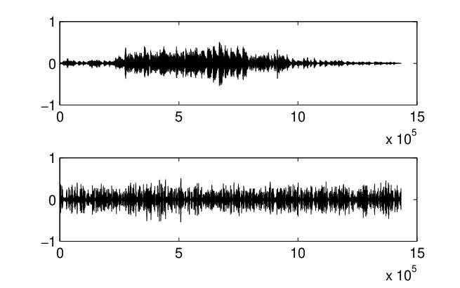
Given a signal split it into blocks of size . Apply an invertible random permutation to scramble the block’s location (the bottom graph in Figure 3 provides a visual illustration of how the signal in the top graph looks after this step). Let’s denote the re-arranged signal by .
- ii)
Group every of the blocks to have segments .
- iii)
Approximate each of the segments independently of the others, as it each segment were an entire signal, i.e., obtain .
- iv)
Assemble the segments to have the approximation of the whole signal as .
- v)
Reverse the permutation of the block’s location to obtain, from , the approximation of the original signal .
Numerical Example IV
The signal to be approximated is a 32.5 secs
(1433600 samples) piece of
Piazzola music, shown in the top graph of Figure 3. It is
partitioned into blocks
of 1024 points each. After randomization (bottom graph of
the same figure)
the blocks are grouped into
50 segments, each of which is independently
approximated by the HBW-OMP/OOMP approach to produce
a SR=11.53.
The resulting SNR of the approximated signal
is 29.12 dB with HBW-OMP and 30.15 dB with HBW-OOMP.
Equivalent approximation quality
is obtained with
other realizations of the random process. For
appreciation of this result the original signal
was also approximated by HBW-OMP/OOMP,
but without segmentation.
In that case the quality corresponding to SR=11.53 is only
higher (SNR=29.66 dB with HBW-OMP and SNR=30.73 dB
with HBW-OOMP). The conclusion is that, even if the
largest the segments the less the distortion
for the same sparsity, applying HBW-OMP/OOMP on segments
of a large signal may be still significantly
more advantageous
than the independent approximation of the blocks. Indeed,
in this example the
latter yields a SNR of 25 dB with OMP and 26.1 dB
with OOMP.
5 Conclusions
Cooperative greedy pursuit strategies
for approximating a signal partition
subjected to a global constraint on sparsity have been
considered. The cooperation between
partition units was realized in several ways:
i)By ranking the partition units for their sequential
stepwise approximation (HBW-OMP/OOMP) ii)By ranking the partition units for stepwise downgrading of the whole
approximation (HBW-BOOMP) iii)By allowing for
downgrading of some partition units (donors) and
upgrading of another partitions units (receivers),
to improve the approximation
quality (HBW-SbR-OMP/OOMP). Comparisons of the OMP and OOMP
criteria indicate that for the type of dictionaries
and signals considered here, the OOMP criterion
renders improvements of sparsity up to 20
in relation to the equivalent strategy involving
OMP.
The HBW algorithms maintain the complexity comparable
with the
totally independent approximation of each partition unit.
The examples presented here, using
trigonometric dictionaries for achieving high quality
approximation of musics
signals, provide a clear illustration of the
benefits arising by the proposed strategies. Indeed, for
a piano melody
the increment in sparsity is 128 higher than
the sparsity produced by approximating each partition
unit up to same quality. Comparison of trigonometric
dictionaries results, against results
obtained with trigonometric basis, give an improvement of
equivalent order: 133. The mixed Cosine-Sine dictionary
has yielded the best sparsity results, not
only for the test signals included in this paper but
for a significant number of
other signals, all in the category of melodic music.
Because the proposed HBW implementation of pursuit
strategies
requires storage of order ( being the
length of each block in the partition and
the number of total atoms to approximate the whole signals)
a simple procedure for processing large signal was proposed:
Previous to dividing the signal
into independent segments, each of which to be approximated
with the identical constraint of sparsity,
the randomization of the
partition units is advised.
Appendix A
References
- [1] B. K. Natarajan, “Sparse Approximate Solutions to Linear Systems”, SIAM Journal on Computing, 24, 227–234 (1995).
- [2] S. S. Chen, D. L. Donoho, M. A Saunders, “Atomic Decomposition by Basis Pursuit”, SIAM Journal on Scientific Computing, 20, 33–61 (1998).
- [3] J. H. Friedman and W. Stuetzle, “Projection Pursuit Regression”, Journal of the American Statistical Association, 76, 817–823 (1981).
- [4] S. G. Mallat and Z. Zhang, “Matching Pursuits with Time-Frequency Dictionaries”, IEEE Trans. Signal Process., 41, 3397–3415 (1993).
- [5] Y.C. Pati, R. Rezaiifar, and P.S. Krishnaprasad, “Orthogonal matching pursuit: recursive function approximation with applications to wavelet decomposition,” Proc. of the 27th ACSSC,1, 40–44 (1993).
- [6] Y. Eldar, P. Kuppinger and H. Biölcskei, “Block-Sparse Signals: Uncertainty Relations and Efficient Recovery”, IEEE Trans. Signal Process., 58, 3042–3054 (2010).
- [7] D. L. Donoho , Y. Tsaig , I. Drori , J. Starck, “Stagewise Orthogonal Matching Pursuit”, IEEE Transactions on Information Theory, 58, 1094–1121 (2006).
- [8] D. Needell and J.A. Tropp, “CoSaMP: Iterative signal recovery from incomplete and inaccurate samples”, Applied and Computational Harmonic Analysis, 26, 301–321 (2009).
- [9] D. Needell and R. Vershynin, “Signal Recovery From Incomplete and Inaccurate Measurements via Regularized Orthogonal Matching Pursuit”, IEEE Journal of Selected Topics in Signal Processing, 4, 310–316 (2010).
- [10] D. L. Donoho, “Compressed sensing”, IEEE Trans. Inf. Theory,52, 1289–1306 (2006).
- [11] E. Candès, J Romberg, and T. Tao, “Robust uncertainty principles: exact signal reconstruction from highly incomplete frequency information,” IEEE Trans. Inf. Theory, 52, 489 –509 (2006).
- [12] R. Baraniuk, “Compressive sensing”, IEEE Signal Processing Magazine, 24, 118–121, (2007).
- [13] E. Candès and M. Wakin, “An introduction to compressive sampling”, IEEE Signal Processing Magazin, 25, 21–30 (2008).
- [14] R. Baraniuk, “More Is less: Signal processing and the data deluge”, Science, 331, 717–719 (2011).
- [15] L. Rebollo-Neira, R. Matiol, S. Bibi, “Hierarchized block wise image approximation by greedy pursuit strategies,” IEEE Signal Process. Letters, 20, 1175–1178 (2013).
- [16] L. Rebollo-Neira and D. Lowe, “Optimized orthogonal matching pursuit approach”, IEEE Signal Process. Letters, 9, 137–140 (2002).
- [17] M. Andrle and L. Rebollo-Neira, “A swapping-based refinement of orthogonal matching pursuit strategies”, Signal Processing, 86, 480–495 (2006).
- [18] http://www.nonlinear-approx.info/examples/node01.html
- [19] K. Kreutz-Delgado, J. F. Murray, B. D. Rao, K. Engan, T. Lee, and T. J. Sejnowski, “Dictionary learning algorithms for sparse representation”, Neural Comp., 15, 349 – 396 (2003).
- [20] M Aharon, M Elad, and A Bruckstein, “K-SVD: An Algorithm for Designing Overcomplete Dictionaries for Sparse Representation”, IEEE Transactions on Signal Processing, 54, 4311–4322 (2006).
- [21] R. Rubinstein, M. Zibulevsky, M. Elad, “Double Sparsity: Learning Sparse Dictionaries for Sparse Signal Approximation”, IEEE Trans. Signal Process. 58, 1553–1564 (2010).
- [22] I. Tos̆ić and P. Frossard, “Dictionary Learning: What is the right representation for my signal?”, IEEE Signal Process. Magazine, 28, 27–38 (2011).
- [23] L. Rebollo-Neira, J.Bowley Sparse representation of astronomical images, Journal of The Optical Society of America A, 30, 758–768 (2013).
- [24] M. Andrle, L. Rebollo-Neira, E. Sagianos, “Backward-optimized orthogonal matching pursuit approach”, IEEE Signal Proc. Let.,11,705–708 (2004).
- [25] L. Rebollo-Neira, “Backward adaptive biorthogonalization”, Int. J. Math. Math. Sci. 1843–1853 (2004).
- [26] Å. Björck, “Numerical Methods for Least Squares Problems”, SIAM, Philadelphia, 1996.
- [27] G.W. Stewart, “On the stability of sequential updates and downdates”, IEEE Trans. Signal Process., 43, 2642–2648 (1995).