Magnification of signatures of topological phase transition by quantum zero point motion
Abstract
We show that the zero-point motion of a vortex in superconducting doped topological insulators leads to significant changes in the electronic spectrum at the topological phase transition in this system. This topological phase transition is tuned by the doping level and the corresponding effects are manifest in the density of states at energies which are of the order of the vortex fluctuation frequency. While the electronic energy gap in the spectrum generated by a stationary vortex is but a small fraction of the bulk superconducting gap, the vortex fluctuation frequency may be much larger. As a result, this quantum zero-point motion can induce a discontinuous change in the spectral features of the system at the topological vortex phase transition to energies which are well within the resolution of scanning tunneling microscopy. This discontinuous change is exclusive to superconducting systems in which we have a topological phase transition. Moreover, the phenomena studied in this work present novel effects of Magnus forces on the vortex spectrum which are not present in the ordinary s-wave superconductors. Finally, we demonstrate explicitly that the vortex in this system is equivalent to a Kitaev chain. This allows for the mapping of the vortex fluctuating scenario in three dimensions into similar one dimensional situations in which one may search for other novel signatures of topological phase transitions.
I Introduction
Topologically distinct phases which cannot be classified by the classical Landau paradigm comprise some of the most recently discovered states of matter[1, 2, 3]. An important signature of these topological phases is the appearance of novel, low-energy, robust, edge states; one such state is the so-called Majorana bound state at the edges of topological superconductors [4]. As ubiquitous signatures, the detection of these neutral fermions has been the main trend in the characterization of particle-hole symmetric topological phases. Although evidences of Majorana fermion physics have been identified in tunneling [5] and scanning tunneling microscopy (STM) measurements[6], the interpretation of their signatures is controversial in many cases, as the imprints from the topological regime are often mixed with signals from disorder and extra undesired quasiparticles.
While the aforementioned gapless edge states act as a signature of topologically non-trivial regimes, the signatures of the transition from a topologically trivial to a topological phase present themselves in the bulk by the closing and re-opening of the excitation energy gap[7, 8, 9]. In many of the proposed systems which can be tuned through a topological phase transition (TPT), the excitation gap is very small compared with experimental resolutions and cannot be probed directly.
In this work, we show that quantum fluctuations can shift the spectral weight in the density of states of a given system before and after a TPT to further separated energies and, as a result, magnify the change of the spectrum resulting from this process. This situation will be relevant as long as the sample’s temperature is below , where is the pinning frequency and is Boltzmann’s constant. We discuss this effect in the context of the chemical potential induced topological phase transition in the vortices of superconducting doped topological insulators. In this particular situation, we also demonstrate how the effects of Magnus forces on the vortex dynamics[10] have a novel signature in the spectral change at this TPT, exposing the pumping of vortex modes responsible for the phase transition, as described below. Our results are general, however, and can be extended to other types of topological phase transitions. To demonstrate this, we present a way to map the 3D situation into a 1D setting in terms of wire networks which may be used to probe for the topological phase transition of actual Kitaev chains, Su-Schrieffer-Heeger chains and other unidimensional topological chains.
To understand how quantum fluctuations affect vortices in superconducting doped TIs we start by discussing vortex dynamics in regular superconductors (SCs). This physics has been widely studied[11, 12] and, given the natural length scale of vortices, their different properties might display both classical and quantum phenomena. Within the BCS theory of superconductivity, an stationary vortex affects the spectrum of the superconductor by generating in-gap modes localized around and along the vortex core[13]. The energy of these discrete bound states, known as Caroli-de Gennes-Matricon (CdG) modes, is given by where is the size of the bulk SC gap, is the fermi energy and is an integer. The signatures of these in-gap states have been experimentally observed by STM measurements[14, 15]. In practice, however, even though the spatial resolution of STM is well within the size of the vortex modes[16], given the small size of their so-called mini-gap, , the energy of each single mode is hard to be resolved and usually multiple modes are observed together[14].
It is well known that the pinning of vortices is necessary for the stability of type-II SCs. The discussion above would be the final status of the problem for pinned vortices, were they absolutely static. Although a pinned vorticex has a fixed position at the sample, even at the lowest temperatures, their quantum zero point motion cannot be ignored. Interestingly, it was shown that such quantum fluctuations affect the quasiparticle spectrum, moving part of the spectral weights of the in-gap vortex modes to the frequencies associated with vortex fluctuations[17, 18, 19]. We then contend that exploiting this ubiquitous quantum mechanical phenomenon to probe for TPTs is a promising idea, leading to novel signatures of these transitions.
To test this approach, superconducting doped TIs arise as the most natural test ground. The discovery of superconductivity in doped TIs triggered several studies, particularly because of the suggestions that doped TIs might realize topological superconductivity[20, 21, 22, 23, 24]. Theoretical studies of superconductivity in the surface states of TIs started even before the experimental realization of bulk superconductivity in doped TIs, when it was shown that, theoretically, if superconductivity is induced in their helical surface states, vortex modes will include a zero-energy Majorana bound state[25]. In the context of bulk superconducting doped TIs, it was later shown that the Majorana mode at the ends of a vortex line persist up to a critical value of doping in these systems as well[26, 27, 28]. At this critical doping level, the two Majorana modes at the ends of the vortex hybridize and become gapped. The presence or absence of Majorana modes at the end of the vortex line contrast the two topologically distinct phases. In fact, the vortex in doped superconducting TIs becomes effectively equivalent to a Kitaev chain, one of the pioneering theoretical models to realize topological phases and phase transitions with Majorana edge states[29] (check also Section V of the present work).
As desired, the signature of this TPT also shows up in the spectrum of the states extended along the vortex. The original mechanism lies in the CdG modes. The important property of these states is that they are gapped by the small energy scale of the mentioned mini-gap. This energy protects the surface Majorana zero modes, confining them to the surface of the sample. Because of strong spin-orbit coupling and the resulting band inversion of TIs[30], the Fermi surface here has non-trivial topological properties which show up as a non-zero Berry connection. The CdG modes then inherit this Berry phase as a modification to their energy spectrum, which also separates in two sets due to the existence of two degenerate TI Fermi surfaces, which becomes . Here is the Berry phase around the curve on the Fermi surface defined by setting the wave-vector along the vortex line equal to zero. In this case, when , and the zero energy surface Majorana modes at the ends of the vortex can merge through the gapless mode which is now extended along the vortex. The richness introduced by spin-orbit coupling and topology in this system leads to the signatures that we demonstrate.
For the physical picture of a fluctuating vortex to be reasonable, its position and cross-section structure must be well defined. Testing with some real numbers, Copper doped was the first topological insulator found to become superconducting upon doping, at 3.8 [20]. One must spatially resolve the local density of states (LDOS) at the vortex core which, as we demonstrate, comes from the and CdG modes. Their maxima lie at and are separated from the next closest mode (with ) by the Fermi wavevector scale , which is well within the resolution of STM. Regarding the energy scales, the change of spectrum at the TPT happens at the mini-gap energy scale . This is very small compared to the spectral resolution of STM which is of the order of the measurement temperature ()[16]. It is then clear that an important obstacle to the verification of topological phase transitions in this system by STM is the small excitation gap. Overcoming this energy scale problem is the main role of the vortex position fluctuation we analyze.
The paper is organized as follows. In Section II we explain the model in which we base our calculations. In Section III we follow Ref.[17], showing how the vortex fluctuations induce a self-energy correction which redistributes the peak weights in the LDOS for our specific model. This affects directly the tunneling conductance measured in STM experiments and in Section IV we demonstrate what are the novel consequences of this phenomenon for the vortex TPT in doped TIs. We believe that the approach we describe in the bulk of our paper is generalizable to other situations and we dedicate section V to stipulate how to translate the ideas from the 3D context to 1D situations concerning Kitaev chains or other linear or quasi-linear topological phases. We conclude in Section VI. As computations are a bit involved, we avoid displaying them throughout our narrative as much as we can. We refer the reader to the appendices, where details are displayed thoroughly, whenever necessary.
II Fluctuating vortex model
Superconductivity and the vortex quantum phase transition (VQPT) in doped topological insulators may be understood in the weak pairing limit (, where is the SC coherence length)[26]. In this regime, a gradient expansion can be deployed to study the effects of the fluctuating vortex position in the low-energy spectrum[17].
We start with an action of the form . The first term is a Bogoliubov-de Gennes (BdG) action for the superconducting doped TI,
| (1) |
where
Here is the chemical potential and the effective low energy 3D TI Hamiltonian is given by
| (5) |
with Nambu-spinor and where . are orbital indices and and Pauli matrices act on orbital and spin Hilbert spaces, respectively. The superconducting pairing contains a vortex profile centered at a fluctuating position whose dynamics is governed by[17]
Physically, the action () describes a particle of mass oscillating in an harmonic trap of frequency which depends on the properties of the trapping potential [17]. This oscillator frequency dictates the qualitative features of the energy peak distribution of the LDOS. Finally, corresponds to a Magnus force acting on the vortex. The frequency will be shown to play an essential role, introducing an energy scale for the chemical potential in which we have distinguished signatures of the VQPT in the system’s LDOS.
To capture the coupling between electronic excitations and vortex fluctuations, we expand the superconducting pairing around the vortex rest position . This approximation is valid at weak-coupling [17], which is also the regime of validity of Hamiltonian (II). Within this formalism, the full problem is described by a perturbative action is given by (1) with the BdG Hamiltonian in the stationary vortex limit, (explicitly given in (96)). The interaction term is given by
| (10) |
The interaction between vortex modes and the fluctuations in the vortex position leads to a self-energy correction to the energy of the CdG modes.
III Perturbed LDOS
Assuming a singlet intra-orbital pairing for doped TIs, the VQPT was found originally by an exact diagonalization of lattice toy models and a semi-classical study of the BdG mean-field Hamiltonian [26], as well as numerically solving the self-consistent BdG equations[28]. In order to study the effects of vortex fluctuations on the LDOS, it is convenient to use a basis which diagonalizes the Hamiltonian at the limit of a static vortex. Thus, we first present the VQPT by a novel real-space diagonalization of the BdG equation of Hamiltonian (96) following the ideas from [31]. The details follow in Appendix A.We expand the Grassmann fields in terms of eigenvectors of the static-vortex BdG Hamiltonian as . The eight arising bands obey where and labels conserved quantum numbers. Precisely, represents a generalized angular momentum , which commutes with the Hamiltonian (see [26] or Appendix A), while labels the different eigenstates of the radial BdG equation at fixed . At weak coupling, we further project into the two bands which cross the doubly degenerate Fermi surface of . Labeling these states by , we have, at low energies, with
The numerical diagonalization may be done replacing the infinite system with a disk of finite radius with a profile for the vortex and solving the secular equation for the Fourier-Bessel coefficients and (details follow in Appendix A and references therein.)
To study the VQPT we consider the lowest energy vortex modes. These are the CdG modes and allow fixing the label , which we drop. The two sectors (labeled by ) are connected by particle-hole (PH) conjugation operator ( is the complex conjugation operator) as . The energies of the CdG vortex modes in this case are the expected[26]
| (37) |
so that . Here is the Berry phase calculated around the Fermi surface on the curve with zero wavevector along the vortex[26]. As the chemical potential increases, the Fermi surface enlarges and varies from to , defining a critical chemical potential such that . Our results for the energies of the CdG modes, which are presented in Fig. 1, are consistent with the previous study of the phase transition in Refs. [26] and [28].
In terms of the CdG eigenstates, equation (10) is written
where
| (39) |
Vortex fluctuations then generate the following self-energy for CdG vortex modes which we calculate using the GW approximation[32] (details follow in Appendix B),
| (40) |
Here are reduced matrix elements with and For unit vorticity, angular momentum conservation implies that is connected only to by such interactions. The energy scale introduced by ( and dominated by as aforementioned), represents a “magneto-plasma” frequency in an Einstein model[17]. In Appendix B, we present closed formulas for these matrix elements.
One finally needs to evaluate the LDOS,
| (41) |
where is a -particle ground-state, is an -particle excited state (with generic quantum numbers ) and is an electronic state creation operator at level in sector . Using the vortex-modes eigenbasis, this can be written, taking into account the effects of the vortex fluctuations in the self-energy, as
| (42) | |||||
| (43) | |||||
| (44) |
Through the perturbative interaction, the energy density profile of CdG modes is modified with part of the spectral weight from being transfered to new “satellite” peaks in the LDOS [17]. Both the spectrum and the profile of dramatically change the phenomenology described by (44) when the parent metallic state of the superconductor comes from doped TIs, as compared with ordinary metals.
IV Tunneling Conductance Analysis
The local tunneling conductance is found, at low temperatures, by convolving the LDOS (44) with the derivative of the Fermi distribution function as
| (45) |
The normalization constant assumes an STM tip with constant DOS (for a free 2D electron gas) with the corresponding tunneling conductance , and is the Fermi-Dirac distribution. At very low temperatures, the tunneling conductance is equal to the LDOS, however still smoothed by the finite temperature effects.
Given the atomic level resolution of STM, we can safely focus at the density of states at the vortex core . As seen in (III) and (III), the wavefunction components may be expanded in terms of Bessel functions. In particular, at , only Bessel functions of order zero have non-zero amplitude while all the other Bessel functions vanish. From our Fourier-Bessel expansion of the CdG modes above, only and, as a result of spin-orbit coupling, modes have finite contributions in at the origin.
The states have energies . These energy levels may be pumped from negative to positive values (and vice versa) by changing the chemical potential, evolving the Berry phase from to . This novel feature leads to a change of sign in the factors of in the self-energy given in (40) when , which determine the energies of the satellite peaks. As a result, the TPT manifests itself by a discontinuous change in the density of states by energies of order to energies of order .
Remarkably, the local spectrum at the vortex center breaks particle-hole symmetry. The origin of this lies in the spin-orbit coupling which, together with the BdG doubling, filtered only the states at this position, leaving out the states. Naturally the full DOS is PH symmetric. These points will be considered again in Sec. V in the context of the effective theory for the vortex bound states after integration in the radial and angular directions.
Even more importantly, one notes that the Magnus force term associated with the vortex motion, whose amplitude is proportional to , breaks the mirror symmetry which is connecting the PH sectors of the CdG modes. As a result, the discontinuous transition of energy of the CdG modes from the two sectors does not happen simultaneously at the same value of doping for both cases. This is essential for the change in the LDOS to be seen in this context, as it provides an energy window over which the density of states at the energy of vortex oscillations is remarkably modified by the TPT. It is also important to note that, for other CdG modes (such as the mode with whose maximum amplitude is at away from the center of the vortex), the opposite transition will happen. Given the spatial resolution of STM, however, the different modes should be resolvable.
To make the above claims regarding the peak-jumping less abstract, let us concretely analyse the relevant contributions to the self-energy. As discussed, from angular momentum conservation, and from we can read the corresponding result for . These simplifications allow us to reduce the self-energy to just a couple of relevant pieces,
| (46) |
and
| (47) |
To find the positions of the peaks, one solves
| (48) |
The solutions are clearly sensitive to the sign of As we do not have an estimate for the actual strength of the Magnus effect, to be definite, we take . It is a simple job to notice that and , for any value of the chemical potential. The sign of , however, does depend on . This allows one to define a value at which changes. The structure of depends crucially on this. From the CdG spectrum (37), we set explicitly, finding
| (49) |
where is the Berry phase. As this phase grows monotonically from to , it is clear that the sector has a sign change at values of larger than those of the sector, as long as . In sum, this determines when each set of peaks will jump as function of . In Appendix C we explore this further, also showing analytically that, at , only the leftmost satellite peak from will jump due to this sign change.

Figure 2 displays our main results. It shows the differential conductivity at the vortex center (more details on numerical parameters used here are given in Figure 4 in the appendix). Angular momentum conservation implies that each non-interacting energy level unfolds into a set of three peaks.
We present the differential conductance for three ranges of chemical potential , in blue, and , in red, and in blue again, which appears to be identical to . This happens because the separation of the central peaks from is , which cannot be resolved close to the phase transition (just as the peaks from cannot be resolved at this situation.) In this situation, having a finite is crucial to observe all peaks and the discontinuous effects of the topological phase transition. The pattern in the LDOS should be, for each and sector , of a large central peak located at with the two partners offset approximately by with . In our case, a total of 12 peaks is expected for each value of the chemical potential (3 from , another 3 from and twice this due to the two sectors), not all of them being resolvable due to thermal effects. The large peaks closest to correspond to . The strength of the respective satellite peaks is suppressed by a factor, where is the coherence length [17]. An inset displays the position of these peaks.
A remarkable behavior develops in the sattelite peaks (the rightmost small peaks at negative and positive frequencies). This is evidenced by the solitary blue peak at positive . It corresponds to the contribution coming from , whose position jumps from this value by approximately as the chemical potential pumps the negative energy state at into positive energies after crossing . Similarly, when moves above , the peak from jumps by . In appendix C we demonstrate that the approximate positions of the peaks can be determined analytically.
Concerning the magnitude of the Magnus effect, if , the effects from the Magnus force are sub-dominant to the CdG energy gap and the sensibility to which one needs to tune the (zero-temperature) chemical potential may again be beyond technical realization at the current time. If , on the other hand, as the evolution of the Berry phase is from to , the critical chemical potentials may not be captured as one tune and one will be bound to the regime of , which is similar to the standard s-wave case (except for the multiplicities of peaks and apparent breaking of the PH constraint.) As this seems to critically constrain the actual visualization of these effects in practice, we proceed now to consider some different situations in which one may actually control the energy difference between the states for different sectors. In this case, we will see that if this energy difference can be made larger, even at one may be able to capture the closing and reopening of the energy gap from .
V 1D wire mapping
To conclude our considerations, we would like to speculate about the realization of similar signatures of TPTs by quantum motion in other systems. Here we demonstrate concretely the claim from [26] stating that the vortex in superconducting doped TIs presents a topological phase transition equivalent to a Kitaev wire. We then proceed to showing that, more generally, the Hamiltonian projected at the vortex states corresponds to a set of wires (or a single multiband wire) inheriting a first neighbor mutual coupling from the vortex fluctuations in 3D. We then identify the important ingredients necessary to realize the discussed phenomena in the context of 1D topological systems.
V.0.1 Vortex Hamiltonian projection
Start with Hamiltonian (96) from the appendix, keeping the -direction terms. We also keep the vortex fluctuations to first order in the gradient of the superconducting pairing. We have
| (50) | |||||
| (51) |
We are going to project this into the lowest energy sectors from (III) and (III). At finite z, we have , choosing the CdG states with . We will project the radial part the Hamiltonian to find out what Hamiltonian gives the equations of motion for . Considering the sectors then we have
| (52) | |||||
Notice that as , the fluctuating vortex potential becomes diagonal with respect to the sectors. This result is the same as we had found in our considerations at vanishing and we already know what this term looks like,
with
Due to the vortex structure in , we are only coupling to .
Now we project . To keep the notation short, we introduce Dirac matrices and as in the appendix. It is easy to see that terms linear in contribute off-diagonal in the sectors while terms quadratic with contribute only diagonally. For these diagonal terms, we develop couplings
| (67) |
Importantly, the sign of these couplings is the same and the angular integration enforces . For the off-diagonal terms we develop the couplings
| (68) |
V.0.2 1D Wire network
Adding up the matrix elements above gives the projected Hamiltonian
For Hermiticity . For the diagonal terms we may still use to write
As the signs of are the same, one can easily see that the Hamiltonian is essentially the same as a Kitaev chain. For , on the other hand, the Hamiltonian does not describe a Kitaev chain. The PH symmetry is only present when both , besides the sectors, are taken into account. In this 1D projection, the contributions of the states in the whole radial direction are taken into account; in contrast, when probing the 3D system’s LDOS at the center of the vortex, we filtered the contributions of and only. Because of this, PH symmetry is apparently broken in Figure 2. These considerations are more clearly seen by writing
| (87) | |||||
The term does not vanish here (unless ), as usually happens. To see that indeed the system is PH symmetric, one has to take into account the full second quantized Hamiltonian with all pairs.
Likewise as above, the fluctuations may be written
They couple diagonally in the indices and also bring up an apparently PH breaking term.
This projected Hamiltonian is then equivalent to a p-wave wire network. This is a very unusual network as PH symmetry actually connects different wires while each wire has PH symmetry actually broken. Although unusual, however, similar ideas have been considered in the literature [34]. It is remarkable, in any case, that the 3D physics we started with ends up in such an exotic 1D scenario.
V.0.3 TPT signatures in 1D
From the above results, we may identify the minimal ingredients necessary to magnify the signatures of TPTs in 1D systems by a mechanism similar to as considered in the vortex case. This minimal set of ingredients is undemanding. We list them in the context of Kitaev chains, as there seems to be a recent focus of interest in the literature concerning Kitaev wires networks (see [35], for example). We stress, however, that the same ingredients would suffice for other 1D topological systems, such as Su-Schrieffer-Heeger wires or Kitaev superconducting
- 1.
A pair of gapped wires, one of which tunable through a TPT;
- 2.
A diagonal fluctuating coupling between them;
With these, one may reconstruct the important features of Eqs.(87) and (V.0.2). This situation is illustrated in Figure 3.

Notice that the broken (PH) symmetry found in the projection on the vortex modes in the 3D scenario is not fundamental and is not included in our minimal list. It implies but a shift in the peaks in the spectrum, like as in the large peaks from in Fig. 2, and hence is unimportant. Also, a single pair of Kitaev chains is enough (the effects from and in (46) and (47) are not important). This pair of wires could also be substituted by a single wire with a pair of low energy bands. The tight-binding model for this is written
| (91) |
where are the chemical potentials, are the SC pairings, are the corresponding SC phases and the hopping amplitude for each wire. The index labels the two chains. Upon BdG doubling, it is easy to demonstrate that this reduces to (87) in k-space, without the term.
As for the fluctuation part of the Hamiltonian, one may have simply
| (92) |
for a fluctuating coupling . This should lead to similar self-energy corrections to the wires energies as (46) and (47), namely
| (93) |
and
| (94) |
where gives the two Nambu components. The fluctuation frequency of determes the new large energy scale. To find the positions of the peaks, one solves again
| (95) |
which now leads to a single sattelite peak for each energy level.
Importantly, the effects of the Magnus force are not necessary in the 1D case and, hence, a single fluctuating parameter is enough. This happens because one may (by ramping the chemical potential transversally to the wires, for example) keep a single wire well away from the phase transition with a large gap. Suppose, for example, wire is kept with a large gap. In this case, the sattelite peaks from the two sectors in this wire will stay always far away from each other. This way, by tuning the chemical potential from wire , one can verify its phase transition by probing for the jumping in the satellite peaks of wire .
As a final comment, out of the p-wave superconductivity context, one might work similarly with a set of Su-Schrieffer-Heeger (SSH) wires. In this case, the Hamiltonian will be similar to as the BdG Hamiltonian considered so far, with the caveat that the Nambu spinor now should be substituted by an ordinary spinor for a sublattice pseudo-spin degree of freedom. The gapping parameters in this case will be given by staggered hopping amplitudes and chemical potentials. Formally, the problem is the same and one may extend the results discussed so far to this situation.
VI Conclusions
Quantum fluctuations of vortex positions are ubiquitous and should manifest themselves at very low temperatures. We found out that, in the context of doped three dimensional topological insulators these fluctuations may be exploited to magnify the signatures of topological vortex quantum phase transitions. This manifests at the LDOS at the vortex core by energy peaks which discontinuously jump as function of the chemical potential. This finding also determined characteristic features of the low-energy Caroli-de Gennes-Matricon modes in this system which make them stand out as very distinct from standard s-wave Caroli-de Gennes modes, such as their spatial distribution and effects in the LDOS at the vortex core. Finally, our results also point to the possibility of capturing the effects of Magnus forces acting on the vortices, whose magnitude is directly related to the chemical potential values in which the topological phase transition induces peak position shifts.
The frequency of the position fluctuations plays an important role as it sets the scale of the peak jumps. In the context of high temperature superconductors, there are reports of this energy scale going up to meV[37]. It is important to point out that this frequency can be controlled to some extent and indeed increased depending on the properties of the vortex pinning potential. Recent developments in doping TIs with Niobium, which leads to the formation of magnetic moments in the bulk superconducting TI, can provide stronger pinning and so larger frequencies for the vortex fluctuation[33]. Measured physical values of the vortex fluctuation frequencies and Magnus force frequency in this system are not known to us at this point.
Cryogenic STM measurements are fundamental to uncover the discussed signatures. Situations with lighter and smaller vortices, whose zero-point motion effects would be stronger, could also be arranged as the vortex size is known to be strongly sensitive to temperature and magnetic field strength [36]. For vortices of too minute sizes, however, the Taylor expansion method deployed here to derive the interactions is not precise. In such cases, different approaches to the problem, such as used in [18], are necessary in order to obtain trustworthy predictions. Also, a proper account for the effects of dispersion along the vortex may need detailed attention. It is beyond the scope of this work to consider these.
Finally, we studied the local physics along the vortex core. Projecting the Hamiltonian with the Caroli-de Gennes-Matricon wavefunctions we demonstrated explicitly that the vortex line behaves as a Kitaev chain, with the corresponding topological phase transition. Further studying how the vortex position fluctuations are projected into this system allowed us to find some key ingredients which one may use to obtain new signatures of topological phase transitions in one-dimension. A promising scenario lies in the study of the density of states upon fluctuations of the transversal coupling between a pair of neighboring gapped wires. Again, effects of dispersion along the wires still deserve attention.
Acknowledgments
The authors acknowledge insightful discussions with V. L. Quito, S. Sachdev, S. Gopalakrishnan, V. P. Nair, M. Sarachik and A. P. Polychronakos. PLSL acknowledges support from FAPESP under grant 2009/18336-0.
Appendix A Caroli-de Gennes modes
Here we present our numerical method to derive the spectrum of vortex modes for a stationary vortex in doped superconducting topological insulator [26], and compare the solutions with an analytical approximated ansatz. The latter will be used to study the effect of vortex quantum zero-point motion on the vortex spectrum.
The method which we apply is analogous to the one introduced by [31] and [17] in the context of ordinary superconductors. We start by considering a cylinder space, infinite in the direction. The Bogoliubov-de Gennes Hamiltonian with a static vortex centered at the origin reads
| (96) |
where the ”Dirac velocity” is set to one throughout our derivations and recovered to simplify the numerical calculations later. The Dirac matrices obey and Notice commutes with the kinetic Hamiltonian and is not a “mass” term. In our basis, a choice for the representation follows
| (97) | |||||
| (98) |
with Nambu, orbital and spin spaces described by and Pauli matrices, respectively. Here gives the pairing with a profile, to be concrete.
The vortex runs along the direction and translation invariance allows us to consider the momentum; with the understanding that only are topologically relevant, we take since we are looking only for the low energy Caroli-de Gennes-Matricon modes [26].
The Hamiltonian commutes with the generalized angular momentum operator , where . This allows writing the solution spinors as
| (99) |
where is an integer representing the standard angular momentum and labels the many possible energies for a given . At , the Hamiltonian obeys a further symmetry given by . Noticing that and naturally , we see that the eigenvalues of also label particle and hole partners. This allows one to separate in four-spinors , obeying corresponding Schrodinger’s equations with projected Hamiltonians [26],
| (100) |
We focus in , noticing that with . The reduced radial Hamiltonian reads
| (101) | |||||
Here Pauli-matrices represent a spin-orbital coupled space. Noticing that
| (102) | |||||
| (103) |
act as operators which lower and raise the level of Bessel functions (and gives the Bessel differential operator itself), it is easy to find a proper basis to expand the states. If , we recover a pair of topological insulator Hamiltonians with spectra given by , with and a “radial linear momentum” quantum number. In the weak pairing approximation, since we are interested only in the lowest energy modes, we solve for the eigenstates of the TI Hamiltonian using the ladder operators above and project out the bands from and . Thus Fourier Bessel expanding the radial wavefunctions as
| (104) |
where
and are normalization constants given by The Schrodinger’s equation reduces to
where
| (113) |
with respective signs,
| (114) |
and the spinor is
In terms of our original variables, the wavefunctions are then written
where
| (123) | |||
and the mirror (particle-hole) partners are built from .
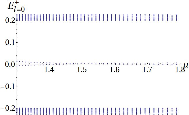
We then fix a finite radius for the cylinder size which forces us to discretized where are the -th Bessel zeroes at each subspace. We fix a UV cutoff at some (large) -th Bessel zero. Diagonalizing the resulting Hamiltonian leads to the spectrum shown in 4. One sees two in-gap modes, one corresponding to outer edge modes, which we neglect, while the other corresponds to our desired vortex modes, as can be checked by plotting their respective probability densities.
For the low energy states, (a label which we drop from now on), one may check that the spectrum follow the expected
| (130) |
where is the chemical potential dependent Berry’s phase. At the critical chemical potential . It grows monotonically from to with the chemical potential. Noticing that the values of the momentum in -space are strongly localized at its Fermi value , as one might expect, it is easy to guess an analytical approximation for the wavefunctions which satisfies their desired asymptotic behaviors (see [26] for details). We have
| (131) |
where
| (137) | |||
and the new normalizations read
| (144) |
Here, is a normalization constant of order . In the main text we compare the analytical and numerical results for the wavefunction at and , showing that the approximation indeed works.
Appendix B Electronic Effective Interaction and Self-Energy
In this section we compute explicitly the electronic self-interaction due to the interplay with the vortex fluctuations and the corresponding self-energy in the GW approximation.
We start from the vortex effective action of the main text in frequency space
and work at zero-temperature. Noticing that , we introduce a basis which diagonalizes the Lagrangian density as
with
| (152) |
and the Green’s functions . This sets the two important energy scales dictated by the vortex fluctuations as , from the Magnus force, and , from the harmonic trap.
As discussed in the former section, the low-energy modes divide into two Hilbert space sectors related by a -mirror/particle-hole symmetry. Each sector is subject to an effective potential arising after the integration of the vortex 0D field theory. From equations we may write:
| (153) |
Define and rewrite the scalar products in terms of the coordinates and , with . Then
| (154) |
This allows, with a careful consideration of positive and negative frequencies, integration over the vortex degrees of freedom, leading to the effective action of the electronic modes as
| (155) | |||||
where . A tedious but straightforward simplification leads to the effective electronic self-interaction
| (156) | |||||
where
| (157) |
From (A), the matrix elements have a simple form
| (158) |
which also shows the convenient fact that .
Interaction (157) shows a screened Coulomb-like retarded interaction. The self-energy in the GW approximation comes now from a simple 1-loop calculation
| (159) | |||||
The first term vanishes. The second must be considered with care as the pole structure is sensitive to the structure of the energy levels. An integration over the complex plane gives the self-energy of the main text
| (160) |
where and .
To calculate the matrix elements one may make use of the Feynman-Hellman relations, adapted to our Hamiltonian and in a finite cylinder. A long calculation making full use of Bessel function relations gives finally
with
| (162) |
and
| (163) |
Here, is the cylinder finite radius, is the j-th zero of the l-th Bessel function and with . The other matrix elements may be found from
| (164) | |||||
| (165) |
These expressions are very similar to Bartosch’s, corrected for spin-orbit coupled states.
Appendix C Peak Analysis
Here we describe in detail the determination the relative sizes and positions of the tunneling conductance peaks. We start rewriting,
| (166) | |||||
| (167) |
using the vortex-modes eigenbasis. STM measurements probe the tunneling conductance
| (168) |
where is the Fermi distribution.
At zero-temperature this reduces simply to the LDOS, up to a constant. At finite temperature we may write
| (170) | |||||
where is the -th solution to
| (171) |
This represents a cubic equation, thus with three solutions. While (171) determines where are the relative positions of the peaks in energy space, the derivatives will fix the peaks relative sizes.
We focus most of our analysis at , which, from (A), means that only the states with give non-vanishing contributions. The relevan self-energy contributions were considered in the main text in equations (46) and (47). To determine the relative sizes and positions of the peaks, we examine the derivatives of the self-energy, as well as equation (171) explicitly.
C.1 Peak sizes
The derivatives of the self-energies read, after some simplification
| (172) | |||||
| (173) |
where and is the mini-gap.
The matrix elements are much smaller than the other physical quantities. Dimensional analysis and explicit manipulation of (154) shows that, at constant , these overlaps sizes depend on the coherence length as [17]. The peak sizes, nevertheless, are going to be sensitive to . As will be seen in the next subsection, the satellite peaks positions are dominated by the vortex oscillation frequency . Plugging or one sees that is small (concretely it is) at while it may be larger at , going as , where . The latter case reduces greatly the size of the satellite peaks from , similarly as pointed by Bartosch et al.[17].
C.2 peak positions
Our last goal is to explain the positions of the peaks as function of the chemical potential, demonstrating that they are much less sensitive to the matrix elements than the peak sizes and that they are mainly fixed by the vortex fluctuation frequency, which might be much larger than the other energy scales of the problem.
Simplifying the self-energy and plugging into (171), shows that independent of chemical potential, for we have
| (174) |
Using we get results similar to reference [17] for ordinary -wave superconductor. Since the matrix elements are much smaller than the other parameters, we can neglect them in above equation. We then get
| (175) |
for any . This gives a central and two satellite peaks at, respectively
| (176) | |||||
| (177) | |||||
| (178) |
For , we may as well neglect the contributions from the matrix elements. For ,
| (179) | |||||
| (180) |
So we have peaks at
| (181) | |||||
| (182) | |||||
| (183) |
and
| (184) | |||||
| (185) | |||||
| (186) |
For the role of and in above equations are exchanged. Since the total density is the sum of contributions form both sectors, and the gap between and goes as , the LDOS in the two regimes of and look the same.
We now get to the most important regime of . The position of the peaks for both sectors are at
| (187) | |||||
| (188) | |||||
| (189) |
Clearly, as crossed the third peak for sector is shifted by and this leads to a clear modification of LDOS which persists up the at which the peak form the sector moves by and recovers the original LDOS.
The “creation” of a satellite peak at positive energy should not happen without an accompanying compensation of a positive energy peak jumping into negative energies. Indeed, such a compensation does occur for the contribution of (which exchanging angular momentum with the vortex motion is connected to and , the latter giving the jump.) It just turns out that, since the spatial dependence of the LDOS is determined by , as can be seen from (170), the peaks from do not contribute to the LDOS at the center of the vortex, . The peaks from should contribute to the LDOS at a distance from the vortex center, which should be of the order of ten Angstroms in a superconducting TI. This can be resolved with the current STM technology.
References
- [1] X. G. Wen, Int. J. Mod. Phys. B 04, 239 (1990)
- [2] M. A. Levin and X.-G. Wen, Phys. Rev. B 71, 045110 (Jan 2005), http://link.aps.org/doi/10.1103/PhysRevB.71.045110
- [3] F. Burnell and S. H. Simon, Annals of Physics 325, 2550 (2010), ISSN 0003-4916, http://www.sciencedirect.com/science/article/pii/S0003491610001107
- [4] F. Wilczek, Nature Physics 5, 614 (2009)
- [5] V. Mourik, K. Zuo, S. M. Frolov, S. R. Plissard, E. P. A. M. Bakkers, and L. P. Kouwenhoven, Science 336, 1003 (2012), http://www.sciencemag.org/content/336/6084/1003.full.pdf, http://www.sciencemag.org/content/336/6084/1003.abstract
- [6] S. Nadj-Perge, I. K. Drozdov, J. Li, H. Chen, S. Jeon, J. Seo, A. H. MacDonald, B. A. Bernevig, and A. Yazdani, Science 346, 602 (2014), http://www.sciencemag.org/content/346/6209/602.full.pdf, http://www.sciencemag.org/content/346/6209/602.abstract
- [7] B. A. Bernevig, T. L. Hughes, and S.-C. Zhang, Science 314, 1757 (2006), http://www.sciencemag.org/content/314/5806/1757.full.pdf, http://www.sciencemag.org/content/314/5806/1757.abstract
- [8] R. M. Lutchyn, J. D. Sau, and S. Das Sarma, Phys. Rev. Lett. 105, 077001 (Aug 2010), http://link.aps.org/doi/10.1103/PhysRevLett.105.077001
- [9] P. Ghaemi, S. Gopalakrishnan, and T. L. Hughes, Phys. Rev. B 86, 201406 (Nov 2012), http://link.aps.org/doi/10.1103/PhysRevB.86.201406
- [10] P. Ao and D. J. Thouless, Phys. Rev. Lett. 70, 2158 (Apr 1993), http://link.aps.org/doi/10.1103/PhysRevLett.70.2158
- [11] P. G. DE GENNES and J. MATRICON, Rev. Mod. Phys. 36, 45 (Jan 1964), http://link.aps.org/doi/10.1103/RevModPhys.36.45
- [12] J. Bardeen and M. J. Stephen, Phys. Rev. 140, A1197 (Nov 1965), http://link.aps.org/doi/10.1103/PhysRev.140.A1197
- [13] C. Caroli, P. D. Gennes, and J. Matricon, Physics Letters 9, 307 (May 1964)
- [14] H. F. Hess, R. B. Robinson, and J. V. Waszczak, Phys. Rev. Lett. 64, 2711 (May 1990), http://link.aps.org/doi/10.1103/PhysRevLett.64.2711
- [15] A. Maldonado, S. Vieira, and H. Suderow, Phys. Rev. B 88, 064518 (Aug 2013), http://link.aps.org/doi/10.1103/PhysRevB.88.064518
- [16] C. Chen, Introduction to scanning tunneling mictoscopy (Oxford University Press, 1993)
- [17] L. Bartosch and S. Sachdev, Phys. Rev. B 74, 144515 (Oct 2006), http://link.aps.org/doi/10.1103/PhysRevB.74.144515
- [18] P. Nikolić and S. Sachdev, Phys. Rev. B 73, 134511 (Apr 2006), http://link.aps.org/doi/10.1103/PhysRevB.73.134511
- [19] P. Nikolić, S. Sachdev, and L. Bartosch, Phys. Rev. B 74, 144516 (Oct 2006), http://link.aps.org/doi/10.1103/PhysRevB.74.144516
- [20] Y. S. Hor, A. J. Williams, J. G. Checkelsky, P. Roushan, J. Seo, Q. Xu, H. W. Zandbergen, A. Yazdani, N. P. Ong, and R. J. Cava, Phys. Rev. Lett. 104, 057001 (Feb 2010), http://link.aps.org/doi/10.1103/PhysRevLett.104.057001
- [21] L. A. Wray, S.-Y. Xu, Y. Xia, Y. S. Hor, D. Qian, A. V. Fedorov, H. Lin, A. Bansil, R. J. Cava, and M. Z. Hasan, Nature Physics 6, 855 (2010)
- [22] T. V. Bay, T. Naka, Y. K. Huang, H. Luigjes, M. S. Golden, and A. de Visser, Phys. Rev. Lett. 108, 057001 (Jan 2012), http://link.aps.org/doi/10.1103/PhysRevLett.108.057001
- [23] S. Sasaki, M. Kriener, K. Segawa, K. Yada, Y. Tanaka, M. Sato, and Y. Ando, Phys. Rev. Lett. 107, 217001 (Nov 2011), http://link.aps.org/doi/10.1103/PhysRevLett.107.217001
- [24] L. Fu and E. Berg, Phys. Rev. Lett. 105, 097001 (Aug 2010), http://link.aps.org/doi/10.1103/PhysRevLett.105.097001
- [25] L. Fu and C. L. Kane, Phys. Rev. Lett. 100, 096407 (Mar 2008), http://link.aps.org/doi/10.1103/PhysRevLett.100.096407
- [26] P. Hosur, P. Ghaemi, R. S. K. Mong, and A. Vishwanath, Phys. Rev. Lett. 107, 097001 (Aug 2011), http://link.aps.org/doi/10.1103/PhysRevLett.107.097001
- [27] C.-K. Chiu, P. Ghaemi, and T. L. Hughes, Phys. Rev. Lett. 109, 237009 (Dec 2012), http://link.aps.org/doi/10.1103/PhysRevLett.109.237009
- [28] H.-H. Hung, P. Ghaemi, T. L. Hughes, and M. J. Gilbert, Phys. Rev. B 87, 035401 (Jan 2013), http://link.aps.org/doi/10.1103/PhysRevB.87.035401
- [29] A. Y. Kitaev, Physics-Uspekhi 44, 131 (2001)
- [30] H. Zhang, C.-X. Liu, X.-L. Qi, X. Dai, Z. Fang, and S.-C. Zhang, Nature Physics 5, 438 (2009)
- [31] F. m. c. Gygi and M. Schlüter, Phys. Rev. B 43, 7609 (Apr 1991), http://link.aps.org/doi/10.1103/PhysRevB.43.7609
- [32] L. Hedin, Phys. Rev. 139, A796 (Aug 1965), http://link.aps.org/doi/10.1103/PhysRev.139.A796
- [33] Y. Qiu, N. K. Sandersa, J. Dai, J. E. Medvedeva, W. Wu, P. Ghaemi, T. Vojta, and Y. S. Hor, “Symbiosis of ferromagnetism and supercurrent in topological insulators,”
- [34] E. Gaidamauskas, J. Paaske,K. Flensberg Phys. Rev. Lett. 112, 126402 (2014),
- [35] R. Wakatsuki, M. Ezawa,N. Nagaosa Phys. Rev. B 89, 174514 (2014),
- [36] J. E. Sonier, Journal of Physics: Condensed Matter 16, S4499 (2004), http://stacks.iop.org/0953-8984/16/i=40/a=006
- [37] L. Bartosch, L. Balents,S. Sachdev Annals of Physics 321, 1528 (2006),