跳到论文正文
W Papers独立论文阅读器 arXiv:1501.05461 论文正文 计算阅读时间 · 0%
引用这篇论文根据当前论文元数据生成,正式投稿前建议核对。


License: arXiv.org perpetual non-exclusive license
arXiv:1501.05461v1 [cs.IT] 22 Jan 2015

Linear Massive MIMO Precoders in the Presence of Phase Noise – A Large-Scale Analysis

R. Krishnan    M. R. Khanzadi    N. Krishnan    Y. Wu    A. Graell i Amat    T. Eriksson    and R. Schober ††thanks: Rajet Krishnan, M. R. Khanzadi, Alexandre Graell i Amat, and Thomas Eriksson are with the Department of Signals and Systems, Chalmers University of Technology, Gothenburg, Sweden (e-mail: {rajet, khanzadi, alexandre.graell, thomase}@chalmers.se). Y. Wu and R. Schober are with the Institute for Digital Communications Friedrich-Alexander University Erlangen-Nurnberg (FAU) (e-mail: {yongpeng.wu, schober}@lnt.de). N. Krishnan is with Qualcomm, San Diego, California, USA (e-mail: nakrishn@qti.qualcomm.com).††thanks: Research supported by the Swedish Research Council under grant #2011-5961.
Abstract

We study the impact of phase noise on the downlink performance of a multi-user multiple-input multiple-output system, where the base station (BS) employs a large number of transmit antennas MM. We consider a setup where the BS employs MoscM_{\mathrm{osc}} free-running oscillators, and M/MoscM/M_{\mathrm{osc}} antennas are connected to each oscillator. For this configuration, we analyze the impact of phase noise on the performance of the zero-forcing (ZF), regularized ZF, and matched filter (MF) precoders when MM and the number of users KK are asymptotically large, while the ratio M/K=βM/K=\beta is fixed. We analytically show that the impact of phase noise on the signal-to-interference-plus-noise ratio (SINR) can be quantified as an effective reduction in the quality of the channel state information available at the BS when compared to a system without phase noise. As a consequence, we observe that as MoscM_{\mathrm{osc}} increases, the SINR performance of all considered precoders degrades. On the other hand, the variance of the random phase variations caused by the BS oscillators reduces with increasing MoscM_{\mathrm{osc}}. Through Monte-Carlo simulations, we verify our analytical results, and compare the performance of the precoders for different phase noise and channel noise variances. For all considered precoders, we show that when β\beta is small, the performance of the setup where all BS antennas are connected to a single oscillator is superior to that of the setup where each BS antenna has its own oscillator. However, the opposite is true when β\beta is large and the signal-to-noise ratio at the users is low.

Index Terms – Massive MIMO, linear precoding, phase noise, broadcast channel, random matrix theory, multi-user MIMO.

I Introduction

Massive multiple-input multiple-output (MIMO) is a promising technology for future wireless networks [1, 2]. This technology deploys antenna arrays containing hundreds of antennas, which can be exploited to significantly enhance the network throughput and energy efficiency performances [3].

In particular, employing massive antenna arrays at the base station (BS) is expected to provide significant array gains and improved spatial precoding resolution for downlink transmission in multi-user (MU) MIMO systems [4]. This in turn is expected to increase the throughput per user equipment (UE), and enable the support of a large number of UEs at the same time.

It is known that as the number of BS antennas MM becomes asymptotically large, the channels between the BS and the different UEs become approximately orthogonal [1], [5]. This indicates that significant spatial diversity can be achieved due to the spatial separation between the antennas of the different UEs. Thus, the MU-massive-MIMO downlink channel, which is a MIMO broadcast channel (BC), is inherently robust to channel correlation effects [1].

In general, MIMO systems suffer from MU interference during downlink transmission, which is mitigated by means of channel-aware precoding methods implemented at the BS [6]. Nonlinear precoding methods such as dirty-paper coding are capacity achieving for the MIMO BC [6]. However, these precoders are highly complex, thereby motivating the need for computationally simpler methods such as linear precoders [7]. For MIMO systems, in the asymptotic regime, where MM and the number of UEs, KK, are asymptotically large, linear precoders have been shown to achieve close-to-optimal performance [8, 9, 10, 11].

One of the early works analyzing the downlink performance of MIMO in the asymptotic regime is [8], where it is shown that for M,K→∞M,K\rightarrow\infty, a linear growth in the sum rate with MM and KK can be achieved with the zero-forcing (ZF) precoder. However, in [9], it is shown that the linear sum rate growth cannot be achieved for the ZF precoder when M/K=1M/K=1. This issue is overcome by regularized ZF (RZF) precoding, whose regularization parameter α\alpha can be chosen such that it optimizes the signal-to-interference-plus-noise ratio (SINR) or the sum mean square error (sum MSE). In [10, 11], it is shown that, in the asymptotic limit, the RZF precoder maximizes the SINR in the case of independent identically distributed (i.i.d.) Gaussian channels. In [12], it is shown that for M,K→∞M,K\rightarrow\infty, the matched filter (MF) precoder requires significantly larger numbers of antennas than the RZF precoder to achieve the same performance. However, [13] reveals that the MF precoder outperforms the ZF precoder in terms of energy efficiency, while in terms of spectral efficiency, the ZF precoder performs better. In some recent works [14, 15], the SINRs achieved by linear precoders in the asymptotic regime are derived for the case where the channels between the BS and UEs are correlated. In addition, imperfect channel state information (CSI) at the BS is assumed, and the precoders are optimized such that the SINR achieved at the UEs is maximized.

In most prior works on MU-MIMO downlink transmission [7, 8, 9, 10, 11, 12, 13, 14, 15], it is assumed that the hardware components of the MIMO transceiver are ideal. However, it is now well understood that the performance of these systems can be severely limited by impairments arising from nonideal transceiver hardware components [16]. Furthermore, implementing linear precoding methods at the BS mandates the availability of reliable CSI. This is challenging since the coherence time of the channels between the BS and its associated UEs is finite, and thus the BS is required to update its CSI regularly. Also, hardware impairments affect the CSI quality drastically, and the phase noise caused by noisy local oscillators used in the transceivers is a major contributor to this problem [16, 17, 20]. In general, phase noise manifests itself as a random, time-varying phase difference between the oscillators connected to the antennas at the BS and the UEs [18, 19]. Phase noise causes random rotations of the transmitted data symbols, thereby causing performance degradation. As illustrated in [17, 20], phase noise also causes partial coherency loss, i.e., the true channel during the data transmission period can become significantly different from the CSI acquired during the training period. This is referred to as the channel-aging phenomenon [21].

It is therefore expected that phase noise at the BS and the UEs will present a serious challenge towards realizing the unprecedented advantages promised by massive MIMO [1]. The effect of phase noise on the uplink performance of a massive MIMO system has been analyzed in [17, 20, 16]. One of the early works on the downlink performance of MIMO systems in the presence of phase noise is [22], where the error-vector magnitude degradation is analyzed. However, the number of studies on the impact of phase noise on the downlink performance of a massive MIMO system are limited. Prior work on the downlink performance of massive MIMO systems confirms that their performance can be reliably predicted using large-scale analysis, where M,K→∞M,K\rightarrow\infty [14, 15]. This is because, even though the SINR depends on the instantaneous values of the channel and other random effects, these effects become deterministic in the asymptotic regime [14, 15]. Interestingly, large-scale analysis of MIMO systems is accurate even for practical values of MM and KK. Hence, we expect that a similar analysis using tools from random matrix theory (RMT) [14, 34, 35] will provide new and important insights on the impact of phase noise on the performance of massive MIMO downlink transmissions, and this constitutes one of the main motivations for this work.

In this paper, we analyze the massive MIMO downlink performance of linear precoding schemes, including the ZF, RZF, and MF precoders in the presence of oscillator phase noise. We consider a single-cell massive MIMO system comprising one BS serving multiple single-antenna UEs. We analyze a general setup, shown in Fig. 1, where the BS employs MoscM_{\mathrm{osc}} free-running oscillators, and M/Mosc∈ℤ+M/M_{\mathrm{osc}}\in\mathbb{Z}^{+} BS antennas are connected to each oscillator. We refer to this as the general oscillator (GO) setup. Two interesting special cases arise from this general setup. In the first case, all BS antennas are connected to a single oscillator (referred to as the common oscillator (CO) setup). In the second case, each BS antenna has its own oscillator (referred to as the distributed oscillator (DO) setup). For the considered setups, we obtain the following results:

  • •

    For the GO setup, we derive the effective SINR [13, 26] at a given UE for the RZF precoder as M,K→∞M,K\rightarrow\infty, while the ratio M/K=βM/K=\beta is fixed. Then, we derive the optimal regularization parameter α\alpha, which maximizes the effective SINR for the RZF precoder. Furthermore, we derive the effective SINRs of the ZF and MF precoders for the GO setup, by treating them as special cases of the RZF precoder.

  • •

    We show that the impact of phase noise on the SINR of the precoders can be quantified as an effective reduction of the quality of the CSI available at the BS, when compared to the system without phase noise. As a consequence, we observe that as MoscM_{\mathrm{osc}} increases, the SINR performance of all considered precoders degrades. Specifically, the desired signal power decreases as MoscM_{\mathrm{osc}} increases for all considered precoders. Furthermore, the interference power increases with increasing MoscM_{\mathrm{osc}} for the RZF and the ZF precoders. For the MF precoder, the interference power is almost independent from the effect of oscillator phase noise. However, the variance of the random phase variations caused by the BS oscillators reduces as MoscM_{\mathrm{osc}} increases.

  • •

    We compare the performance of the precoders for different phase noise and additive white Gaussian noise (AWGN) variances by using Monte-Carlo (MC) simulations. We show that the SINRs derived for the precoders are accurate for relevant and practical values of MM and KK. Furthermore, we illustrate how the relative performance of the precoders depends on MoscM_{\mathrm{osc}}, MM, β\beta, the phase noise and AWGN variances, and the CSI quality at the BS.

  • •

    Finally, we compare the achievable rates of the CO and the DO setups via simulations. A general observation for all considered precoders is that the CO setup performs better than the DO setup when β\beta is small. However, the opposite is true when β\beta is large and the signal-to-noise ratio (SNR) at the UE is low.

The remainder of the paper is organized as follows. In Section II, we introduce the massive MIMO system model with phase noise and AWGN, and review the time-division duplexed (TDD) transmission mode and the considered linear precoders. We present a large-scale analysis of the received signal, the effective SINR, and other analytical results in Sections III and IV. In Section V, we discuss our analytical and simulation results. We summarize our key findings in Section VI. Some useful results from the literature are presented in Appendix A, and the proofs for the main analytical results are provided in Appendices B and C.

Notation: Vectors and matrices are represented by boldface lower-case and bold-face upper-case letters, respectively. The complex Gaussian distribution and the real Gaussian distribution with mean μ\mu and variance σ2\sigma^{2} are denoted as 𝒞​𝒩​(μ,σ2)\mathcal{CN}(\mu,\sigma^{2}), and 𝒩⁡(μ,σ2)\mathcal{N}(\mu,\sigma^{2}), respectively. The Hermitian, conjugation, expectation with respect to ϕ\phi, and trace operators are denoted as {⋅}H,{⋅}∗,𝔼ϕ​{⋅},and​tr​{⋅}\left\{\cdot\right\}^{\mathrm{H}},\left\{\cdot\right\}^{*},\mathbb{E}_{\phi}\left\{\cdot\right\},~\textrm{and}~\mathrm{tr}\left\{\cdot\right\}, respectively. ℜ⁡{⋅}\Re\{\cdot\}, ℑ⁡{⋅}\Im\{\cdot\}, |⋅||\cdot| and ∠⋅\angle\cdot are the real part, imaginary part, magnitude, and the angle of a complex number, respectively. The L​2\mathrm{L}2 norm of a vector is denoted by ∥⋅∥\lVert{\cdot}\rVert. An nn-dimensional complex vector is denoted by ℂn×1\mathbb{C}^{n\times 1}, while ℂn×m\mathbb{C}^{n\times m} denotes the generalization to an (n×m)(n\times m)-dimensional complex matrix. The integer space is denoted by ℤ\mathbb{Z}. The diag​{…}\mathrm{diag}\left\{\ldots\right\} operator generates a diagonal matrix from a given vector, while 𝐈M\mathbf{I}_{M} denotes an M×MM\times M identity matrix.

II System Model

In this section, we introduce the considered single-cell massive MIMO system with i.i.d. flat-fading channels, oscillator phase noise at the BS and the UEs, TDD operation, channel estimation at the BS, and linear precoding.

II-A Channel and Phase Noise Models

We consider a single-cell system consisting of a BS that serves KK UEs. The BS is equipped with MM antennas and each UE is equipped with a single antenna. The channel between the mmth antenna, m∈{1,…,M}m\in\{1,\ldots,M\}, at the BS and the kkth UE, k∈{1,…,K}k\in\{1,\ldots,K\}, is assumed to be frequency-flat Rayleigh block-fading, and its gain is denoted as hk(m)∼𝒞​𝒩​(0,σch2)h_{k}^{(m)}\sim\mathcal{CN}(0,\sigma_{\mathrm{\mathrm{ch}}}^{{2}}), where σch2=1\sigma_{\mathrm{\mathrm{ch}}}^{{2}}=1. Furthermore, hk(m)h_{k}^{(m)} is the (k,m)(k,m)th entry of 𝐇∈ℂK×M\mathbf{H}\in\mathbb{C}^{K\times M}, which represents the channels between the BS and the UEs. The coherence time of the block-fading channel is denoted by TcT_{\mathrm{c}}. Without loss of generality, it is assumed that the large-scale fading component of the channel is unity.

Refer to caption
Fig. 1: The general oscillator (GO) setup, where the BS has MoscM_{\mathrm{osc}} free-running oscillators, and M/Mosc∈ℤ+M/M_{\mathrm{osc}}\in\mathbb{Z}^{+} BS antennas are connected to each oscillator.

We consider the GO setup where the BS employs MoscM_{\mathrm{osc}} free-running oscillators, and M/Mosc∈ℤ+M/M_{\mathrm{osc}}\in\mathbb{Z}^{+} BS antennas are connected to each oscillator. Considering a discrete-time Wiener phase noise model [18, 19], in the jjth symbol interval, the phase noise sample at the kkth UE is denoted by φj(k)\varphi_{j}^{(k)}, and that of the llth oscillator at the BS is denoted by ϕj(l)\phi_{j}^{(l)} [23], where

φj(k)\displaystyle\varphi_{j}^{(k)} =\displaystyle= φj−1(k)+Δjφ,Δjφ∼𝒩⁡(0,σφ2),\displaystyle\varphi_{j-1}^{(k)}+\Delta_{j}^{\varphi},\quad\Delta_{j}^{\varphi}\sim\mathcal{N}(0,\sigma_{\mathrm{\varphi}}^{{2}}), (1)
ϕj(l)\displaystyle\phi_{j}^{(l)} =\displaystyle= ϕj−1(l)+Δjϕ,Δjϕ∼𝒩(0,σϕ2).\displaystyle\phi_{j-1}^{(l)}+\Delta_{j}^{\phi},\quad\Delta_{j}^{{}^{\phi}}\sim\mathcal{N}(0,\sigma_{\mathrm{\phi}}^{{2}}). (2)

Here, k∈{1,…,K}k\in\{1,\ldots,K\}, l∈{1,…,Mosc}l\in\{1,\ldots,M_{\mathrm{osc}}\}, and σφ2\sigma_{\mathrm{\varphi}}^{{2}} and σϕ2\sigma_{\mathrm{\phi}}^{{2}} denote the phase noise increment variances at the UE and the BS, respectively. Since the channel is constant within TcT_{\mathrm{c}}, and given that the mmth BS antenna is connected to the llth oscillator at the BS, θj,k(m)≜φj(k)+ϕj(l)\theta_{j,k}^{(m)}\triangleq\varphi_{j}^{(k)}+\phi_{j}^{(l)} is the phase noise sample that impairs the link between the kkth UE and the mmth BS antenna.

II-B TDD and Channel Estimation

The TDD mode of operation is assumed, where the UEs first transmit orthogonal pilots to the BS in order to facilitate channel estimation. Upon reception of the pilots from the UEs, the BS forms an estimate of the channel between its antennas and the UEs. Exploiting channel reciprocity [2], the channel estimate is then used by the BS to transmit data in the downlink to the UEs.

During channel training, the UEs transmit uplink pilot symbols that are orthogonal in time. Specifically, the UEs transmit their pilot symbols sequentially in time, meaning that when one UE is transmitting, the other K−1K-1 UEs are silent. This training scheme permits a simple channel estimation method at the BS, and as we shall see later, facilitates the large-scale analysis of the MIMO downlink performance [20, 17, 2, 14, 15]. Importantly, this training scheme aids in capturing the channel-aging effect due to phase noise on the SINR achieved at the UEs. Our analysis of the impact of phase noise on the system performance for this specific training scheme qualitatively also extends to other training schemes—see [17], where a code-orthogonal training scheme is also considered.

The signal received at the BS from the kkth UE at time instant j=0j=0 can be written as

𝐲u,0=pu,k​𝚯0,k​𝐡k​c0,k+𝐰u,0,\displaystyle\mathbf{y}_{\mathrm{u},0}=\sqrt{p_{\mathrm{u},k}}\mathbf{\Theta}_{0,k}\mathbf{h}_{k}c_{0,k}+\mathbf{w}_{\mathrm{u},0}, (3)

where perfect timing and frequency synchronization are assumed [18, 19]. In (3), 𝐲u,0=[yu,0(1),…,yu,0(M)]T\mathbf{y}_{\mathrm{u},0}=[y_{\mathrm{u},0}^{(1)},\ldots,y_{\mathrm{u},0}^{(M)}]^{\mathrm{T}}, where yu,0(m)y_{\mathrm{u},0}^{(m)} represents the received signal in the uplink at the mmth BS antenna. pu,k{p_{\mathrm{u},k}} denotes the uplink transmit power of the kkth UE, 𝚯0,k=diag{eȷ​θ0,k(1)𝟏1×M/MoscT,…,eȷ​θ0,k(Mosc)𝟏1×M/MoscT,}\mathbf{\Theta}_{0,k}=\mathrm{diag}\left\{e^{\jmath{\theta_{0,k}^{(1)}}}\mathbb{\mathbf{1}}^{\mathrm{T}}_{1\times{M}/{M_{\mathrm{osc}}}},\ldots,e^{\jmath{\theta_{0,k}^{(M_{\mathrm{osc}})}}}\mathbb{\mathbf{1}}^{\mathrm{T}}_{1\times{M}/{M_{\mathrm{osc}}}},\right\}, where 𝟏1×M/MoscT\mathbb{\mathbf{1}}^{\mathrm{T}}_{1\times{M}/{M_{\mathrm{osc}}}} denotes an all-one vector of length M/Mosc{M}/{M_{\mathrm{osc}}}, and 𝐡k=[hk(1),…,hk(M)]T\mathbf{h}_{k}=[h_{k}^{(1)},\ldots,h_{k}^{(M)}]^{\mathrm{T}}. c0,kc_{0,k} denotes the pilot symbol transmitted by the kkth UE. 𝐰u,0=[wu,0(1),…,wu,0(M)]T\mathbf{w}_{\mathrm{u},0}=[{w}_{\mathrm{u},0}^{(1)},\ldots,{w}_{\mathrm{u},0}^{(M)}]^{\mathrm{T}}, where wu,j(m)∼𝒩⁡(0,σw2){w}_{\mathrm{u},j}^{(m)}\sim{\mathcal{N}}(0,\sigma_{\mathrm{w}}^{{2}}) denotes the zero-mean AWGN random variable (RV) at the mmth receive antenna.

Based on 𝐲u,0\mathbf{y}_{\mathrm{u},0}, a linear MMSE channel estimate is formed for the kkth UE at time instant j=0j=0. This estimate can modeled as a Gauss-Markov process [14, 24]

𝐡^0,k=q0,k​𝚯0,k​𝐡k+q1,k​𝐰e,k.\displaystyle\hat{\mathbf{h}}_{0,k}=\sqrt{q_{0,k}}\mathbf{\Theta}_{0,k}\mathbf{h}_{k}+\sqrt{q_{1,k}}\mathbf{w}_{\mathrm{e},k}. (4)

Here, 𝐰e,k∈ℂM×1\mathbf{w}_{\mathrm{e},k}\in\mathbb{C}^{M\times 1} represents the estimation error, and its entries are complex Gaussian i.i.d. RVs with zero mean and unit variance. 𝐡^0,k∈ℂM×1\hat{\mathbf{h}}_{0,k}\in\mathbb{C}^{M\times 1} in (4) is the kkth row of 𝐇^0∈ℂK×M\hat{\mathbf{H}}_{0}\in\mathbb{C}^{K\times M}, which contains the channel estimates of all UE channels. For the linear MMSE, The entries of 𝐰e,k\mathbf{w}_{\mathrm{e},k} and 𝐡^0,k\hat{\mathbf{h}}_{0,k} are considered to be statistically independent of each other [24]. Without loss of generality, we assume that q0=q0,kq_{0}={q_{0,k}} and q1=q1,k{q_{1}}={q_{1,k}}, and set the channel estimate variance as σh^k2≜q0​σch2+q1=1\sigma_{\mathrm{\hat{{h}}_{k}}}^{{2}}\triangleq{q_{0}}\sigma_{\mathrm{\mathrm{ch}}}^{{2}}+{q_{1}}=1. The parameter q0∈[0,1]{q_{0}}\in[0,1] reflects the quality of the channel estimate. When q0=1{q_{0}}=1, a perfect channel estimate is available at the BS, while for q0=0{q_{0}}=0, the channel estimate is completely uncorrelated with respect to the original channel.

II-C Downlink Transmission and Linear Precoding

Let the data transmission on the downlink from the BS to the UEs commence in the symbol interval j=τj=\tau, where (τ<Tc\tau<T_{\mathrm{c}}). Here, τ\tau denotes the symbol periods that have elapsed after the uplink transmission of the pilot symbols from the kkth UE. The signal received by the kkth UE at time instant τ\tau can be expressed as

yd,τk\displaystyle y_{\mathrm{d},\tau}^{k} =\displaystyle= 𝐡τ,kT​𝚯τ,k​𝐱τ+wd,k\displaystyle\mathbf{h}_{\tau,k}^{\mathrm{T}}\mathbf{\Theta}_{\tau,k}\mathbf{x}_{\tau}+w_{\mathrm{d},k} (5)
=\displaystyle= 𝐡τ,kT​𝚯τ,k​∑k1=1Kpk1​𝐠0,k1​cτ,k1+wd,k.\displaystyle\mathbf{h}_{\tau,k}^{\mathrm{T}}\mathbf{\Theta}_{\tau,k}{\sum_{k_{1}=1}^{K}}\sqrt{p_{k_{1}}}\mathbf{g}_{0,k_{1}}c_{\tau,k_{1}}+w_{\mathrm{d},k}. (6)

In (5), 𝐱τ∈ℂM×1\mathbf{x}_{\tau}\in\mathbb{C}^{M\times 1} is the transmit signal, and in (6), 𝐱τ\mathbf{x}_{\tau} is written as a linear combination of the data symbols cτ,k1,k1∈{1,…,K}c_{\tau,k_{1}},k_{1}\in\{1,\ldots,K\}, transmitted to the KK UEs. The data symbols are assumed to be circularly symmetric, but not necessarily Gaussian distributed [27]. 𝐠0,k∈ℂM×1\mathbf{g}_{0,k}\in\mathbb{C}^{M\times 1} is the kkth column of the downlink precoding matrix 𝐆0∈ℂM×K\mathbf{G}_{0}\in\mathbb{C}^{M\times K}, where 𝐆0=[𝐠0,1,…,𝐠0,K]\mathbf{G}_{0}=[\mathbf{g}_{0,1},\ldots,\mathbf{g}_{0,K}]. wd,k∼𝒞​𝒩​(0,σw2)w_{\mathrm{d},k}\sim\mathcal{CN}(0,\sigma_{\mathrm{w}}^{{2}}) denotes the AWGN RV at the kkth UE.

In this work, we consider RZF precoding in (6), i.e., 𝐆0\mathbf{G}_{0} can be written as [14]

𝐆0=ξ​(𝐇^0H​𝐇^0+M​α​𝐈M)−1​𝐇^0H​𝐏12,\displaystyle\mathbf{G}_{0}=\xi\left(\hat{\mathbf{H}}_{0}^{\mathrm{H}}\hat{\mathbf{H}}_{0}+M\alpha\mathbf{I}_{M}\right)^{\scalebox{0.5}[1.0]{$-$}1}\hat{\mathbf{H}}_{0}^{\mathrm{H}}{\mathbf{P}}^{\frac{1}{2}}, (7)

where 𝐏≜diag⁡{p1,…,pK}\mathbf{P}\triangleq\mathrm{diag}\left\{p_{1},\ldots,p_{K}\right\}, pk,∀k∈{1,…,K}p_{k},\forall k\in\{1,\ldots,K\} denotes the power allocated to the kkth UE, and the normalization parameter ξ\xi is set such that the precoder satisfies the power constraint tr⁡(𝐆0H​𝐆0)=1\mathrm{tr}\left(\mathbf{G}_{0}^{\mathrm{H}}\mathbf{G}_{0}\right)=1. Note that the RZF precoder in (7) is known to perform better than the other linear precoders, such as the MF and the ZF precoders [9, 11]. Furthermore, the RZF precoder simplifies to the ZF precoder when α→0\alpha\rightarrow 0, i.e., 𝐆0=ξ​𝐇^0H​(𝐇^0​𝐇^0H)−1​𝐏12\mathbf{G}_{0}=\xi\hat{\mathbf{H}}_{0}^{\mathrm{H}}\left(\hat{\mathbf{H}}_{0}\hat{\mathbf{H}}_{0}^{\mathrm{H}}\right)^{\scalebox{0.5}[1.0]{$-$}1}{\mathbf{P}}^{\frac{1}{2}}, and to the MF precoder when α→∞\alpha\rightarrow\infty, i.e., 𝐆0=ξ​𝐇^0H​𝐏12\mathbf{G}_{0}=\xi\hat{\mathbf{H}}_{0}^{\mathrm{H}}{\mathbf{P}}^{\frac{1}{2}} [14].

III Large-Scale Analysis of the Received Signal and Achievable Rates

In this section, we use tools from RMT to analyze the received signal model in (6). Specifically, we present a simplification of the desired signal term in (6) for the GO setup when M,K→∞M,K\rightarrow\infty, while M/K=βM/K=\beta. Notably, we will show that in the CO and DO setups, the multiple-input single-output (MISO) system model in (6) can be re-written as an equivalent single-input single-output (SISO) phase noise channel including the effects of phase noise, AWGN, and interference [25]. Furthermore, we define the effective SINR, and discuss the achievable rates for the GO setup.

III-A Received Signal Model

For the RZF precoder in (7), the received signal at the kkth UE in (6) becomes

yd,τk\displaystyle y_{\mathrm{d},\tau}^{k} =\displaystyle= 𝐡kT​𝚯τ,k​𝐆0​𝐜τ+wd,k\displaystyle\mathbf{h}_{k}^{\mathrm{T}}\mathbf{\Theta}_{\tau,k}\mathbf{G}_{0}\mathbf{c}_{\tau}+w_{\mathrm{d},k} (8)
=\displaystyle= pk​𝐡kT​𝚯τ,k​ξ​(𝐇^0H​𝐇^0+M​α​𝐈M)−1​𝐡^0,k∗⏟≜Isig​cτ,k\displaystyle\underbrace{\sqrt{p_{k}}\mathbf{h}_{k}^{\mathrm{T}}\mathbf{\Theta}_{\tau,k}\xi\left(\hat{\mathbf{H}}_{0}^{\mathrm{H}}\hat{\mathbf{H}}_{0}+M\alpha\mathbf{I}_{M}\right)^{\scalebox{0.5}[1.0]{$-$}1}\hat{\mathbf{h}}_{0,k}^{*}}_{\triangleq\mathrm{I}_{\mathrm{sig}}}c_{\tau,k}
+𝐡kT​𝚯τ,k​ξ​(𝐇^0H​𝐇^0+M​α​𝐈M)−1​𝐇^0,−kH​𝐏−k12⏟≜𝐈int​𝐜τ,−k\displaystyle+\underbrace{\mathbf{h}_{k}^{\mathrm{T}}\mathbf{\Theta}_{\tau,k}\xi\left(\hat{\mathbf{H}}_{0}^{\mathrm{H}}\hat{\mathbf{H}}_{0}+M\alpha\mathbf{I}_{M}\right)^{\scalebox{0.5}[1.0]{$-$}1}\hat{\mathbf{H}}_{0,\scalebox{0.5}[1.0]{$-$}k}^{\mathrm{H}}\mathbf{P}_{\scalebox{0.5}[1.0]{$-$}k}^{\frac{1}{2}}}_{\triangleq\boldsymbol{\mathrm{I}_{\mathrm{}}}_{\mathrm{int}}}\mathbf{c}_{\tau,\scalebox{0.5}[1.0]{$-$}k}
+wd,k.\displaystyle+w_{\mathrm{d},k}.

In (8), we have introduced the following definitions: 𝐇^0,−k=\hat{\mathbf{H}}_{0,\scalebox{0.5}[1.0]{$-$}k}= [𝐡^0,1,…,𝐡^0,k−1,𝐡^0,k+1,…,𝐡^0,K][\hat{\mathbf{h}}_{0,1},\ldots,\hat{\mathbf{h}}_{0,k-1},\hat{\mathbf{h}}_{0,k+1},\ldots,\hat{\mathbf{h}}_{0,K}], 𝐏−k=\mathbf{P}_{\scalebox{0.5}[1.0]{$-$}k}= diag⁡{p1,…,pk−1,pk+1,…,pK}\mathrm{diag}\left\{p_{1},\ldots,p_{k-1},p_{k+1},\ldots,p_{K}\right\}, and 𝐜τ,−k=\mathbf{c}_{\tau,\scalebox{0.5}[1.0]{$-$}k}= [cτ,1,…,cτ,k−1,cτ,k+1,…,cτ,K]T[c_{\tau,1},\ldots,c_{\tau,k-1},c_{\tau,k+1},\ldots,c_{\tau,K}]^{\mathrm{T}}. Furthermore, Isig∈ℂ\mathrm{I}_{\mathrm{sig}}\in\mathbb{C} and 𝐈intT∈ℂM−1×1\boldsymbol{\mathrm{I}_{\mathrm{}}}_{\mathrm{int}}^{\mathrm{T}}\in\mathbb{C}^{M-1\times 1} denote the scaling factors associated with the desired symbol and the interfering symbols at the kkth UE, respectively. The factor Isig\mathrm{I}_{\mathrm{sig}} is simplified in the following proposition.

Proposition 1

Consider an RZF precoded downlink transmission from a BS having MM antennas to KK single-antenna UEs employing TDD in the presence of oscillator phase noise. Let α>0\alpha>0, M/K=β,β≥1M/K=\beta,\beta\geq 1, and q0∈[0,1]q_{0}\in[0,1]. Assume that 1M​𝐇^H​𝐇^\frac{1}{M}\hat{\mathbf{H}}^{\mathrm{H}}\hat{\mathbf{H}} has uniformly bounded spectral norm for all MM. Then, the desired signal factor Isig\mathrm{I}_{\mathrm{sig}}, for M,K→∞M,K\rightarrow\infty, can be simplified to

Isig=pk​q0​TPN​ξ​t​eȷ⁡(φτ(k)−φ0(k)),\displaystyle\mathrm{I}_{\mathrm{sig}}={\sqrt{{p_{k}}q_{0}}T_{\mathrm{PN}}\xi t}e^{\jmath(\varphi_{\tau}^{(k)}-\varphi_{0}^{(k)})}, (9)

where

TPN\displaystyle T_{\mathrm{PN}} ≜\displaystyle\triangleq limM→∞​1M​tr​{Δ​𝚽τ},\displaystyle\underset{{M}\to{\infty}}{\lim}\frac{1}{M}\mathrm{tr}\left\{\Delta\boldsymbol{\Phi}_{\tau}\right\}, (10)
ξ\displaystyle\xi =\displaystyle= limM,K→∞​M​(1+m⁡(−α))2m′​(−α)​∑k=1Kpk\displaystyle\underset{{M,K}\to{\infty}}{\lim}\sqrt{\frac{M{\left(1+m(-\alpha)\right)^{2}}}{m^{\prime}(-\alpha){\sum_{k=1}^{K}}{p_{k}}}} (11)
m⁡(−α)\displaystyle m(-\alpha) =\displaystyle= β−1−α​β+β2​α2+2​(β+1)​α​β+(1−β)22​α​β\displaystyle\frac{\beta-1-\alpha\beta+\sqrt{\beta^{2}\alpha^{2}+2(\beta+1)\alpha\beta+(1-\beta)^{2}}}{2\alpha\beta} (12)
t\displaystyle t =\displaystyle= m⁡(−α)m⁡(−α)+1.\displaystyle\frac{m(-\alpha)}{m(-\alpha)+1}. (13)

In (10) Δ𝚽τ=diag{\Delta\boldsymbol{\Phi}_{\tau}=\mathrm{diag}\left\{\right. eȷ​ϕτ(1)−ϕ0(1)​𝟏1×M/MoscTe^{\jmath{\phi_{\tau}^{(1)}-\phi_{0}^{(1)}}}\mathbb{\mathbf{1}}^{\mathrm{T}}_{1\times{M}/{M_{\mathrm{osc}}}}, …,\ldots, eȷ​ϕτ(Mosc)−ϕ0(Mosc)𝟏1×M/MoscT}\left.e^{\jmath{\phi_{\tau}^{(M_{\mathrm{osc}})}-\phi_{0}^{(M_{\mathrm{osc}})}}}\mathbb{\mathbf{1}}^{\mathrm{T}}_{1\times{M}/{M_{\mathrm{osc}}}}\right\}, m⁡(−α)m(-\alpha) in (12) is the Stieltjes Transform of the Marchenko-Pastur Law [32, Eqs. (1.12, 2.43)], and m′​(−α)=d​m​(z)d​z|z=−αm^{\prime}(-\alpha)=\frac{dm(z)}{dz}|_{z=-\alpha}.

Proof:

Please refer to Section B of Appendix C. ∎

Remark 1

The terms tt and ξ\xi in (9) depend on α\alpha and β\beta, and captures the channel hardening effect [8, 2, 14] that results from the averaging of the random fading channels when RZF precoding is used, and M,K→∞M,K\rightarrow\infty. The term TPNT_{\mathrm{PN}} in (10) captures the effects of phase noise variations at the BS between the training and the data transmission phases, and is given by

TPN=1Mosc​∑l=1Mosc​eȷ⁡(ϕτ(l)−ϕ0(l)).\displaystyle T_{\mathrm{PN}}=\frac{1}{M_{\mathrm{osc}}}\underset{l=1}{\overset{M_{\mathrm{osc}}}{\sum}}e^{\jmath(\phi_{\tau}^{(l)}-\phi_{0}^{(l)})}. (14)

Specifically, for the CO setup, where Δ​𝚽τ=eȷ⁡(ϕτ−ϕ0)​𝐈M\Delta\boldsymbol{\Phi}_{\tau}=e^{\jmath(\phi_{\tau}-\phi_{0}{})}\mathbf{I}_{M}, and the DO setup, where Δ​𝚽τ=diag⁡{eȷ​ϕτ(1)−ϕ0(1),…,eȷ​ϕτ(M)−ϕ0(M)}\Delta\boldsymbol{\Phi}_{\tau}=\mathrm{diag}\left\{e^{\jmath{\phi_{\tau}^{(1)}-\phi_{0}^{(1)}}},\ldots,e^{\jmath{\phi_{\tau}^{(M)}-\phi_{0}^{(M)}}}\right\}, (14) reduces to [17]

TPN​⟶M→∞​{eȷ⁡(ϕτ−ϕ0)CO setupe−τ​σϕ22DO setup.\displaystyle T_{\mathrm{PN}}\overset{M\rightarrow\infty}{\longrightarrow}\left\{\begin{array}[]{llll}e^{\jmath(\phi_{\tau}-\phi_{0}{})}&\mbox{CO setup}\\ e^{-\frac{\tau\sigma_{\mathrm{\phi}}^{{2}}}{2}}&\mbox{DO setup}\end{array}\right..

Inspection of TPNT_{\mathrm{PN}} in (14) and (1), reveals that ∠​TPN\angle T_{\mathrm{PN}} reflects the random phase variations caused by the oscillators at the BS. The variance of ∠​TPN\angle T_{\mathrm{PN}} decreases as MoscM_{\mathrm{osc}} increases, while its mean is zero for all values of MoscM_{\mathrm{osc}}. |TPN||T_{\mathrm{PN}}| represents the random amplitude variations in Isig\mathrm{I}_{\mathrm{sig}} caused by transmissions using distributed (asynchronous) oscillators at the BS. As MoscM_{\mathrm{osc}} increases, the mean of |TPN||T_{\mathrm{PN}}| reduces from 11 to exp⁡(−τ​σϕ22)\exp{\left(-\frac{\tau\sigma_{\mathrm{\phi}}^{{2}}}{2}\right)}. Specifically, for the CO setup, |TPN|=1|T_{\mathrm{PN}}|=1, while for the DO setup, |TPN|=exp⁡(−τ​σϕ22)|T_{\mathrm{PN}}|=\exp{\left(-\frac{\tau\sigma_{\mathrm{\phi}}^{{2}}}{2}\right)}. The variance of |TPN||T_{\mathrm{PN}}| is the highest for Mosc=2M_{\mathrm{osc}}=2, and decreases as MoscM_{\mathrm{osc}} increases. In summary, when 2≤Mosc<∞2\leq M_{\mathrm{osc}}<\infty, there are random variations in TPNT_{\mathrm{PN}}. In the DO setup11 1 It is important to note that the results for the DO setup also hold in the case where Mosc→∞M_{\mathrm{osc}}\rightarrow\infty, while the ratio M/MoscM/M_{\mathrm{osc}} is fixed., where Mosc=MM_{\mathrm{osc}}=M, TPNT_{\mathrm{PN}} hardens to a deterministic value that depends on τ\tau and σϕ2\sigma_{\mathrm{\phi}}^{{2}}. However, this hardening effect is not observed in the CO setup as the phase noise caused by the BS oscillator does not average out.

From the central limit theorem (as K→∞K\rightarrow\infty), and since the symbols 𝐜τ\mathbf{c}_{\tau} are circularly symmetric, the interference term 𝐈int​𝐜τ,−k\boldsymbol{\mathrm{I}_{\mathrm{}}}_{\mathrm{int}}\mathbf{c}_{\tau,\scalebox{0.5}[1.0]{$-$}k} in (8) is a circularly symmetric Gaussian RV for both the CO and the DO setups. Furthermore, this term is uncorrelated (and hence independent) from the signal term. In the case where 2≤Mosc<∞2\leq M_{\mathrm{osc}}<\infty, 𝐈int​𝐜τ,−k\boldsymbol{\mathrm{I}_{\mathrm{}}}_{\mathrm{int}}\mathbf{c}_{\tau,\scalebox{0.5}[1.0]{$-$}k} is non-Gaussian, but still uncorrelated from the signal term. Further analysis of 𝐈int​𝐜τ,−k\boldsymbol{\mathrm{I}_{\mathrm{}}}_{\mathrm{int}}\mathbf{c}_{\tau,\scalebox{0.5}[1.0]{$-$}k} is relegated to Section IV, and Appendices B and C. Upon applying (9), (1) in (8), we have

yd,τk\displaystyle y_{\mathrm{d},\tau}^{k} =\displaystyle= pk​q0​TPN​ξ​t​eȷ⁡(φτ(k)−φ0(k))​cτ,k+𝐈int​𝐜τ,−k+wd,k.\displaystyle{\sqrt{{p_{k}}q_{0}}T_{\mathrm{PN}}\xi t}e^{\jmath(\varphi_{\tau}^{(k)}-\varphi_{0}^{(k)})}c_{\tau,k}+\boldsymbol{\mathrm{I}_{\mathrm{}}}_{\mathrm{int}}\mathbf{c}_{\tau,\scalebox{0.5}[1.0]{$-$}k}+w_{\mathrm{d},k}. (18)

For the CO and the DO setups, the MISO system model in (6) and (8) becomes an equivalent SISO phase noise channel in (18) [25]. However, when 2≤Mosc<∞2\leq M_{\mathrm{osc}}<\infty, (18) still corresponds to a MISO phase noise channel, since TPNT_{\mathrm{PN}} in (14) depends on the random phase noise variations of the multiple oscillators at the BS.

III-B Effective SINR and Achievable Rates

For the CO and the DO setups, we define the effective SINR based on the SISO phase noise channel in (18) as [25]

𝖲𝖨𝖭𝖱k=|Isig|2∥𝐈int∥2+σw2.\displaystyle\mathsf{SINR}_{k}=\frac{|\mathrm{I}_{\mathrm{sig}}|^{2}}{{\lVert\boldsymbol{\mathrm{I}_{\mathrm{}}}_{\mathrm{int}}\rVert}^{2}+\sigma_{\mathrm{w}}^{{2}}}. (19)

Since the phase noise in (2) drifts symbol-by-symbol, the SINR, which depends on τ\tau, also varies symbol-by-symbol. In order to analyze the achievable rate of a given UE based on the SINR in (19), we model the phase noise to be a constant within a block of symbols [28]. Therefore, the SINR which is computed for a given τ\tau corresponds to the SINR associated with a block of symbols, and can be used to determine the achievable rate [29]. Note that this model is implicity used in [3, 16, 17]. Furthermore, this model is only used to evaluate the achievable rates based on the SINR derived, and is not required, per se, for deriving the SINR and the other analytical results in this paper. The achievable rate computed based on this model is an upper-bound for the case where the SINR varies symbol-by-symbol.

Based on the effective SINR in (19), an upper bound for the achievable rate of the kkth UE for the CO and the DO setups for a given block of symbols (i.e., given τ\tau) is [25]

C⁡(𝖲𝖨𝖭𝖱k)\displaystyle C({\mathsf{SINR}_{k}}) ≤log2⁡(1+𝖲𝖨𝖭𝖱k).\displaystyle\leq\log_{2}{\left(1+\mathsf{SINR}_{k}\right)}. (20)

This upper bound, which corresponds to the AWGN channel capacity, is generally tight for low-to-medium SINR values. Another upper bound for the achievable rate for the CO and the DO setups, which is generally tight at high SINR, was derived by Lapidoth et al. [30], and is given by

C⁡(𝖲𝖨𝖭𝖱k)≤12​log2⁡(2​π​𝖲𝖨𝖭𝖱k)−12​log2⁡(2​π​e​τ​(σφ2+δpn​σϕ2)),\displaystyle C({\mathsf{SINR}_{k}})\leq\frac{1}{2}\log_{2}(2\pi\mathsf{SINR}_{k})-{\frac{1}{2}\log_{2}\left({2\pi e\tau(\sigma_{\mathrm{\varphi}}^{{2}}+\delta_{\mathrm{pn}}\sigma_{\mathrm{\phi}}^{{2}})}\ \right)},

where δpn=1\delta_{\mathrm{pn}}=1, when Mosc=1M_{\mathrm{osc}}=1, and δpn=0\delta_{\mathrm{pn}}=0, otherwise. In (III-B), the second term represents the differential entropy of the phase noise process, φτ(k)−φ0(k)+δpn​(ϕτ−ϕ0)\varphi_{\tau}^{(k)}-\varphi_{0}^{(k)}+\delta_{\mathrm{pn}}(\phi_{\tau}-\phi_{0}{}). The result in (III-B) holds under the assumption that the phase-noise process is stationary, and has a finite differential-entropy rate. Combing (20) and (III-B), the achievable rate for the CO and the DO setups can be tightly upper-bounded as C⁡(𝖲𝖨𝖭𝖱k)≤min⁡{Rate​in​(20),Rate​in​(III-B)}C(\mathsf{SINR}_{k})\leq\min\{\mathrm{Rate~in~\eqref{eq:AchRate2}},\mathrm{Rate~in~\eqref{eq:AchRate3}}\} [25].

There are no results available for the achievable rates for the MISO phase noise channel in (8), when 2≤Mosc<∞2\leq M_{\mathrm{osc}}<\infty. However, the randomness of TPNT_{\mathrm{PN}} in this case is reminiscent of fading channels. Assuming ergodicity for the effective channel in (18), the achievable rate is written as [26, Lemma 1]

C⁡(𝖲𝖨𝖭𝖱k)\displaystyle C({\mathsf{SINR}_{k}}) =\displaystyle= 𝔼ϕ​log2⁡(1+|Isig|2∥𝐈int∥2+σw2)\displaystyle\mathbb{E}_{\phi}\log_{2}{\left(1+\frac{|\mathrm{I}_{\mathrm{sig}}|^{2}}{{\lVert\boldsymbol{\mathrm{I}_{\mathrm{}}}_{\mathrm{int}}\rVert}^{2}+\sigma_{\mathrm{w}}^{{2}}}\right)} (22)
≈\displaystyle\approx log2⁡(1+𝔼ϕ​|Isig|2𝔼ϕ​∥𝐈int∥2+σw2),\displaystyle\log_{2}{\left(1+\frac{\mathbb{E}_{\phi}|\mathrm{I}_{\mathrm{sig}}|^{2}}{\mathbb{E}_{\phi}{\lVert\boldsymbol{\mathrm{I}_{\mathrm{}}}_{\mathrm{int}}\rVert}^{2}+\sigma_{\mathrm{w}}^{{2}}}\right)}, (23)

where 𝔼ϕ\mathbb{E}_{\phi} denotes the expectation operation with respect to the phase noise at the BS. The accuracy of this approximation increases with increasing MoscM_{\mathrm{osc}}. Also, Isig\mathrm{I}_{\mathrm{sig}} and 𝐈int\boldsymbol{\mathrm{I}_{\mathrm{}}}_{\mathrm{int}} are not required to be independent. This motivates the definition of an effective SINR for 2≤Mosc<∞2\leq M_{\mathrm{osc}}<\infty as

𝖲𝖨𝖭𝖱k=𝔼ϕ​|Isig|2𝔼ϕ​∥𝐈int∥2+σw2.\displaystyle\mathsf{SINR}_{k}=\frac{\mathbb{E}_{\phi}|\mathrm{I}_{\mathrm{sig}}|^{2}}{\mathbb{E}_{\phi}{\lVert\boldsymbol{\mathrm{I}_{\mathrm{}}}_{\mathrm{int}}\rVert}^{2}+\sigma_{\mathrm{w}}^{{2}}}. (24)

The effective SINR in (24) reduces to (19) for the CO and the DO setups. Also, note that the achievable rate computed in (23) does not account for the differential entropy rates of the phase noise processes at the BS and the UEs.

IV SINR Analysis and Optimal α\alpha

In this section, we first present the analytical results for the SINR achievable at a given UE for the considered precoders. We introduce Theorem 1, which provides the effective SINR for the GO setup. Then, the theorem is used to obtain the effective SINR when the ZF and the MF precoders are used at the BS. Furthermore, we analytically determine the optimal α\alpha, which maximizes the effective SINR at a given UE for the RZF precoder.

IV-A SINR of the RZF Precoder

Theorem 1

Consider an RZF precoded downlink transmission from a BS having MM antennas to KK single-antenna UEs employing TDD in the presence of oscillator phase noise. Let α>0\alpha>0, β≥1,q0∈[0,1]\beta\geq 1,q_{0}\in[0,1], and 𝖲𝖨𝖭𝖱k\mathsf{SINR}_{k} denote the effective SINR at the kkth UE. Then,

𝖲𝖨𝖭𝖱k−𝖲𝖨𝖭𝖱rzfk​⟶M,K→∞​0\displaystyle\mathsf{SINR}_{k}-\mathsf{SINR}_{\mathrm{rzf}_{k}}\overset{M,K\rightarrow\infty}{\longrightarrow}0 (25)

almost surely, and the effective SINR associated with the kkth UE for the GO setup is given as

𝖲𝖨𝖭𝖱rzfk\displaystyle\mathsf{SINR}_{\mathrm{rzf}_{k}} =\displaystyle= pk​t2​q0​𝔼ϕ​|TPN|2t2M​(1−t​q0​𝔼ϕ​|TPN|2−t​q0​𝔼ϕ​|TPN|2(1+m⁡(−α)))+σw2ξ2\displaystyle\frac{{p_{k}t^{2}q_{0}\mathbb{E}_{\phi}|T_{\mathrm{PN}}|^{2}}}{\frac{t_{2}}{M}\left(1-{tq_{0}\mathbb{E}_{\phi}|T_{\mathrm{PN}}|^{2}}-\frac{tq_{0}\mathbb{E}_{\phi}\left|T_{\mathrm{PN}}\right|^{2}}{(1+m(-\alpha))}\right)+\frac{\sigma_{\mathrm{w}}^{{2}}}{\xi^{2}}} (26)

with

𝔼ϕ​|TPN|2≜𝔼ϕ​|1M​tr​{Δ​𝚽τ}|2=1−e−τ​σϕ2Mosc+e−τ​σϕ2\displaystyle\mathbb{E}_{\phi}|T_{\mathrm{PN}}|^{2}\triangleq\mathbb{E}_{\phi}\left|\frac{1}{M}\mathrm{tr}\left\{\Delta\boldsymbol{\Phi}_{\tau}\right\}\right|^{2}=\frac{1-e^{-\tau\sigma_{\mathrm{\phi}}^{{2}}}}{M_{\mathrm{osc}}}+e^{-\tau\sigma_{\mathrm{\phi}}^{{2}}} (27)
t2=∑k1≠kk1=1,𝐾​pk1​m′​(−α)(1+m⁡(−α))2,\displaystyle t_{2}=\underset{\stackrel{{\scriptstyle k_{1}=1,}}{{k_{1}\neq k}}}{\overset{K}{\sum}}p_{k_{1}}\frac{m^{\prime}(-\alpha)}{(1+m(-\alpha))^{2}}, (28)

where t,m⁡(−α),ξ,t,m(-\alpha),\xi, and TPNT_{\mathrm{PN}} are as given in (10)-(13). Specifically, 𝔼ϕ​|TPN|2=exp⁡(−τ​σϕ2)\mathbb{E}_{\phi}|T_{\mathrm{PN}}|^{2}=\exp{\left(-{\tau\sigma_{\mathrm{\phi}}^{{2}}}\right)} for the DO setup, and 𝔼ϕ​|TPN|2=1\mathbb{E}_{\phi}|T_{\mathrm{PN}}|^{2}=1 for the CO setup.

Proof:

Refer to Appendices B and C. ∎

Remark 2

Theorem 1 captures the effect of phase noise on the SINR as an additional penalty to the quality of the channel estimate—when phase noise is present, the quality of the channel estimate, q0q_{0}, degrades to q0​𝔼ϕ​|TPN|2q_{0}\mathbb{E}_{\phi}|T_{\mathrm{PN}}|^{2} in the GO setup (27). The quality of the effective channel estimate decreases as MoscM_{\mathrm{osc}} increases (27). Also, the effective quality is reduced when τ\tau or σϕ2\sigma_{\mathrm{\phi}}^{{2}} increase. In the DO setup, the quality of the channel estimate diminishes by a factor of exp⁡(−τ​σϕ2)\exp{\left(-{\tau\sigma_{\mathrm{\phi}}^{{2}}}\right)}. However, in the CO setup, there is no reduction in the quality of the channel estimate due to noisy oscillators at the BS or the UEs as |TPN|2=1|T_{\mathrm{PN}}|^{2}=1.

Clearly, the effect of channel aging on the SINR increases as MoscM_{\mathrm{osc}} increases—the SINR in (26) decreases as MoscM_{\mathrm{osc}} increases. This results from the degradation of the desired signal power by a factor 𝔼ϕ​|TPN|2<1\mathbb{E}_{\phi}|T_{\mathrm{PN}}|^{2}<1 when Mosc≥2M_{\mathrm{osc}}\geq 2, implying that the desired signal power decreases as MoscM_{\mathrm{osc}} increases. But, the MU interference power increases with MoscM_{\mathrm{osc}}, as can be seen in (26). This is because the CSI quality deteriorates due to phase noise (27), thereby reducing the interference suppression capability of the RZF precoder. Specifically, to sum for the CO setup, there is no effect of phase noise on the SINR since the desired signal power and the MU interference power is the same as when only AWGN is present.

In the sequel, we will use the SINR result in Theorem 1 in order to derive the effective SINR for the ZF and MF precoders (Corollaries 1 and 2, respectively).

IV-B SINR of the ZF Precoder

Corollary 1

Consider a ZF precoded transmission from a BS having MM antennas to KK single-antenna UEs employing TDD in the presence of oscillator phase noise. Let α→0\alpha\rightarrow 0, β>1,q0∈[0,1]\beta>1,q_{0}\in[0,1], and assume that the minimum eigenvalue of 1M​𝐇^​𝐇^H\frac{1}{M}\hat{\mathbf{H}}\hat{\mathbf{H}}^{\mathrm{H}} is bounded away from zero. Then,

𝖲𝖨𝖭𝖱k−𝖲𝖨𝖭𝖱zfk​⟶M,K→∞​0\displaystyle\mathsf{SINR}_{k}-\mathsf{SINR}_{\mathrm{zf}_{k}}\overset{M,K\rightarrow\infty}{\longrightarrow}0 (29)

almost surely, and the effective SINR associated with the kkth UE in the GO setup is given by

𝖲𝖨𝖭𝖱zfk\displaystyle\mathsf{SINR}_{\mathrm{zf}_{k}} =\displaystyle= pk​q0​𝔼ϕ​|TPN|2t2M​(1−q0​𝔼ϕ​|TPN|2)+σw2ξ2,\displaystyle\frac{p_{k}q_{0}\mathbb{E}_{\phi}|T_{\mathrm{PN}}|^{2}}{\frac{t_{2}}{M}\left(1-q_{0}\mathbb{E}_{\phi}|T_{\mathrm{PN}}|^{2}\right)+\frac{\sigma_{\mathrm{w}}^{{2}}}{\xi^{2}}}, (30)

where TPN,ξ,T_{\mathrm{PN}},\xi, and t2t_{2} are as given in (10), (12), and (28). Specifically, 𝔼ϕ​|TPN|2=exp−τ​σϕ2\mathbb{E}_{\phi}|T_{\mathrm{PN}}|^{2}=\exp{-{\tau\sigma_{\mathrm{\phi}}^{{2}}}} for the DO setup, and 𝔼ϕ​|TPN|2=1\mathbb{E}_{\phi}|T_{\mathrm{PN}}|^{2}=1 for the CO setup.

Proof:

When α\alpha is arbitrarily small, m⁡(−α)m(-\alpha) in (12) is arbitrarily large, i.e., m⁡(−α)≫1m(-\alpha)\gg 1 [32], and m⁡(−α)+1≈m⁡(−α)m(-\alpha)+1\approx m(-\alpha). Applying these approximations in the SINR of the RZF precoder in (26), we directly obtain (30). ∎

As in the case of the RZF precoder, the SINR in (30) shows that the effect of channel aging is more pronounced for the GO setup when Mosc≥2M_{\mathrm{osc}}\geq 2. In the CO setup, the performance of the ZF precoder is not affected at all by the phase noise.

IV-C SINR of the MF Precoder

Corollary 2

Consider a MF precoded transmission from a BS having MM antennas, to KK single-antenna UEs, employing TDD in the presence of oscillator phase noise. Let M/K=β≥1,q0∈[0,1]M/K=\beta\geq 1,q_{0}\in[0,1], and α→∞\alpha\rightarrow\infty. Then,

𝖲𝖨𝖭𝖱k−𝖲𝖨𝖭𝖱mfk​⟶M,K→∞​0\displaystyle\mathsf{SINR}_{k}-\mathsf{SINR}_{\mathrm{mf}_{k}}\overset{M,K\rightarrow\infty}{\longrightarrow}0 (31)

almost surely, and the effective SINR associated with the kkth UE in the GO setup is given by

𝖲𝖨𝖭𝖱mfk\displaystyle\mathsf{SINR}_{\mathrm{mf}_{k}} =\displaystyle= M​q0​pk​𝔼ϕ​|TPN|2(σw2+1)​∑k=1Kpk,\displaystyle\frac{Mq_{0}p_{k}\mathbb{E}_{\phi}|T_{\mathrm{PN}}|^{2}}{(\sigma_{\mathrm{w}}^{{2}}+1){\sum_{k=1}^{K}}p_{k}}, (32)

where TPNT_{\mathrm{PN}} is given in (10). Specifically, 𝔼ϕ​|TPN|2=exp⁡(−τ​σϕ2)\mathbb{E}_{\phi}|T_{\mathrm{PN}}|^{2}=\exp{\left(-{\tau\sigma_{\mathrm{\phi}}^{{2}}}\right)} for the DO setup, and 𝔼ϕ​|TPN|2=1\mathbb{E}_{\phi}|T_{\mathrm{PN}}|^{2}=1 for the CO setup.

Proof:

When α\alpha is arbitrarily large, m⁡(−α)m(-\alpha) in (12) is arbitrarily small, i.e., m⁡(−α)≪1m(-\alpha)\ll 1 and m⁡(−α)+1≈1m(-\alpha)+1\approx 1. Applying these approximations in (25), we can write

𝖲𝖨𝖭𝖱mfk\displaystyle\mathsf{SINR}_{\mathrm{mf}_{k}} =\displaystyle= q0​pk​m​(−α)2​𝔼ϕ​|TPN|2m′​(−α)​∑k1≠kk1=1,𝐾​pk1+σw2​m′​(−α)​∑k=1Kpk\displaystyle\frac{q_{0}p_{k}m(-\alpha)^{2}\mathbb{E}_{\phi}\left|T_{\mathrm{PN}}\right|^{2}}{m^{\prime}(-\alpha)\underset{\stackrel{{\scriptstyle k_{1}=1,}}{{k_{1}\neq k}}}{\overset{K}{\sum}}p_{k_{1}}+\sigma_{\mathrm{w}}^{{2}}m^{\prime}(-\alpha){\sum_{k=1}^{K}}p_{k}} (33)
=\displaystyle= q0​pk​m​(−α)2​M​𝔼ϕ​|TPN|m′​(−α)​∑k=1Kpk​(1+σw2),\displaystyle\frac{q_{0}p_{k}m(-\alpha)^{2}M\mathbb{E}_{\phi}\left|T_{\mathrm{PN}}\right|}{m^{\prime}(-\alpha){\sum_{k=1}^{K}}p_{k}\left(1+\sigma_{\mathrm{w}}^{{2}}\right)}, (34)
≈\displaystyle\approx q0​pk​m​(−α)2​M​𝔼ϕ​|TPN|(2​m​(−α)α−1α2)​∑k=1Kpk​(1+σw2),\displaystyle\frac{q_{0}p_{k}m(-\alpha)^{2}M\mathbb{E}_{\phi}\left|T_{\mathrm{PN}}\right|}{\left(\frac{2m(-\alpha)}{\alpha}-\frac{1}{\alpha^{2}}\right){\sum_{k=1}^{K}}p_{k}\left(1+\sigma_{\mathrm{w}}^{{2}}\right)}, (35)
=\displaystyle= M​q0​pk​𝔼ϕ​|TPN|(σw2+1)​∑k=1Kpk,\displaystyle\frac{Mq_{0}p_{k}\mathbb{E}_{\phi}\left|T_{\mathrm{PN}}\right|}{(\sigma_{\mathrm{w}}^{{2}}+1){\sum_{k=1}^{K}}p_{k}}, (36)

where (33) is reduced to (34) by approximating ∑k=1Kpk≈∑k1∈K1​pk1,K1={1,…,k−1,k+1,…,K}{\sum_{k=1}^{K}}p_{k}\approx\underset{{k_{1}\in K_{1}}}{\overset{}{\sum}}p_{k_{1}},K_{1}=\{1,\ldots,k-1,k+1,\ldots,K\}, when K→∞K\rightarrow\infty. In (34), we exploit that when α\alpha is arbitrarily large, m′​(−α)≈2​m​(−α)α−1α2m^{\prime}(-\alpha)\approx\frac{2m(-\alpha)}{\alpha}-\frac{1}{\alpha^{2}}. Furthermore, in (35), we exploit that as α→∞\alpha\rightarrow\infty, α​m​(−α)→1\alpha m(-\alpha)\rightarrow 1, which yields the final result in (36). ∎

Remark 3

From the SINR derived for the MF precoder in (32), it can be seen that the MU interference term is almost independent from the effect of phase noise at the BS in the GO setup (i.e., Mosc≥1M_{\mathrm{osc}}\geq 1). This is unlike the effect of phase noise on the interference power of the RZF precoder in (26) or the ZF precoder in (30). However, the desired signal is affected by phase noise in the same manner as for the RZF and the ZF precoders.

The SINR results for the RZF, ZF, and MF precoders in (26), (30), and (32), respectively, reduce to the results in [14], when phase noise is absent and only AWGN is present, and when the user channels are independent of each other. Alternatively, the results from [14] can be transformed to the results in (26), (30), and (32) by changing the quality of the channel estimate from q0q_{0} to q0​𝔼ϕ​|TPN|2q_{0}\mathbb{E}_{\phi}\left|T_{\mathrm{PN}}\right|^{2}, where TPNT_{\mathrm{PN}} is as defined in (10).

IV-D Optimal α\alpha for the RZF Precoder in the GO Setup

Corollary 3

Consider an RZF precoded downlink transmission from a BS having MM antennas to KK single-antenna UEs employing TDD in the presence of oscillator phase noise. Let α>0\alpha>0, M/K=β,β≥1,q0∈[0,1],M/K=\beta,\beta\geq 1,q_{0}\in[0,1], and let 𝖲𝖨𝖭𝖱k\mathsf{SINR}_{k} denote the effective SINR achieved by the kkth UE. Then the optimal α\alpha (denoted as α~\tilde{\alpha}) that maximizes 𝖲𝖨𝖭𝖱k\mathsf{SINR}_{k} in (26) is given by

α~=σw2+1−𝔼ϕ​|TPN|2​q02𝔼ϕ​|TPN|2​q02​β\displaystyle\tilde{\alpha}=\frac{\sigma_{\mathrm{w}}^{{2}}+1-\mathbb{E}_{\phi}|T_{\mathrm{PN}}|^{2}q_{0}^{2}}{\mathbb{E}_{\phi}|T_{\mathrm{PN}}|^{2}q_{0}^{2}\beta} (37)

where TPNT_{\mathrm{PN}} is as given in (10).

Proof:

Similar to the steps followed in [14], we differentiate (26) with respect to α\alpha, and set the result equal to zero, which yields α~\tilde{\alpha} in (37). ∎

Remark 4

When perfect channel estimates are available at the BS, i.e., q0=1q_{0}=1 and |TPN|2=1|T_{\mathrm{PN}}|^{2}=1, which holds in the CO setup or when phase noise is absent, then α~=σw2/β\tilde{\alpha}=\sigma_{\mathrm{w}}^{{2}}/\beta, which is similar to the result obtained in [14]. The regularization parameter α~\tilde{\alpha} becomes large when the effective quality of the CSI at the BS is poor, which happens for low values of q0q_{0} or 𝔼ϕ​|TPN|2\mathbb{E}_{\phi}|T_{\mathrm{PN}}|^{2} (i.e., severe phase noise at the BS). Under these conditions, the MF precoder becomes optimal. For asymptotically low values of σw2\sigma_{\mathrm{w}}^{{2}}, the optimal α\alpha in (37) becomes limσw2→0​α~=1−𝔼ϕ​|TPN|2​q02𝔼ϕ​|TPN|2​q02​β\underset{{\sigma_{\mathrm{w}}^{{2}}}\to{0}}{\lim}\tilde{\alpha}=\frac{1-\mathbb{E}_{\phi}|T_{\mathrm{PN}}|^{2}q_{0}^{2}}{\mathbb{E}_{\phi}|T_{\mathrm{PN}}|^{2}q_{0}^{2}\beta}, which does not correspond to the ZF precoder, since α~≠0\tilde{\alpha}\neq 0. However, as β\beta becomes large, or when 1−𝔼ϕ​|TPN|2​q02→01-\mathbb{E}_{\phi}|T_{\mathrm{PN}}|^{2}q_{0}^{2}\rightarrow 0, the ZF precoder becomes optimal.

V Simulation Results

Refer to caption
Fig. 2: C⁡(𝖲𝖨𝖭𝖱k)C(\mathsf{SINR}_{k}) for the optimized RZF precoder for β=5,M=50,σϕ=σφ=6∘\beta=5,M=50,\sigma_{\mathrm{\phi}}=\sigma_{\mathrm{\varphi}}=6^{\circ}, and q0=0.9q_{0}=0.9.

In this section, the analytical results for the linear precoders presented in Section IV are verified by comparing them against the results obtained from MC simulations. Even though the analytical results are derived for M,K→∞M,K\rightarrow\infty, in the sequel we observe that these results concur with those from simulations for finite values of MM and KK.

V-A Simulation Setup

We simulate the system model specified in (6) using the RZF, ZF, and MF precoders, and numerically evaluate the effective SINR in (24). Then, the achievable rate in the downlink for a given UE is computed using (23) for all values of MoscM_{\mathrm{osc}}, unless stated otherwise. Recall that this evaluation does not account for the differential entropy rates of the phase noise processes at the BS and the UE. We will evaluate the achievable rates for the CO and the DO setups as C⁡(𝖲𝖨𝖭𝖱k)=min⁡{Rate​in​(20),Rate​in​(III-B)}C(\mathsf{SINR}_{k})=\min\{\mathrm{Rate~in~\eqref{eq:AchRate2}},\mathrm{Rate~in~\eqref{eq:AchRate3}}\} [25] when exclusively comparing their performances in Section V-E. Thereby, the effects of both SINR and the differential entropy rates on the achievable rates of the CO and the DO setups are taken into account.

The system considered consists of a single cell with a BS having M=50M=50 antennas. Setting β=5\beta=5, the number of UEs served by the BS is K=10K=10. The channel between a BS antenna and a UE is drawn from an i.i.d. complex Gaussian distribution, i.e., hk(m)∼𝒞​𝒩​(0,1)h_{k}^{(m)}\sim\mathcal{CN}(0,1). The coherence time of the channel is set to Tc=100T_{\mathrm{c}}=100 data symbol periods, thus resulting in an i.i.d. Rayleigh block-fading channel. The MC simulations are conducted for 1000010000 independent channel realizations. The phase noise is simulated as a discrete Wiener process (1), with increment standard deviation σφ=σϕ=6∘\sigma_{\mathrm{\varphi}}=\sigma_{\mathrm{\phi}}=6^{\circ} [18, 19]. Unless stated otherwise, the time elapsed between the training period of the kkth UE and the data transmission period is set to τ=K=10\tau=K=10 symbol periods. Furthermore, all UEs use the same training power, and for downlink transmission, equal power is allocated by the BS to all UEs, i.e., 𝐏=1K​𝐈K\mathbf{P}=\frac{1}{K}\mathbf{I}_{K}. The quality of the channel estimate is set to q0=0.9q_{0}=0.9 [14]. This is reasonable given that the UEs can choose to transmit at power levels pu,k{p_{\mathrm{u},k}} such that the desired q0q_{0} is attained.

Refer to caption
Fig. 3: C⁡(𝖲𝖨𝖭𝖱k)C(\mathsf{SINR}_{k}) for the ZF precoder for β=5,M=50,σϕ=σφ=6∘\beta=5,M=50,\sigma_{\mathrm{\phi}}=\sigma_{\mathrm{\varphi}}=6^{\circ}, and q0=0.9q_{0}=0.9.

V-B Verification of Analytical Results

Fig. 2 compares the rate achieved with RZF precoded transmission from the BS to the UEs for different SNR values, where the SNR at the kkth UE is defined as pkσw2\frac{p_{k}}{\sigma_{\mathrm{w}}^{{2}}}. The value of α\alpha used in this simulation is evaluated using (37). We see that the achievable rate (23) for the RZF precoder based on the effective SINR in (26) concurs with the rate achieved in simulations for all the values of MoscM_{\mathrm{osc}} considered. Furthermore, the SINR of the RZF precoder decreases with increasing MoscM_{\mathrm{osc}}. Therefore, in terms of SINR degradation due to channel aging caused by phase noise, the CO setup is more robust than the GO setup when Mosc≥2M_{\mathrm{osc}}\geq 2. Also, the performance of the GO setup for Mosc=5M_{\mathrm{osc}}=5 is close to that of the DO setup.

In Fig. 3, we compare the rate achieved when a ZF precoder is used for transmission from the BS to the UEs. We observe that our analytical results for the achievable rate using the SINR in (30) matches with those obtained by simulations for all the considered values of MoscM_{\mathrm{osc}}. As in the case of the RZF precoder, the SINR performance of the ZF precoder degrades with increasing MoscM_{\mathrm{osc}}.

Refer to caption
Fig. 4: C⁡(𝖲𝖨𝖭𝖱k)C(\mathsf{SINR}_{k}) for the MF precoder for β=5,M=50,σϕ=σφ=6∘\beta=5,M=50,\sigma_{\mathrm{\phi}}=\sigma_{\mathrm{\varphi}}=6^{\circ}, and q0=0.9q_{0}=0.9.

Fig. 4 compares the performance achieved using the MF precoder in simulations with the performance that is obtained using the SINR given in (32). The SINR performance of the CO setup is better than that of the GO setup when Mosc≥2M_{\mathrm{osc}}\geq 2. Also, the gap in performance between the CO setup and the DO setup is smaller when compared to the case when the RZF and the ZF precoders are used. This is because the interference power for the MF precoder does not depend on TPNT_{\mathrm{PN}} or q0q_{0} (32).

V-C Optimal α\alpha and Precoder Performance Comparison

In Fig. 5, α~\tilde{\alpha}, which is numerically determined, is compared with the analytical result given in (37). In our numerical simulations, we exhaustively search for α~\tilde{\alpha}, which maximizes the SINR in (26), when β=5,M=50,σϕ=σφ=6∘\beta=5,M=50,\sigma_{\mathrm{\phi}}=\sigma_{\mathrm{\varphi}}=6^{\circ}, and q0=0.9q_{0}=0.9. Clearly, the values of α~\tilde{\alpha} obtained from (37) agree with those obtained from simulations. Moreover, at high SNR, we observe that the optimal linear precoder is not the ZF precoder. Furthermore, since the effective CSI quality in the GO setup when Mosc≥2M_{\mathrm{osc}}\geq 2, is lower than that in the CO setup, α~\tilde{\alpha} is relatively larger for the former case.

Refer to caption
Fig. 5: α~\tilde{\alpha} for β=5,M=200,σϕ2=σφ2=6∘\beta=5,M=200,\sigma_{\mathrm{\phi}}^{{2}}=\sigma_{\mathrm{\varphi}}^{{2}}=6^{\circ}, and q0=0.9q_{0}=0.9.
Refer to caption
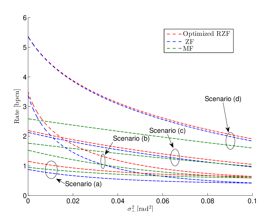
Fig. 6: C⁡(𝖲𝖨𝖭𝖱k)C(\mathsf{SINR}_{k}) of the different precoders in the GO setup for M=50,Mosc=5,q0=0.9M=50,M_{\mathrm{osc}}=5,q_{0}=0.9, and different σϕ2\sigma_{\mathrm{\phi}}^{{2}} values. The operating scenarios considered are the following: Scenario (a): SNR=0\mathrm{SNR}=0 dB, β=2\beta=2. Scenario (b): SNR=20\mathrm{SNR}=20 dB, β=2\beta=2. Scenario (c): SNR=0\mathrm{SNR}=0 dB, β=5\beta=5. Scenario (d): SNR=20\mathrm{SNR}=20dB, β=5\beta=5.

We compare C⁡(𝖲𝖨𝖭𝖱k)C(\mathsf{SINR}_{k}) of the considered precoders for different σϕ2\sigma_{\mathrm{\phi}}^{{2}} values and operating scenarios in Fig. 6. We set M=50,Mosc=5,M=50,M_{\mathrm{osc}}=5, and q0=0.9q_{0}=0.9 for all scenarios. In Scenario (a), we set β=2\beta=2 and SNR=0\mathrm{SNR}=0 dB. In this scenario, the performance of the MF precoder is consistently better than that of the ZF precoder, and approaches the performance of the optimized RZF precoder as σϕ2\sigma_{\mathrm{\phi}}^{{2}} increases. As the SNR is increased to 2020 dB in Scenario (b), the ZF precoder performs better than the MF precoder for low values of σϕ2\sigma_{\mathrm{\phi}}^{{2}}. But for large σφ2\sigma_{\mathrm{\varphi}}^{{2}} values, the order is reversed.

In Scenario (c), we set the SNR to 00 dB, and increase β\beta to 5, thereby reducing the interference. In this scenario, the ZF precoder is seen to perform better than the MF precoder, except when the phase noise is severe. Finally, in Scenario (d), the SNR is increased to 20 dB, and the ZF precoder significantly outperforms the MF precoder for all σφ2\sigma_{\mathrm{\varphi}}^{{2}} values considered. In summary, we conclude that the relative performance of the MF and ZF precoders depends on the operating scenario, which depends on the values of MoscM_{\mathrm{osc}}, MM, q0q_{0}, σφ2\sigma_{\mathrm{\varphi}}^{{2}}, SNR, and β\beta.

Refer to caption
Fig. 7: C⁡(𝖲𝖨𝖭𝖱k)C(\mathsf{SINR}_{k}) of the different precoders in the GO setup, where 1≤Mosc≤M,M/Mosc∈ℤ+1\leq M_{\mathrm{osc}}\leq M,M/M_{\mathrm{osc}}\in\mathbb{Z}^{+}, for M=50,β=2,q0=0.9M=50,\beta=2,q_{0}=0.9, σϕ=σφ=0.06∘\sigma_{\mathrm{\phi}}=\sigma_{\mathrm{\varphi}}=0.06^{\circ}, τ=Tc=0.25​ms\tau=T_{\mathrm{c}}=0.25~\textrm{ms} (10410^{4} symbol periods) [36], and different SNR values.

V-D Example Based on LTE Specifications

We analyze an example based on long-term evolution (LTE) system specifications [2, 36], where we account for practical values of TcT_{\mathrm{c}}, symbol time TsT_{\mathrm{s}}, bandwidth B​WBW, τ\tau, center frequency fcf_{\mathrm{c}}, doppler spread fdf_{\mathrm{d}}, σϕ\sigma_{\mathrm{\phi}}, and σφ\sigma_{\mathrm{\varphi}}. We choose Ts=0.032​μ​sT_{\mathrm{s}}=0.032\mu s, B​W=20BW=20 MHz, fc=2f_{\mathrm{c}}=2 GHz, and fd=1000f_{\mathrm{d}}=1000 Hz arising from a relative velocity of 500500 km/h between the BS and the UEs. Letting Tc=1/4​fdT_{\mathrm{c}}=1/4f_{\mathrm{d}}, the coherence time is Tc=0.25T_{\mathrm{c}}=0.25 ms. We also consider that the time elapsed between the training and the data transmission phase is equal to the coherence time of the channel, i.e., τ=Tc=0.25\tau=T_{\mathrm{c}}=0.25 ms [36, pg. 99].

Next, we compute σϕ2\sigma_{\mathrm{\phi}}^{{2}} and σφ2\sigma_{\mathrm{\varphi}}^{{2}} based on a Si CMOS oscillator technology in [37]. Specifically, we consider an oscillator, whose offset level at 9090 MHz is −156-156 dBc/Hz. This renders σϕ2=σφ2=10−6\sigma_{\mathrm{\phi}}^{{2}}=\sigma_{\mathrm{\varphi}}^{{2}}=10^{-6} rad2, or σϕ=σφ=0.06∘\sigma_{\mathrm{\phi}}=\sigma_{\mathrm{\varphi}}=0.06{}^{\circ} using [38, Eq. (4)], implying that high-quality oscillators are used at the BS and the UE. In Fig. 7, we plot the performance of the precoders versus MoscM_{\mathrm{osc}} for τ=Tc=0.25\tau=T_{\mathrm{c}}=0.25 ms (10410^{4} symbol periods), q0=0.9q_{0}=0.9, β=2\beta=2, and M=50M=50 for different SNR values. At SNR=20\mathrm{SNR}=20 dB, we observe that the performance of the RZF and ZF precoders decreases by around 0.30.3 bits per channel use (bpcu), as MoscM_{\mathrm{osc}} increases, and for Mosc>10M_{\mathrm{osc}}>10 oscillators at the BS, the additional degradation in performance becomes negligible. One the other hand, the degradation in the performance of the MF precoder is negligible for all values of MoscM_{\mathrm{osc}} considered. Furthermore, at SNR=0\mathrm{SNR}=0 dB, the performance degradation for all considered precoders is negligible as MoscM_{\mathrm{osc}} is increased from 1 to MM.

V-E Rate Comparisons for CO and DO Setups

We compare the performance of the CO setup with that of the DO setup by computing the achievable rate as C⁡(𝖲𝖨𝖭𝖱k)=min⁡{Rate​in​(20),Rate​in​(III-B)}C(\mathsf{SINR}_{k})=\min\{\mathrm{Rate~in~\eqref{eq:AchRate2}},\mathrm{Rate~in~\eqref{eq:AchRate3}}\}. We set q0=0.9q_{0}=0.9, σϕ=σφ=6∘\sigma_{\mathrm{\phi}}=\sigma_{\mathrm{\varphi}}=6^{\circ}, and τ=K=25\tau=K=25, and analyze the rate performance of the RZF and MF precoders for different values of β\beta in Figs. 8 and 9.

We first consider the optimized RZF precoder in Fig. 8. For SNR=40\mathrm{SNR}=40 dB, the performance of the CO setup is consistently better than that of the DO setup as the SINR used in (20) and (III-B) is large, and exclusively determines the achievable rate. In particular, when β\beta is small, the rate in (20) is a tighter upper bound, and the achievable rate is determined by the SINR term, which is relatively larger for the CO setup. As β\beta increases, the rate in (III-B) becomes a tighter upper bound, and the SINR term is much larger than the differential entropy term. Hence, the CO setup still performs better. Now, consider the low SNR scenario (SNR=0\mathrm{SNR}=0 dB). Here, once again, for small β\beta, the rate in (20) is a tighter upper bound than that in (III-B), and depends on the SINR alone. Therefore, the CO setup performs better. However, as β\beta increases, the rate in (III-B) becomes a tighter upper bound, and the differential entropy term becomes significant compared to the SINR term. In particular, the DO setup has a lower differential entropy rate as it is only impaired by the phase noise at the UE. Consequently, the DO setup performs better.

A similar performance order is observed in Fig. 9 for the MF precoder when SNR=0\mathrm{SNR}=0 dB. For SNR=40\mathrm{SNR}=40 dB and low β\beta values, as before, the achievable rate depends on the SINR alone as the rate in (20) is a tighter upper bound. However, as β\beta increases, the rate in (III-B) becomes a tighter upper bound. Unlike in the case of the RZF precoder, now the differential entropy term is significant compared to the SINR term in (III-B). This is because the SINR of the MF precoder is significantly lower than that of the RZF precoder. Moreover, the difference in the SINR for the CO and the DO setups is not as significant as when RZF precoding is used, since the interference power for the MF precoder is the same for both the setups (32). Therefore, the DO setup performs better than the CO setup.

Refer to caption
Fig. 8: C⁡(𝖲𝖨𝖭𝖱k)=min⁡{Rate​in​(20),Rate​in​(III-B)}C(\mathsf{SINR}_{k})=\min\{\mathrm{Rate~in~\eqref{eq:AchRate2}},\mathrm{Rate~in~\eqref{eq:AchRate3}}\} of the optimized RZF precoder for the CO and DO setups, where q0=0.9q_{0}=0.9, σϕ=σφ=6∘\sigma_{\mathrm{\phi}}=\sigma_{\mathrm{\varphi}}=6^{\circ}, and τ=K=25\tau=K=25.
Refer to caption
Fig. 9: C⁡(𝖲𝖨𝖭𝖱k)=min⁡{Rate​in​(20),Rate​in​(III-B)}C(\mathsf{SINR}_{k})=\min\{\mathrm{Rate~in~\eqref{eq:AchRate2}},\mathrm{Rate~in~\eqref{eq:AchRate3}}\} of the MF precoder for the CO and DO setups, where q0=0.9q_{0}=0.9, σϕ=σφ=6∘\sigma_{\mathrm{\phi}}=\sigma_{\mathrm{\varphi}}=6^{\circ}, and τ=K=25\tau=K=25.

VI Conclusions

In this work, we derived the effective SINR of the RZF, ZF, and MF precoders for the GO setup in the presence of phase noise. We showed that the effect of phase noise on the SINR can be expressed as an effective reduction in the CSI quality available at the BS. Importantly, the SINR performance of all considered precoders degrades as the number of oscillators, MoscM_{\mathrm{osc}}, increases. This is because as MoscM_{\mathrm{osc}} increases, the desired signal power decreases, and the interference power increases. However, for the MF precoder, the interference power is almost independent of the phase noise. Furthermore, we showed that the variance of the random phase variations caused by the BS oscillators reduces with increasing MoscM_{\mathrm{osc}}. By simulations, we demonstrated that the SINR approximations obtained are tight, and agree with those obtained from simulations with remarkable accuracy for interesting, and practical values of MM and KK.

We showed that the optimized RZF has superior SINR performance compared to the ZF and the MF precoders for all considered scenarios. Moreover, the ZF precoder performs better than the MF precoder when the CSI available at the BS is reliable, the phase noise at the BS is not severe, and β\beta is large. However, for low SNR, severe phase noise at the BS, and small β\beta, the MF performs better. Finally, we observed that for all considered precoders, the CO setup has a higher achievable rate than the DO setup when β\beta is small, while the DO setup outperforms the CO setup when the SNR at the UE is low and β\beta is large.

APPENDIX A

Important Results from Literature

Definition 1 (Stieltjes Transform [32, Section 2.2])

Let XX be a real-valued RV with distribution FF. The the Stieltjes transform m⁡(z)m(z) of FF, for z∈ℂz\in\mathbb{C} such that ℑ⁡{z}>0\Im\{z\}>0, is defined as

m⁡(z)=𝔼⁡[1X−z]=∫−∞∞1λ−z​𝑑F​(λ).\displaystyle m(z)=\mathbb{E}\left[\frac{1}{X-z}\right]=\int_{-\infty}^{\infty}\frac{1}{\lambda-z}dF(\lambda). (38)
Lemma 1

Stieltjes Transform of the Marchenko-Pastur Law [32, Eqs. (1.12, 2.43)]: Let 𝐇∈ℂK×M\mathbf{H}\in\mathbb{C}^{K\times M}, with entries that are zero-mean i.i.d. RVs with variance 1/M1/M. Then the empirical distribution of the eigenvalues of 𝐇H​𝐇\mathbf{H}^{\mathrm{H}}\mathbf{H} converges to the Marchenko-Pastur law almost surely as M,K→∞M,K\rightarrow\infty, with M/K=βM/K=\beta. Furthermore, the Stieltjes transform m⁡(z)m(z), with complex argument zz such that ℑ⁡{z}>0\Im\{z\}>0, of the Marchenko-Pastur density law is defined as

m⁡(z)=1−z​β−β±β2​z2−2​(β+1)​z​β+(1−β)22​z​β\displaystyle m(z)=\frac{1-z\beta-\beta\pm\sqrt{\beta^{2}z^{2}-2(\beta+1)z\beta+(1-\beta)^{2}}}{2z\beta} (39)
Lemma 2 (Matrix Inversion Lemma [33, Eq. (2.2)])

For an invertible matrix 𝐔∈ℂM×M\mathbf{U}\in\mathbb{C}^{M\times M}, 𝐡∈ℂM×1\mathbf{h}\in\mathbb{C}^{M\times 1}, and q∈ℂq\in\mathbb{C}, where 𝐔+q​𝐡𝐡H\mathbf{U}+q\mathbf{h}\mathbf{h}^{\mathrm{H}} is invertible,

𝐡H​(𝐔+q​𝐡𝐡H)−1=𝐡H​𝐔−11+q​𝐡H​𝐔−1​𝐡,\displaystyle\mathbf{h}^{\mathrm{H}}(\mathbf{U}+q\mathbf{h}\mathbf{h}^{\mathrm{H}})^{\scalebox{0.5}[1.0]{$-$}1}=\frac{\mathbf{h}^{\mathrm{H}}\mathbf{U}^{\scalebox{0.5}[1.0]{$-$}1}}{1+q\mathbf{h}^{\mathrm{H}}\mathbf{U}^{\scalebox{0.5}[1.0]{$-$}1}\mathbf{h}}, (40)

since 𝐡H​𝐔−1​(𝐔+q​𝐡𝐡H)=(1+q​𝐡H​𝐔−1​𝐡)​𝐡H\mathbf{h}^{\mathrm{H}}\mathbf{U}^{\scalebox{0.5}[1.0]{$-$}1}(\mathbf{U}+q\mathbf{h}\mathbf{h}^{\mathrm{H}})=(1+q\mathbf{h}^{\mathrm{H}}\mathbf{U}^{\scalebox{0.5}[1.0]{$-$}1}\mathbf{h})\mathbf{h}^{\mathrm{H}}.

Lemma 3 (Resolvent Identity [14, Lemma 2])

Given two invertible matrices 𝐔\mathbf{U} and 𝐕\mathbf{V} of size M×MM\times M,

𝐔−1−𝐕−1=−𝐔−1​(𝐔−𝐕)​𝐕−1\displaystyle\mathbf{U}^{\scalebox{0.5}[1.0]{$-$}1}-\mathbf{V}^{\scalebox{0.5}[1.0]{$-$}1}=-\mathbf{U}^{\scalebox{0.5}[1.0]{$-$}1}(\mathbf{U}-\mathbf{V})\mathbf{V}^{\scalebox{0.5}[1.0]{$-$}1} (41)

holds.

Lemma 4 (Trace Lemma [14, Lemma 4])

Let 𝐱,𝐰∼𝒞​𝒩​(0,1M​𝐈M)\mathbf{x},\mathbf{w}\sim{\mathcal{C}}{\mathcal{N}}(0,\frac{1}{M}\mathbf{I}_{M}) be mutually independent vectors of length MM, and also independent of 𝐀∈ℂM×M\mathbf{A}\in\mathbb{C}^{M\times M}, which has a uniformly bounded spectral norm for all MM. Then

𝐱H​𝐀𝐱−1M​tr​𝐀​⟶M→∞​0,𝐱H​𝐀𝐰​⟶M→∞​0.\displaystyle\mathbf{x}^{\mathrm{H}}\mathbf{A}\mathbf{x}-\frac{1}{M}\mathrm{tr}\mathbf{A}\overset{M\rightarrow\infty}{\longrightarrow}0,\mathbf{x}^{\mathrm{H}}\mathbf{A}\mathbf{w}\overset{M\rightarrow\infty}{\longrightarrow}0. (42)
Lemma 5

Let 𝐇∈ℂK×M\mathbf{H}\in\mathbb{C}^{K\times M}, M,K→∞M,K\rightarrow\infty with M/K=βM/K=\beta, whose entries are zero-mean i.i.d. Gaussian RVs with variance 1/M1/M, and define 𝐀≜1M​𝐇H​𝐇+α​𝐈M\mathbf{A}\triangleq\frac{1}{M}\mathbf{H}^{\mathrm{H}}\mathbf{H}+\alpha\mathbf{I}_{M}. Then

1M​tr​𝐀−1−m⁡(−α)⟶0,1M​tr​𝐀−2−m′​(−α)⟶0\displaystyle\frac{1}{M}{\mathrm{tr}\mathbf{A}^{\scalebox{0.5}[1.0]{$-$}1}}-m(-\alpha)\longrightarrow 0,\frac{1}{M}{\mathrm{tr}\mathbf{A}^{-2}}-m^{\prime}(-\alpha)\longrightarrow 0 (43)
Lemma 6 (Rank-1 Perturbation Lemma [33, Lemma 2.6])

Let ζ>0\zeta>0, 𝐔,and​𝐀∈ℂM×M\mathbf{U},~\textrm{and}~\mathbf{A}\in\mathbb{C}^{M\times M} with 𝐔\mathbf{U} being nonnegative Hermitian, 𝐡∈ℂM×1\mathbf{h}\in\mathbb{C}^{M\times 1}, and q∈ℝq\in\mathbb{R}. Then,

|tr​𝐀​[(𝐔+ζ​𝐈M+q​𝐡𝐡H)−1−(𝐔+ζ​𝐈M)−1]|≤‖𝐀‖ζ.\displaystyle|\mathrm{tr}\mathbf{A}\left[(\mathbf{U}+\zeta\mathbf{I}_{M}+q\mathbf{h}\mathbf{h}^{\mathrm{H}})^{\scalebox{0.5}[1.0]{$-$}1}-(\mathbf{U}+\zeta\mathbf{I}_{M})^{\scalebox{0.5}[1.0]{$-$}1}\right]|\leq\frac{||\mathbf{A}||}{\zeta}. (44)
Lemma 7 ( [14, Lemma 6])

Let 𝐔,𝐀∈ℂM×M\mathbf{U},\mathbf{A}\in\mathbb{C}^{M\times M} with 𝐔\mathbf{U} being nonnegative Hermitian, 𝐡∈ℂM\mathbf{h}\in\mathbb{C}^{M} and q∈ℝq\in\mathbb{R}, then,

1M​tr​𝐀𝐔−1−1M​tr​𝐀​(𝐔+q​𝐡𝐡H)−1​⟶M→∞​0\displaystyle\frac{1}{M}{\mathrm{tr}\mathbf{A}\mathbf{U}^{\scalebox{0.5}[1.0]{$-$}1}}-\frac{1}{M}{\mathrm{tr}\mathbf{A}(\mathbf{U}+q\mathbf{h}\mathbf{h}^{\mathrm{H}})^{\scalebox{0.5}[1.0]{$-$}1}}\overset{M\rightarrow\infty}{\longrightarrow}0 (45)
Lemma 8 ( [14, Lemma 7])

Consider 𝐔,𝐀∈ℂM×M\mathbf{U},\mathbf{A}\in\mathbb{C}^{M\times M} with uniformly bounded spectral norms for all MM with 𝐀\mathbf{A} being invertible. Furthermore, let 𝐱,𝐰∼𝒞​𝒩​(0,1M​𝐈M)\mathbf{x},\mathbf{w}\sim{\mathcal{C}}{\mathcal{N}}(0,\frac{1}{M}\mathbf{I}_{M}) be mutually independent vectors of length MM, and also independent of 𝐔,𝐀\mathbf{U}_{,}\mathbf{A}. Define q0,q1,q2∈ℝ+q_{0},q_{1},q_{2}\in\mathbb{R}^{+} such that q0​q1=q22q_{0}q_{1}=q_{2}^{2}, q0+q1=1q_{0}+q_{1}=1 and t1≜1M​tr​𝐀−1,t2≜1M​tr​𝐔𝐀−1t_{1}\triangleq\frac{1}{M}\mathrm{tr}\mathbf{A}^{\scalebox{0.5}[1.0]{$-$}1},t_{2}\triangleq\frac{1}{M}\mathrm{tr}\mathbf{U}\mathbf{A}^{\scalebox{0.5}[1.0]{$-$}1}. Then,

𝐱H​𝐔​(𝐀+q0​𝐱𝐱H+q1​𝐰𝐰H+q2​𝐱𝐰H+q2​𝐰𝐱H)−1​𝐱\displaystyle\mathbf{x}^{\mathrm{H}}\mathbf{U}\left(\mathbf{A}+q_{0}\mathbf{x}\mathbf{x}^{\mathrm{H}}+q_{1}\mathbf{w}\mathbf{w}^{\mathrm{H}}+q_{2}\mathbf{x}\mathbf{w}^{\mathrm{H}}+q_{2}\mathbf{w}\mathbf{x}^{\mathrm{H}}\right)^{\scalebox{0.5}[1.0]{$-$}1}\mathbf{x}
−t2​(1+q1​t1)1+t1​⟶M→∞​0\displaystyle-\frac{t_{2}(1+q_{1}t_{1})}{1+t_{1}}\overset{M\rightarrow\infty}{\longrightarrow}0 (46)
𝐰H​𝐔​(𝐀+q0​𝐱𝐱H+q1​𝐰𝐰H+q2​𝐱𝐰H+q2​𝐰𝐱H)−1​𝐰\displaystyle\mathbf{w}^{\mathrm{H}}\mathbf{U}\left(\mathbf{A}+q_{0}\mathbf{x}\mathbf{x}^{\mathrm{H}}+q_{1}\mathbf{w}\mathbf{w}^{\mathrm{H}}+q_{2}\mathbf{x}\mathbf{w}^{\mathrm{H}}+q_{2}\mathbf{w}\mathbf{x}^{\mathrm{H}}\right)^{\scalebox{0.5}[1.0]{$-$}1}\mathbf{w}
−t2​(1+q0​t1)1+t1​⟶M→∞​0\displaystyle-\frac{t_{2}(1+q_{0}t_{1})}{1+t_{1}}\overset{M\rightarrow\infty}{\longrightarrow}0 (47)
𝐱H​𝐔​(𝐀+q0​𝐱𝐱H+q1​𝐰𝐰H+q2​𝐱𝐰H+q2​𝐰𝐱H)−1​𝐰\displaystyle\mathbf{x}^{\mathrm{H}}\mathbf{U}\left(\mathbf{A}+q_{0}\mathbf{x}\mathbf{x}^{\mathrm{H}}+q_{1}\mathbf{w}\mathbf{w}^{\mathrm{H}}+q_{2}\mathbf{x}\mathbf{w}^{\mathrm{H}}+q_{2}\mathbf{w}\mathbf{x}^{\mathrm{H}}\right)^{\scalebox{0.5}[1.0]{$-$}1}\mathbf{w}
−−q2​t1​t21+t1​⟶M→∞​0\displaystyle-\frac{-q_{2}t_{1}t_{2}}{1+t_{1}}\overset{M\rightarrow\infty}{\longrightarrow}0 (48)
𝐰H​𝐔​(𝐀+q0​𝐱𝐱H+q1​𝐰𝐰H+q2​𝐱𝐰H+q2​𝐰𝐱H)−1​𝐱\displaystyle\mathbf{w}^{\mathrm{H}}\mathbf{U}\left(\mathbf{A}+q_{0}\mathbf{x}\mathbf{x}^{\mathrm{H}}+q_{1}\mathbf{w}\mathbf{w}^{\mathrm{H}}+q_{2}\mathbf{x}\mathbf{w}^{\mathrm{H}}+q_{2}\mathbf{w}\mathbf{x}^{\mathrm{H}}\right)^{\scalebox{0.5}[1.0]{$-$}1}\mathbf{x}
−−q2​t1​t21+t1​⟶M→∞​0.\displaystyle-\frac{-q_{2}t_{1}t_{2}}{1+t_{1}}\overset{M\rightarrow\infty}{\longrightarrow}0. (49)
Lemma 9

Let 𝐔,𝐕∈ℂM×M\mathbf{U},\mathbf{V}\in\mathbb{C}^{M\times M} be freely independent random matrices [34, Page 207] with uniformly bounded spectral norm for all MM. Further, let all the moments of the entries of 𝐔,𝐕\mathbf{U},\mathbf{V} be finite. Then,

1M​tr​𝐔𝐕−1M​tr​𝐔​1M​tr​𝐕​⟶M→∞​0.\displaystyle\frac{1}{M}\mathrm{tr}\mathbf{U}\mathbf{V}-\frac{1}{M}\mathrm{tr}\mathbf{U}\frac{1}{M}\mathrm{tr}\mathbf{V}\overset{M\rightarrow\infty}{\longrightarrow}0. (50)

APPENDIX B

Extensions to Existing Lemmas in [14]

First, we provide Lemma 10, which is an extension to Lemma 8 [14, Lemma 7]. Lemma 10 is then used to the derive the effective SINR in (24).

Lemma 10 (Extensions to [14, Lemma 7])

Consider 𝐔\mathbf{U}, 𝐀\mathbf{A}, 𝐍∈ℂM×M\mathbf{N}\in\mathbb{C}^{M\times M} with uniformly bounded spectral norms for all MM, such that 𝐀\mathbf{A} is invertible, and 𝐍\mathbf{N} is unitary, 𝐍𝐍H=𝐈M\mathbf{N}\mathbf{N}^{\mathrm{H}}=\mathbf{I}_{M}. Furthermore, assume that 𝐍\mathbf{N} is freely independent of 𝐔,𝐀\mathbf{U},\mathbf{A} [34, Page 207]. Let 𝐱,𝐰∼𝒞​𝒩​(0,1M​𝐈M)\mathbf{x},\mathbf{w}\sim{\mathcal{C}}{\mathcal{N}}(0,\frac{1}{M}\mathbf{I}_{M}) be mutually independent vectors of length MM, and also independent of 𝐔,𝐀\mathbf{U}_{,}\mathbf{A}. Define q0,q1,q2∈ℝ+q_{0},q_{1},q_{2}\in\mathbb{R}^{+} such that q0​q1=q22q_{0}q_{1}=q_{2}^{2}, q0+q1=1q_{0}+q_{1}=1 and t1≜1M​tr​𝐀−1,t2≜1M​tr​𝐔𝐀−1t_{1}\triangleq\frac{1}{M}\mathrm{tr}\mathbf{A}^{\scalebox{0.5}[1.0]{$-$}1},t_{2}\triangleq\frac{1}{M}\mathrm{tr}\mathbf{U}\mathbf{A}^{\scalebox{0.5}[1.0]{$-$}1}. Then,

𝐱H​𝐍𝐔​(𝐀+q0​𝐱𝐱H+q1​𝐰𝐰H+q2​𝐱𝐰H+q2​𝐰𝐱H)−1​𝐍H​𝐱\displaystyle\mathbf{x}^{\mathrm{H}}\mathbf{N}\mathbf{U}\left(\mathbf{A}+q_{0}\mathbf{x}\mathbf{x}^{\mathrm{H}}+q_{1}\mathbf{w}\mathbf{w}^{\mathrm{H}}+q_{2}\mathbf{x}\mathbf{w}^{\mathrm{H}}+q_{2}\mathbf{w}\mathbf{x}^{\mathrm{H}}\right)^{\scalebox{0.5}[1.0]{$-$}1}\mathbf{N}^{\mathrm{H}}\mathbf{x}
−(t2−q0​t1​t21+t1​|tr​{𝐍}M|2)​⟶M→∞​0\displaystyle-\left(t_{2}-\frac{q_{0}t_{1}t_{2}}{1+t_{1}}\left|\frac{\mathrm{tr}\left\{\mathbf{N}\right\}}{M}\right|^{2}\right)\overset{M\rightarrow\infty}{\longrightarrow}0 (51)
𝐱H​𝐔​(𝐀+q0​𝐱𝐱H+q1​𝐰𝐰H+q2​𝐱𝐰H+q2​𝐰𝐱H)−1​𝐍H​𝐱\displaystyle\mathbf{x}^{\mathrm{H}}\mathbf{U}\left(\mathbf{A}+q_{0}\mathbf{x}\mathbf{x}^{\mathrm{H}}+q_{1}\mathbf{w}\mathbf{w}^{\mathrm{H}}+q_{2}\mathbf{x}\mathbf{w}^{\mathrm{H}}+q_{2}\mathbf{w}\mathbf{x}^{\mathrm{H}}\right)^{\scalebox{0.5}[1.0]{$-$}1}\mathbf{N}^{\mathrm{H}}\mathbf{x}
−t2​(1+q1​t1)1+t1​tr​{𝐍H}M​⟶M→∞​0\displaystyle-\frac{t_{2}(1+q_{1}t_{1})}{1+t_{1}}\frac{\mathrm{tr}\left\{\mathbf{N}^{\mathrm{H}}\right\}}{M}\overset{M\rightarrow\infty}{\longrightarrow}0 (52)
𝐰H​𝐔​(𝐀+q0​𝐱𝐱H+q1​𝐰𝐰H+q2​𝐱𝐰H+q2​𝐰𝐱H)−1​𝐍H​𝐱\displaystyle\mathbf{w}^{\mathrm{H}}\mathbf{U}\left(\mathbf{A}+q_{0}\mathbf{x}\mathbf{x}^{\mathrm{H}}+q_{1}\mathbf{w}\mathbf{w}^{\mathrm{H}}+q_{2}\mathbf{x}\mathbf{w}^{\mathrm{H}}+q_{2}\mathbf{w}\mathbf{x}^{\mathrm{H}}\right)^{\scalebox{0.5}[1.0]{$-$}1}\mathbf{N}^{\mathrm{H}}\mathbf{x}
−−q2​t1​t21+t1​tr​{𝐍H}M​⟶M→∞​0\displaystyle-\frac{-q_{2}t_{1}t_{2}}{1+t_{1}}\frac{\mathrm{tr}\left\{\mathbf{N}^{\mathrm{H}}\right\}}{M}\overset{M\rightarrow\infty}{\longrightarrow}0 (53)
Proof:

Since 𝐍\mathbf{N} is freely independent of 𝐔,𝐀\mathbf{U},\mathbf{A}, from Lemma 9 we have

1M​tr​𝐍𝐀−1−1M​tr​𝐍​1M​tr​𝐀−1⏟≜t1​⟶M→∞​0\displaystyle\frac{1}{M}\mathrm{tr}\mathbf{N}\mathbf{A}^{\scalebox{0.5}[1.0]{$-$}1}-\frac{1}{M}\mathrm{tr}\mathbf{N}\underbrace{\frac{1}{M}\mathrm{tr}\mathbf{A}^{\scalebox{0.5}[1.0]{$-$}1}}_{\triangleq t_{1}}\overset{M\rightarrow\infty}{\longrightarrow}0 (54)
1M​tr​𝐍𝐔𝐀−1−1M​tr​𝐍​1M​tr​𝐔𝐀−1⏟≜t2​⟶M→∞​0.\displaystyle\frac{1}{M}\mathrm{tr}\mathbf{N}\mathbf{U}\mathbf{A}^{\scalebox{0.5}[1.0]{$-$}1}-\frac{1}{M}\mathrm{tr}\mathbf{N}\underbrace{\frac{1}{M}\mathrm{tr}\mathbf{U}\mathbf{A}^{\scalebox{0.5}[1.0]{$-$}1}}_{\triangleq t_{2}}\overset{M\rightarrow\infty}{\longrightarrow}0. (55)

Furthermore,

𝐱H​𝐍𝐔𝐕𝐱−tr​𝐍M​t2​(1+q1​t1)1+t1​⟶M→∞​0\displaystyle\mathbf{x}^{\mathrm{H}}\mathbf{N}\mathbf{U}\mathbf{V}\mathbf{x}-\frac{\mathrm{tr}\mathbf{N}}{M}\frac{t_{2}(1+q_{1}t_{1})}{1+t_{1}}\overset{M\rightarrow\infty}{\longrightarrow}0 (56)
𝐱H​𝐀−1​𝐍H​𝐱−tr​𝐍HM​t1​⟶M→∞​0\displaystyle\mathbf{x}^{\mathrm{H}}\mathbf{A}^{\scalebox{0.5}[1.0]{$-$}1}\mathbf{N}^{\mathrm{H}}\mathbf{x}-\frac{\mathrm{tr}\mathbf{N}^{\mathrm{H}}}{M}t_{1}\overset{M\rightarrow\infty}{\longrightarrow}0 (57)
𝐱H​𝐔𝐀−1​𝐍H​𝐱−tr​𝐍HM​t2​⟶M→∞​0\displaystyle\mathbf{x}^{\mathrm{H}}\mathbf{U}\mathbf{A}^{\scalebox{0.5}[1.0]{$-$}1}\mathbf{N}^{\mathrm{H}}\mathbf{x}-\frac{\mathrm{tr}\mathbf{N}^{\mathrm{H}}}{M}t_{2}\overset{M\rightarrow\infty}{\longrightarrow}0 (58)
𝐱H​𝐍𝐔𝐕𝐰−−q2​t1​t21+t1​tr​𝐍M​⟶M→∞​0\displaystyle\mathbf{x}^{\mathrm{H}}\mathbf{N}\mathbf{U}\mathbf{V}\mathbf{w}-\frac{-q_{2}t_{1}t_{2}}{1+t_{1}}\frac{\mathrm{tr}\mathbf{N}}{M}\overset{M\rightarrow\infty}{\longrightarrow}0 (59)
𝐱H​𝐍𝐔𝐀−1​𝐍H​𝐱−t2​⟶M→∞​0\displaystyle\mathbf{x}^{\mathrm{H}}\mathbf{N}\mathbf{U}\mathbf{A}^{\scalebox{0.5}[1.0]{$-$}1}\mathbf{N}^{\mathrm{H}}\mathbf{x}-t_{2}\overset{M\rightarrow\infty}{\longrightarrow}0 (60)
𝐰H​𝐀−1​𝐍H​𝐱​⟶M→∞​0.\displaystyle\mathbf{w}^{\mathrm{H}}\mathbf{A}^{\scalebox{0.5}[1.0]{$-$}1}\mathbf{N}^{\mathrm{H}}\mathbf{x}\overset{M\rightarrow\infty}{\longrightarrow}0. (61)

In order to obtain (56) and (59), the result in (55) along with Lemma 8 is applied. The results in (57), (58), (60), and (61) are obtained by using (54), (55), and Lemma 4. Now, define 𝐕≜(𝐀+q0​𝐱𝐱H+q1​𝐰𝐰H+q2​𝐰𝐱H+q2​𝐱𝐰H)−1,\mathbf{V}\triangleq(\mathbf{A}+q_{0}\mathbf{x}\mathbf{x}^{\mathrm{H}}+q_{1}\mathbf{w}\mathbf{w}^{\mathrm{H}}+q_{2}\mathbf{w}\mathbf{x}^{\mathrm{H}}+q_{2}\mathbf{x}\mathbf{w}^{\mathrm{H}})^{\scalebox{0.5}[1.0]{$-$}1}, then

𝐱H​𝐍𝐔𝐕𝐍H​𝐱\displaystyle\mathbf{x}^{\mathrm{H}}\mathbf{N}\mathbf{U}\mathbf{V}\mathbf{N}^{\mathrm{H}}\mathbf{x}
=𝐱H​𝐍𝐔𝐀−1​𝐍H​𝐱−𝐱H​𝐍𝐔​(𝐕−1−𝐀)​𝐀−1​𝐍H​𝐱\displaystyle=\mathbf{x}^{\mathrm{H}}\mathbf{N}\mathbf{U}\mathbf{A}^{\scalebox{0.5}[1.0]{$-$}1}\mathbf{N}^{\mathrm{H}}\mathbf{x}-\mathbf{x}^{\mathrm{H}}\mathbf{N}\mathbf{U}(\mathbf{V}^{\scalebox{0.5}[1.0]{$-$}1}-\mathbf{A})\mathbf{A}^{\scalebox{0.5}[1.0]{$-$}1}\mathbf{N}^{\mathrm{H}}\mathbf{x} (62)
=𝐱H​𝐍𝐔𝐀−1​𝐍H​𝐱−𝐱H​𝐍𝐔𝐕​(q0​𝐱𝐱H+q1​𝐰𝐰H+q2​𝐰𝐱HCLOSE\displaystyle=\mathbf{x}^{\mathrm{H}}\mathbf{N}\mathbf{U}\mathbf{A}^{\scalebox{0.5}[1.0]{$-$}1}\mathbf{N}^{\mathrm{H}}\mathbf{x}-\mathbf{x}^{\mathrm{H}}\mathbf{N}\mathbf{U}\mathbf{V}\left(q_{0}\mathbf{x}\mathbf{x}^{\mathrm{H}}+q_{1}\mathbf{w}\mathbf{w}^{\mathrm{H}}+q_{2}\mathbf{w}\mathbf{x}^{\mathrm{H}}\right.
OPEN+q2​𝐱𝐰H)​𝐀−1​𝐍H​𝐱\displaystyle\left.~+q_{2}\mathbf{x}\mathbf{w}^{\mathrm{H}}\right)\mathbf{A}^{\scalebox{0.5}[1.0]{$-$}1}\mathbf{N}^{\mathrm{H}}\mathbf{x} (63)
=−q0​𝐱H​𝐍𝐔𝐕𝐱𝐱H​𝐀−1​𝐍H​𝐱−q1​𝐱H​𝐍𝐔𝐕𝐰𝐰H​𝐀−1​𝐍H​𝐱\displaystyle=-q_{0}\mathbf{x}^{\mathrm{H}}\mathbf{N}\mathbf{U}\mathbf{V}\mathbf{x}\mathbf{x}^{\mathrm{H}}\mathbf{A}^{\scalebox{0.5}[1.0]{$-$}1}\mathbf{N}^{\mathrm{H}}\mathbf{x}-q_{1}\mathbf{x}^{\mathrm{H}}\mathbf{N}\mathbf{U}\mathbf{V}\mathbf{w}\mathbf{w}^{\mathrm{H}}\mathbf{A}^{\scalebox{0.5}[1.0]{$-$}1}\mathbf{N}^{\mathrm{H}}\mathbf{x}
−q2​𝐱H​𝐍𝐔𝐕𝐰𝐱H​𝐀−1​𝐍H​𝐱−q2​𝐱H​𝐍𝐔𝐕𝐱𝐰H​𝐀−1​𝐍H​𝐱\displaystyle~-q_{2}\mathbf{x}^{\mathrm{H}}\mathbf{N}\mathbf{U}\mathbf{V}\mathbf{w}\mathbf{x}^{\mathrm{H}}\mathbf{A}^{\scalebox{0.5}[1.0]{$-$}1}\mathbf{N}^{\mathrm{H}}\mathbf{x}-q_{2}\mathbf{x}^{\mathrm{H}}\mathbf{N}\mathbf{U}\mathbf{V}\mathbf{x}\mathbf{w}^{\mathrm{H}}\mathbf{A}^{\scalebox{0.5}[1.0]{$-$}1}\mathbf{N}^{\mathrm{H}}\mathbf{x} (64)
=t2−q0​t1​t2​(1+q1​t1)1+t1​|tr​{𝐍}M|2+q22​t12​t21+t1​|tr​{𝐍}M|2\displaystyle=t_{2}-\frac{q_{0}t_{1}t_{2}(1+q_{1}t_{1})}{1+t_{1}}\left|\frac{\mathrm{tr}\left\{\mathbf{N}\right\}}{M}\right|^{2}+\frac{q_{2}^{2}t_{1}^{2}t_{2}}{1+t_{1}}\left|\frac{\mathrm{tr}\left\{\mathbf{N}\right\}}{M}\right|^{2} (65)
=t2−q0​t1​t21+t1​|tr​{𝐍}M|2.\displaystyle=t_{2}-\frac{q_{0}t_{1}t_{2}}{1+t_{1}}\left|\frac{\mathrm{tr}\left\{\mathbf{N}\right\}}{M}\right|^{2}. (66)

In (62), the resolvent identity in Lemma 3 is used. Upon simplifying (64) by using (56)-(61), the expression in (65) is obtained, which is further simplified to the desired result in (66) using the fact that q0​q1=q22q_{0}q_{1}=q_{2}^{2}.

Consider the term 𝐱H​𝐔𝐕𝐍H​𝐱\mathbf{x}^{\mathrm{H}}\mathbf{U}\mathbf{V}\mathbf{N}^{\mathrm{H}}\mathbf{x}, which is written as

𝐱H​𝐔𝐕𝐍H​𝐱\displaystyle\mathbf{x}^{\mathrm{H}}\mathbf{U}\mathbf{V}\mathbf{N}^{\mathrm{H}}\mathbf{x}
=𝐱H​𝐔𝐀−1​𝐍H​𝐱−q0​𝐱H​𝐔𝐕𝐱𝐱H​𝐀−1​𝐍H​𝐱\displaystyle=\mathbf{x}^{\mathrm{H}}\mathbf{U}\mathbf{A}^{\scalebox{0.5}[1.0]{$-$}1}\mathbf{N}^{\mathrm{H}}\mathbf{x}-q_{0}\mathbf{x}^{\mathrm{H}}\mathbf{U}\mathbf{V}\mathbf{x}\mathbf{x}^{\mathrm{H}}\mathbf{A}^{\scalebox{0.5}[1.0]{$-$}1}\mathbf{N}^{\mathrm{H}}\mathbf{x}
−q1​𝐱H​𝐔𝐕𝐰𝐰H​𝐀−1​𝐍H​𝐱−q2​𝐱H​𝐔𝐕𝐰𝐱H​𝐀−1​𝐍H​𝐱\displaystyle~-q_{1}\mathbf{x}^{\mathrm{H}}\mathbf{U}\mathbf{V}\mathbf{w}\mathbf{w}^{\mathrm{H}}\mathbf{A}^{\scalebox{0.5}[1.0]{$-$}1}\mathbf{N}^{\mathrm{H}}\mathbf{x}-q_{2}\mathbf{x}^{\mathrm{H}}\mathbf{U}\mathbf{V}\mathbf{w}\mathbf{x}^{\mathrm{H}}\mathbf{A}^{\scalebox{0.5}[1.0]{$-$}1}\mathbf{N}^{\mathrm{H}}\mathbf{x}
−q2​𝐱H​𝐔𝐕𝐱𝐰H​𝐀−1​𝐍H​𝐱\displaystyle~-q_{2}\mathbf{x}^{\mathrm{H}}\mathbf{U}\mathbf{V}\mathbf{x}\mathbf{w}^{\mathrm{H}}\mathbf{A}^{\scalebox{0.5}[1.0]{$-$}1}\mathbf{N}^{\mathrm{H}}\mathbf{x} (67)
=𝐱H​𝐔𝐀−1​𝐍H​𝐱−q0​𝐱H​𝐔𝐕𝐱𝐱H​𝐀−1​𝐍H​𝐱\displaystyle=\mathbf{x}^{\mathrm{H}}\mathbf{U}\mathbf{A}^{\scalebox{0.5}[1.0]{$-$}1}\mathbf{N}^{\mathrm{H}}\mathbf{x}-q_{0}\mathbf{x}^{\mathrm{H}}\mathbf{U}\mathbf{V}\mathbf{x}\mathbf{x}^{\mathrm{H}}\mathbf{A}^{\scalebox{0.5}[1.0]{$-$}1}\mathbf{N}^{\mathrm{H}}\mathbf{x}
−q2​𝐱H​𝐔𝐕𝐰𝐱H​𝐀−1​𝐍H​𝐱\displaystyle~-q_{2}\mathbf{x}^{\mathrm{H}}\mathbf{U}\mathbf{V}\mathbf{w}\mathbf{x}^{\mathrm{H}}\mathbf{A}^{\scalebox{0.5}[1.0]{$-$}1}\mathbf{N}^{\mathrm{H}}\mathbf{x} (68)
=(t2−q0​t1​t2​(1+q1​t1)1+t1+q22​t12​t21+t1)​tr​{𝐍H}M\displaystyle=\left(t_{2}-\frac{q_{0}t_{1}t_{2}(1+q_{1}t_{1})}{1+t_{1}}+\frac{q_{2}^{2}t_{1}^{2}t_{2}}{1+t_{1}}\right)\frac{\mathrm{tr}\left\{\mathbf{N}^{\mathrm{H}}\right\}}{M} (69)
=t2​(1+q1​t1)1+t1​tr​{𝐍H}M\displaystyle=\frac{t_{2}(1+q_{1}t_{1})}{1+t_{1}}\frac{\mathrm{tr}\left\{\mathbf{N}^{\mathrm{H}}\right\}}{M} (70)

In (67), Lemma 3 is applied, and (68) is reduced to (69) using the result in (61). Applying Lemma 8, along with the results in (57) and (58), the expression in (69) is obtained. Then, using the fact that q0​q1=q22q_{0}q_{1}=q_{2}^{2}, (69) reduces to the desired result in (70).

Finally, consider the term 𝐰H​𝐔𝐕𝐍H​𝐱\mathbf{w}^{\mathrm{H}}\mathbf{U}\mathbf{V}\mathbf{N}^{\mathrm{H}}\mathbf{x}, which reads as

𝐰H​𝐔𝐕𝐍H​𝐱\displaystyle\mathbf{w}^{\mathrm{H}}\mathbf{U}\mathbf{V}\mathbf{N}^{\mathrm{H}}\mathbf{x}
=𝐰H​𝐔𝐀−1​𝐍H​𝐱−q0​𝐰H​𝐔𝐕𝐱𝐱H​𝐀−1​𝐍H​𝐱\displaystyle=\mathbf{w}^{\mathrm{H}}\mathbf{U}\mathbf{A}^{\scalebox{0.5}[1.0]{$-$}1}\mathbf{N}^{\mathrm{H}}\mathbf{x}-q_{0}\mathbf{w}^{\mathrm{H}}\mathbf{U}\mathbf{V}\mathbf{x}\mathbf{x}^{\mathrm{H}}\mathbf{A}^{\scalebox{0.5}[1.0]{$-$}1}\mathbf{N}^{\mathrm{H}}\mathbf{x}
−q1​𝐰H​𝐔𝐕𝐰𝐰H​𝐀−1​𝐍H​𝐱−q2​𝐰H​𝐔𝐕𝐰𝐱H​𝐀−1​𝐍H​𝐱\displaystyle~-q_{1}\mathbf{w}^{\mathrm{H}}\mathbf{U}\mathbf{V}\mathbf{w}\mathbf{w}^{\mathrm{H}}\mathbf{A}^{\scalebox{0.5}[1.0]{$-$}1}\mathbf{N}^{\mathrm{H}}\mathbf{x}-q_{2}\mathbf{w}^{\mathrm{H}}\mathbf{U}\mathbf{V}\mathbf{w}\mathbf{x}^{\mathrm{H}}\mathbf{A}^{\scalebox{0.5}[1.0]{$-$}1}\mathbf{N}^{\mathrm{H}}\mathbf{x}
−q2​𝐰H​𝐔𝐕𝐱𝐰H​𝐀−1​𝐍H​𝐱\displaystyle~-q_{2}\mathbf{w}^{\mathrm{H}}\mathbf{U}\mathbf{V}\mathbf{x}\mathbf{w}^{\mathrm{H}}\mathbf{A}^{\scalebox{0.5}[1.0]{$-$}1}\mathbf{N}^{\mathrm{H}}\mathbf{x} (71)
=−q0​𝐰H​𝐔𝐕𝐱𝐱H​𝐀−1​𝐍H​𝐱−q2​𝐰H​𝐔𝐕𝐰𝐱H​𝐀−1​𝐍H​𝐱\displaystyle=-q_{0}\mathbf{w}^{\mathrm{H}}\mathbf{U}\mathbf{V}\mathbf{x}\mathbf{x}^{\mathrm{H}}\mathbf{A}^{\scalebox{0.5}[1.0]{$-$}1}\mathbf{N}^{\mathrm{H}}\mathbf{x}-q_{2}\mathbf{w}^{\mathrm{H}}\mathbf{U}\mathbf{V}\mathbf{w}\mathbf{x}^{\mathrm{H}}\mathbf{A}^{\scalebox{0.5}[1.0]{$-$}1}\mathbf{N}^{\mathrm{H}}\mathbf{x} (72)
=(q0​q2​t12​t21+t1−q2​t1​t2​(1+q0​t1)1+t1)​tr​{𝐍H}M\displaystyle=\left(\frac{q_{0}q_{2}t_{1}^{2}t_{2}}{1+t_{1}}-\frac{q_{2}t_{1}t_{2}(1+q_{0}t_{1})}{1+t_{1}}\right)\frac{\mathrm{tr}\left\{\mathbf{N}^{\mathrm{H}}\right\}}{M} (73)
=−q2​t1​t21+t1​tr​{𝐍H}M.\displaystyle=-\frac{q_{2}t_{1}t_{2}}{1+t_{1}}\frac{\mathrm{tr}\left\{\mathbf{N}^{\mathrm{H}}\right\}}{M}. (74)

The resolvent identity in Lemma 3 is applied to obtain (71), which is reduced to (72) using (61). Furthermore, Lemmas 4, 8, and the result in (57) are used to simplify (73) to (74). ∎

Appendix C

Proof of Theorem 1

The evaluation of the SINR in (24) involves computing the following terms: (i) the normalization constant ξ\xi, (ii) the signal term Isig\mathrm{I}_{\mathrm{sig}}, and (iii) the interference power ∥𝐈int∥2{\lVert\boldsymbol{\mathrm{I}_{\mathrm{}}}_{\mathrm{int}}\rVert}^{2}. In the sequel, we derive the three terms of interest. Also, when deriving the signal term Isig\mathrm{I}_{\mathrm{sig}}, we prove Proposition 1.

VI-A Derivation of ξ\xi

First, we define 𝝌0≜𝐇^0H​𝐇^0M+α​𝐈M\boldsymbol{\chi}_{0}\triangleq\frac{\hat{\mathbf{H}}_{0}^{\mathrm{H}}\hat{\mathbf{H}}_{0}}{M}+\alpha\mathbf{I}_{M}, and denote by 𝝌0,−k\boldsymbol{\chi}_{0,\scalebox{0.5}[1.0]{$-$}k} the matrix obtained upon removing the kkth column of 𝝌0\boldsymbol{\chi}_{0}. The RZF precoder 𝐆0\mathbf{G}_{0} in (7) satisfies the power constraint tr⁡(𝐆0H​𝐆0)=1\mathrm{tr}\left(\mathbf{G}_{0}^{\mathrm{H}}\mathbf{G}_{0}\right)=1 implying that

ξ2​tr​{𝐏​𝐇^0​(𝐇^0H​𝐇^0+M​α​𝐈M)−2​𝐇^0H}=1\displaystyle\xi^{2}\mathrm{tr}\left\{\mathbf{P}\hat{\mathbf{H}}_{0}\left(\hat{\mathbf{H}}_{0}^{\mathrm{H}}\hat{\mathbf{H}}_{0}+M\alpha\mathbf{I}_{M}\right)^{\scalebox{0.5}[1.0]{$-$}2}\hat{\mathbf{H}}_{0}^{\mathrm{H}}\right\}=1 (75)
ξ2​∑k=1Kpk​𝐡^0,kT​(𝐇^0,−kH​𝐇^0,−k+M​α​𝐈M+𝐡^0,k∗​𝐡^0,kT)−2​𝐡^0,k∗=1\displaystyle\xi^{2}{\sum_{k=1}^{K}}p_{k}\hat{\mathbf{h}}_{0,k}^{\mathrm{T}}\left(\hat{\mathbf{H}}_{0,\scalebox{0.5}[1.0]{$-$}k}^{\mathrm{H}}\hat{\mathbf{H}}_{0,\scalebox{0.5}[1.0]{$-$}k}+M\alpha\mathbf{I}_{M}+\hat{\mathbf{h}}_{0,k}^{*}\hat{\mathbf{h}}_{0,k}^{\mathrm{T}}\right)^{\scalebox{0.5}[1.0]{$-$}2}\hat{\mathbf{h}}_{0,k}^{*}=1

The expression in (75) is rewritten by applying Lemma 2 twice as

1M​ξ2​∑k=1K1M​pk​𝐡^0,kT​𝝌0,−k−2​𝐡^0,k∗(1+1M​𝐡^0,kT​𝝌0,−k−1​𝐡^0,k∗)2=1\displaystyle\frac{1}{M}\xi^{2}{\sum_{k=1}^{K}}\frac{\frac{1}{M}p_{k}\hat{\mathbf{h}}_{0,k}^{\mathrm{T}}\boldsymbol{\chi}_{0,\scalebox{0.5}[1.0]{$-$}k}^{\scalebox{0.5}[1.0]{$-$}2}\hat{\mathbf{h}}_{0,k}^{*}}{\left(1+\frac{1}{M}\hat{\mathbf{h}}_{0,k}^{\mathrm{T}}\boldsymbol{\chi}_{0,\scalebox{0.5}[1.0]{$-$}k}^{\scalebox{0.5}[1.0]{$-$}1}\hat{\mathbf{h}}_{0,k}^{*}\right)^{2}}=1 (77)
1M​ξ2​∑k=1Kpk​σh^2​1M​tr​{𝝌0−2}(1+σh^2​1M​tr​{𝝌0−1})2=1\displaystyle\frac{1}{M}\xi^{2}{\sum_{k=1}^{K}}\frac{p_{k}\sigma_{\mathrm{\hat{{h}}}}^{{2}}\frac{1}{M}\mathrm{tr}\left\{\boldsymbol{\chi}_{0}^{\scalebox{0.5}[1.0]{$-$}2}\right\}}{\left(1+\sigma_{\mathrm{\hat{{h}}}}^{{2}}\frac{1}{M}\mathrm{tr}\left\{\boldsymbol{\chi}_{0}^{\scalebox{0.5}[1.0]{$-$}1}\right\}\right)^{2}}=1 (78)
ξ=M∑k=1Kpk​m′​(−α)(1+m⁡(−α))2.\displaystyle\xi=\sqrt{\frac{M}{{\sum_{k=1}^{K}}\frac{p_{k}m^{\prime}(-\alpha)}{\left(1+m(-\alpha)\right)^{2}}}}. (79)

Since 𝐡^0,k\hat{\mathbf{h}}_{0,k} is independent of 𝝌0,−k\boldsymbol{\chi}_{0,\scalebox{0.5}[1.0]{$-$}k}, and 𝝌0,−k\boldsymbol{\chi}_{0,\scalebox{0.5}[1.0]{$-$}k} is non-negative Hermitian, Lemmas 4, 6, and 7 are invoked in order to yield (78) from (77). Since the entries of 𝐇^0\hat{\mathbf{H}}_{0} are i.i.d. complex Gaussian RVs, Lemma 5 is applied to (78), finally rendering (79) following straightforward algebraic manipulations.

VI-B Derivation of Isig\mathrm{I}_{\mathrm{sig}}

Define 𝐱0,k≜𝚽0∗​𝐡k∗\mathbf{x}_{0,k}\triangleq\boldsymbol{\Phi}_{0}^{*}{\mathbf{h}_{k}}^{*}, where 𝚽0=diag⁡{eȷ​ϕ0(1)​𝟏1×M/MoscT,…,eȷ​ϕ0(Mosc)​𝟏1×M/MoscT}\boldsymbol{\Phi}_{0}=\mathrm{diag}\left\{e^{\jmath{\phi_{0}^{(1)}}}\mathbb{\mathbf{1}}^{\mathrm{T}}_{1\times{M}/{M_{\mathrm{osc}}}},\ldots,e^{\jmath{\phi_{0}^{(M_{\mathrm{osc}})}}}\mathbb{\mathbf{1}}^{\mathrm{T}}_{1\times{M}/{M_{\mathrm{osc}}}}\right\}. Specifically, 𝚽0=diag⁡{eȷ​ϕ0(1),…,eȷ​ϕ0(M)}\boldsymbol{\Phi}_{0}=\mathrm{diag}\left\{e^{\jmath{\phi_{0}^{(1)}}},\ldots,e^{\jmath{\phi_{0}^{(M)}}}\right\} for the DO setup, and 𝚽0=eȷ​ϕ0​𝐈M\boldsymbol{\Phi}_{0}=e^{\jmath\phi_{0}}\mathbf{I}_{M} for the CO setup. Then, the signal component is written as

Isig\displaystyle\mathrm{I}_{\mathrm{sig}} =pk​ξM​𝐡kT​𝚯τ,k​𝝌0−1​𝐡^0,k∗\displaystyle=\frac{\sqrt{p_{k}}\xi}{M}\mathbf{h}_{k}^{\mathrm{T}}\mathbf{\Theta}_{\tau,k}\boldsymbol{\chi}_{0}^{\scalebox{0.5}[1.0]{$-$}1}\hat{\mathbf{h}}_{0,k}^{*} (82)
=pk​q0​ξM​𝐱0,kH​Δ​𝚽τ​𝝌0−1​𝐱0,k​eȷ⁡(φτ(k)−φ0(k))\displaystyle=\frac{\sqrt{p_{k}q_{0}}\xi}{M}\mathbf{x}_{0,k}^{\mathrm{H}}\Delta\boldsymbol{\Phi}_{\tau}\boldsymbol{\chi}_{0}^{\scalebox{0.5}[1.0]{$-$}1}\mathbf{x}_{0,k}e^{\jmath(\varphi_{\tau}^{(k)}-\varphi_{0}^{(k)})}
+pk​q1​ξM​𝐱0,kH​Δ​𝚽τ​𝝌0−1​𝐰e,k∗​eȷ​φτ(k)\displaystyle+\frac{\sqrt{p_{k}q_{1}}\xi}{M}\mathbf{x}_{0,k}^{\mathrm{H}}\Delta\boldsymbol{\Phi}_{\tau}\boldsymbol{\chi}_{0}^{\scalebox{0.5}[1.0]{$-$}1}{\mathbf{w}_{\mathrm{e},k}}^{*}e^{\jmath\varphi_{\tau}^{(k)}}
=pk​q0​ξM​𝐱0,kH​Δ​𝚽τ​𝝌0−1​𝐱0,k​eȷ⁡(φτ(k)−φ0(k))\displaystyle=\frac{\sqrt{p_{k}q_{0}}\xi}{M}\mathbf{x}_{0,k}^{\mathrm{H}}\Delta\boldsymbol{\Phi}_{\tau}\boldsymbol{\chi}_{0}^{\scalebox{0.5}[1.0]{$-$}1}\mathbf{x}_{0,k}e^{\jmath(\varphi_{\tau}^{(k)}-\varphi_{0}^{(k)})}
+pk​q1​ξM​𝐱0,kH​Δ​𝚽τ​𝝌0−1​𝐰e,k∗​eȷ⁡(φτ(k)−φ0(k)).\displaystyle+\frac{\sqrt{p_{k}q_{1}}\xi}{M}\mathbf{x}_{0,k}^{\mathrm{H}}\Delta\boldsymbol{\Phi}_{\tau}\boldsymbol{\chi}_{0}^{\scalebox{0.5}[1.0]{$-$}1}{\mathbf{w}_{\mathrm{e},k}}^{*}e^{\jmath(\varphi_{\tau}^{(k)}-\varphi_{0}^{(k)})}.

In (82), Δ𝚽τ=diag{\Delta\boldsymbol{\Phi}_{\tau}=\mathrm{diag}\left\{\right. eȷ​ϕτ(1)−ϕ0(1)​𝟏1×M/MoscTe^{\jmath{\phi_{\tau}^{(1)}-\phi_{0}^{(1)}}}\mathbb{\mathbf{1}}^{\mathrm{T}}_{1\times{M}/{M_{\mathrm{osc}}}}, …,\ldots, eȷ​ϕτ(Mosc)−ϕ0(Mosc)𝟏1×M/MoscT}\left.e^{\jmath{\phi_{\tau}^{(M_{\mathrm{osc}})}-\phi_{0}^{(M_{\mathrm{osc}})}}}\mathbb{\mathbf{1}}^{\mathrm{T}}_{1\times{M}/{M_{\mathrm{osc}}}}\right\}. For the CO setup, Δ​𝚽τ=eȷ⁡(ϕτ−ϕ0)​𝐈M\Delta\boldsymbol{\Phi}_{\tau}=e^{\jmath(\phi_{\tau}-\phi_{0})}\mathbf{I}_{M}, and Δ​𝚽τ=diag⁡{eȷ​ϕτ(1)−ϕ0(1),…,eȷ​ϕτ(M)−ϕ0(M)}\Delta\boldsymbol{\Phi}_{\tau}=\mathrm{diag}\left\{e^{\jmath{\phi_{\tau}^{(1)}-\phi_{0}^{(1)}}},\ldots,e^{\jmath{\phi_{\tau}^{(M)}-\phi_{0}^{(M)}}}\right\} for the DO setup.

The expression in (82) is obtained by using the channel estimate (4) in (82), and (82) is further rewritten as (82) by letting 𝐰e,k=𝐰e,k​e−ȷ​φ0(k){\mathbf{w}_{\mathrm{e},k}}={\mathbf{w}_{\mathrm{e},k}}e^{-\jmath\varphi_{0}^{(k)}}, given that 𝐰e,k{\mathbf{w}_{\mathrm{e},k}} is circularly symmetric. Define t1≜1M​tr​{𝝌0,−k−1}t_{1}\triangleq\frac{1}{M}\mathrm{tr}\left\{\boldsymbol{\chi}_{0,\scalebox{0.5}[1.0]{$-$}k}^{\scalebox{0.5}[1.0]{$-$}1}\right\}. Upon invoking Lemma 9, for the DO setup we have 1M​tr​{Δ​𝚽τ​𝝌0,−k−1}=1M​tr​{Δ​𝚽τ}​t1\frac{1}{M}\mathrm{tr}\left\{\Delta\boldsymbol{\Phi}_{\tau}\boldsymbol{\chi}_{0,\scalebox{0.5}[1.0]{$-$}k}^{\scalebox{0.5}[1.0]{$-$}1}\right\}=\frac{1}{M}\mathrm{tr}\left\{\Delta\boldsymbol{\Phi}_{\tau}\right\}t_{1}, where Δ​𝚽τ\Delta\boldsymbol{\Phi}_{\tau} is freely independent of 𝝌0−1\boldsymbol{\chi}_{0}^{\scalebox{0.5}[1.0]{$-$}1}. This is because 𝚽τ\boldsymbol{\Phi}_{\tau} and 𝝌0−1\boldsymbol{\chi}_{0}^{\scalebox{0.5}[1.0]{$-$}1} contain entries that are statistically independent of each other, and 𝝌0−1\boldsymbol{\chi}_{0}^{\scalebox{0.5}[1.0]{$-$}1} is unitarily invariant [34], [32],[35, Theorem 22.2.3]. Finally, by employing Lemma 8, i.e., (46), the signal and noise part in (82) becomes

1M​𝐱0,kH​Δ​𝚽τ​𝝌0−1​𝐱0,k−1M​tr​{Δ​𝚽τ}​t1​(1+q1​t1)t1+1​⟶M→∞​0\displaystyle\frac{1}{M}\mathbf{x}_{0,k}^{\mathrm{H}}\Delta\boldsymbol{\Phi}_{\tau}\boldsymbol{\chi}_{0}^{\scalebox{0.5}[1.0]{$-$}1}\mathbf{x}_{0,k}-\frac{\frac{1}{M}\mathrm{tr}\left\{\Delta\boldsymbol{\Phi}_{\tau}\right\}t_{1}(1+q_{1}t_{1})}{t_{1}+1}\overset{M\rightarrow\infty}{\longrightarrow}0 (83)
1M​𝐱0,kH​Δ​𝚽τ​𝝌0−1​𝐰e,k−−q2​1M​tr​{Δ​𝚽τ}​t12t1+1​⟶M→∞​0,\displaystyle\frac{1}{M}\mathbf{x}_{0,k}^{\mathrm{H}}\Delta\boldsymbol{\Phi}_{\tau}\boldsymbol{\chi}_{0}^{\scalebox{0.5}[1.0]{$-$}1}{\mathbf{w}_{\mathrm{e},k}}-\frac{-q_{2}\frac{1}{M}\mathrm{tr}\left\{\Delta\boldsymbol{\Phi}_{\tau}\right\}t_{1}^{2}}{t_{1}+1}\overset{M\rightarrow\infty}{\longrightarrow}0, (84)

Thus, the desired signal can be written as

Isig=[pk​q0​ξ​1M​tr​{Δ​𝚽τ}​t1​(1+q1​t1)(q0+q1)​t1+1\displaystyle\mathrm{I}_{\mathrm{sig}}=\left[\frac{{\sqrt{p_{k}q_{0}}\xi}\frac{1}{M}\mathrm{tr}\left\{\Delta\boldsymbol{\Phi}_{\tau}\right\}t_{1}(1+q_{1}t_{1})}{(q_{0}+q_{1})t_{1}+1}\right.
+pk​q1ξ−q2​1M​tr​{Δ​𝚽τ}​t12t1+1]eȷ⁡(φτ(k)−φ0(k))\displaystyle\left.+{\sqrt{p_{k}q_{1}}\xi}\frac{-q_{2}\frac{1}{M}\mathrm{tr}\left\{\Delta\boldsymbol{\Phi}_{\tau}\right\}t_{1}^{2}}{t_{1}+1}\right]e^{\jmath(\varphi_{\tau}^{(k)}-\varphi_{0}^{(k)})} (85)
=q0​pk​ξ​m​(−α)​1M​tr​{Δ​𝚽τ}m⁡(−α)+1​eȷ⁡(φτ(k)−φ0(k)),\displaystyle=\frac{\sqrt{q_{0}{p_{k}}}\xi m(-\alpha)\frac{1}{M}\mathrm{tr}\left\{\Delta\boldsymbol{\Phi}_{\tau}\right\}}{m(-\alpha)+1}e^{\jmath(\varphi_{\tau}^{(k)}-\varphi_{0}^{(k)})}, (86)

where Lemma 5 is used to reduce (85) to (86), and this corresponds to the result in (9) (i.e., Proposition 1).

For the DO setup, 1M​tr​{Δ​𝚽τ}=e−τ​σϕ22\frac{1}{M}\mathrm{tr}\left\{\Delta\boldsymbol{\Phi}_{\tau}\right\}=e^{-\frac{\tau\sigma_{\mathrm{\phi}}^{{2}}}{2}} [17], and for the CO setup, 1M​tr​{Δ​𝚽τ}=eȷ⁡(ϕτ−ϕ0)\frac{1}{M}\mathrm{tr}\left\{\Delta\boldsymbol{\Phi}_{\tau}\right\}=e^{\jmath(\phi_{\tau}-\phi_{0}{})}. When 2≤Mosc<∞2\leq M_{\mathrm{osc}}<\infty,

1M​tr​{Δ​𝚽τ}=1Mosc​∑l=1Mosc​eȷ​ϕτ(l)−ϕ0(l),\displaystyle\frac{1}{M}\mathrm{tr}\left\{\Delta\boldsymbol{\Phi}_{\tau}\right\}=\frac{1}{M_{\mathrm{osc}}}\underset{l=1}{\overset{M_{\mathrm{osc}}}{\sum}}e^{\jmath{\phi_{\tau}^{(l)}-\phi_{0}^{(l)}}}, (87)

and with straightforward calculations, it can be shown that

𝔼ϕ​|1M​tr​{Δ​𝚽τ}|2=1−e−τ​σϕ2Mosc+e−τ​σϕ2.\displaystyle\mathbb{E}_{\phi}\left|\frac{1}{M}\mathrm{tr}\left\{\Delta\boldsymbol{\Phi}_{\tau}\right\}\right|^{2}=\frac{1-e^{-\tau\sigma_{\mathrm{\phi}}^{{2}}}}{M_{\mathrm{osc}}}+e^{-\tau\sigma_{\mathrm{\phi}}^{{2}}}. (88)

VI-C Derivation of ∥𝐈int∥2{\lVert\boldsymbol{\mathrm{I}_{\mathrm{}}}_{\mathrm{int}}\rVert}^{2}

Define 𝝌¯0≜𝝌0,−k−1​𝐇^0,−kH​𝐏−k​𝐇^0,−k​𝝌0−1{\boldsymbol{\bar{\chi}}}_{0}\triangleq{\boldsymbol{\chi}}_{0,\scalebox{0.5}[1.0]{$-$}k}^{\scalebox{0.5}[1.0]{$-$}1}\hat{\mathbf{H}}_{0,\scalebox{0.5}[1.0]{$-$}k}^{\mathrm{H}}\mathbf{P}_{\scalebox{0.5}[1.0]{$-$}k}\hat{\mathbf{H}}_{0,\scalebox{0.5}[1.0]{$-$}k}{\boldsymbol{\chi}}_{0}^{\scalebox{0.5}[1.0]{$-$}1}, t2≜1M​tr​{𝝌0,−k−1​𝐇^0,−kH​𝐏−k​𝐇^0,−k​𝝌0−1}t_{2}\triangleq\frac{1}{M}\mathrm{tr}\left\{{\boldsymbol{\chi}}_{0,\scalebox{0.5}[1.0]{$-$}k}^{\scalebox{0.5}[1.0]{$-$}1}\hat{\mathbf{H}}_{0,\scalebox{0.5}[1.0]{$-$}k}^{\mathrm{H}}\mathbf{P}_{\scalebox{0.5}[1.0]{$-$}k}\hat{\mathbf{H}}_{0,\scalebox{0.5}[1.0]{$-$}k}{\boldsymbol{\chi}}_{0}^{\scalebox{0.5}[1.0]{$-$}1}\right\}, and 𝐱0,k≜𝚽0∗​𝐡k∗\mathbf{x}_{0,k}\triangleq\boldsymbol{\Phi}_{0}^{*}{\mathbf{h}_{k}}^{*}. Then, the power of the interference signal 𝐈int\boldsymbol{\mathrm{I}_{\mathrm{}}}_{\mathrm{int}} in (24) is evaluated as

𝐈intH​𝐈int\displaystyle\boldsymbol{\mathrm{I}_{\mathrm{}}}_{\mathrm{int}}^{\mathrm{H}}\boldsymbol{\mathrm{I}_{\mathrm{}}}_{\mathrm{int}}
=ξ2M2​𝐡kT​𝚯τ,k​𝝌0−1​𝐇^0,−kH​𝐏−k​𝐇^0,−k​𝝌0−1​𝚯τ,k∗​𝐡k∗\displaystyle=\frac{\xi^{2}}{M^{2}}\mathbf{h}_{k}^{\mathrm{T}}\mathbf{\Theta}_{\tau,k}{\boldsymbol{\chi}}_{0}^{\scalebox{0.5}[1.0]{$-$}1}\hat{\mathbf{H}}_{0,\scalebox{0.5}[1.0]{$-$}k}^{\mathrm{H}}\mathbf{P}_{\scalebox{0.5}[1.0]{$-$}k}\hat{\mathbf{H}}_{0,\scalebox{0.5}[1.0]{$-$}k}{\boldsymbol{\chi}}_{0}^{\scalebox{0.5}[1.0]{$-$}1}\mathbf{\Theta}_{\tau,k}^{*}{\mathbf{h}_{k}}^{*} (89)
=ξ2M2​𝐡kT​𝚽τ​𝝌0,−k−1​𝐇^0,−kH​𝐏−k​𝐇^0,−k​𝝌0−1​𝚽τ∗​𝐡k∗\displaystyle=\frac{\xi^{2}}{M^{2}}\mathbf{h}_{k}^{\mathrm{T}}\boldsymbol{\Phi}_{\tau}{\boldsymbol{\chi}}_{0,\scalebox{0.5}[1.0]{$-$}k}^{\scalebox{0.5}[1.0]{$-$}1}\hat{\mathbf{H}}_{0,\scalebox{0.5}[1.0]{$-$}k}^{\mathrm{H}}\mathbf{P}_{\scalebox{0.5}[1.0]{$-$}k}\hat{\mathbf{H}}_{0,\scalebox{0.5}[1.0]{$-$}k}{\boldsymbol{\chi}}_{0}^{\scalebox{0.5}[1.0]{$-$}1}\boldsymbol{\Phi}_{\tau}^{*}{\mathbf{h}_{k}}^{*}
+ξ2M2​𝐡kT​𝚽τ​(𝝌0−1−𝝌0,−k−1)​𝐇^0,−kH​𝐏−k​𝐇^0,−k\displaystyle~+\frac{\xi^{2}}{M^{2}}\mathbf{h}_{k}^{\mathrm{T}}\boldsymbol{\Phi}_{\tau}\left({\boldsymbol{\chi}}_{0}^{\scalebox{0.5}[1.0]{$-$}1}-{\boldsymbol{\chi}}_{0,\scalebox{0.5}[1.0]{$-$}k}^{\scalebox{0.5}[1.0]{$-$}1}\right)\hat{\mathbf{H}}_{0,\scalebox{0.5}[1.0]{$-$}k}^{\mathrm{H}}\mathbf{P}_{\scalebox{0.5}[1.0]{$-$}k}\hat{\mathbf{H}}_{0,\scalebox{0.5}[1.0]{$-$}k}
⋅𝝌0−1​𝚽τ∗​𝐡k∗\displaystyle~~\cdot{\boldsymbol{\chi}}_{0}^{\scalebox{0.5}[1.0]{$-$}1}\boldsymbol{\Phi}_{\tau}^{*}{\mathbf{h}_{k}}^{*} (90)
=ξ2M2​𝐡kT​𝚽τ​𝝌0,−k−1​𝐇^0,−kH​𝐏−k​𝐇^0,−k​𝝌0−1​𝚽τ∗​𝐡k∗\displaystyle=\frac{\xi^{2}}{M^{2}}\mathbf{h}_{k}^{\mathrm{T}}\boldsymbol{\Phi}_{\tau}{\boldsymbol{\chi}}_{0,\scalebox{0.5}[1.0]{$-$}k}^{\scalebox{0.5}[1.0]{$-$}1}\hat{\mathbf{H}}_{0,\scalebox{0.5}[1.0]{$-$}k}^{\mathrm{H}}\mathbf{P}_{\scalebox{0.5}[1.0]{$-$}k}\hat{\mathbf{H}}_{0,\scalebox{0.5}[1.0]{$-$}k}{\boldsymbol{\chi}}_{0}^{\scalebox{0.5}[1.0]{$-$}1}\boldsymbol{\Phi}_{\tau}^{*}{\mathbf{h}_{k}}^{*}
−ξ2M2​𝐡kT​𝚽τ​𝝌0−1​(𝝌0−𝝌0,−k)​𝝌0,−k−1​𝐇^0,−kH​𝐏−k​𝐇^0,−k\displaystyle~-\frac{\xi^{2}}{M^{2}}\mathbf{h}_{k}^{\mathrm{T}}\boldsymbol{\Phi}_{\tau}{\boldsymbol{\chi}}_{0}^{\scalebox{0.5}[1.0]{$-$}1}\left({\boldsymbol{\chi}}_{0}-{\boldsymbol{\chi}}_{0,\scalebox{0.5}[1.0]{$-$}k}\right){\boldsymbol{\chi}}_{0,\scalebox{0.5}[1.0]{$-$}k}^{\scalebox{0.5}[1.0]{$-$}1}\hat{\mathbf{H}}_{0,\scalebox{0.5}[1.0]{$-$}k}^{\mathrm{H}}\mathbf{P}_{\scalebox{0.5}[1.0]{$-$}k}\hat{\mathbf{H}}_{0,\scalebox{0.5}[1.0]{$-$}k}
⋅𝝌0−1​𝚽τ∗​𝐡k∗\displaystyle~\cdot{\boldsymbol{\chi}}_{0}^{\scalebox{0.5}[1.0]{$-$}1}\boldsymbol{\Phi}_{\tau}^{*}{\mathbf{h}_{k}}^{*} (91)
=ξ2M2​𝐱τ,kH​Δ​𝚽τ​𝝌¯0​Δ​𝚽τ∗​𝐱τ,k−ξ2M3​𝐱τ,kH​Δ​𝚽τ​𝝌0−1\displaystyle=\frac{\xi^{2}}{M^{2}}\mathbf{x}_{\tau,k}^{\mathrm{H}}\Delta\boldsymbol{\Phi}_{\tau}{\boldsymbol{\bar{\chi}}}_{0}\Delta\boldsymbol{\Phi}_{\tau}^{*}\mathbf{x}_{\tau,k}-\frac{\xi^{2}}{M^{3}}\mathbf{x}_{\tau,k}^{\mathrm{H}}\Delta\boldsymbol{\Phi}_{\tau}{\boldsymbol{\chi}}_{0}^{\scalebox{0.5}[1.0]{$-$}1}
⋅(q0​𝐱τ,k​𝐱τ,kH+q1​𝐰u,τ,k∗​𝐰u,τ,kT+q2​𝐱τ,k​𝐰u,τ,kTCLOSE\displaystyle~~\cdot\left(q_{0}\mathbf{x}_{\tau,k}\mathbf{x}_{\tau,k}^{\mathrm{H}}+q_{1}\mathbf{w}_{\mathrm{u},\tau,k}^{*}\mathbf{w}_{\mathrm{u},\tau,k}^{\mathrm{T}}+q_{2}\mathbf{x}_{\tau,k}\mathbf{w}_{\mathrm{u},\tau,k}^{\mathrm{T}}\right.
OPEN+q2​𝐰u,τ,k∗​𝐱τ,kH)​𝝌¯0​Δ​𝚽τ∗​𝐱τ,k.\displaystyle~~~\left.+q_{2}\mathbf{w}_{\mathrm{u},\tau,k}^{*}\mathbf{x}_{\tau,k}^{\mathrm{H}}\right){\boldsymbol{\bar{\chi}}}_{0}\Delta\boldsymbol{\Phi}_{\tau}^{*}\mathbf{x}_{\tau,k}. (92)

The resolvent identity lemma (i.e., Lemma 3) is applied in (90) resulting in the expression in (91). The definitions of 𝝌0{\boldsymbol{\chi}}_{0}, and 𝝌0,−k{\boldsymbol{\chi}}_{0,\scalebox{0.5}[1.0]{$-$}k}, and the channel estimate in (4) are employed in (91) to obtain (92). Finally, the quadratic forms in (92) are simplified using Lemmas 8 and 10 as

𝐱τ,kH​Δ​𝚽τ​𝝌¯0​Δ​𝚽τ∗​𝐱τ,kM2−t2+q0​t1​t2​|tr​{Δ​𝚽τ}M|21+t1​⟶(51)M→∞​0\displaystyle\frac{\mathbf{x}_{\tau,k}^{\mathrm{H}}\Delta\boldsymbol{\Phi}_{\tau}{\boldsymbol{\bar{\chi}}}_{0}\Delta\boldsymbol{\Phi}_{\tau}^{*}\mathbf{x}_{\tau,k}}{M^{2}}-t_{2}+\frac{q_{0}t_{1}t_{2}\left|\frac{\mathrm{tr}\left\{\Delta\boldsymbol{\Phi}_{\tau}\right\}}{M}\right|^{2}}{1+t_{1}}\underset{\eqref{eq:NewLemmDebb01}}{\overset{M\rightarrow\infty}{\longrightarrow}}0 (93)
𝐱τ,kH​Δ​𝚽τ​𝝌0−1​𝐱τ,kM2−tr​{Δ​𝚽τ}M​t1​(1+q1​t1)1+t1​⟶(46)M→∞​0\displaystyle\frac{\mathbf{x}_{\tau,k}^{\mathrm{H}}\Delta\boldsymbol{\Phi}_{\tau}{\boldsymbol{\chi}}_{0}^{\scalebox{0.5}[1.0]{$-$}1}\mathbf{x}_{\tau,k}}{M^{2}}-\frac{\frac{\mathrm{tr}\left\{\Delta\boldsymbol{\Phi}_{\tau}\right\}}{M}t_{1}(1+q_{1}t_{1})}{1+t_{1}}\underset{\eqref{eq:Lemm7Debb}}{\overset{M\rightarrow\infty}{\longrightarrow}}0 (94)
𝐱τ,kH​Δ​𝚽τ​𝝌0−1​𝐰u,τ,k∗M2−−q2​t121+t1​⟶(46)M→∞​0\displaystyle\frac{\mathbf{x}_{\tau,k}^{\mathrm{H}}\Delta\boldsymbol{\Phi}_{\tau}{\boldsymbol{\chi}}_{0}^{\scalebox{0.5}[1.0]{$-$}1}\mathbf{w}_{\mathrm{u},\tau,k}^{*}}{M^{2}}-\frac{-q_{2}t_{1}^{2}}{1+t_{1}}\underset{\eqref{eq:Lemm7Debb}}{\overset{M\rightarrow\infty}{\longrightarrow}}0 (95)
𝐱τ,kH​𝝌¯0​Δ​𝚽τ∗​𝐱τ,kM2−tr​{Δ​𝚽τ∗}M​t2​(1+q1​t1)1+t1​⟶(52)M→∞​0\displaystyle\frac{\mathbf{x}_{\tau,k}^{\mathrm{H}}{\boldsymbol{\bar{\chi}}}_{0}\Delta\boldsymbol{\Phi}_{\tau}^{*}\mathbf{x}_{\tau,k}}{M^{2}}-\frac{\frac{\mathrm{tr}\left\{\Delta\boldsymbol{\Phi}_{\tau}^{*}\right\}}{M}t_{2}(1+q_{1}t_{1})}{1+t_{1}}\underset{\eqref{eq:NewLemmDebb02}}{\overset{M\rightarrow\infty}{\longrightarrow}}0 (96)
𝐰u,τ,kT​𝝌¯0​Δ​𝚽τ∗​𝐱τ,kM2−−q2​t1​t2​tr​{Δ​𝚽τ∗}M1+t1​⟶(53)M→∞​0.\displaystyle\frac{\mathbf{w}_{\mathrm{u},\tau,k}^{\mathrm{T}}{\boldsymbol{\bar{\chi}}}_{0}\Delta\boldsymbol{\Phi}_{\tau}^{*}\mathbf{x}_{\tau,k}}{M^{2}}-\frac{-q_{2}t_{1}t_{2}\frac{\mathrm{tr}\left\{\Delta\boldsymbol{\Phi}_{\tau}^{*}\right\}}{M}}{1+t_{1}}\underset{\eqref{eq:NewLemmDebb03}}{\overset{M\rightarrow\infty}{\longrightarrow}}0. (97)

In order to evaluate t2t_{2}, we invoke Lemmas 6 and 7 to obtain

tr⁡{𝐏−k​𝐇^0,−k​(𝝌0,−k−2−𝝌0−2)​𝐇^0,−kH}M​⟶M→∞​0.\displaystyle\frac{\mathrm{tr}\left\{\mathbf{P}_{\scalebox{0.5}[1.0]{$-$}k}\hat{\mathbf{H}}_{0,\scalebox{0.5}[1.0]{$-$}k}\left({\boldsymbol{\chi}}_{0,\scalebox{0.5}[1.0]{$-$}k}^{-2}-{\boldsymbol{\chi}}_{0}^{-2}\right)\hat{\mathbf{H}}_{0,\scalebox{0.5}[1.0]{$-$}k}^{\mathrm{H}}\right\}}{M}\overset{M\rightarrow\infty}{\longrightarrow}0. (98)

Thus, for M→∞M\rightarrow\infty, we simplify t2≈t_{2}\approx1M​tr​{𝐏−k​𝐇^0,−k​𝝌0−2​𝐇^0,−kH}\frac{1}{M}\mathrm{tr}\left\{\mathbf{P}_{\scalebox{0.5}[1.0]{$-$}k}\hat{\mathbf{H}}_{0,\scalebox{0.5}[1.0]{$-$}k}{\boldsymbol{\chi}}_{0}^{\scalebox{0.5}[1.0]{$-$}2}\hat{\mathbf{H}}_{0,\scalebox{0.5}[1.0]{$-$}k}^{\mathrm{H}}\right\} as

t2\displaystyle{t_{2}} =\displaystyle= ∑k1≠kk1=1,𝐾​1M​pk1​𝐡^0,k1T​𝝌0−2​𝐡^0,k1∗\displaystyle\underset{\stackrel{{\scriptstyle k_{1}=1,}}{{k_{1}\neq k}}}{\overset{K}{\sum}}\frac{1}{M}p_{k_{1}}\hat{\mathbf{h}}_{0,k_{1}}^{\mathrm{T}}{\boldsymbol{\chi}}_{0}^{-2}\hat{\mathbf{h}}_{0,k_{1}}^{*} (99)
=\displaystyle= ∑k1≠kk1=1,𝐾​1M​pk1​𝐡^0,k1T​(𝝌0,−k1+𝐡^0,k1∗​𝐡^0,k1T)−2​𝐡^0,k1∗\displaystyle\underset{\stackrel{{\scriptstyle k_{1}=1,}}{{k_{1}\neq k}}}{\overset{K}{\sum}}\frac{1}{M}p_{k_{1}}\hat{\mathbf{h}}_{0,k_{1}}^{\mathrm{T}}\left({\boldsymbol{\chi}}_{0,\scalebox{0.5}[1.0]{$-$}k_{1}}+\hat{\mathbf{h}}_{0,k_{1}}^{*}\hat{\mathbf{h}}_{0,k_{1}}^{\mathrm{T}}\right)^{-2}\hat{\mathbf{h}}_{0,k_{1}}^{*} (100)
=\displaystyle= ∑k1≠kk1=1,𝐾​pk1​1M​𝐡^0,k1T​𝝌0,−k1−2​𝐡^0,k1∗(1+1M​𝐡^0,k1T​𝝌0,−k1−1​𝐡^0,k1∗)2\displaystyle\underset{\stackrel{{\scriptstyle k_{1}=1,}}{{k_{1}\neq k}}}{\overset{K}{\sum}}p_{k_{1}}\frac{\frac{1}{M}\hat{\mathbf{h}}_{0,k_{1}}^{\mathrm{T}}{\boldsymbol{\chi}}_{0,\scalebox{0.5}[1.0]{$-$}k_{1}}^{-2}\hat{\mathbf{h}}_{0,k_{1}}^{*}}{(1+\frac{1}{M}\hat{\mathbf{h}}_{0,k_{1}}^{\mathrm{T}}{\boldsymbol{\chi}}_{0,\scalebox{0.5}[1.0]{$-$}k_{1}}^{\scalebox{0.5}[1.0]{$-$}1}\hat{\mathbf{h}}_{0,k_{1}}^{*})^{2}} (101)
=\displaystyle= ∑k1≠kk1=1,𝐾​pk1​σh^2​1M​tr​{𝝌0−2}(1+σh^2​1M​tr​{𝝌0−1})2\displaystyle\underset{\stackrel{{\scriptstyle k_{1}=1,}}{{k_{1}\neq k}}}{\overset{K}{\sum}}p_{k_{1}}\frac{\sigma_{\mathrm{\hat{{h}}}}^{{2}}\frac{1}{M}\mathrm{tr}\left\{{\boldsymbol{\chi}}_{0}^{-2}\right\}}{(1+\sigma_{\mathrm{\hat{{h}}}}^{{2}}\frac{1}{M}\mathrm{tr}\left\{{\boldsymbol{\chi}}_{0}^{\scalebox{0.5}[1.0]{$-$}1}\right\})^{2}} (102)
=\displaystyle= ∑k1≠kk1=1,𝐾​pk1​m′​(−α)(1+m⁡(−α))2\displaystyle\underset{\stackrel{{\scriptstyle k_{1}=1,}}{{k_{1}\neq k}}}{\overset{K}{\sum}}p_{k_{1}}\frac{m^{\prime}(-\alpha)}{(1+m(-\alpha))^{2}} (103)

In order to obtain (101), Lemma 2 is applied twice to (100). Further, Lemmas 4, 6, and 7 are employed in (101) to obtain (102), and Lemma 5 is applied to (102) yielding (103). Hence, the interference power can be reduced as

𝐈intH​𝐈int\displaystyle\boldsymbol{\mathrm{I}_{\mathrm{}}}_{\mathrm{int}}^{\mathrm{H}}\boldsymbol{\mathrm{I}_{\mathrm{}}}_{\mathrm{int}}
=ξ2M​(t2−q0​t1​t21+t1​|tr​{Δ​𝚽τ}M|2)−ξ2M\displaystyle=\frac{\xi^{2}}{M}\left(t_{2}-\frac{q_{0}t_{1}t_{2}}{1+t_{1}}\left|\frac{\mathrm{tr}\left\{\Delta\boldsymbol{\Phi}_{\tau}\right\}}{M}\right|^{2}\right)-\frac{\xi^{2}}{M}
⋅(|tr​{Δ​𝚽τ}M|2​t1​t2​(1+q1​t1)2(1+t1)2+|tr​{Δ​𝚽τ}M|2​q22​t13​t2(1+t1)2CLOSE\displaystyle\cdot\left(\left|\frac{\mathrm{tr}\left\{\Delta\boldsymbol{\Phi}_{\tau}\right\}}{M}\right|^{2}\frac{t_{1}t_{2}(1+q_{1}t_{1})^{2}}{(1+t_{1})^{2}}+\left|\frac{\mathrm{tr}\left\{\Delta\boldsymbol{\Phi}_{\tau}\right\}}{M}\right|^{2}\frac{q_{2}^{2}t_{1}^{3}t_{2}}{(1+t_{1})^{2}}\right.
OPEN−2​|tr​{Δ​𝚽τ}M|2​q2​t12​t2​(1+q1​t1)(1+t1)2)\displaystyle\left.-2\left|\frac{\mathrm{tr}\left\{\Delta\boldsymbol{\Phi}_{\tau}\right\}}{M}\right|^{2}\frac{q_{2}t_{1}^{2}t_{2}(1+q_{1}t_{1})}{(1+t_{1})^{2}}\right) (104)
=ξ2M​(t2−q0​t1​t2​|tr​{Δ​𝚽τ}M|21+t1−q0​t1​t2​|tr​{Δ​𝚽τ}M|2(1+t1)2),\displaystyle=\frac{\xi^{2}}{M}\left(t_{2}-\frac{q_{0}t_{1}t_{2}\left|\frac{\mathrm{tr}\left\{\Delta\boldsymbol{\Phi}_{\tau}\right\}}{M}\right|^{2}}{1+t_{1}}-\frac{q_{0}t_{1}t_{2}\left|\frac{\mathrm{tr}\left\{\Delta\boldsymbol{\Phi}_{\tau}\right\}}{M}\right|^{2}}{(1+t_{1})^{2}}\right), (105)

where t2t_{2} is given in (103), and t1=m⁡(−α)t_{1}=m(-\alpha) for M→∞M\rightarrow\infty.

References

  • [1] F. Rusek, D. Persson, K. L. Buon, E. G. Larsson, T. L. Marzetta, O. Edfors, and F. Tufvesson, “Scaling up MIMO: opportunities and challenges with very large arrays,” IEEE Signal Process. Mag., vol. 30, no. 1, pp. 40-60, Jan. 2013.
  • [2] T. L. Marzetta, “Noncooperative cellular wireless with unlimited numbers of base station antennas,” IEEE Trans. Wireless Commun., vol. 9, no. 11, pp. 3590-3600, Nov. 2010.
  • [3] H. Q. Ngo, E. G. Larsson, and T. L. Marzetta, “Energy and spectral efficiency of very large multiuser MIMO systems,” IEEE Trans. Commun., vol. 61, no. 4, pp. 1436-1449, Apr. 2013.
  • [4] G. Caire, N. Jindal, M. Kobayashi, and N. Ravindran, “Multiuser MIMO achievable rates with downlink training and channel state feedback,” IEEE Trans. Inf. Theory, vol. 56, no. 6, pp. 2845-2866, Jun. 2010.
  • [5] X. Gao, O. Edfors, F. Rusek, and F. Tufvesson, “Massive MIMO in real propagation environments,” IEEE Trans. Wireless Commun., Mar. 2014, submitted. [Online]. Available: http://arxiv.org/abs/1403.3376.
  • [6] G. Caire and S. Shamai, “On the Achievable throughput of a multiantenna Gaussian broadcast channel,” IEEE Trans. Inf. Theory, vol. 49, no. 7, pp. 1691-1706, Jul. 2003.
  • [7] T. Yoo and A. Goldsmith, “On the optimality of multiantenna broadcast scheduling using zero-forcing beamforming,” IEEE J. Sel. Areas Commun., vol. 24, no. 3, pp. 528-541, Mar. 2006.
  • [8] B. Hochwald and S. Vishwanath, “Space-time multiple access: linear growth in the sum rate,” in Proc. Allerton Conf. Commun., Control, Computing, Monticello, Illinois, Oct. 2002, pp. 387-396.
  • [9] C. B. Peel, B. M. Hochwald, and A. L. Swindlehurst, “A vector-perturbation technique for near-capacity multiantenna multiuser communication –- part I: channel inversion and regularization,” IEEE Trans. Commun., vol. 53, no. 1, pp. 195-202, Jan. 2005.
  • [10] A. Wiesel, Y. C. Eldar, and S. Shamai, “Linear precoding via conic optimization for fixed MIMO receivers,” IEEE Trans. Signal Process., vol. 54, no. 1, pp. 161-176, Jan. 2006.
  • [11] R. Zakhour and S. V. Hanly, “Base station cooperation on the downlink: large system analysis,” IEEE Trans. Inf. Theory, vol. 58, No. 4, pp. 2079-2106, Apr. 2012.
  • [12] J. Hoydis, S. ten Brink, and M. Debbah, “Massive MIMO in the UL/DL of cellular networks: how many antennas do we need?,” IEEE J. Sel. Areas Commun., vol. 31, no. 2, pp. 160-171, Feb. 2013.
  • [13] H. Yang and T. L. Marzetta, “Performance of conjugate and zero-forcing beamforming in large-scale antenna systems,” IEEE J. Sel. Areas Commun., vol. 31, no. 2, pp. 172-179, Feb. 2013.
  • [14] S. Wagner, R. Couillet, M. Debbah, and D. T. M. Slock, “Large system analysis of linear precoding in correlated MISO broadcast channels under limited feedback,” IEEE Trans. Inf. Theory, vol. 58, no. 7, pp. 4509-4537, Jul. 2012.
  • [15] A. Müller, A. Kammoun, E. Bjornson, and M. Debbah, “Linear precoding based on truncated polynomial expansion — part I: large-scale single-cell systems,” IEEE J. Sel. Topics Signal Process., Sep. 2013, submitted. [Online]. Available: arXiv:1310.1806.
  • [16] E. Bjornson, J. Hoydis, M. Kountouris, and M. Debbah, “Massive MIMO systems with non-ideal hardware: energy efficiency, estimation, and capacity limits,” IEEE Trans. Inf. Theory, July 2013, submitted. [Online]. Available: http://arxiv.org/abs/1307.2584.
  • [17] R. Krishnan, M. Reza Khanzadi, N. Krishnan, A. Graell i Amat, T. Eriksson, N. Mazzali, and G. Colavolpe, “On the impact of oscillator phase noise on the uplink performance in a massive MIMO-OFDM system,” IEEE Signal Process. Lett., 2014, submitted. [Online]. Available: http://arxiv.org/abs/1405.0669.
  • [18] G. Colavolpe, A. Barbieri, and G. Caire, “Algorithms for iterative decoding in the presence of strong phase noise,” IEEE J. Sel. Areas Commun., vol. 23, no. 9, pp. 1748-1757, Sept. 2005.
  • [19] R. Krishnan, M. R. Khanzadi, T. Eriksson, and T. Svensson, “Soft metrics and their performance analysis for optimal data detection in the presence of strong oscillator phase noise,” IEEE Trans. Commun., vol. 61, no. 6, pp. 2385-2395, Jun. 2013.
  • [20] A. Pitarokoilis, S. K. Mohammed, and E. G. Larsson, “Uplink performance of time-reversal MRC in massive MIMO system subject to phase noise,” IEEE Trans. Wireless Commun., accepted for publication. [Online]. Available: http://arxiv.org/abs/1306.4495
  • [21] K. T. Truong and R. W. Heath Jr., “Effects of channel aging in massive MIMO systems,” IEEE J. Commun. Netw. (Special Issue on Massive MIMO), vol. 15, no. 4, pp. 338-351, Aug. 2013.
  • [22] T. Höhne and V. Ranki, “Phase noise in beamforming,” IEEE Trans. Wireless Commun., vol. 9, no. 12, pp. 3682-3689, Dec. 2010.
  • [23] A. Demir, A. Mehrotra, and J. Roychowdhury, “Phase noise in oscillators: a unifying theory and numerical methods for characterization,” IEEE Trans. Circ. Sys. I: Fundamental Theory and Applications, vol. 47, no. 5, pp. 655-674, May 2000.
  • [24] B. Nosrat-Makouei, J. G. Andrews, and R. W. Heath, Jr., “MIMO interference alignment over correlated channels with imperfect CSIT,” IEEE Trans. Signal Process., vol. 59, no. 6, pp. 2783-2794, Jun. 2011.
  • [25] M. Reza Khanzadi, G. Durisi, and T. Eriksson, “Capacity of multiple-antenna phase-noise channels with common/separate oscillators,” IEEE Trans. Commun., Sep. 2014, submitted. [Online]. Available: http://arxiv.org/abs/1409.0561.
  • [26] Q. Zhang, S. Jin, K.-K. Wong, H. Zhu, and M. Matthaiou, “Power scaling of uplink massive MIMO systems with arbitrary-rank channel means,” IEEE J. Sel. Topics Signal Process., vol. 8, no. 5, pp. 966-981, Oct. 2014.
  • [27] P. Hou, B. Belzer, and T. R. Fischer, “Shaping gain of the partially coherent additive white Gaussian noise channel,” IEEE Commun. Lett., vol. 6, pp. 175-177, May 2002.
  • [28] N. Noels, V. Lottici, A. Dejonghe, H. Steendam, M. Moeneclaey, M. Luise, and L. Vandendorpe, “A theoretical framework for soft information based synchronization in iterative (turbo) receivers,” EURASIP J. Wireless Commun. Netw., vol. 2005, pp. 117-125, Apr. 2005.
  • [29] B. Makki and T. Eriksson, “Feedback subsampling in temporally-correlated slowly-fading channels using quantized CSI,” IEEE Trans. Commun., vol. 61, no. 6, pp. 2282-2294, Jun. 2013.
  • [30] A. Lapidoth, “On phase noise channels at high SNR,” in Proc. IEEE Inf. Theory Workshop (ITW), Bangalore, India, Oct. 2002, pp. 1–4.
  • [31] R. Krishnan, M. R. Khanzadi, L. Svensson, T. Eriksson, and T. Svensson, “Variational Bayesian framework for receiver design in the presence of phase noise in MIMO systems,” IEEE Wireless Commun. Netw. Conf. (WCNC), pp. 347-352, Apr. 2012.
  • [32] A. M. Tulino and S. Verdu, Random matrix theory and wireless communications. Delft, Netherlands: Now Publishers Inc., 2004.
  • [33] J. W. Silverstein and Z. D. Bai, “On the empirical distribution of eigenvalues of a class of large dimensional random matrices,” J. Multivariate Analysis, vol. 54, no. 2, pp. 175-192, 1995.
  • [34] T. Tao, Topics in random matrix theory, Graduate Studies in Mathematics, vol. 132, AMS, 2012.
  • [35] G. Akemann, J. Baik, and P. Di Francesco, Eds., The Oxford handbook of random matrix theory. Oxford University Press, 2011.
  • [36] S. Sesia, I. Toufik, and M. Baker, Eds., LTE: The UMTS long term evolution. John Wiley and Sons, 2009.
  • [37] Analog Devices, “RF agile transceiver,” AD9364 datasheet, Feb. 2014 [Revised Jul. 2014].
  • [38] M. Reza Khanzadi, R. Krishnan, D. Kuylenstierna, and T. Eriksson, “Oscillator phase noise and small-scale channel fading in higher frequency bands,” Accepted for Publication in Proc. IEEE Global Telecommun. Conf. (GLOBECOM), Austin, TX, USA, Dec. 2014. [Online]. Available: http://arxiv.org/abs/1407.4515.