YITP-15-3 WITS-MITP-001
Renormalization procedure for random tensor networks and the canonical tensor model

Wilson’s renormalization group [1, 2] is an essential and pedagogical tool in modern theoretical physics. Once a renormalization-group flow in a parameter space is given, one can read off relevant degrees of freedom at each step of coarse graining through change of parameters, and understand the phase structure in principle. Therefore, a renormalization-group flow gives us a quantitative and qualitative picture of a system concerned. The aim of this paper is to define a renormalization procedure and derive the corresponding flow equation for random tensor networks, in particular for those proposed as Feynman-graph expressions [3, 4], through the use of the canonical tensor model (CTM, for short).

First of all, CTM has been introduced by one of the authors as a model of quantum gravity by considering space-time as a dynamical fuzzy space [5, 6, 7]. CTM is a tensor model in the canonical formalism, which has a canonical conjugate pair of rank-three tensors, $M_{abc}$, $P_{abc}$ ($a,b,c=1,2,\cdots,N$), as dynamical variables. This interpretation of tensorial variables in terms of a fuzzy space is different from the one made by original tensor models. Historically, tensor models have been introduced as models of simplicial quantum gravity in dimensions higher than two [8, 9, 10]; although the original tensor models have some drawbacks, tensor models as simplicial quantum gravity are currently in progress as colored tensor models [11, 12] (See [13]-[24] for recent developments.). In CTM, $N$, the cardinality of the rank-three tensors, may be interpreted as the number of “points” forming a space, while physical properties of space-time such as dimensions, locality, etc. must emerge from the collective dynamics of these “points.” So far, the physics of the small-$N$ CTM is relatively well understood: the classical dynamics of the $N=1$ CTM agrees with the minisuperspace approximation of general relativity in arbitrary dimensions [25]; the exact physical states have been obtained for $N=2$ in the full theory [26, 27] and for $N=3$ in an $S_{3}$-symmetric subsector [27]; intriguingly, physical-state wavefunctions, at least for $N=2,3$, have singularities where symmetries are enhanced [27]. However, similar brute-force analysis as above for $N>3$ seems technically difficult because of the huge number of degrees of freedom of the tensorial variables, although in order to capture, for instance, emergence of space-time from CTM, the large-$N$ dynamics is supposed to be important. Thus, for the purpose of handling large-$N$ behaviors of CTM, the present authors have proposed the conjecture that statistical systems on random networks [3, 4, 28], or random tensor networks, are intimately related to CTM [3]: the phase structure of random tensor networks is equivalent to what is implied by considering the Hamiltonian vector flow of CTM as the renormalization-group flow of random tensor networks. This conjecture has been checked qualitatively for $N=2$ [3]. In fact, as more or less desired, random tensor networks turn out to be useful to find physical states of CTM with arbitrary $N$: some series of exact physical states for arbitrary $N$ have been found as integral expressions based on random tensor networks [27].

In this paper, we prove the fundamental aspect of the above conjecture: we show that the Hamiltonian vector flow of CTM can be regarded as a renormalization-group flow of random tensor networks for general $N$. Here the key ingredient is that the Lagrange multipliers of the Hamiltonian vector flow are determined by the dynamics of random tensor networks in the manner given in this paper. This is in contrast with the previous treatment for $N=2$, in which the Lagrange multipliers are given by a “reasonable” choice [3]. In fact, the previous treatment turns out to have some problems for general $N$, as being discussed in this paper.

This paper is organized as follows. In section 2, we review CTM and random tensor networks. We argue our previous proposal [3] on the relation between CTM and random tensor networks, and its potential problems. In Section 3, we propose a renormalization procedure for random tensor networks based on CTM, and derive the corresponding renormalization-group flow. In Section 4, we compare our new and previous proposals with the actual phase structures of random tensor networks for $N=2,3$. We find that the new proposal is consistent with the phase structures, while the previous one is not. In Section 5, we discuss the asymptotic behavior of the renormalization-group flow, and clarify the physical meaning of the renormalization parameter. In Section 6, we provide a general theorem which relates discontinuity of the renormalization-group flow and the phase transitions of the random tensor networks. Section 7 is devoted to summary and discussions.

In this paper, we consider a statistical system [3, 4] parameterized by a real symmetric three-index tensor $P_{abc}\ (a,b,c=1,2,\ldots,N)$.^** * In this paper, the tensor variable of the statistical system is denoted by $P$ for later convenience, instead of $M$ used in the previous papers [3, 4]. Its partition function is defined by^†† † For later convenience, the normalizations of the partition function and $\phi$ are taken differently from those in the previous papers [3, 4]. This does not change the physical properties of the statistical system.

$\displaystyle Z_{n}(P)=\int d\phi\ (P\phi^{3})^{n}\,e^{-n\phi^{2}},$

(1)

where we have used the following short-hand notations,

$\displaystyle\int d\phi\equiv\prod_{a=1}^{N}\int_{-\infty}^{\infty}d\phi_{a},\ \ \ P\phi^{3}\equiv P_{abc}\phi_{a}\phi_{b}\phi_{c},\ \ \ \phi^{2}\equiv\phi_{a}\phi_{a}.$

(2)

By using the Wick theorem, the Gaussian integration of $\phi$ in (1) can be evaluated by the summation over the pairwise contractions of all the $\phi$’s in $(P\phi^{3})^{n}$. Then the partition function (1) can graphically be represented by the summation over all the possible closed networks of $n$ trivalent vertices. In each of such networks, every vertex is weighted by $P_{abc}$, and the indices are contracted according to the connection of the network, as in Fig.1. Therefore, since the pairwise contractions are taken over all the possible ways, the statistical system represented by (1) can be regarded as random tensor networks of $n$ trivalent vertices. In general, such a network may contain disconnected sub-networks, but this probability vanishes in the thermodynamic limit $n\rightarrow\infty$.^‡‡ ‡ This graphical property can be checked by considering a sort of “grand” partition function $Z(P)$ given by a formal sum of (1) over $n$ with $n$-dependent weights, and comparing explicitly the perturbative expansions in $P$ of $Z(P)$ and those of $\log Z(P)$ for $N=1$. The former corresponds to the sums of the networks which may contain disconnected sub-networks, while the latter to connected networks only. See [3] for details.

For example in $N=2$, (1) gives the partition function of the Ising model on random networks [3, 4], if one takes

$\displaystyle P_{abc}=\sum_{i=1}^{2}R_{ai}R_{bi}R_{ci}e^{H\sigma_{i}},$

(3)

where $\sigma_{i}$ represents the spin degrees of freedom taking $\sigma_{1}=1,\,\sigma_{2}=-1$, $H$ is a magnetic field, and $R$ is a two-by-two matrix satisfying

$\displaystyle(R^{T}R)_{ij}=e^{J\sigma_{i}\sigma_{j}},$

(4)

with $J$ giving the nearest neighbor coupling of the Ising model. For a ferromagnetic case $J>0$, there exists a real matrix $R$ satisfying (4).

The partition function (1) is obviously invariant under the orthogonal transformation $L\in O(N)$, which acts on $P$ as

$\displaystyle P^{\prime}_{abc}=L_{aa^{\prime}}L_{bb^{\prime}}L_{cc^{\prime}}P_{a^{\prime}b^{\prime}c^{\prime}},$

(5)

since the transformation can be absorbed by the redefinition $\phi^{\prime}_{a}=\phi_{a^{\prime}}L_{a^{\prime}a}$. In addition, the overall scale transformation of $P$,

$\displaystyle P^{\prime}_{abc}=e^{\psi}P_{abc},$

(6)

with an arbitrary real number $\psi$, does not change the properties of the statistical system, since this merely changes the overall factor of (1). For example, for $N=2$, these invariances allow one to consider a gauge,

$\displaystyle P_{111}=1,\ P_{112}=0,\ P_{122}=x_{1},\ P_{222}=x_{2},$

(7)

with real $x_{i}$.

The free energy per vertex in the thermodynamic limit can be defined by

$\displaystyle f(P)=-\lim_{n\rightarrow\infty}\frac{\log Z_{2n}(P)}{2n},$

(8)

where we have considered only even numbers of vertices, since an odd number of trivalent vertices cannot form a closed network. The phase structure of the statistical system can be investigated by studying the behavior of the free energy (8). For the case of $N=2$, the phase transition lines of the free energy (8) in the gauge (7) are shown by solid lines in Fig.2 [3, 4].

The transitions are first order, except at the Curie point, $(x_{1},x_{2})=(0.5,0)$, where the first derivatives of $f(P)$ are continuous, but the second ones are not [3, 4, 28]. In fact, for arbitrary $N$, the free energy can exactly be obtained by applying the Laplace method to evaluate (8) [3, 4]. The result is^§§ § If $P$ is symmetric under part of the $O(N)$ transformation (5), the perturbations of the integrand of (1) around $\phi=\bar{\phi}$ contain some zero modes, and the application of the Laplace method will require extra treatment to integrate over the symmetric directions. However, this integration is obviously finite, and will only generate corrections of the free energy higher in $1/n$, which do not affect the thermodynamic limit. Thus, the exact free energy in the thermodynamic limit is given by (9) for the whole region of $P$ including symmetric points. Note that this argument may change, if one takes a double scaling limit accompanied with $N\rightarrow\infty$, which, however, is not considered in this paper.

$\displaystyle f(P)=\hbox{Min}_{\phi}\,f(P,\phi)=f(P,\bar{\phi}),$

(9)

where

$\displaystyle f(P,\phi)$

$\displaystyle=\phi^{2}-\frac{1}{2}\log\left[\left(P\phi^{3}\right)^{2}\right],$

(10)

and $\bar{\phi}$ is defined so as to minimize $f(P,\phi)$ as a function of $\phi$ for given $P$, namely, $\bar{\phi}$ is one of the solutions to the stationary condition,

$\displaystyle\left.\frac{\partial f(P,\phi)}{\partial\phi_{a}}\right|_{\phi=\bar{\phi}}=2\bar{\phi}_{a}-\frac{3P_{abc}\bar{\phi}_{b}\bar{\phi}_{c}}{P\bar{\phi}^{3}}=0.$

(11)

The most important implication of the previous paper [3] was that the phase structure of the Ising model on random networks (more exactly, random tensor networks with $N=2$) in Fig.2 can be derived from the Hamilton vector flow of CTM for $N=2$, if one regards the Hamilton vector flow as a renormalization-group flow, as shown in Fig.2. This is surprising, since CTM was proposed aiming for quantum gravity, and there exist no apparent reasons for CTM to be related to statistical systems on random networks. CTM is a totally constrained system with a number of first-class constraints forming an algebra which resembles the Dirac algebra of the ADM formalism of general relativity [29]. In the classical case, the constraints are given by

		$\displaystyle{\mathcal{H}}_{a}=\frac{1}{2}P_{abc}P_{bde}M_{cde},$		(12)
		$\displaystyle{\mathcal{J}}_{[ab]}=\frac{1}{4}\left(P_{acd}M_{bcd}-P_{bcd}M_{acd}\right),$		(13)
		$\displaystyle{\mathcal{D}}=\frac{1}{6}P_{abc}M_{abc},$		(14)

where ${\mathcal{J}}$ and ${\mathcal{D}}$ are the kinematical symmetry generators corresponding to the $SO(N)$ (5) and the scale (6) transformations, respectively, and ${\mathcal{H}}$ and ${\mathcal{J}}$ may be called Hamiltonian and momentum constraints, respectively, in analogy with general relativity [29]. Here the bracket for the indices of ${\mathcal{J}}$ symbolically represents the antisymmetry, ${\mathcal{J}}_{[ab]}=-{\mathcal{J}}_{[ba]}$, and $M$ is the canonical conjugate variable to $P$ defined by

$\displaystyle\{M_{abc},P_{def}\}=\frac{1}{6}\sum_{\sigma}\delta_{a\sigma(d)}\delta_{b\sigma(e)}\delta_{c\sigma(f)},\ \ \{M_{abc},M_{def}\}=\{P_{abc},P_{def}\}=0,$

(15)

where $\{\ ,\ \}$ denotes the Poisson bracket, and the summation over $\sigma$ runs over all the permutations of $d,e,f$ to incorporate the symmetric property of the three-index tensors. The constraints form a first class constraint algebra,

		$\displaystyle\{{\mathcal{H}}(\xi^{1}),{\mathcal{H}}(\xi^{2})\}=\frac{1}{6}{\mathcal{J}}\left([\tilde{\xi^{1}},\tilde{\xi^{2}}]\right),$
		$\displaystyle\{{\mathcal{J}}(\eta),{\mathcal{H}}(\xi)\}=\frac{1}{6}{\mathcal{H}}\left(\eta\xi\right),$		(16)
		$\displaystyle\{{\mathcal{J}}(\eta^{1}),{\mathcal{J}}(\eta^{2})\}=\frac{1}{6}{\mathcal{J}}\left([\eta^{1},\eta^{2}]\right),$		(17)
		$\displaystyle\{{\mathcal{D}},{\mathcal{H}}(\xi)\}=\frac{1}{6}{\mathcal{H}}(\xi),$		(18)
		$\displaystyle\{{\mathcal{D}},{\mathcal{J}}(\eta)\}=0,$		(19)

where ${\mathcal{H}}(\xi)=\xi_{a}{\mathcal{H}}_{a}$, ${\mathcal{J}}(\eta)=\eta_{[ab]}{\mathcal{J}}_{[ab]}$ and $\tilde{\xi}_{ab}=P_{abc}\xi_{c}$.

The Hamiltonian of CTM is given by an arbitrary linear combination of the constraints as

$\displaystyle H={\mathcal{N}}_{a}{\mathcal{H}}_{a}+{\mathcal{N}}_{[ab]}{\mathcal{J}}_{[ab]}+{\mathcal{N}}{\mathcal{D}},$

(20)

where ${\mathcal{N}}$’s are the multipliers, which may depend on $P$ in the context of this paper, considering a flow in the configuration space of $P$. Then, the Hamiltonian vector flow is given by^¶¶ ¶ The direction of the flow is chosen in the manner convenient for later discussions.

$\displaystyle\frac{d}{ds}P_{abc}=\{H,P_{abc}\},$

(21)

where $s$ is a fictitious parameter along the flow. In the previous paper [3], which compares CTM with the random tensor networks for $N=2$, the multiplier ${\mathcal{N}}_{a}$ is chosen to be

$\displaystyle{\mathcal{N}}_{a}=P_{abb},$

(22)

based on that this is the simplest covariant choice. The other multipliers ${\mathcal{N}}_{[ab]}$ and ${\mathcal{N}}$, related to the symmetry generators, are chosen so that the Hamilton vector flow (21) keeps the gauge condition (7). Indeed the flow in Fig.2 has been drawn with these choices. One can also check that other covariant choices such as ${\mathcal{N}}_{a}=P_{abc}P_{bde}P_{cde}$ do not change the qualitative nature of the flow and therefore the coincidence between the phase structure of the random tensor networks and the one implied by CTM with $N=2$.

Though the coincidence is remarkable for $N=2$, from further study generalizing gauge conditions and values of $N$, we have noticed that there exist some problems in insisting the coincidence as follows:

• •

  First of all, no physical reasons have been given for the coincidence. A primary expectation is that there exists a renormalization group procedure for statistical systems on random networks, and the procedure is described by the Hamiltonian of CTM in some manner. However, it is unclear how one can define a renormalization group procedure for statistical systems on random networks, which do not have regular lattice-like structures.

• •

  As will explicitly be shown later, in the case of $N=3$, the phase transition lines deviate from the expectation from the Hamilton vector flow of CTM. What is worse is that different choices of ${\mathcal{N}}_{a}$, such as $P_{abb}$ or $P_{abc}P_{bde}P_{cde}$, give qualitatively different Hamilton vector flows, which ruins the predictability of the transition lines from the flow.

• •

  In Fig.2 for $N=2$, on the phase transition lines, the flow goes along them, and there exist a few fixed points of the flow on the transition lines. The fixed point at $(0,1)$ is a co-dimension two fixed point, and the associated phase transition is expected to be of second order rather than first order, if the flow is rigidly interpreted as a renormalization-group flow and we follow the standard criterion [30]. This is in contradiction to the actual order of the phase transition. This contradiction is more apparent in the diagram in another gauge in Section 4.

The purpose of the present paper is to solve all the above problems, and to show that CTM actually gives an exact correspondence to random tensor networks. It turns out that ${\mathcal{N}}_{a}$ should not be given by any “reasonable” choices as above, but should rather be determined dynamically as ${\mathcal{N}}_{a}\sim\langle\phi_{a}\rangle$ to be discussed in the following sections. Then, we can show that the Hamiltonian of CTM actually describes a coarse-graining procedure of random tensor networks, and that the Hamilton vector flow is in perfect agreement with the phase structure irrespective of values of $N$.

In this subsection, we discuss a renormalization group procedure of the random tensor networks, and obtain the corresponding renormalization group flow.

Let us consider an operator ${\mathcal{O}}$ which applies on $Z_{n}(P)$ as

$\displaystyle{\mathcal{O}}Z_{n}(P)=\int d\phi\ \{\phi_{a}{\mathcal{H}}_{a},(P\phi^{3})^{n}\}\,e^{-n\phi^{2}}.$

(23)

By using (12) and (15), and performing partial integrations with respect to $\phi$, one can derive

	$\displaystyle{\mathcal{O}}Z_{n}(P)$	$\displaystyle=\int d\phi\ \{\phi_{a}{\mathcal{H}}_{a},(P\phi^{3})^{n}\}\,e^{-n\phi^{2}}$
		$\displaystyle=\frac{1}{2}\int d\phi\ \{\phi_{a}P_{abc}P_{bde}M_{cde},(P\phi^{3})^{n}\}\,e^{-n\phi^{2}}$
		$\displaystyle=\frac{n}{2}\int d\phi\ \phi_{a}P_{abc}P_{bde}\phi_{c}\phi_{d}\phi_{e}(P\phi^{3})^{n-1}\,e^{-n\phi^{2}}$
		$\displaystyle=\frac{1}{6}\int d\phi\ P_{abc}\phi_{a}\phi_{c}\left[\frac{\partial}{\partial\phi_{b}}(P\phi^{3})^{n}\right]\,e^{-n\phi^{2}}$
		$\displaystyle=-\frac{1}{6}\int d\phi\ (P\phi^{3})^{n}\frac{\partial}{\partial\phi_{b}}\left[P_{abc}\phi_{a}\phi_{c}e^{-n\phi^{2}}\right]$
		$\displaystyle=\frac{1}{3}\int d\phi\ \left[n(P\phi^{3})^{n+1}-\phi_{a}P_{abb}(P\phi^{3})^{n}\right]e^{-n\phi^{2}}$
		$\displaystyle=\frac{n}{3}\left(\frac{n+1}{n}\right)^{\frac{3n+3+N}{2}}Z_{n+1}(P)-\frac{1}{3}P_{abb}\langle\phi_{a}\rangle_{n}Z_{n}(P),$		(24)

where $\langle\phi_{a}\rangle_{n}$ is an expectation value defined by

$\displaystyle\langle\phi_{a}\rangle_{n}=\frac{\int d\phi\ \phi_{a}(P\phi^{3})^{n}e^{-n\phi^{2}}}{Z_{n}(P)},$

(25)

and the numerical factor in the first term of (24) is due to the rescaling of $\phi$ for $n\phi^{2}\rightarrow(n+1)\phi^{2}$ in the exponential.

Here (24) and (25) must be used with a caution. If taken literally, since $Z_{n={\rm odd}}=0$, (24) and (25) do not seem useful by themselves. The reason for $Z_{n={\rm odd}}=0$ is that the contributions at $\phi=\pm v$ with arbitrary $v$ cancel with each other in the integration of (1). To avoid this cancellation and make (24) and (25) useful, let us consider a finite small region $r_{\bar{\phi}}$ in the space of $\phi$ around one of the solutions $\bar{\phi}$ which minimize (10). For later convenience, we take the sign of $\bar{\phi}$ so as to satisfy

$\displaystyle P\bar{\phi}^{3}>0.$

(26)

This can be taken, because, if $P\phi^{3}=0$, $f(P,\phi)$ in (10) diverges and cannot be the minimum, and $f(P,\phi)=f(P,-\phi)$. Especially, $r_{\bar{\phi}}$ should not contain the other minimum $\phi=-\bar{\phi}$. Then, let us consider a replacement,

$\displaystyle Z_{n}(P)\rightarrow\int_{r_{\bar{\phi}}}d\phi\ (P\phi^{3})^{n}\,e^{-n\phi^{2}}.$

(27)

In the thermodynamic limit $n\rightarrow\infty$, the integral (27) is dominated by the region with width $\Delta\phi\sim 1/\sqrt{n}$ around $\phi=\bar{\phi}$^∥∥ ∥ If $P$ is symmetric under part of the $SO(N)$ transformation (5), an extra care will be needed as discussed in a previous footnote. However, this does not change the following argument in the thermodynaic limit.. Therefore, the expression (27) approaches $e^{-nf(P)}$ in the thermodynamic limit, irrespective of even or odd $n$. Moreover, since the integrand of (27) damps exponentially in $n$ on the boundary of $r_{\bar{\phi}}$, the corrections generated by the partial integrations carried out in the derivation of (24) are exponentially small. Thus, (24) is valid up to exponentially small corrections in $n$ after the replacement (27). Thus, for $n$ large enough, we can safely use (24) and (25) as if they are meaningful irrespective of even or odd $n$.

Taking into account the discussions above, we can put $\langle\phi_{a}\rangle_{n}\rightarrow\bar{\phi}_{a}$ and $Z_{n}\rightarrow e^{-nf(P)}$ in (24) for $n\gg 1$. Therefore, in (24), the first term dominates over the second term, and one can safely regard ${\mathcal{O}}$ as an operator which increases the size $n$ of networks. To regard this operation as a flow in the space of $P$ rather than a discrete step of increasing $n$, let us introduce the following operator with a continuous parameter $s$,

$\displaystyle R(s)=e^{s{\mathcal{O}}}.$

(28)

If we consider $n\gg 1$, we can well approximate the operation ${\mathcal{O}}$ with the first term of (24) as explained above, and one obtains

	$\displaystyle R(s)Z_{n}(P)$	$\displaystyle=\sum_{m=0}^{\infty}\frac{s^{m}}{m!}{\mathcal{O}}^{m}Z_{n}(P)$
		$\displaystyle\sim\sum_{m=0}^{\infty}\frac{s^{m}(n+m-1)!}{3^{m}m!(n-1)!}e^{-(n+m)f(P)+\frac{3m}{2}}.$		(29)

By increasing $s$, the right-hand side is dominated by larger networks, and diverges at $s=s_{\infty}$, which is given by

$\displaystyle s_{\infty}=3\exp\left(f(P)-\frac{3}{2}\right).$

(30)

On the other hand, in the thermodynamic limit, the left-hand side of (29) can be computed in a different manner. In the thermodynamic limit, $\phi_{a}$ can be replaced with the mean value $\bar{\phi}_{a}$, and the operator ${\mathcal{O}}$ can be identified with a first-order partial differential operator,

$\displaystyle{\mathcal{O}}\rightarrow{\mathcal{O}}_{D}=\bar{\phi}_{a}{\mathcal{H}}_{a}=\frac{1}{2}\bar{\phi}_{a}P_{abc}P_{bde}D^{P}_{cde},$

(31)

where $D^{P}_{abc}$ is a partial derivative with respect to $P_{abc}$ with a normalization,

$\displaystyle D^{P}_{abc}P_{def}=\{M_{abc},P_{def}\}=\frac{1}{6}\sum_{\sigma}\delta_{a\sigma(d)}\delta_{b\sigma(e)}\delta_{c\sigma(f)}.$

(32)

Here note that $\bar{\phi}$ is a function of $P$ determined through the minimization of (10). Then, the expression in the left-hand side of (29) is obviously a solution to a first-order partial differential equation,

$\displaystyle\left(\frac{\partial}{\partial s}-{\mathcal{O}}_{D}\right)R(s)Z_{n}(P)=0.$

(33)

The solution to (33) can be obtained by the method of characteristics and is given by

$\displaystyle R(s)Z_{n}(P)=Z_{n}(P(s)),$

(34)

where $P(s)$ is a solution to a flow equation,

		$\displaystyle\frac{d}{ds}P_{abc}(s)={\mathcal{O}}_{D}P_{abc}(s)$
		$\displaystyle\hskip 48.36958pt=\frac{1}{6}\left(\bar{\phi}_{d}P_{dae}(s)P_{ebc}(s)+\bar{\phi}_{d}P_{dbe}(s)P_{eca}(s)+\bar{\phi}_{d}P_{dce}(s)P_{eab}(s)\right),$		(35)
		$\displaystyle P_{abc}(s=0)=P_{abc},$		(36)

where $\bar{\phi}$ must be regarded as a function of $P(s)$ by substituting $P$ with $P(s)$.

Here we summarize what we have obtained from the above discussions. $R(s)Z_{n}(P)$ can be evaluated in two different ways. One is (29), a summation of random tensor networks, the dominant size of which increases as $s$ increases, while $P$ is unchanged. The other is (34), where $P(s)$ changes with the flow equation (35), while the size of random networks is unchanged. This means that the change of the size of networks can be translated into the change of $P$. Therefore the flow of $P(s)$ in (35) can be regarded as a renormalization-group flow of the random tensor networks, where increasing $s$ corresponds to the infrared direction.

The above derivation of the renormalization group flow uses the particular form of ${\mathcal{H}}$ in (12). Since, in general, there exist various schemes for renormalization procedures for statistical systems, one would suspect that there would be other possible forms of ${\mathcal{H}}$ which describe renormalization procedures for random tensor networks. However, this is unlikely, and the form (12) would be the unique and the simplest. The reason for the uniqueness is that, as outlined in Section 2, the algebraic consistency of ${\mathcal{H}}$ with the $O(N)$ symmetry, which is actually the symmetry of random tensor networks in the form (1), requires the unique form (12) under some physically reasonable assumptions [6]. On the other hand, the reason for the simplest can be found by considering the diagrammatic meaning of the operation ${\mathcal{H}}$ in (23). ${\mathcal{H}}$ acts on a vertex as

$\displaystyle\{\phi_{a}{\mathcal{H}}_{a},P\phi^{3}\}=\frac{1}{2}\phi_{a}\phi_{b}P_{abc}P_{cde}\phi_{d}\phi_{e},$

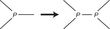
(37)

and hence can be regarded as an operator which inserts a vertex on an arbitrary connection in a network (See Fig.3). This is obviously the most fundamental operation which increases the number of vertices of a network.

Here we comment on our new proposal in comparison with the previous one [3]. Our main claim is that the multiplier should take ${\mathcal{N}}_{a}=\phi_{a}$ rather than “reasonable” choices such as ${\mathcal{N}}_{a}=P_{abb},\ P_{abc}P_{bed}P_{cde}$, etc., taken in the previous proposal. With ${\mathcal{N}}_{a}=\phi_{a}$, the Hamiltonian vector flow is uniquely determined by the dynamics, while “reasonable” choices are ambiguous. Even if ambiguous, there are no problems in the $N=2$ case, since there are no qualitative changes of the flow among “reasonable” choices, and the phase structure can uniquely be determined from the flow. However, as will be shown in Section 4, this is not true in general for $N>2$. In fact, $N=2$ is special for the following reasons. It is true that $\bar{\phi}_{a}$ can well be approximated by $\sim const.P_{abb}$ near the absorbing fixed points in Fig.2, because all of them can be shown to be gauge-equivalent to $P_{111}=1,\hbox{ others}=0$. This means that at least an approximate phase structure can be obtained even by putting ${\mathcal{N}}_{a}=P_{abb}\sim\bar{\phi}_{a}$. In addition, what makes the $N=2$ case very special is that the phase transition lines are the fixed points of the $Z_{2}$ symmetry corresponding to reversing the sign of the magnetic field of the Ising model on random networks. Therefore, the phase transition lines are protected by the symmetry, which stabilizes the qualitative properties of the flow under any changes of ${\mathcal{N}}_{a}$ respecting the symmetry.

Finally, we comment on an equation which can be derived from (24) in the thermodynamic limit. By putting $Z_{n}(P)\sim e^{-nf(P)}$ to (24), one can derive

$\displaystyle\bar{\phi}_{a}P_{abc}P_{bde}D^{P}_{cde}f(P)=-\frac{2}{3}e^{-f(P)+\frac{3}{2}}.$

(38)

In fact, one can directly prove (38). By using (9) and (10), the left-hand side of (38) is given by

	$\displaystyle\bar{\phi}_{a}P_{abc}P_{bde}D^{P}_{cde}f(P)$	$\displaystyle=\bar{\phi}_{a}P_{abc}P_{bde}(D^{P}_{cde}\bar{\phi}_{g})\frac{\partial f(P,\bar{\phi})}{\partial\bar{\phi}_{g}}-\bar{\phi}_{a}P_{abc}P_{bde}\frac{\bar{\phi}_{c}\bar{\phi}_{d}\bar{\phi}_{e}}{P\bar{\phi}^{3}}$
		$\displaystyle=-\frac{2}{3}P\bar{\phi}^{3},$		(39)

where we have used (11). This coincides with the right-hand side of (38), because of the choice (26) and $\bar{\phi}^{2}=\frac{3}{2}$, which can be obtained by contracting (11) with $\bar{\phi}_{a}$.

In this section, we will check the proposal of this paper in the cases of $N=2,3$ by comparing with the phase structures of the random tensor networks.

Let us first consider the $N=2$ case with a gauge,

$\displaystyle P_{111}=1,\ P_{112}=0.3,\ P_{122}=x_{1},\ P_{222}=x_{2},$

(40)

as a typical example. The difference from (7) is the gauge fixing value of $P_{112}$. One can obtain the phase structure in the parameter space of $(x_{1},x_{2})$ by studying the free energy (9). Alternatively, one can apply the $O(2)$ and scale transformations, (5) and (6), on $P$ so that the phase structure in the gauge (7) given in Fig.2 is transformed to that in the gauge (40). In either way, one can determine the phase structure in the new gauge, and the result is given in Fig.4. Here we draw the Hamilton vector flows for ${\mathcal{N}}_{a}=P_{abb}$, based on the former proposal, and ${\mathcal{N}}_{a}=\bar{\phi}_{a}$, based on our new proposal, in the left and right figures, respectively.

The rough features of the two flows based on the different proposals seem consistent with the phase structure: the flows depart from the transition lines, and go into the same absorption fixed points. This was the main argument in our previous paper [3]. However, there are some physically important differences in details between the left and the right figures. In the left figure, on the phase transition lines, the flow is going along them. Moreover, there exist a few fixed points of the flow on the transition lines at $(x_{1},x_{2})\sim(-0.2,1),(-0.6,0.5),(-0.4,-1)$ in the left figure. If the flow is strictly interpreted as a renormalization-group flow, the phase transition line on the righthand side of the fixed point near $(-0.2,1)$ is expected to be of second order, rather than first order, since the points on the both sides of the transition line in its vicinity flow to the same fixed point near $(0.1,0)$ without any discontinuities. On the other hand, in the right figure, the flow has discontinuity on the transition lines, except for the Curie point at the endpoint of the transition line. Thus, the flow based on our former proposal clearly contradicts the actual order of the phase transitions, while the one based our new proposal is in agreement with it, i.e. first order except for the Curie point.

An interesting property of the flow is that it does not vanish even on the Curie point, as can be seen in the right figure of Fig.4 and can also be checked numerically. This seems curious, because the second derivatives of the free energy contain divergences on the point. In a statistical system on a regular lattice, such divergences originate from an infinite correlation length. Therefore, such a point will typically become a fixed point of a renormalization-group flow. On the other hand, the correlation length of the Ising model on random networks is known to be finite even on the Curie point [28]. This means that, even starting from the Curie point, a renormalization process will bring the system to one with a vanishing correlation length. This implies that the Curie point cannot be a fixed point of a renormalization-group flow, and this is correctly reflected in the fact that our flow does not vanish on the Curie point.

Let us next consider the $N=3$ case. There seem to exist too many parameters to treat this case in full generality. So let us specifically consider a subspace parametrized by

$\displaystyle P_{iii}=1,\ P_{ijj}=x_{1},\ P_{123}=x_{2},\ \ (i\neq j),$

(41)

which is invariant under the $S_{3}$ transformation permuting the index labels, 1,2,3. Through numerical study of the free energy (9) (and some analytic considerations), one can obtain the phase structure shown in Fig.5. In the indicated parameter region, there exist two regions of an $S_{3}$ symmetric phase labeled by S with $\bar{\phi}_{1}=\bar{\phi}_{2}=\bar{\phi}_{3}$. There also exist two distinct non-symmetric phases labeled by NS1 and NS2. At any point in the two regions, the minimization of the free energy (10) has three distinct solutions of non-symmetric values, $\bar{\phi}_{1}\neq\bar{\phi}_{2}=\bar{\phi}_{3}$, $\bar{\phi}_{2}\neq\bar{\phi}_{3}=\bar{\phi}_{1}$, $\bar{\phi}_{3}\neq\bar{\phi}_{1}=\bar{\phi}_{2}$, and hence three distinct phases coexist in these regions. When $S_{3}$ symmetric subspace (41) is extended to more general cases, each of NS1 and NS2 becomes the common phase boundary of the three phases.

The flow in the left figure of Fig.5 is drawn based on our previous proposal ${\mathcal{N}}_{a}=P_{abb}$. There, the flow is not in good agreement with the phase structure, though it seems to capture some rough features. We tried other possibilities such as ${\mathcal{N}}_{a}=P_{abc}P_{bde}P_{cde}$, etc., but the flow depended on the choices, and no good agreement could be found. On the other hand, in the right figure based on our new proposal ${\mathcal{N}}_{a}=\bar{\phi}_{a}$, the flow in the symmetric region S is consistent with the phase structure: the flow departs from the transition lines, and, since it does not vanish on the lines, the order is expected to be first order. This is in agreement with the property of the free energy except for a point $(x_{1},x_{2})=(1/4,-1/8)$. At this point, the free energy is continuous in the first derivatives, but singular in the second. However, since the flow does not vanish on the point, the correlation length is expected to be finite. This is similar to the Curie point of the $N=2$ case.

In the non-symmetric phases, NS1 and NS2, the expectation values are not $S_{3}$ symmetric. Therefore, the flow has generally directions away from the $S_{3}$ symmetric subspace, and cannot be drawn on the figure. To also check the consistency of the flow in these regions, it would be necessary to extend the parameter region. This would require to take a different systematic strategy for consistency check to avoid too many parameters. In Section 6, we will take another way of consistency check by proving a theorem relating the renormalization group flow and the phase transitions of the random tensor network.

In Section 3, we argued that ${\cal O}=\phi_{a}{\mathcal{H}}_{a}$ provides a renormalization procedure for the random tensor network. As can be seen from (29) and (34), $P(s)$ diverges in the limit $s\rightarrow s_{\infty}$ in (30). On the other hand, in the numerical analysis of Section 4, $P$ is kept normalized as (40) and (41) by appropriately tuning the multiplier ${\mathcal{N}}$ for the scale transformation ${\mathcal{D}}$ (with ${\mathcal{N}}_{ab}{\mathcal{J}}_{ab}$ as well). As in Fig.4 and 5, one can find fixed points of the flows in the limit $\tilde{s}\rightarrow\infty$, where $\tilde{s}$ denotes the fictitious parameter parameterizing the normalized flows. In this section, we will show that these two limits of $s$ and $\tilde{s}$ are physically equivalent.

Let us first show the divergence in $s\rightarrow s_{\infty}$ more directly. Since $\bar{\phi}^{2}=\frac{3}{2}$ from (11), $\log P\bar{\phi}^{3}=-f(P)+\frac{3}{2}$. Then, by using (31) and (39), one obtains

$\displaystyle\frac{d}{ds}\log P\bar{\phi}^{3}=\frac{1}{3}P\bar{\phi}^{3},$

(42)

where $P$ is meant to be $P(s)$, and hence $P\bar{\phi}^{3}$ is regarded as a function of $s$. The solution to (42) is

$\displaystyle P\bar{\phi}^{3}=\frac{1}{\frac{1}{\left.P\bar{\phi}^{3}\right|_{s=0}}-\frac{s}{3}},$

(43)

which indeed diverges at $s=\frac{3}{\left.P\bar{\phi}^{3}\right|_{s=0}}=s_{\infty}$. Since $\bar{\phi}$ is normalized by $\bar{\phi}^{2}=\frac{3}{2}$, the divergence of (43) can be translated to the divergence of $P(s)$ with a behavior,

$\displaystyle P(s)\sim\frac{const.}{s_{\infty}-s},$

(44)

or higher order in the case that some components of $\bar{\phi}$ vanish in $s\rightarrow s_{\infty}$.

Now let us compare the two flows, unnormalized and normalized ones. For notational simplicity, let us denote the three indices of $P_{abc}$ by one index as $P_{i}$. The flow equations in $s$ and $\tilde{s}$ can respectively be expressed as

		$\displaystyle\frac{d}{ds}P_{i}(s)=\bar{\phi}_{a}(P(s))\,g_{ai}(P(s)),$		(45)
		$\displaystyle\frac{d}{d\tilde{s}}\tilde{P}_{i}(\tilde{s})=\bar{\phi}_{a}(\tilde{P}(\tilde{s}))\,g_{ai}(\tilde{P}(\tilde{s}))-{\mathcal{N}}\tilde{P}_{i}(\tilde{s}),$		(46)
		$\displaystyle P_{i}(s=0)=\tilde{P}_{i}(\tilde{s}=0)=P_{i},$		(47)

where ${\mathcal{N}}$ generally depends on $\tilde{P}_{i}(\tilde{s})$, and $g_{ai}(P)$ are the quadratic polynomial functions of $P$, which can be read from (35). The last term of the second equation comes from ${\mathcal{N}}{\mathcal{D}}$ in (20), and is assumed to be tuned to satisfy a gauge condition normalizing $\tilde{P}(\tilde{s})$. Here we ignore the $SO(N)$ generators, ${\mathcal{J}}_{ab}$, for simplicity, but it is not difficult to extend the following proof to include them.

The physical properties of the random tensor network do not depend on the overall scale of $P$. So let us define the relative values of $P(s)$ and $\tilde{P}(\tilde{s})$ as

$\displaystyle Q_{i}(s)=\frac{P_{i}(s)}{P_{0}(s)},\ \ \ \tilde{Q}_{i}(\tilde{s})=\frac{\tilde{P}_{i}(\tilde{s})}{\tilde{P}_{0}(\tilde{s})},$

(48)

where $P_{0}(s)\ (\tilde{P}_{0}(\tilde{s}))$ is taken from one of $P_{i}(s)\ (\hbox{resp.}\tilde{P}_{i}(\tilde{s}))$, or a linear combination of them. From (11), it is obvious that $\bar{\phi}(P)$ and $\bar{\phi}(\tilde{P})$ actually depend only on $Q$ and $\tilde{Q}$, respectively. Then, from (45),

	$\displaystyle\frac{1}{P_{0}}\frac{d}{ds}Q_{i}$	$\displaystyle=\frac{1}{P_{0}}\frac{d}{ds}\frac{P_{i}}{P_{0}}$
		$\displaystyle=\frac{\bar{\phi}_{a}(Q)\,g_{ai}(P)}{P_{0}^{2}}-\frac{\bar{\phi}_{a}(Q)\,g_{a0}(P)P_{i}}{P_{0}^{3}}$
		$\displaystyle=\bar{\phi}_{a}(Q)\left(g_{ai}(Q)-g_{a0}(Q)Q_{i}\right).$		(49)

In the same manner,

$\displaystyle\frac{1}{\tilde{P}_{0}}\frac{d}{ds}\tilde{Q}_{i}=\bar{\phi}_{a}(\tilde{Q})\left(g_{ai}(\tilde{Q})-g_{a0}(\tilde{Q})\tilde{Q}_{i}\right).$

(50)

Note that the last term of (46) does not contribute to the flow equation of $\tilde{Q}$. Since the initial condition (47) implies $Q_{i}(s=0)=\tilde{Q}_{i}(\tilde{s}=0)$, and the righthand sides of (49) and (50) are identical, the flow equations, (49) and (50), describe an identical flow with a transformation between the fictitious parameters,

$\displaystyle P_{0}(s)ds=\tilde{P}_{0}(\tilde{s})d\tilde{s}.$

(51)

As discussed above, the typical behavior of $P_{0}(s)$ is (44), while $\tilde{P}_{0}(\tilde{s})$ is assumed to remain finite near an absorption fixed point. In such a case, (51) implies

$\displaystyle\tilde{s}\sim-const.\log(s_{\infty}-s).$

(52)

Therefore, the limits of $s\rightarrow s_{\infty}$ and $\tilde{s}\rightarrow\infty$ are physically equivalent. As can be checked easily, this physical implication does not change, even if we consider the case that $P_{0}(s)$ diverges with an order higher than (44).

To investigate the physical meaning of the fictitious parameter $\tilde{s}$, let us estimate (29) near $s\sim s_{\infty}$. We obtain

	$\displaystyle\sum_{m=0}^{\infty}\frac{s^{m}(n+m-1)!}{3^{m}m!(n-1)!}e^{-(n+m)f(P)+\frac{3m}{2}}$	$\displaystyle=\frac{e^{-nf(P)}}{(n-1)!}\sum_{m=0}^{\infty}(m+1)(m+2)\cdots(n+m-1)\left(\frac{s}{s_{\infty}}\right)^{m}$
		$\displaystyle=const.\frac{d^{n-1}}{ds^{n-1}}\sum_{m=0}^{\infty}\left(\frac{s}{s_{\infty}}\right)^{m+n-1}$
		$\displaystyle=const.\frac{d^{n-1}}{ds^{n-1}}\frac{s^{n-1}}{s_{\infty}-s}$
		$\displaystyle\sim const.(s_{\infty}-s)^{-n}$		(53)

Then the average size of networks can be estimated as

$\displaystyle\langle n+m\rangle\sim n+s\frac{d}{ds}\log(s_{\infty}-s)^{-n}\sim\frac{ns_{\infty}}{s_{\infty}-s}.$

(54)

Therefore

$\displaystyle\tilde{s}\sim const.\log\left(\hbox{Average size}\right).$

(55)

This means that $\tilde{s}$ corresponds to the standard renormalization-group scale parameter often denoted by $\log\Lambda$ in field theory.

In Section 4, we see that the renormalization-group flow has discontinuity on the first-order phase transition lines in the examples of the random tensor networks. In this section, we will prove a general theorem on this aspect.

By using the free energy in the thermodynamic limit (9), the stationary condition (11) and the flow equation (35), we can prove the following theorem.

Theorem: The following three statements are equivalent.

• (i)

  The first derivatives of $f(P)$ are continuous at $P$.

• (ii)

  $\bar{\phi}$ is continuous at $P$.

• (iii)

  The renormalization-group flow is continuous at $P$.

Proof: Let us first prove $\hbox{(i)}\Rightarrow\hbox{(ii)}$. From (9), the first derivatives of $f(P)$ are given by

$\displaystyle D^{P}_{abc}f(P)=-\frac{\bar{\phi}_{a}\bar{\phi}_{b}\bar{\phi}_{c}}{P\bar{\phi}^{3}},$

(56)

where we have neglected the contributions from the $P$-dependence of $\bar{\phi}$, since $\bar{\phi}$ satisfies the stationary condition (11). By contracting a pair of indices in (56), one obtains,

$\displaystyle D^{P}_{aab}f(P)=-\frac{\bar{\phi}_{a}\bar{\phi}_{a}\bar{\phi}_{b}}{P\bar{\phi}^{3}}=-\frac{3\bar{\phi}_{b}}{2P\bar{\phi}^{3}},$

(57)

where we have used $\bar{\phi}^{2}=\frac{3}{2}$ derived from (11). Here note that $P\bar{\phi}^{3}$ is continuous at any $P$, because the free energy $f(P)$ itself in (9) is continuous at any $P$^**** ** This can be proven by using that $f(P)$ is the minimum of (10), which is a continuous function of $\phi$ and $P$., and also $\bar{\phi}^{2}=\frac{3}{2}$. Therefore, if (i) holds, (57) is continuous and hence $\bar{\phi}$ is continuous; $\hbox{(i)}\Rightarrow\hbox{(ii)}$ has been proven.

References

- [1] K. G. Wilson, “The Renormalization Group: Critical Phenomena and the Kondo Problem,” Rev. Mod. Phys. 47 (1975) 773.
- [2] K. G. Wilson and J. B. Kogut, “The Renormalization group and the epsilon expansion,” Phys. Rept. 12 (1974) 75.
- [3] N. Sasakura and Y. Sato, “Ising model on random networks and the canonical tensor model,” PTEP 2014, no. 5, 053B03 (2014) [arXiv:1401.7806 [hep-th]].
- [4] N. Sasakura and Y. Sato, “Exact Free Energies of Statistical Systems on Random Networks,” SIGMA 10, 087 (2014) [arXiv:1402.0740 [hep-th]].
- [5] N. Sasakura, “Canonical tensor models with local time,” Int. J. Mod. Phys. A 27 (2012) 1250020 [arXiv:1111.2790 [hep-th]].
- [6] N. Sasakura, “Uniqueness of canonical tensor model with local time,” Int. J. Mod. Phys. A 27 (2012) 1250096 [arXiv:1203.0421 [hep-th]].
- [7] N. Sasakura, “A canonical rank-three tensor model with a scaling constraint,” Int. J. Mod. Phys. A 28 (2013) 1 [arXiv:1302.1656 [hep-th]].
- [8] J. Ambjorn, B. Durhuus and T. Jonsson, “Three-Dimensional Simplicial Quantum Gravity And Generalized Matrix Models,” Mod. Phys. Lett. A 6, 1133 (1991).
- [9] N. Sasakura, “Tensor Model For Gravity And Orientability Of Manifold,” Mod. Phys. Lett. A 6, 2613 (1991).
- [10] N. Godfrey and M. Gross, “Simplicial Quantum Gravity In More Than Two-Dimensions,” Phys. Rev. D 43, 1749 (1991).
- [11] R. Gurau, “Colored Group Field Theory,” Commun. Math. Phys. 304 (2011) 69 [arXiv:0907.2582 [hep-th]].
- [12] R. Gurau and J. P. Ryan, “Colored Tensor Models - a review,” SIGMA 8, 020 (2012) [arXiv:1109.4812 [hep-th]].
- [13] R. Gurau, “The 1/N Expansion of Tensor Models Beyond Perturbation Theory,” Commun. Math. Phys. 330, 973 (2014) [arXiv:1304.2666 [math-ph]].
- [14] V. Rivasseau, “The Tensor Track, III,” Fortsch. Phys. 62, 81 (2014) [arXiv:1311.1461 [hep-th]].
- [15] J. Ben Geloun, “Renormalizable Models in Rank Tensorial Group Field Theory,” Commun. Math. Phys. 332, 117 (2014) [arXiv:1306.1201 [hep-th]].
- [16] D. Oriti, “Group Field Theory and Loop Quantum Gravity,” arXiv:1408.7112 [gr-qc].
- [17] D. Ousmane Samary, “Beta functions of gauge invariant just renormalizable tensor models,” Phys. Rev. D 88, no. 10, 105003 (2013) [arXiv:1303.7256 [hep-th]].
- [18] A. Eichhorn and T. Koslowski, “Continuum limit in matrix models for quantum gravity from the Functional Renormalization Group,” Phys. Rev. D 88, 084016 (2013) [arXiv:1309.1690 [gr-qc]].
- [19] M. Raasakka and A. Tanasa, “Next-to-leading order in the large expansion of the multi-orientable random tensor model,” arXiv:1310.3132 [hep-th].
- [20] S. Carrozza, “Discrete Renormalization Group for SU(2) Tensorial Group Field Theory,” arXiv:1407.4615 [hep-th].
- [21] J. Ben Geloun and R. Toriumi, “Parametric Representation of Rank d Tensorial Group Field Theory: Abelian Models with Kinetic Term ,” arXiv:1409.0398 [hep-th].
- [22] V. A. Nguyen, S. Dartois and B. Eynard, “An analysis of the intermediate field theory of tensor model,” arXiv:1409.5751 [math-ph].
- [23] D. Benedetti, J. Ben Geloun and D. Oriti, “Functional Renormalisation Group Approach for Tensorial Group Field Theory: a Rank-3 Model,” arXiv:1411.3180 [hep-th].
- [24] T. Delepouve and V. Rivasseau, “Constructive Tensor Field Theory: The Model,” arXiv:1412.5091 [math-ph].
- [25] N. Sasakura and Y. Sato, “Interpreting canonical tensor model in minisuperspace,” Phys. Lett. B 732, 32 (2014) [arXiv:1401.2062 [hep-th]].
- [26] N. Sasakura, “Quantum canonical tensor model and an exact wave function,” Int. J. Mod. Phys. A 28 (2013) 1350111 [arXiv:1305.6389 [hep-th]].
- [27] G. Narain, N. Sasakura and Y. Sato, “Physical states in the canonical tensor model from the perspective of random tensor networks,” JHEP 1501, 010 (2015) [arXiv:1410.2683 [hep-th]].
- [28] See, S. N. Dorogovtsev, A. V. Goltsev, J. F. F. Mendes, “Critical phenomena in complex networks,” Rev. Mod. Phys. 80, 1275 (2008) [arXiv:0705.0010 [cond-mat]], and references therein for the dynamics of statistical systems on random networks.
- [29] R. L. Arnowitt, S. Deser and C. W. Misner, “Canonical variables for general relativity,” Phys. Rev. 117, 1595 (1960); R. L. Arnowitt, S. Deser and C. W. Misner, “The Dynamics of general relativity,” arXiv:gr-qc/0405109.
- [30] For instance, see N. Goldenfeld, “Lectures on Phase Transitions and the Renormalization Group,” ISBN-020155408955408.
- [31] For instance, see A. D. Sokal, A. C. D. van Enter and R. Fernandez, “Renormalization transformations in the vicinity of first-order phase transitions: What can and cannot go wrong,” Phys. Rev. Lett. 66, 3253 (1991), and references therein.