Error Correcting Index Codes and Matroids

The index coding problem introduced by Birk and Kol [1] involves a source which generates a set of messages and a set of receivers which demand messages. Each receiver has prior knowledge of a portion of the message called side-information, which is known to the source. The source uses the knowledge of the side-information available at all the receivers to find a transmission scheme of minimum number of transmissions, which satisfies all the demands of the receivers. Bar-Yossef et al. [2] studied the index coding problem and found that the length of the optimal linear index code is equal to the minrank of a related graph.

The connection between multi-linear representation of matroids and index coding was studied by El Rouayheb, Sprinston and Georghiades [3]. It was shown by Muralidharan and Rajan [4] that a vector linear solution to an index coding problem exists if and only if there exists a representable discrete polymatroid satisfying certain conditions which are determined by the index coding problem.

The problem of index coding with erroneous transmissions was studied by Dau et al. [5]. An index code capable of correcting at most $\delta$-errors at all its receivers is defined as a $\delta$-error correcting index code. The necessary and sufficient conditions for a scalar linear index code to have $\delta$-error correcting capability was found. Network linear network error-correcting codes were introduced earlier by Yeung and Cai [6],[7]. The link between network error correcting and matroid theory was established by Prasad and Rajan in [8].

Index coding problems are modeled in the following way. There is a unique source $S$ having message $\mathbf{\mathit{x}}=(\mathit{x_{1}},\mathit{x_{2}}\ldots,\mathit{x_{n}})\in\mathbb{F}_{q}^{n}$, where $\mathbb{F}_{q}$ is a finite field of $q$ elements. There are $m$ receivers $R_{1},R_{2},\ldots,R_{m}$. Let $\left\lceil n\right\rfloor$ denote the set $\left\{1,2,\ldots,n\right\}$. Each $R_{i}$ possesses a set of messages $\{x_{j}\}_{j\in\chi_{i}}$, where $\chi_{i}\subseteq\left\lceil n\right\rfloor$. Let $\chi=\{\chi_{1},\chi_{2},\ldots,\chi_{m}\}$ represents the set of side information possessed at all receivers. Each receiver $R_{i}$ demands a single message $x_{f(i)}$. The mapping $f:\left\lceil m\right\rfloor\rightarrow\left\lceil n\right\rfloor$ satisfies $f(i)\notin\chi_{i}$. So an index coding problem is described by the quadruple $(m,n,\chi,f)$. The objective is to find an encoding scheme referred to as an index code that satisfies all receivers and uses minimum number of transmissions.

Note that the encoding function $\mathfrak{C}:\mathbb{F}_{q}^{n}\rightarrow\mathbb{F}_{q}^{N}$, can be viewed as $N$ encoding functions $c_{1},c_{2},\ldots,c_{N}$, where each $c_{i}$ is a function from $\mathbb{F}_{q}^{n}\rightarrow\mathbb{F}_{q}$. For the source message $x\in\mathbb{F}_{q}^{n}$, $c_{i}(x)$ gives the $i^{th}$ transmission of the index code. So an $N$ length index code $\mathfrak{C}$ can also be described by set of $N$ functions $\{c_{1},c_{2},\ldots,c_{N}\}$, denoted by $S(\mathfrak{C})$.

Rouayheb et al. [3] proved that the index coding problem has a solution if and only if the equivalent network coding problem is solvable. The equivalent network coding problem for the index coding problem is as follows. Consider an instance of the index coding problem described by the quadruple $(m,n,\chi,f)$ with an index code $\mathfrak{C}$ of length $N$. The corresponding equivalent network coding problem for the index coding problem $(m,n,\chi,f)$ and index code $\mathfrak{C}$ is given in Fig. 1. The equivalent network coding problem has $n$ source nodes each corresponding to the source messages of the index coding problem. There are two levels of intermediate nodes denoted by $w_{i}$ and $w^{\prime}_{i}$ for $i=1$ to $N$. Each node $w_{i}$ has $n$ incoming edges, one from each of the source nodes. Each node $w^{\prime}_{i}$ has only one input edge $e_{i}$, from $w_{i}$. The nodes $R_{1},R_{2},\ldots,R_{m}$ are the receiver nodes. Each receiver node $R_{i}$ has two types of input edges, $N$ input edges from each of the $w^{\prime}_{i}$ node and there are $|\chi_{i}|$ input edges which correspond to the side information possessed by the receiver. The edges corresponding to side information are represented as dashed lines in the figure. The side information edges for a receiver $R_{i}$ are the edges $(x_{j},R_{i})$ for $j\in\chi_{i}$. The information flowing through the edge $e_{i}$ of the equivalent network corresponds to the $i^{th}$ transmission of the index code $\mathfrak{C}$. The problem of index coding with error correction with receivers capable of correcting at most $\delta$ errors can be transformed to a network error correcting problem. Hence, a natural question that arise is whether it is possible to link index codes and representable matroids by first transforming the index coding problem into equivalent network coding problem as in [3] and then link error correcting network code to matroids as in [8]. If one takes this approach then, in the equivalent network, network code should be able to correct $m\delta$ errors as each receiver has $\delta$ error correcting capability. Also these errors are restricted to certain edges of the equivalent network. The errors can occur only in the edges between $w^{\prime}_{i}$ and receiver nodes. Among the $N$ edges between $w^{\prime}_{i}$ and $R_{j}$, at most $\delta$ can be in error. There are $m$ receivers and hence at most $m\delta$ errors. Such case of restriction of errors to a subset of edges was not considered earlier. We also note that the size of the ground set of the matroid for which we have to find representation is smaller compared to the matroid obtained from the equivalent network coding problem. If we consider $m\delta$ errors without any restriction and equivalent network the size of the ground set of the matroid obtained is $n+2|\mathcal{E}|$, where $\mathcal{E}$ is the edge set of the equivalent network. Number of edges in the equivalent network for an index coding problem $(m,n,\chi,f)$ is $|\mathcal{E}|=(n+m+1)N+\overset{m}{\underset{i=1}{\sum}}|\chi_{i}|$. The matroid which we obtain has a ground set of cardinality only $n+2N$ which is much smaller than $n+2|\mathcal{E}|$.

The contributions of this paper are as follows.

• •

  We define differential error correcting index code in which the receivers have different error correcting capability. The necessary and sufficient conditions for a matrix $L$ to correspond to a differential index code is found.

• •

  We establish a link between linear differential error correcting index codes and certain matroids. We define a matroidal differential error correcting index code and show that a linear differential error correcting index code exists if and only if it is matroidal differential error correcting index code associated with a representable matroid.

• •

  We consider two special cases, $\delta$-error correcting index codes and error correction at a subset of receiver nodes. The representable matroids associated with these two special cases are identified.

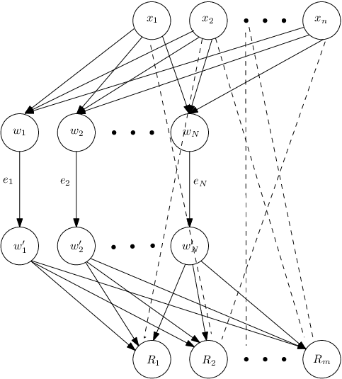
The organization of the paper is as follows. In Section II we review the definitions of error correcting index codes. We define differential error correcting index codes and also establishes a lemma which is used to prove our main result. In Section III, basic results of Matroids are reviewed. Finally in Section IV, we define matroidal differential error correcting index code and establishes the link between matroids and differential error correcting index codes. We conclude and summarize all the results in Section V.

Notations: The size of a set $S$ is denoted by $|S|$. Consider two sets $S_{1}$ and $S_{2}$. The set subtraction $S_{1}\setminus S_{2}$ is denoted by $S_{1}-S_{2}$. The rank of a matrix $A$ over $\mathbb{F}_{q}$ is denoted by $rank(A)$. For some positive integer $N$, identity matrix of size $N$ over $\mathbb{F}_{q}$ is denoted by $I_{N}$. The vector space spanned by columns of a matrix $A$ over $\mathbb{F}_{q}$ is denoted by $\langle A\rangle$. Consider a vector $x=(x_{1},x_{2},\ldots,x_{n})\in\mathbb{F}_{q}^{n}$. The support of vector $x$ is defined to be the set $supp(x)=\{i\in\lceil n\rfloor:x_{i}\neq 0\}.$ The Hamming weight of a vector $x$, denoted by $wt(x)$, is defined to be the $|supp(x)|$. For some subset $B=\{i_{1},i_{2},\ldots,i_{b}\}$ of $\lceil n\rfloor$, where $i_{1}<i_{2}<\ldots<i_{b}$, let $x_{B}$ denote the vector $(x_{i_{1}},x_{i_{2}},\ldots,x_{i_{b}})$. For some matrix $A$, $A^{(i)}$ denotes the $i^{th}$ column of $A$. For a set of column indices $\mathcal{I}$, $A^{\mathcal{I}}$ denotes the submatrix of $A$ with columns indexed by $\mathcal{I}$. Similarly $A_{(j)}$ denotes the $j^{th}$ row of $A$ and for a set of row indices $\mathcal{J}$, $A_{\mathcal{J}}$ denotes the submatrix of $A$ with rows indexed by $\mathcal{J}$.

In this section, we review error correcting index codes, define differential error correcting index code and establish a lemma which we use in Section IV to establish our main result.

Error correcting index codes consider the scenario in which the symbols received by receiver $R_{i}$ may be subject to errors. The source $S$ broadcasts a vector $\mathfrak{C}(x)\in\mathbb{F}_{q}^{N}$. The error affecting receiver $R_{i}$ is considered as an additive error represented by $\epsilon_{i}\in\mathbb{F}_{q}^{N}$. Then, $R_{i}$ actually receives the vector $y_{i}=\mathfrak{C}(x)+\epsilon_{i}\in\mathbb{F}_{q}^{N}$. An error correcting index code should be able to satisfy the demands of receivers in the presence of these additive errors.

If the encoding function $\mathfrak{C}$ is linear then it is a linear error correcting index code. As for the linear index code, linear error correcting index code can also be described by a matrix $L$.

Dau et al. in [5] identify a necessary and sufficient condition which a matrix $L$ has to satisfy to correspond to a $\delta$-error correcting index code. Consider the set of vectors

Here $\mathcal{H}$ is a directed hypergraph [9] used to describe the index coding problem $(m,n,\chi,f)$. The necessary and sufficient conditions for a matrix $L$ to correspond to a $\delta$-error correcting index code is as follows. The matrix $L$ corresponds to a $(\delta,\mathcal{H})$-ECIC over $\mathbb{F}_{q}$ if and only if

The proof of (1) follows from the fact that if (1) is not satisfied then one can demonstrate the existence of a pair of information vectors $x$ and $x^{\prime}$ with $x_{f(i)}\neq x^{\prime}_{f(i)},x_{\chi_{i}}=x^{\prime}_{\chi_{i}}$ and a corresponding pair of error vectors $\epsilon$ and $\epsilon^{\prime}$ with $wt(\epsilon)\leq\delta$ and $wt(\epsilon^{\prime})\leq\delta$ such that the corresponding received vectors at receiver $R_{i}$ are equal. So the receiver $R_{i}$ will not be able to distinguish between $x_{f(i)}$ and $x^{\prime}_{f(i)}$. Therefore, $L$ corresponds to a $\delta$-error correcting index code if and only if the following condition holds. For all $i\in\lceil m\rfloor$ and for all $z\in\mathbb{F}_{q}^{n}$ such that $z_{\chi_{i}}=0$ and $z_{f(i)}\neq 0$, $zL+e\neq 0,\forall~e\in\mathbb{F}_{q}^{N},wt(e)\leq 2\delta$. This equation can be rewritten in matrix form in the following way. For each receiver $R_{i}$

The matrix $L$ corresponds to an error correcting index code if and only if (2) is satisfied at all receivers $R_{i},$ $i\in\lceil m\rfloor$.

We now define a differential $\delta_{R}$ error correcting index code. A differential error correcting index coding problem considers the scenario in which the error correcting capability varies from receiver to receiver.

Equation (2) needs to be modified for the differential $\delta_{R}$ error correcting index code. A matrix $L$ corresponds to a differential error correcting index code if and only if the following condition holds. For each receiver $R_{i},i\in\lceil m\rfloor$,

The error pattern corresponding to an error vector $e$ is defined as its support set $supp(e)$. Let $\mathbb{I}_{supp(e)}$ denote the submatrix of $I_{N}$ consisting of those rows of $I_{N}$ indexed by $supp(e)$. For a receiver $R_{i}$, the error correcting condition (3) can be rewritten as

Let $\overline{\chi_{i}}$ denote the set $\lceil n\rfloor-\chi_{i}$. Since at a particular receiver we consider only those $z\in\mathbb{F}_{q}^{n}$ for which $z_{\chi_{i}}=0$ condition (4) can be rewritten as

We now present a lemma which will be used in Section IV to prove the main result of this paper.

Lemma 1 gives an equivalent condition for equation (4). Therefore a given index code is differential $\delta_{R}$ error correcting if and only if (7) holds for all $supp(e)\in\{\mathcal{F}\subseteq\lceil N\rfloor:|\mathcal{F}|=2\delta_{i}\}$ and at all receivers $R_{i},i\in\lceil m\rfloor$.

In this section we list few basic definitions and results from matroid theory. These results and definitions are taken from [10].

The set $E$ is called the ground set of the matroid and is also referred to as $E(\mathcal{M})$. The members of set $\mathcal{I}$ are called the independent sets of $\mathcal{M}$. Independent sets are also denoted by $\mathcal{I}(\mathcal{M})$. A maximal independent subset of $E$ is called a basis of $\mathcal{M}$ and the set of all bases of $\mathcal{M}$ is denoted by $\mathcal{B}(\mathcal{M})$. With $\mathcal{M}$, a function called the rank function is associated, whose domain is the power set of $E$ and codomain is the set of non-negative integers. The rank of any $X\subseteq E$ in $\mathcal{M}$, denoted by $r_{\mathcal{M}}(X)$ is defined as the maximum cardinality of a subset $X$ that is a member of $\mathcal{I}(\mathcal{M})$. The rank of matroid is the rank of its ground set.

Consider a matroid $\mathcal{M}$ with matrix $A$ as its representation. Each element in ground set of $\mathcal{M}$ corresponds to a column in $A$. For a subset $S$ of ground set $E(\mathcal{M})$, $A^{S}$ denotes the submatrix of $A$ with columns corresponding to the elements of ground set in $S$.

The contraction of a $\mathbb{F}$-representable matroid is also $\mathbb{F}$-representable. Let $\mathcal{M}[A]$ be the vector matroid associated with a matrix $A$ over $\mathbb{F}$. Let $e$ be the index of a non-zero column of $A$. Suppose using the elementary row operations, we transform $A$ to obtain a matrix $A^{\prime}$ which has a single non-zero entry in column $e$. Let $A^{\prime\prime}$ denote the matrix which is obtained by deleting the row and column containing the only non-zero entry of column $e$. Then $\mathcal{M}[A]/\{e\}=\mathcal{M}[A^{\prime\prime}].$

In this section we first define matroidal differential error correcting index codes and then prove the main result of the paper.

Definition 8 can be viewed as a matroidal abstraction of differential $\delta_{R}$ error correcting index codes. Condition (A) ensures that the vectors representing the messages are linearly independent. Condition (B) is equivalent to the condition that scalar linear index code should be a non-zero linear combination of messages added with a linear combination of errors. Condition (C) ensures that the receivers can decode their demands in the presence of errors. Condition (C) requires that $g(\{c_{1},c_{2},\ldots,c_{N}\})$ and $g(f(i))$ is present in $E(\mathcal{M}_{\mathcal{F},i})$. However this is ensured because condition (B) ensures $g(\{c_{1},c_{2},\ldots,c_{N}\})$ does not belong to $B$ and hence it is not contracted out. Also since $g(f(i))\subseteq g(\overline{\chi_{i}})$, it is also not contracted out of the matroid $\mathcal{M}$. We now present the main result of this paper which relates scalar linear differential error correcting index codes to representable matroids.

Theorem 1 establishes a link between scalar linear differential $\delta_{R}$ error correcting index codes and a representable matroid satisfying certain properties. In the examples below, we consider differential error correcting index coding problems with a scalar linear solution and show the representable matroid associated with it.

In this paper we have defined differential error correcting index codes which is a generalization of error correcting index codes. We established the connections between differential error correcting index codes and matroids. It was shown that scalar linear differential error correcting codes correspond to representable matroid with certain properties. This sheds lots of light in construction and existence of differential error correcting codes for an index coding problem. The definition of a matroidal differential error correcting index code is more general and the matroid need not be a representable matroid. Using a non representable matroid satisfying the conditions, the possibility of non linear differential error correcting codes could be explored.

References

- [1] Y. Birk and T. Kol,“Informed-source coding-on-demand (ISCOD) over broadcast channels,”in Proc. IEEE Conf. Comput. Commun., San Francisco, CA, 1998, pp.1257-1264.
- [2] Z. Bar-Yossef, Z. Birk, T. S. Jayram and T. Kol, “Index coding with side information,” in Proc. 47th Annu. IEEE Symp. Found. Comput. Sci., 2006, pp. 197-206.
- [3] S. E. Raouayheb, A. Sprinston and C. Georghiades, “On the Index coding problem and its relation to network coding and matroid theory,” in IEEE Trans. Inf. Theory, vol 56, no. 7, pp . 3187-3195, July 2010.
- [4] V. T. Muralidharan and B. S. Rajan, “Linear Network Coding, Linear index coding and representable discrete polymatroids,”, Available on ArXiv at http://arxiv.org/abs/1306.1157.
- [5] Son Hoang Dau, Vitaly Skachek and Yeow Meng Chee, “Error Correction for Index Coding with Side Information,” in IEEE Transactions on Information Theory, Vol. 59, No. 3,March 2013.
- [6] R. W. Yeung and N. Cai, “Network error correction, part I: basic concepts and upper bounds,” in Comm. in Inform. and Systems, vol. 6, 2006, pp. 19-36.
- [7] R. W. Yeung and N. Cai, “Network error correction, part II: lower bounds,” in Comm. in Inform. and Systems, vol. 6, 2006, pp. 37-54.
- [8] K. Prasad and B. S. Rajan, “A Matroidal framework for Network-Error Correcting Codes,” IEEE Transactions on Information Theory, Vol.61, No. 2, pp. 836-872, February 2015.
- [9] N. Alon, A. hassidimi, E. Lubetzky,U. Stav and A. Weinsten, “Broadcasting with side information,” in Proc. 49th Annu. IEEE Symp. Found. Comput. Sci., 2008, pp. 823-832.
- [10] J. G. Oxley, “Matroid Theory”, Oxford University Press, 1992.
Appendix A Proof of Lemma 1
Lemma 1 : Let denote length vector with a in one of the first position corresponding to the demand of the receiver , and with all other elements . For some the condition