Edge reconstruction in armchair phosphorene nanoribbons revealed by discontinuous Galerkin density functional theory
Wei Hu,∗a Lin Lin,∗ba and Chao Yang∗a
Received Xth XXXXXXXXXX 20XX,
Accepted Xth XXXXXXXXX 20XX
First published on the web Xth
XXXXXXXXXX 200X
DOI: 00.0000/00000000
With the help of our recently developed massively parallel DGDFT (Discontinuous Galerkin Density Functional Theory) methodology, we perform large-scale Kohn-Sham density functional theory calculations on phosphorene nanoribbons with armchair edges (ACPNRs) containing a few thousands to ten thousand atoms. The use of DGDFT allows us to systematically achieve conventional plane wave basis set type of accuracy, but with a much smaller number (about 15) of adaptive local basis (ALB) functions per atom for this system. The relatively small number degrees of freedom required to represent the Kohn-Sham Hamiltonian, together with the use of the pole expansion the selected inversion (PEXSI) technique that circumvents the need to diagonalize the Hamiltonian, result in a highly efficient and scalable computational scheme for analyzing the electronic structures of ACPNRs as well as its dynamics. The total wall clock time for calculating the electronic structures of large-scale ACPNRs containing 1080-10800 atoms is only 10-25 s per self-consistent field (SCF) iteration, with accuracy fully comparable to that obtained from conventional planewave DFT calculations. For the ACPNR system, we observe that the DGDFT methodology can scale to 5,000-50,000 processors. We use DGDFT based ab-initio molecular dynamics (AIMD) calculations to study the thermodynamic stability of ACPNRs. Our calculations reveal that a 2 1 edge reconstruction appears in ACPNRs at room temperature.
1 Introduction
Kohn-Sham density functional theory (DFT)1, 2 is the most widely used methodology for performing ab initio electronic structure calculations to study the structural and electronic properties of molecules, solids and nanomaterials. However, until recently, DFT calculations are limited to small systems because they have a relatively high complexity () with the system size . As the system size increases, the cost of traditional DFT calculations becomes prohibitively expensive. Therefore, it is still challenging to use DFT calculations to treat large-scale systems that may contain thousand or tens of thousands of atoms. Although various linear scaling methods3, 4, 5 have been proposed for improving the efficiency of DFT calculations, they rely on the nearsightedness principle, which leads to exponentially localized density matrices in real-space for systems with a finite energy gap or at finite temperature. On the other hand, most of the existing linear scaling DFT codes, such as SIESTA,6 CONQUEST,7 OPENMX8 and HONPAS,9 are based on the contracted and localized basis sets in the real-space, such as Gaussian-type orbitals or numerical atomic orbitals.4It is relatively difficult to improve the accuracy of methods based on such contracted basis functions in a systematic fashion compared to methods based on conventional uniform basis sets, for example, the planewave basis set,10. The disadvantage of using uniform basis sets is the relatively large number of basis functions required per atom.
Recently, we have developed a massively parallel DGDFT (Discontinuous Galerkin Density Functional Theory) methodology for performing efficient large-scale Kohn-Sham DFT calculations. The methodology is based on the combination of the adaptive local basis (ALB) set11 and the pole expansion and selected inversion (PEXSI) technique.12, 13, 14 The ALB functions are localized in the real space and discontinuous in the global domain. The continuous Kohn-Sham orbitals and density are assembled from the discontinuous basis functions using the discontinuous Galerkin (DG) method.15, 16 Because it is rooted in a domain decomposition approach that takes the chemical environment effects into account, the ALB set constructed by the DGDFT methodology is systematically improvable. It can achieve the same level of accuracy obtained by conventional plane wave calculations with much fewer number of basis functions. The sparse Hamiltonian matrix generated from DGDFT can take advantage of the PEXSI method. The PEXSI method overcomes the scaling limit for solving Kohn-Sham DFT, and scales at most as even for metallic systems at room temperature. In particular, the computational complexity of the PEXSI method is only for 1D systems, and is for 2D systems. This also makes the DGDFT methodology particularly suitable for analyzing low-dimensional (1D and 2D) systems regardless whether the system is a metal, a semiconductor or an insulator.13
In this paper, we demonstrate the accuracy and efficiency of DGDFT by using it to analyze the electronic structures and thermodynamic stability of armchair phosphorene nanoribbons (ACPNRs), which is an interesting 1D derivative of phosphorene with some remarkable properties. We use DGDFT to perform both static electronic structure calculations as well as ab initio molecular dynamics (AIMD) calculations. Our AIMD calculations reveal that a edge reconstruction appears in the edge unpassivated ACPNRs at room temperature.
The paper is organized as follows. In section 2, we introduce our recently developed massively parallel DGDFT methodology for efficient large-scale Kohn-Sham DFT based electronic structure calculations. In section 3, we provide some background on phosphorene nanoribbons that we examine. We report the results obtained from applying DGDFT to ACPNRs in section 4. We demonstrate that the DGDFT methodology can achieve high accuracy with much fewer basis functions compared to the conventional planewave discretized calculations. We also show that DGDFT can handle large ACPNRs systems with thousand or even tens of thousands of atoms. Furthermore, we show that the DGDFT methodology is highly scalable on modern high performance computers because it contains multiple levels of parallelization. Finally, we show that by using DGDFT based ab-initio molecular dynamics (AIMD) calculations, we are able to identify a 2 1 edge reconstruction in the edge-unpassivated ACPNRs at room temperature. This observation suggests that PNRs may modify their electronic structures over time, hence are suitable phosphorene-based candidate materials for nanoelectronics.
2 DGDFT Methodology
In this section, we briefly present the mathematical foundation and algorithmic ingredients of the DGDFT methodology. DGDFT constructs adaptive local basis set (ALB) in the discontinuous Galerkin (DG) framework.11 We explain why the implementation of DGDFT is highly scalable on massively parallel computers. Because the sparse Hamiltonian constructed by DGDFT can take full advantage of the recently developed pole expansion and selected inversion (PEXSI) method 12, 13, 14 to overcome the scaling of diagonalization methods, it can be used to study the electronic structures and ab initio molecular dynamics (AIMD) of large-scale atomistic systems.
2.1 Adaptive local basis set in a discontinuous Galerkin framework
In our recent work,11 we have presented a new way to discretize the Kohn-Sham Hamiltonian, called the adaptive local basis functions (ALB). The basic idea of ALB is to use eigenfunctions of the Kohn-Sham Hamiltonian defined on local domains to construct basis functions. Compared to atom-centered basis functions such as Gaussian type orbitals and numerical atomic orbitals, such procedure encodes not only atomic structure but also environmental effects into the basis functions. In practice, we partition the global computational domain into a number of subdomains (called elements). Then we define a buffer area for each element that typically includes its nearest neighbor elements. We refer to the element together with its buffer area as an extended element. For instance, Fig. 1 shows an ACPNR with P atoms (P54 system) partitioned along the Z-direction into elements. The extended element associated with the second element contains elements , and the extended element associated with the third element contains elements and so on. We compute eigenfunctions for a local Kohn-Sham problem in each extended element with periodic boundary conditions using a local planewave basis set. The artificial effect due to the periodic boundary condition of the extended element is reduced by restricting the point-wise values of eigenfunctions from the extended element to the element, and the restricted eigenfunctions are mutually orthogonalized on the element. We call such orthogonalized functions adaptive local basis functions. Note that the ALB functions can be computed at each step of the self-consistent field (SCF) iteration through an efficient iterative eigensolver using e.g. locally optimal block preconditioned conjugate gradient (LOBPCG).17
Since the elements are disjoint from each other, each ALB is strictly zero outside its element, and is not continuous across the boundaries of different elements. Therefore, we use the discontinuous Galerkin (DG) method15, 16 to construct a finite dimensional Kohn-Sham Hamiltonian represented by these types of discontinuous basis functions. For instance, for periodic systems in a norm-conserving pseudopotential framework, the linearized DG energy functional at each step of the self-consistent field (SCF) iteration becomes
| (1) |
Here is the collection of all elements (in Fig. 1 , with the collection of all its surfaces denoted by . The set contains the occupied Kohn-Sham orbitals represented as the linear combination of ALB functions. We use to denote the effective one-body potential (including local pseudopotential, Hartree potential and the exchange-correlation potential) at each SCF iteration. The terms that contain and correspond to the nonlocal pseudopotential. Here is the sum of the inner product on each element, and is the sum of the inner product on each surface. and are the average and the jump operators across surfaces due to the discontinuity of the basis functions. We refer the readers to Ref.11 for more detailed information. What distinguishes the DG formulation from the standard Kohn-Sham formulation of the DFT problem is the last two terms in Eq. (1), which comes from the integration by parts of the Laplacian operator, and a penalty term to stabilize the numerical evaluation of the energy, respectively. The DG method modifies the Kohn-Sham energy functional so that the kinetic energy functional is well defined even with discontinuous basis functions. The DG solution is also fully consistent with the solution of standard Kohn-Sham equations in the limit of a complete basis set, and the error can be measured by a posteriori error estimators.18 The ALB functions can achieve high accuracy (less than meV per atom) in the total energy calculation with a very small number (440) of basis functions per atom, compared to fully converged planewave calculations.
Using a 1D ACPNR (P54) as an example, we show the isosurfaces of the first three ALB functions in the second element in Fig. 1(a)-(c). The global computational domain is partitioned along the Z-direction into elements. Each ALB function shown is strictly localized inside the second element and is therefore discontinuous across the boundary of elements. On the other hand, each ALB function is delocalized across a few atoms inside the element since they are obtained from eigenfunctions of local Kohn-Sham Hamiltonian. Although the basis functions are discontinuous, the electron density is well-defined and is very close to be a continuous function in the global domain (Fig. 1(d)) once the local contributions are assembled. It should be noted that all ALB functions are by construction mutually orthogonal. Thus the corresponding overlap matrix is an identity matrix. Hence, this formulation avoids solving a generalized eigenvalue problem that has a potentially ill-conditioned overlap matrix.

2.2 Two levels parallelization strategy
The DGDFT framework naturally allows two levels of parallelization. For each element, the computation of eigenfunctions for the local Kohn-Sham Hamiltonian can be parallelized similar to how a regular Kohn-Sham DFT solver with planewave basis sets is parallelized. This type of fine-grained parallelization is called intra-element parallelization. On top of this, the computation of eigenfunctions for different elements, together with the construction of the DG Hamiltonian can be naturally parallelized at a coarse grain level. This is called inter-element parallelization. We optimized the data communication structure so that different levels of parallelization can be seamlessly and efficiently performed. We will demonstrate the details of the parallelization strategy on massively parallel computers in a separate publication in preparation.19
In the intra-element parallelization, the wavefunction and eigenfunctions of each extended element are distributed among different processors. The number of eigenfunctions to be computed for a single element is usually on the order of , and intra-element parallelization can scale to several hundred processors. The level of concurrency that can be achieved in the inter-element parallelization is determined by the number of elements. In the DGDFT method, each element usually takes around atoms, and for a system containing atoms there should be around elements. As a result, the two-level parallelization strategy can readily scale to processors. For the largest ACPNRs system studied in this work, the number of processors used is 50,000 processors.
2.3 Pole expansion and selected inversion method
Once the DG Hamiltonian is constructed, one can solve a standard eigenvalue problem to obtain physical quantities such as electron density, total energy and atomic forces. This can be done by treating the DG Hamiltonian matrix as a dense matrix and by solving the eigenvalue problem via standard parallel linear algebra software packages for dense matrices, e.g. ScaLAPACK20 (referred to as the “DIAG” method). The computational cost of the DIAG method scales as . This parallel scalability of ScaLAPACK diagonalization subroutine is limited to a few thousands of processors. When more than processors are available, DIAG can become the computational bottleneck because it cannot take advantage of that many processors even though other part of the DGDFT calculation become less time consuming.
The recently developed pole expansion pole expansion and selected inversion (PEXSI) method12, 13, 14 avoids the diagonalization procedure completely. It evaluates physical quantities such as electron density, energy, atomic force without calculating any eigenvalue or eigenfunction, and reduces the computational complexity to at most without sacrificing accuracy even for metallic systems. In particular, the computational complexity of the PEXSI method is only for 1D systems (such as ACPNRs studied here), and is for 2D systems. These are much more favorable compared with the complexity of the DIAG method. Therefore, the PEXSI method is particularly suitable to study the electronic structure of larges scale low-dimensional (1D and 2D) systems. The PEXSI method is also highly scalable to more than processors, as recently demonstrated in the massively parallel SIESTA-PEXSI method14, 21 based on numerical atomic orbitals. Therefore the combined DGDFT-PEXSI method can scale beyond processors and solves electronic structure problem with more than atoms.
3 Theoretical model of ACPNRs
Phosphorene, a new two dimensional (2D) elemental monolayer,22, 23, 24, 25 has received considerable amount of interest recently after it has been experimentally isolated through mechanical exfoliation from bulk black phosphorus. Phosphorene exhibits some remarkable electronic properties superior to graphene, a well known elemental sp2-hybridized carbon monolayer.26, 27, 28 For example, phosphorene is a direct semiconductor with a high hole mobility.22 It has the drain current modulation up to 105 in nanoelectronics.23 These remarkable properties have already been used for wide applications in field effect transistors24 and thin-film solar cells.25 Furthermore, up to now, phosphorene is the only stable elemental 2D material which can be mechanically exfoliated in experiments22 besides graphene. Therefore, it can potentially be used as an alternative to graphene29 in the future and lead to faster semiconductor electronics.
By cutting 2D phosphorene into finite-sized 1D phosphorene nanoribbons (PNRs), a bandgap engineering technique often used for graphene30, 31, 32 to get graphene nanoribbons (GNRs),33, 34, 35 one obtains a new type of material that has been subject to many theoretical and experimental studies.36, 37, 38, 39 The stability and electronic properties of PNRs depend sensitively on the ribbon width and how it is cut from the 2D phosphorene, which can result in either armchair or zigzag shaped edges.37 Unlike GNRs,33, 34, 35 hydrogen-passivated PNRs with armchair and zigzag edges are all semiconductors with direct band gaps.37 For edge-unpassivated PNRs armchair edged PNRs (ACPNRs) are all semiconducting, but zigzag edged PNRs (ZZPNRs) all exhibit metallic characteristics. Furthermore, it has been found that edge-unpassivated ZZPNRs exhibit instability at the edge boundary that may easily induce edge reconstruction and disorder. Using density functional theory (DFT) calculations, Ramasubramaniam et al.36 have shown that a 2 1 edge reconstruction appears in the edge-unpassivated ZZPNRs. The reconstruction induces different stability and electronic structures of ZZPNRs. Edge disorder is also observed by Guo et al.37 in the edge-unpassivated ZZPNRs with ab-initio molecular dynamics calculations.
However, the edge-unpassivated ACPNRs seem to be thermodynamically stable at the edge boundary,37 and up to now, no edge reconstruction or disorder has been predicted theoretically in the edge-unpassivated ACPNRs. In the present work, we focus on the edge-unpassivated ACPNRs because the hydrogen-passivated PNRs been theoretically proved to be very thermodynamically stable and the edge reconstruction has been observed in the edge-unpassivated ZZPNRs.36
Fig. 2 shows the atomic configuration of a 2D phosphorene monolayer in a 1 6 4 supercell and some examples of 1D ACPNRs with a width = 4 in the unit cell (P18), 1 1 3 (P54) and 1 1 10 (P180) supercells. Other ACPNRs in very large supercells involving thousand or tens of thousands of atoms, such as the 1 1 120 (P2160), 1 1 240 (P4320) and 1 1 600 (P10800) supercells, which we adopt in this work, are not shown here. The vacuum space in the X and Y directions is about 10 Å to separate the interactions between neighboring slabs in ACPNRs.

4 Results and Discussion
In this section, we present computational results obtained by applying DGDFT to ACPNRs of different sizes. We demonstrate the accuracy of the calculation and parallel efficiency of DGDFT. We also report a edge reconstruction observed in a AIMD study performed to assess the thermodynamic stability of ACPNRs.
We use the conventional plane wave software package ABINIT40 as a reference to check the accuracy for our DGDFT calculations. The same exchange-correlation functionals, including the local density approximation of Goedecker, Teter, Hutter (LDA-Teter93)41 and generalized gradient approximation of Perdew, Burke, and Ernzerhof (GGA-PBE),42 and the Hartwigsen-Goedecker-Hutter (HGH) norm-conserving pseudopotential43 are adopted in both ABINIT and DGDFT software packages. All calculations are performed on the Edison system available at the National Energy Research Scientific Computing (NERSC) center.
4.1 Computational accuracy
We first check the accuracy of total energy and atomic force of the DGDFT software package by using P54 shown in Figure 2(c) as an example. To simplify our discussion, we define the total energy error per atom E (Hartree/atom) and maximum atomic force error F (Hartree/Bohr) as
and
respectively, where and correspond to the total number of atoms and an atom index, and represent the total energy computed by DGDFT and ABINIT respectively, and and represent the Hellmann-Feynman force on the -th phosphorus atom in P54 computed by DGDFT and ABINIT, respectively. We find that neglecting the Pulay force in the atomic force leads to moderate deviation in the conserved energy in the AIMD simulation. The ABINIT results are obtained by setting the energy cutoff to 200 Hartree for the wavefunction to ensure full convergence. The kinetic energy cutoff (denoted by Ecut) in the DGDFT method is used to define the grid size for computing the ALBs as is in standard Kohn-Sham DFT calculations using planewave basis sets. Ecut is also directly related to the Legendre-Gauss-Lobatto (LGL) integration grid defined on each element and used to perform numerical integration as needed to construct the DG Hamiltonian matrix.
| DGDFT P54 | DIAG | PEXSI | |||
|---|---|---|---|---|---|
| Ecut | #ALB | ||||
| 10 | 28 | 1.94E-02 | 4.81E-02 | 1.94E-02 | 4.81E-02 |
| 20 | 28 | 6.49E-04 | 5.12E-03 | 5.39E-04 | 1.67E-02 |
| 40 | 10 | 1.28E-03 | 1.52E-02 | 1.21E-03 | 4.19E-03 |
| 40 | 12 | 5.54E-04 | 2.17E-03 | 6.45E-04 | 2.17E-03 |
| 40 | 15 | 1.87E-04 | 9.54E-04 | 1.16E-04 | 9.57E-04 |
| 40 | 19 | 7.00E-05 | 4.00E-04 | 7.12E-05 | 4.13E-04 |
| 40 | 28 | 9.64E-06 | 2.90E-04 | 4.21E-05 | 2.84E-04 |
| 100 | 28 | 8.25E-06 | 1.24E-04 | 2.90E-05 | 1.31E-04 |
| 200 | 28 | 6.62E-06 | 9.43E-05 | 3.66E-05 | 9.09E-05 |
Table 1 shows that the total energy and atomic forces produced by the DGDFT method are highly accurate compared to the ABINIT results. In particular, the total energy error can be as small as Hartree/atom if the DIAG method is used to compute the charge density and Hartree/atom if the PEXSI method is used to compute the charge density respectively. The maximum error of the atomic force can be as small as Hartree/Bohr when DIAG is used and Hartree/Bohr when PEXSI is used. These results are obtained when only a relatively small number (28) of ALB functions per atom are used to construct the global DG Hamiltonian. The energy cutoff for the local wavefunctions use to represent the ALB functions is set to 200 Hartree in this case. Note that the accuracy of total energy and atomic force in DGDFT depends on both the energy cutoff for local wavefunctions defined on an extended element and the number of ALB functions. We can see from Table 1 that the accuracy in energy and forces both improve as either the energy cutoff or the number of ALB functions increases. This clearly demonstrates that the ALB set produced by the DGDFT methodology is systematically improvable.
When the PEXSI method12, 13, 14 is used to compute the charge density, the accuracy of the computation is determined by the number of poles used in the pole expansion.13 We examined the effect of the number of poles on the accuracy of total energy and atomic force in DGDFT, and found that sufficiently high accuracy (comparable to that achieved by using the DIAG method to compute the charge density) can be achieved when the number of poles is set to 50.
In our parallel efficiency tests and AIMD simulations, we use a energy cutoff of 40 Hartree for wavefunction and 15 ALB functions per atom to achieve a good compromise between accuracy and computational efficiency. For this particular choice of energy cutoff and number of ALB functions, we are able to keep the total energy error under 1 10-4 Hartree/atom and atomic force error under 1 10-3 Hartree/Bohr for large-scale ACPNRs.
4.2 Parallel efficiency
In the DGDFT method, each SCF iteration performs the following three main steps of computation: (a) the generation of ALB functions, (b) the construction of DG Hamiltonian matrix via ALB functions and (c) the evaluation of the approximate charge density, energy and atomic forces by either diagonalizing the DG Hamiltonian (DIAG) or by using the PEXSI technique. Note that there are some additional steps such as the computation of energy, charge mixing or potential mixing, and intermediate data communication etc. The cost of these steps is included in the total wall clock time in Fig. 3 (d).
Fig. 3 shows the strong parallel scaling of these three individual steps of computation, as well as the overall computation, for three large scale ACPNRs (P2160, P4320 and P10800) in terms of the wall clock time per SCF step.
The wall clock time of the first two steps are independent of whether PEXSI or DIAG is used to evaluate electron density, energy and forces. Fig. 3(a) and (b) show that they both scale nearly perfectly with respect to the number of processors used in the computation for all test problems we used. Furthermore, The total wall clock time required to perform each one these steps is reduced to a few seconds even for P10800 when more than 10,000 processors are used in the computation.
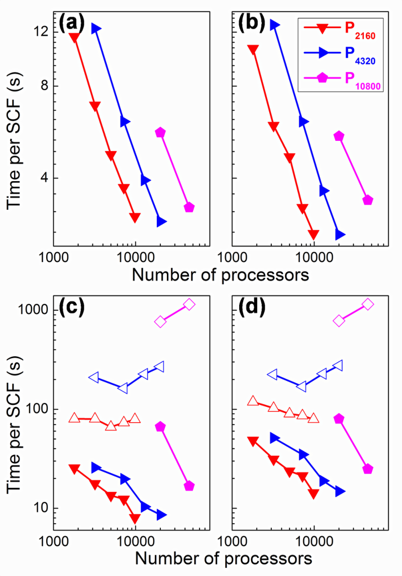
Fig. 3(c) and (d) show that the evaluation of the approximate charge density using the DG Hamiltonian matrix dominates the total wall clock time per SCF iteration in the DGDFT methodology. For large-scale ACPNRs, the PEXSI method can effectively reduce the wall clock time compared to the DIAG method in the DGDFT methodology. Furthermore, using the DIAG method with ScaLAPACK,20 appears to limit the strong parallel scalability for large-scale ACPNRs to at most 5,000 processors on the Edison. Increasing the number of processors beyond that can lead to an increase in wall clock time. In contrast, the PEXSI method exhibits highly scalable performance. It can make efficient use of more than 20,000-50,000 processors on Edison for . It should be noted that the total wall clock time required for performing large-scale ACPNRs containing thousands or tens of thousands of atoms is only about 10-25 seconds per SCF iteration.
4.3 AIMD simulation
Ab-initio molecular dynamics (AIMD) simulation capability has been implemented in the DGDFT method.44 We use DGDFT AIMD simulation to study the thermodynamic stability of ACPNRs. Using P180 as an example, we perform an AIMD simulation to obtain a 2.5 picosecond (ps) trajectory of ACPNR dynamics with a time step of 2.0 femtosecond (fs) under canonical ensemble with the temperature fixed at 300 K controlled by a single level Nose-Hoover thermostat.45, 46 The mass of the Nose-Hoover thermostat is chosen to be au. We use the GGA-PBE42 exchange-correlation functional for this particular simulation.
In Fig. 4, we plot the temperature (computed by where is the kinetic energy) and total free energy of P180 along the simulated trajectory. The temperature of the system reaches around K after ps. Although DGDFT only uses the Hellmann-Feynman force, we have observed that the drift of the conserved Hamiltonian in the Nose-Hoover thermostat is relatively small at Hartree per atom per ps.

We examine the electronic structures of P180 during 2.5 ps at 300 K as shown in Fig. 5. Geometric structures and density of states (DOS) of three AIMD snapshots at = 0.0, 0.6 and 2.0 ps are plotted in Fig. 5(b) and (c). In the initial configuration (t = 0.0 ps), the geometry of ACPNR is optimized first by using a gradient descent method with the Barzilai-Borwein line search technique47 implemented in DGDFT. After t = 0.6 ps, the ACPNR exhibits some local deformations due to the thermal perturbation introduced by the temperature. After t = 2.0 ps, 2 1 edge reconstruction can be observed. We find that the electronic structures of ACPNRs are also affected by thermal perturbation and edge reconstruction. Fig. 5 (a) indicates that the highest occupied molecular orbital (HOMO) energy is shifted by around eV, and the lowest unoccupied molecular orbital (LUMO) energy is shifted by around eV along the MD trajectory. The HOMO-LUMO energy gaps of P180 are calculated to be 0.63, 0.44 and 0.38 eV at = 0.0, 0.6 and 2.0 ps, respectively, showing that the shift of the energy level is more pronounced for the HOMO than the LUMO as shown in Fig. 5 (c). Therefore, the edge-unpassivated ACPNRs are also thermodynamically unstable just like the edge-unpassivated ZZPNRs.36, 37 This behavior is quite different from that of edge-unpassivated graphene nanoribbons.33, 34, 35 The reconstruction of edges in PNRs can modify their electronic36, 37 and transport38 properties and make them potential candidate materials for phosphorene-based electronic devices, such as field effect transistors.24

5 Conclusions
In summary, we developed a massively parallel DGDFT (Discontinuous Galerkin Density Functional Theory) methodology for efficient large-scale Kohn-Sham density functional theory (DFT) calculations based on the combination of the adaptive local basis (ALB) set and the pole expansion and selected inversion (PEXSI) technique. The DGDFT methodology can achieve a high basis set accuracy comparable to that provided by conventional plane wave calculations but with a small number of ALB basis functions per atom for large-scale electronic structure calculations that involve thousand or tens of thousands of atoms. Furthermore, the DGDFT methodology is highly scalable based on two levels of parallelization (intra- and inter-element parallelization), which can make efficient use of more than 50,000 processors on high performance machines for the systems studied here. Using ab-initio molecular dynamics calculations on armchair phosphorene nanoribbons (ACPNRs), we find that a 2 1 edge reconstruction appears in ACPNRs at room temperature to modify their electronic structures for phosphorene-based nanoelectronics in the future.
6 Acknowledgments
This work is partially supported by the Scientific Discovery through Advanced Computing (SciDAC) Program funded by U.S. Department of Energy, Office of Science, Advanced Scientific Computing Research and Basic Energy Sciences (W. H., L. L. and C. Y.), and by the Center for Applied Mathematics for Energy Research Applications (CAMERA), which is a partnership between Basic Energy Sciences and Advanced Scientific Computing Research at the U.S Department of Energy (L. L. and C. Y.). We thank the National Energy Research Scientific Computing (NERSC) center for the computational resources.
References
- 1 P. Hohenberg and W. Kohn, Phys. Rev., 1964, 136, B864.
- 2 W. Kohn and L. J. Sham, Phys. Rev., 1965, 140, B1133.
- 3 S. Goedecker, Rev. Mod. Phys., 1999, 71, 1085.
- 4 H. Shang, H. Xiang, Z. Li and J. Yang, Int. Rev. Phys. Chem., 2010, 29, 665–691.
- 5 D. R. Bowler and T. Miyazaki, Rep. Prog. Phys., 2012, 75, 036503.
- 6 J. M. Soler, E. Artacho, J. D. Gale, A. García, J. Junquera, P. Ordejón and D. Sánchez-Portal, J. Phys.: Condens. Matter, 2002, 14, 2745.
- 7 M. J. Gillan, D. R. Bowler, A. S. Torralba and T. Miyazaki, Comput. Phys. Commun., 2007, 177, 14–18.
- 8 T. Ozaki and H. Kino, Phys. Rev. B, 2005, 72, 045121.
- 9 X. Qin, H. Shang, H. Xiang, Z. Li and J. Yang, Int. J. Quantum Chem., 2014.
- 10 G. Kresse and J. Furthmüller, Phys. Rev. B, 1996, 54, 11169.
- 11 L. Lin, J. Lu, L. Ying and W. E, J. Comput. Phys., 2012, 231, 2140–2154.
- 12 L. Lin, J. Lu, L. Ying, R. Car and W. E, Comm. Math. Sci., 2009, 7, 755.
- 13 L. Lin, M. Chen, C. Yang and L. He, J. Phys.: Condens. Matter, 2013, 25, 295501.
- 14 L. Lin, A. García, G. Huhs and C. Yang, J. Phys.: Condens. Matter, 2014, 26, 305503.
- 15 D. N. Arnold, SIAM J. Numer. Anal., 1982, 19, 742–760.
- 16 D. N. Arnold, F. Brezzi, B. Cockburn and L. D. Marini, SIAM J. Numer. Anal., 2002, 39, 1749–1779.
- 17 A. V. Knyazev, SIAM J. Sci. Comp., 2001, 23, 517–541.
- 18 J. Kaye, L. Lin and C. Yang, Comm. Math. Sci., 2015, accepted, .
- 19 W. Hu, L. Lin, C. Yang and J. E. Pask, in preparation, 2015.
- 20 T. Auckenthaler, V. Blum, H. J. Bungartz, T. Huckle, R. Johanni, L. Krämer, B. Lang, H. Lederer and P. R. Willems, Parallel Comput., 2011, 37, 783–794.
- 21 W. Hu, L. Lin, C. Yang and J. Yang, J. Chem. Phys., 2014, 141, 214704.
- 22 H. Liu, A. T. Neal, Z. Zhu, Z. Luo, X. Xu, D. Tománek and P. D. Ye, ACS Nano, 2014, 8, 4033–4041.
- 23 J. Qiao, X. Kong, Z.-X. Hu, F. Yang and W. Ji, Nature Commun., 2014, 5, 4475.
- 24 L. Li, Y. Yu, G. Ye, Q. Ge, X. Ou, H. Wu, D. Feng, X. Chen and Y. Zhang, Nature Nanotech., 2014, 9, 372–377.
- 25 J. Dai and X. C. Zeng, J. Phys. Chem. Lett., 2014, 5, 1289–1293.
- 26 K. S. Novoselov, A. K. Geim, S. V. Morozov, D. Jiang, Y. Zhang, S. V. Dubonos, I. V. Grigorieva and A. A. Firsov, Scinece, 2004, 306, 666–669.
- 27 A. K. Geim and K. S. Novoselov, Nature Mater., 2007, 6, 183–191.
- 28 A. H. C. Neto, F. Guinea, N. M. R. Peres, K. S. Novoselov and A. K. Geim, Rev. Mod. Phys., 2009, 18, 109.
- 29 G. Andrew, Science News, 2014, 185, 13.
- 30 E. V. Castro, K. S. Novoselov, S. V. Morozov, N. M. R. Peres, J. M. B. L. dos Santos, J. Nilsson, F. Guinea, A. K. Geim and A. H. C. Neto, Phys. Rev. Lett., 2007, 99, 216802.
- 31 F. Schedin, A. K. Geim, S. V. Morozov, E. W. Hill, P. Blake, M. I. Katsnelson and K. S. Novoselov, Nature Mater., 2007, 6, 652–655.
- 32 S. Y. Zhou, G.-H. Gweon, A. V. Fedorov, P. N. First, W. A. de Heer, D.-H. Lee, F. Guinea, A. H. C. Neto and A. Lanzara, Nature Mater., 2007, 6, 770–775.
- 33 V. Barone, O. Hod and G. E. Scuseria, Nano Lett., 2006, 6, 2748–2754.
- 34 Y.-W. Son, M. L. Cohen and S. G. Louie, Phys. Rev. Lett., 2006, 97, 216803.
- 35 L. Yang, C.-H. Park, Y.-W. Son, M. L. Cohen and S. G. Louie, Phys. Rev. Lett., 2007, 99, 186801.
- 36 A. Ramasubramaniam and A. R. Muniz, Phys. Rev. B, 2014, 90, 085424.
- 37 H. Guo, N. Lu, J. Dai, X. Wu and X. C. Zeng, J. Phys. Chem. C, 2014, 118, 14051–14059.
- 38 L. Kou, T. Frauenheim and C. Chen, J. Phys. Chem. Lett., 2014, 5, 2675–2681.
- 39 X. Han, H. M. Stewart, S. A. Shevlin, C. R. A. Catlow and Z. X. Guo, Nano Lett., 2014, 14, 4607–4614.
- 40 X. Gonze, B. Amadon, P.-M. Anglade, J.-M. Beuken, F. Bottin, P. Boulanger, D. C. F. Bruneval, R. Caracas, M. Côté, T. Deutsch, L. Genovese, P. Ghosez, M. Giantomassi, S. Goedecker, D. R. Hamann, P. Hermet, F. Jollet, G. Jomard, S. Leroux, M. Mancini, S. Mazevet, M. J. T. Oliveira, G. Onida, Y. Pouillon, T. Rangel, G.-M. Rignanese, D. Sangalli, R. Shaltaf, M. Torrent, M. J. Verstraete, G. Zerah and J. W. Zwanziger, Comput. Phys. Commun., 2009, 180, 2582–2615.
- 41 S. Goedecker, M. Teter and J. Hutter, Phys. Rev B, 1996, 54, 1703.
- 42 J. P. Perdew, K. Burke and M. Ernzerhof, Phys. Rev. Lett., 1996, 77, 3865.
- 43 C. Hartwigsen, S. Goedecker and J. Hutter, Phys. Rev B, 1998, 58, 3641.
- 44 G. Zhang, L. Lin, W. Hu, C. Yang and J. E. Pask, in preparation, 2015.
- 45 S. Nosé, J. Chem. Phys., 1984, 81, 511.
- 46 W. G. Hoover, Phys. Rev. A, 1985, 31, 1695.
- 47 R. Fletcher, Springer US, 2005, 96, 235–256.