Optimized Uplink Transmission in Multi-Antenna C-RAN with Spatial Compression and Forward

It is anticipated that the mobile data traffic will grow 1000 times higher in the next decade with a rate of roughly a factor of two per year [1]. As a result, the fifth-generation or 5G wireless system on the roadmap has to make a major paradigm shift to accommodate this dramatic explosion in future demands for wireless data communications. Both as highly promising candidate techniques for the 5G wireless network, massive multiple-input multiple-output (MIMO) [2, 3] and cloud radio access network (C-RAN) [4] have recently drawn significant attentions (see Fig. 1). Both techniques advocate the use of very large number of antennas and centralized signal processing to achieve enormously improved efficiency in spectrum and energy usage. However, they are practically implemented with different performance and complexity trade-off considerations.

In a massive MIMO system, as depicted in Fig. 1(a), a large number of antennas are deployed at the base station (BS) to reap all the benefits of the conventional multi-user MIMO system but with a much greater scale. It is shown in [2] that in the asymptotic regime where the number of antennas at the BS is much larger than that of the users, the channels of different users are orthogonal with each other, and thus a simple matched filter, i.e., maximal ratio combining (MRC) in the uplink and maximal ratio transmission (MRT) in the downlink, is capacity-achieving. Moreover, the required transmit energy per bit vanishes as the number of antennas goes to infinity [5]. Despite of the above appealing benefits, there are many issues that potentially limit the performance of massive MIMO. For instance, due to the limited space for installation, the number of antennas at the BS is finite and their channels are generally correlated; as a result, the theoretical performance limit in the asymptotic regime cannot be fully achieved in practice with simple MRC/MRT. Moreover, similar to conventional MIMO system, the performance of the cell-edge users in the massive MIMO system is still a bottleneck since their channel conditions may be weak due to more significant path attenuation.

On the other hand, in a single-antenna C-RAN as shown in Fig. 1(b), each antenna is deployed at one separate site called remote radio head (RRH), which is connected to one central unit (CU) via a high-speed fronthaul link (fiber or wireless) for joint information processing. Unlike the BS in the massive MIMO system which decodes or encodes the user messages locally, in C-RAN each RRH merely forwards the signals to/from the CU via its fronthaul link, while leaving the joint encoding/decoding complexity to a baseband unit (BBU) in the CU. As a result, if the data can be perfectly transmitted between the BBU and RRHs over the fronthaul links without any error, the single-antenna C-RAN can be viewed as another form of massive MIMO but with the antennas densely distributed over the whole served region such that all the mobile users can be served by some adjacent antennas with strong channel conditions. However, one obstacle constraining the practically achievable throughput of C-RAN is the limited-capacity fronthaul link between each RRH and BBU. According to [4], the capacity of the current commercial fibers, which is about several Gbps (gigabits per second), can be easily overwhelmed in C-RAN even under moderate data traffic; whereas wireless fronthaul techniques such as those exploiting the millimeter-wave bands in general operate with even lower data rate per link and shorter distance as compared to the fiber based solution. In the literature, a considerable amount of effort has been dedicated to study fronthaul quantization/compression techniques in the uplink communication [6]-[12]. Specifically, the “quantize-and-forward (QF)” scheme [13]-[15] is adopted to reduce the communication rates between the BBU and RRHs, where each single-antenna RRH samples, quantizes and forwards its received signals to the BBU over its fronthaul link. Moreover, the QF scheme is usually studied under an information-theoretical Gaussian test channel model, and the quantization noise levels of all the RRHs are jointly optimized to maximize the end-to-end throughput subject to the capacity constraints of individual fronthaul links. Recently, [16] reveals that subject to the capacity of the current commercial fibers, the above theoretical performance upper bound can be approached by applying a simple uniform scalar quantization at each RRH for orthogonal frequency division multiplexing (OFDM) based single-antenna C-RAN. Moreover, another line of research in C-RAN studies the control of the overall fronthaul traffic by selectively activating only a small subset of all the RRHs to meet the user demands [17].

In the aforementioned massive MIMO system and single-antenna C-RAN, the antennas are deployed in a totally co-located and separated manner, respectively. In addition to these two extreme cases, a more general solution is to distribute the antennas at a reduced number of sites as compared to single-antenna C-RAN, while the RRH at each site is equipped with multiple antennas. This so-called multi-antenna C-RAN design can provide both improved channel conditions to the users as in single-antenna C-RAN as well as local spatial multiplexing gain as in massive MIMO; furthermore, by adjusting the number of antennas at each RRH and the number of RRHs, these benefits can be flexibly traded-off with a given total number of antennas deployed. However, the fronthaul issue becomes more severe in the multi-antenna C-RAN as compared to conventional single-antenna counterpart, since the limited fronthaul capacity at each RRH needs to be allocated over the outputs of more antennas, thus leading to more quantization errors in general. To tackle this challenge and address the above design trade-off, in this paper we focus our study on the uplink communication in C-RAN with multi-antenna RRHs each subject to a finite fronthaul capacity constraint. The contributions of this paper are summarized as follows.

• •

  We propose a novel “spatial-compression-and-forward (SCF)” scheme for the multi-antenna RRHs to balance between the information conveyed to the BBU and the data traffic over the fronthaul links. Specifically, each RRH first performs spatial filtering to its received signals at different antennas from the users such that the signals are denoised and maximally compressed into a reduced number of dimensions. Then, the RRH applies the simple uniform scalar quantization [16] over each of these dimensions in parallel by appropriately allocating the number of quantization bits over them under a total rate constraint. Last, the quantized bits by RRHs are sent to the BBU for joint information decoding via their fronthaul links. It is worth noting that at each RRH, the compression of the correlated signals received by all its antennas is fulfilled by a simple linear filter, rather than the complicated distributed source coding, e.g., Wyner-Ziv coding, as in single-antenna C-RAN where all the antennas are physically separated [11, 12].

• •

  With the proposed SCF scheme, we formulate the optimization problem of joint users’ power allocation, RRHs’ spatial filter design and quantization bits allocation, as well as BBU’s receive beamforming to maximize the minimum signal-to-interference-plus-noise ratio (SINR) of all the users in the uplink. We propose an efficient solution to this complicated design problem for ease of practical implementation. First, each RRH computes its own spatial filter in a distributed manner based on its locally received signal covariance matrix. This distributed solution helps save significant fronthaul resources for exchanging control signals with the BBU. Then, the BBU jointly optimizes the other parameters to maximize the minimum SINR of all users based on the alternating optimization technique. Specifically, with given quantization bits allocation at each RRH, we extend the well-known fixed-point method [18] to obtain the optimal transmit power levels for the users and receive beamforming vectors at the BBU. On the other hand, given the above optimized parameters, the corresponding quantization bits allocation at each RRH is efficiently solved.

• •

  Last, we investigate the following interesting question: Given a total number of antennas for a target area, should all of them be deployed at one BS, i.e., massive MIMO, or one at each RRH, i.e., single-antenna C-RAN, or optimally divided over a certain number of RRHs, i.e., multi-antenna C-RAN, given a practical total fronthaul capacity constraint for C-RAN? Through numerical examples, it is shown that with the proposed SCF scheme and joint wireless-fronthaul-BBU optimization, multi-antenna C-RAN generally performs noticeably better than both massive MIMO and single-antenna C-RAN under moderate fronthaul rate constraints.

The rest of this paper is organized as follows. Section II presents the system model for C-RAN with the SCF scheme. Section III formulates the minimum SINR maximization problem. Section IV presents the proposed solution for this problem. Section V provides numerical results to verify the effectiveness of the proposed multi-antenna C-RAN with SCF. Finally, Section VI concludes the paper.

Notation: Scalars are denoted by lower-case letters, vectors by bold-face lower-case letters, and matrices by bold-face upper-case letters. $I$ and $0$ denote an identity matrix and an all-zero matrix, respectively, with appropriate dimensions. For a square matrix $S$, $\mbox{\boldmath{$S$}}\succeq\mbox{\boldmath{$0$}}$ ($\mbox{\boldmath{$S$}}\preceq\mbox{\boldmath{$0$}}$) means that $S$ is positive (negative) semi-definite. For a matrix $M$ of arbitrary size, $\mbox{\boldmath{$M$}}^{H}$ and ${\rm rank}(\mbox{\boldmath{$S$}})$ denote the conjugate transpose and rank of $M$, respectively. ${\rm diag}(\mbox{\boldmath{$a$}})$ denotes a diagonal matrix with the main diagonal given by the vector $a$, while ${\rm diag}(\mbox{\boldmath{$A$}}_{1},\cdots,\mbox{\boldmath{$A$}}_{K})$ denotes a block diagonal matrix with the diagonal given by square matrices $\mbox{\boldmath{$A$}}_{1},\cdots,\mbox{\boldmath{$A$}}_{K}$. $E[\cdot]$ denotes the statistical expectation. The distribution of a circularly symmetric complex Gaussian (CSCG) random vector with mean $x$ and covariance matrix $\Sigma$ is denoted by $\mathcal{CN}(\mbox{\boldmath{$x$}},\mbox{\boldmath{$\Sigma$}})$; and $\sim$ stands for “distributed as”. $\mathbb{C}^{x\times y}$ denotes the space of $x\times y$ complex matrices. $\|\mbox{\boldmath{$x$}}\|$ denotes the Euclidean norm of a complex vector $x$. For two real vectors $x$ and $y$, $\mbox{\boldmath{$x$}}\geq\mbox{\boldmath{$y$}}$ means that $x$ is greater than or equal to $y$ in a component-wise manner.

This paper considers the uplink communication in a multi-antenna C-RAN. As shown in Fig. 1(c), the system consists of one BBU, $N$ RRHs, denoted by the set $\mathcal{N}=\{1,\cdots,N\}$, and $K$ users, denoted by the set $\mathcal{K}=\{1,\cdots,K\}$. It is assumed that each RRH is equipped with $M\geq 1$ antennas, while each user is equipped with one single antenna. It is further assumed that each RRH $n$ is connected to the BBU via a digital error-free fronthaul link with a capacity of $\bar{T}_{n}$ bits per second (bps). In the uplink, each RRH processes the signals received from all the users into digital bits and forwards them to the BBU via its fronthaul link. Then, the BBU jointly decodes the users’ messages based on the signals from all the RRHs. The details of our studied uplink multi-antenna C-RAN are given as follows.

It is assumed that all the $K$ users transmit over quasi-static flat-fading channels over a given bandwidth of $B$ Hz.¹¹ 1 It is worth noting that this paper studies the narrowband wireless channel, while the results obtained can be readily extended to broadband based C-RAN by viewing each frequency subchannel as one norrowband channel considered here and accordingly scaling down the fronthaul capacity $\bar{T}_{n}$ by the number of frequency subchannels in use. The equivalent baseband complex symbol received at RRH $n$ is then expressed as

where $\mbox{\boldmath{$s$}}=[s_{1},\cdots,s_{K}]^{T}$ with $s_{k}\sim\mathcal{CN}(0,1)$ denoting the transmit symbol of user $k$ which is modelled as a CSCG random variable with zero-mean and unit-variance, $\mbox{\boldmath{$P$}}={\rm diag}(p_{1},\cdots,p_{K})$ with $p_{k}$ denoting the transmit power of user $k$, $\mbox{\boldmath{$H$}}_{n}=[\mbox{\boldmath{$h$}}_{n,1},\cdots,\mbox{\boldmath{$h$}}_{n,K}]\in\mathbb{C}^{M\times K}$ with $\mbox{\boldmath{$h$}}_{n,k}\in\mathbb{C}^{M\times 1}$ denoting the channel vector from user $k$ to RRH $n$, and $\mbox{\boldmath{$z$}}_{n}\sim\mathcal{CN}(\mbox{\boldmath{$0$}},\sigma_{n}^{2}\mbox{\boldmath{$I$}})$ denotes the additive white Gaussian noise (AWGN) at RRH $n$. It is assumed that $\mbox{\boldmath{$z$}}_{n}$’s are independent over $n$.

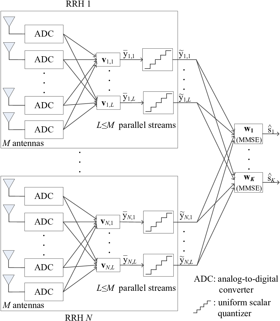
At each multi-antenna RRH, we consider the use of the SCF scheme to forward the received baseband symbol $\mbox{\boldmath{$y$}}_{n}$ to the BBU via the finite-capacity digital fronthaul link. An illustration of the SCF scheme is shown in Fig. 2, where each RRH first demodulates the signal received from each antenna to the baseband and processes the baseband signals from all antennas via spatial filtering, then conducts a scalar quantization over each output in parallel, and finally forwards the total quantized bits to the BBU via the fronthaul link. Specifically, RRH $n$ first implements spatial filtering to its received signal $\mbox{\boldmath{$y$}}_{n}$ to obtain

where $\mbox{\boldmath{$V$}}_{n}=[\mbox{\boldmath{$v$}}_{n,1},\cdots,\mbox{\boldmath{$v$}}_{n,L}]^{T}\in\mathbb{C}^{L\times M}$ denotes the filtering matrix at RRH $n$ with $L\leq M$ denoting the (reduced) dimension of the output signal $\bar{\mbox{\boldmath{$y$}}}_{n}$ after filtering, which will be specified later. Then, a simple uniform scalar quantization is applied to each element of $\bar{\mbox{\boldmath{$y$}}}_{n}=[\bar{y}_{n,1},\cdots,\bar{y}_{n,L}]^{T}$ at RRH $n$. Note that each complex symbol $\bar{y}_{n,l}$ can be represented by its in-phase (I) and quadrature (Q) parts as

where $j^{2}=-1$, and the I-branch symbol $\bar{y}_{n,l}^{I}$ and Q-branch symbol $\bar{y}_{n,l}^{Q}$ are both real Gaussian random variables with zero mean and variance $(\sum_{k=1}^{K}p_{k}|\mbox{\boldmath{$v$}}_{n,l}^{T}\mbox{\boldmath{$h$}}_{n,k}|^{2}+\sigma^{2}\|\mbox{\boldmath{$v$}}_{n,l}\|^{2})/2$. A typical method to implement the uniform quantization is via separate I/Q scalar quantization, the details of which can be found in [16]. After uniform scalar quantization, the baseband quantized symbol of $\bar{\mbox{\boldmath{$y$}}}_{n}$ is then given by

where $\mbox{\boldmath{$e$}}_{n}=[e_{n,1},\cdots,e_{n,L}]^{T}$ with $e_{n,l}$, $1\leq l\leq L$, denoting the quantization error for $\bar{y}_{n,l}$ with zero mean and variance $q_{n,l}$. Let $D_{n,l}$ denote the number of bits that RRH $n$ uses to quantize the I-branch or Q-branch of $\bar{y}_{n,l}$, i.e., $\bar{y}_{n,l}^{I}$ or $\bar{y}_{n,l}^{Q}$. The quantization noise level $q_{n,l}$ due to $e_{n,l}$ for uniform quantization is then given by [16]

Note that $e_{n,l}$’s are independent over $l$ due to independent scalar quantization for each element of $\bar{\mbox{\boldmath{$y$}}}_{n}$, and also over $n$ due to independent processing at different RRHs. As a result, the covariance matrix of $\mbox{\boldmath{$e$}}_{n}$ is a function of $\mbox{\boldmath{$p$}}=[p_{1},\cdots,p_{K}]^{T}$, $\mbox{\boldmath{$V$}}_{n}$ as well as $\mbox{\boldmath{$D$}}_{n}=[D_{n,1},\cdots,D_{n,L}]^{T}$, which is given by

Then, each RRH forwards the quantized bits to the BBU via the fronthaul link. The transmission rate in RRH $n$’s fronthaul link is expressed as [16]

It is worth noting that if $D_{n,l}=0$, then the symbol $\bar{y}_{n,l}$ at the spatial filter output dimension $l$ is not quantized at RRH $n$ and thus not forwarded to the BBU; as a result, $q_{n,l}=\infty$ according to (II). To summarize, our proposed SCF scheme is a two-stage compression method, where the output signal dimension at each RRH is first reduced from $M$ to $L$ (if $M>L$) by spatial filtering, and then further reduced by allocating the limited fronthaul quantization bits to only a selected subset of the $L$ output dimensions with $D_{n,l}>0$.

The received signal at the BBU from all RRHs is expressed as

where $\mbox{\boldmath{$V$}}={\rm diag}(\mbox{\boldmath{$V$}}_{1},\cdots,\mbox{\boldmath{$V$}}_{N})$, $\mbox{\boldmath{$h$}}_{(k)}=[\mbox{\boldmath{$h$}}_{1,k}^{T},\cdots,\mbox{\boldmath{$h$}}_{N,k}^{T}]^{T}$, $\mbox{\boldmath{$z$}}=[\mbox{\boldmath{$z$}}_{1}^{T},\cdots,\mbox{\boldmath{$z$}}_{N}^{T}]^{T}$, and $\mbox{\boldmath{$e$}}=[\mbox{\boldmath{$e$}}_{1}^{T},\cdots,\mbox{\boldmath{$e$}}_{N}^{T}]^{T}$. To decode $s_{k}$, we consider that a linear beamforming²² 2 It is worth noting that the subsequent results also hold similarly for the case with the non-linear successive interference cancellation scheme with any fixed decoding order, which is not considered in this paper due to its high complexity for implementation. is applied to $\tilde{\mbox{\boldmath{$y$}}}$, i.e.,

where $\mbox{\boldmath{$w$}}_{k}=[w_{k,1},\cdots,w_{k,NL}]^{T}\in\mathbb{C}^{NL\times 1}$ is the receive beamformer for $s_{k}$. Note that $w_{k,(n-1)L+l}=0$ if the $l$th signal dimension at RRH $n$ is not quantized, i.e., $D_{n,l}=0$. According to (10), the SINR for decoding $s_{k}$ is expressed as

where $\mbox{\boldmath{$Q$}}(\mbox{\boldmath{$p$}},\{\mbox{\boldmath{$V$}}_{n},\mbox{\boldmath{$D$}}_{n}\})=E[\mbox{\boldmath{$e$}}\mbox{\boldmath{$e$}}^{H}]={\rm diag}(\mbox{\boldmath{$Q$}}_{1}(\mbox{\boldmath{$p$}},\mbox{\boldmath{$V$}}_{1},\mbox{\boldmath{$D$}}_{1}),\cdots,\mbox{\boldmath{$Q$}}_{N}(\mbox{\boldmath{$p$}},\mbox{\boldmath{$V$}}_{N},\mbox{\boldmath{$D$}}_{N}))$.

In this paper, we aim to maximize the minimum SINR of all the users by optimizing the users’ power allocation, i.e., $p$, the spatial filter and quantization bits allocation at each RRH, i.e., $\mbox{\boldmath{$V$}}_{n}$ and $\mbox{\boldmath{$D$}}_{n}$, $\forall n$, and the receive beamforming vectors at the BBU, i.e., $\mbox{\boldmath{$w$}}_{k}$, $\forall k$. Specifically, we aim to solve the following problem:

where $\gamma$ denotes the common SINR target for all the $K$ users and $\bar{P}_{k}$ denotes the transmit power constraint of user $k$.

It can be observed that problem (12) is a non-convex optimization problem since the design variables are complicatedly coupled in its constraint (13). Note that with given $\mbox{\boldmath{$V$}}_{n}$’s and by setting $D_{n,l}=\infty$, $\forall n,l$, problem (12) reduces to the well-known SINR balancing problem via transmit power control and receive beamforming only. This problem has been efficiently solved by [19, 20] based on the non-negative matrix theory [21]. However, due to the new quantization noise term in the SINR expression, i.e., $\mbox{\boldmath{$w$}}_{k}^{H}\mbox{\boldmath{$Q$}}(\mbox{\boldmath{$p$}},\{\mbox{\boldmath{$V$}}_{n},\mbox{\boldmath{$D$}}_{n}\})\mbox{\boldmath{$w$}}_{k}$, it can be shown that the algorithm proposed in [19, 20] cannot be directly applied to obtain the optimal power control and beamforming solution to problem (12) even with given $\mbox{\boldmath{$V$}}_{n}$’s and finite values of $D_{n,l}$’s. As a result, with the additional variables $\mbox{\boldmath{$V$}}_{n}$’s and integer variables $\mbox{\boldmath{$D$}}_{n}$’s, it is generally difficult to globally solve problem (12).

In this paper, we propose an efficient algorithm to solve problem (12) suboptimally, for which the main procedures are illustrated in Fig. 3. Specifically, in the channel training phase, all the users send orthogonal pilot signals to the RRHs with equal power $\bar{P}\leq\min_{1\leq k\leq K}\bar{P}_{k}$. Let $\mbox{\boldmath{$y$}}_{pilot,n}\in\mathbb{C}^{M\times 1}$ denote the received signal at RRH $n$ during the channel training phase. Then, each RRH $n$ estimates the MIMO channel $\mbox{\boldmath{$H$}}_{n}$ (assumed to be perfect) and computes the covariance matrix of its received signal (with the presumed knowledge of $\bar{P}$ and $\sigma^{2}$), i.e.,

Then each RRH independently determines its spatial filter $\mbox{\boldmath{$V$}}_{n}$ based on $\mbox{\boldmath{$S$}}_{n}$. Next, each RRH $n$ sends the effective channel $\mbox{\boldmath{$V$}}_{n}\mbox{\boldmath{$H$}}_{n}\triangleq\tilde{\mbox{\boldmath{$H$}}}_{n}=[\tilde{\mbox{\boldmath{$h$}}}_{n,1},\cdots,\tilde{\mbox{\boldmath{$h$}}}_{n,K}]$ to the BBU. Then, based on its global CSI, i.e., $\tilde{\mbox{\boldmath{$H$}}}_{n}$’s, $n=1,\cdots,N$, the BBU computes $p$, $\mbox{\boldmath{$D$}}_{n}$’s and $\mbox{\boldmath{$w$}}_{k}$’s by solving the following reduced problem of problem (12):

where $\tilde{\mbox{\boldmath{$h$}}}_{(k)}=[\tilde{\mbox{\boldmath{$h$}}}_{1,k}^{T},\cdots,\tilde{\mbox{\boldmath{$h$}}}_{N,k}^{T}]^{T}$. Finally, the BBU sends $\mbox{\boldmath{$D$}}_{n}$ to RRH $n$, $n=1,\cdots,N$, via its fronthaul link for the implementation of scalar quantization, and $p$ to one RRH (say RRH $n$), which then broadcasts $p$ to all the users in the downlink. In the following section, we first show how each RRH computes its spatial filter in a distributed manner, and then discuss how the BBU solves problem (18).

In this section, we present details of the two-stage algorithm for solving problem (12) based on the diagram shown in Fig. 3.

References

- [1] 3GPP, “Report of 3GPP RAN Workshop on Release 12 and onwards,” RWS- 120052, 3GPP Workshop on Release 12 Onward, June 2012.
- [2] T. L. Marzetta, “Noncooperative cellular wireless with unlimited numbers of base station antennas,” IEEE Trans. Wireless Commun., vol. 9, no. 11, pp. 3590¨C3600, Nov. 2010.
- [3] L. Lu, G. Y. Li, A. L. Swindlehurst, A. Ashikhmin, and R. Zhang, “An overview of massive MIMO: benefits and challenges,” IEEE J. Sel. Topics Signal Process., vol. 8, no. 5, pp. 742-758, Oct. 2014.
- [4] “C-RAN: the road towards green RAN,” China Mobile Res. Inst., Beijing, China, Oct. 2011, White Paper, ver. 2.5.
- [5] H. Q. Ngo, E. G. Larsson, and T. L. Marzetta, ”Energy and spectral efficiency of very large multiuser MIMO systems,” IEEE Trans. Commun., vol. 61, no. 4, pp. 1436¨C1449, Apr. 2013.
- [6] A. Sanderovich, S. Shamai, and Y. Steinberg, “Distributed MIMO receiver - Achievable rates and upper bounds,” IEEE Trans. Inf. Theory, vol. 55, no. 10, pp. 4419-4438, Oct. 2009.
- [7] A. Sanderovich, O. Somekh, H. V. Poor, and S. Shamai (Shitz), “Uplink macro diversity of limited backhaul cellular network,” IEEE Trans. Inf. Theory, vol. 55, no. 8, pp. 3457-3478, Aug. 2009.
- [8] S. H. Park, O. Simeone, O. Sahin, and S. Shamai, “Joint decompression and decoding for cloud radio access networks,” IEEE Signal Processing Letters, vol. 20, no. 5, pp. 503-506, May 2013.
- [9] A. D. Coso and S. Simoens, “Distributed compression for MIMO coordinated networks with a backhaul constraint,” IEEE Trans. Wireless Commun., vol. 8, no. 9, pp. 4698-4709, Sep. 2009.
- [10] S. H. Park, O. Simeone, O. Sahin, and S. Shamai, “Robust and efficient distributed compression for cloud radio access networks,” IEEE Trans. Vehicular Technology, vol. 62, no. 2, pp. 692-703, Feb. 2013.
- [11] Y. Zhou and W. Yu, “Optimized backhaul compression for uplink cloud radio access network,” IEEE J. Sel. Areas Commun., vol. 32, no. 6, pp. 1295-1307, June 2014.
- [12] L. Zhou and W. Yu, “Uplink multicell processing with limited backhaul via per-base-station successive interference cancellation,” IEEE J. Sel. Areas Commun., vol. 30, no. 10, pp. 1981-1993, Oct. 2013.
- [13] A. Avestimehr, S. Diggavi, and D. Tse, “Wireless network information flow: A deterministic approach,” IEEE Trans. Inf. Theory, vol. 57, no. 4, pp. 1872-1905, Apr. 2011.
- [14] S. H. Lim, Y. H. Kim, A. El Gamal, and S. Y. Chung, “Noisy network coding,” IEEE Trans. Inf. Theory, vol. 57, no. 5, pp. 3132-3152, May 2011.
- [15] A. Sanderovich, S. Shamai, Y. Steinberg, and G. Kramer, “Communication via decentralized processing,” IEEE Trans. Inf. Theory, vol. 54, no. 7, pp. 3008-3023, July 2008.
- [16] L. Liu, S. Bi, and R. Zhang, “Joint power control and fronthaul rate allocation for throughput maximization in OFDMA-based cloud radio access network,” submitted to IEEE Trans. Wireless Commun.. (Available on-line at arXiv:1407.3855)
- [17] S. Luo, R. Zhang, and T. J. Lim, “Downlink and uplink energy minimization through user association and beamforming in cloud RAN,” IEEE Trans. Wireless Commun., vol. 14, no. 1, pp. 494-508, Jan. 2015.
- [18] R. D. Yates, “A framework for uplink power control in cellular radio systems,” IEEE J. Select. Areas Commun., vol. 13, pp. 1341-1347, Sept. 1995.
- [19] M. Schubert and H. Boche, “Solution of the multiuser downlink beamforming problem with individual SINR constraints,” IEEE Trans. Veh. Technol., vol. 53, no. 1, pp. 18-28, Jan. 2004.
- [20] L. Zhang, Y. C. Liang, and Y. Xin, “Joint beamforming and power control for multiple access channels in cognitive radio networks,” IEEE J. Sel. Areas Commun., vol. 26, no. 1, pp. 38-51, Jan. 2008.
- [21] R. Horn and C. Johnson, Matrix Analysis, Cambridge University Press, 1985.
- [22] M. Gastpar, P. L. Dragotti, and M. Vetterli, “The distributed Karhunen-Loeve transform,” IEEE Trans. Inf. Theory, vol. 52, no. 12, pp. 5171-5196, Dec. 2006.
- [23] I. D. Schizas, G. B. Giannakis, and Z. Q. Luo, “Distributed estimation using reduced-dimensionality sensor observations,” IEEE Trans. Signal Process., vol. 55, no. 8, pp. 4284-4299, Aug. 2007.
- [24] S. Boyd and L. Vandenberghe, Convex Optimization, Cambidge Univ. Press, 2004.