跳到论文正文
W Papers独立论文阅读器 arXiv:1501.04651 论文正文 计算阅读时间 · 0%
引用这篇论文根据当前论文元数据生成,正式投稿前建议核对。


License: arXiv.org perpetual non-exclusive license
arXiv:1501.04651v3 [hep-th] 03 Jun 2015

A Riemann-Hilbert formulation for the finite temperature Hubbard model

Andrea Cavaglià    Martina Cornagliotto Affiliation: Dipartimento di Fisica and INFN, Università di Torino, Via P. Giuria 1, 10125 Torino, Italy
DESY Hamburg, Theory Group, Notkestrasse 85, D-22607 Hamburg, Germany
cavaglia/mattelli/tateo@to.infn.it, martina.cornagliotto@desy.de
   Massimo Mattelliano    Roberto Tateo
Abstract: 

Inspired by recent results in the context of AdS/CFT integrability, we reconsider the Thermodynamic Bethe Ansatz equations describing the 1D fermionic Hubbard model at finite temperature. We prove that the infinite set of TBA equations are equivalent to a simple nonlinear Riemann-Hilbert problem for a finite number of unknown functions. The latter can be transformed into a set of three coupled nonlinear integral equations defined over a finite support, which can be easily solved numerically. We discuss the emergence of an exact Bethe Ansatz and the link between the TBA approach and the results by Jüttner, Klümper and Suzuki based on the Quantum Transfer Matrix method. We also comment on the analytic continuation mechanism leading to excited states and on the mirror equations describing the finite-size Hubbard model with twisted boundary conditions.

1 Introduction

The Hubbard model [1] arises as an approximate description of correlated electrons in narrow-band materials. Despite its simplicity, it is believed to capture important nonperturbative features of real many-body fermionic systems. In one dimension, the model is exactly solvable and its relevance for the study of strongly correlated electrons is perhaps comparable to that of the Ising model for magnetism. Quite unexpectedly, the Hubbard model has also attracted the attention of high energy physicists due to its multiple connections [2, 3, 4, 5, 6, 7, 8] with the integrable spin chains emerging in the context of 𝒩=4\mathcal{N}{=}4 Super Yang-Mills theory [9, 10, 11]. In particular, the exact Bethe Ansatz equations of Lieb and Wu [12], and the corresponding string hypothesis [13], have many features in common with the asymptotic Bethe Ansatz of Beisert and Staudacher for the anomalous dimensions of single-trace operators with large quantum numbers [11].

We start from the 1D Hubbard Hamiltonian written in the form

H0=−∑i=1L∑σ=↑,↓(ci,σ†ci+1,σ+ci+1,σ†ci,σ)+𝐮∑i=1L(1−2ci,↑†ci,↑)(1−2ci,↓†ci,↓),H_{0}=-\,\sum_{i=1}^{L}\sum_{\sigma=\uparrow,\downarrow}\left(c^{\dagger}_{i,\sigma}c_{i+1,\sigma}+c^{\dagger}_{i+1,\sigma}c_{i,\sigma}\right)+{\bf u}\,\sum_{i=1}^{L}(1-2\,c^{\dagger}_{i,\uparrow}c_{i,\uparrow})(1-2\,c^{\dagger}_{i,\downarrow}c_{i,\downarrow}), (1)

where LL is the length of the chain, ci,σ†c^{\dagger}_{i,\sigma} and ci,σc_{i,\sigma} are fermionic creation-annihilation operators satisfying

{ci,σ,cj,τ}={ci,σ†,cj,τ†}=0,{ci,σ,cj,τ†}=δi​j​δσ​τ,\displaystyle\{c_{i,\sigma},c_{j,\tau}\}=\{c^{\dagger}_{i,\sigma},c^{\dagger}_{j,\tau}\}=0,\,\,\,\,\{c_{i,\sigma},c^{\dagger}_{j,\tau}\}=\delta_{ij}\,\delta_{\sigma\tau}, (2)

with periodic boundary conditions c1,σ=cL+1,σc_{1,\sigma}=c_{L+1,\sigma}, c1,σ†=cL+1,σ†c^{\dagger}_{1,\sigma}=c^{\dagger}_{L+1,\sigma}, and 𝐮≥0{\bf u}\geq 0 is a dimensionless coupling constant proportional to the electric charge. For LL even, the Hamiltonian (1) is S​O​(4)SO(4)-symmetric [14]. We shall consider a two-parameter deformation of (1) where this symmetry is explicitly broken by coupling the electrons to a chemical potential μ\mu and to a magnetic field BB:

Hμ,B=H0−μ​N^−2​B​Sz,\displaystyle H_{\mu,B}=H_{0}-\mu{\hat{N}}-2BS^{z}, (3)

with the conserved electron number N^{\hat{N}} and spin SzS^{z} operators defined as

N^=∑i=1L(ci,↑†​ci,↑+ci,↓†​ci,↓),Sz=12​∑i=1L(ci,↑†​ci,↑−ci,↓†​ci,↓).\displaystyle{\hat{N}}=\sum_{i=1}^{L}\left(c^{\dagger}_{i,\uparrow}c_{i,\uparrow}+c^{\dagger}_{i,\downarrow}c_{i,\downarrow}\right),\;\;\;\;\;S^{z}=\frac{1}{2}\sum_{i=1}^{L}\left(c^{\dagger}_{i,\uparrow}c_{i,\uparrow}-c^{\dagger}_{i,\downarrow}c_{i,\downarrow}\right). (4)

Lieb and Wu showed that this system is integrable and that it can be solved by means of the Bethe Ansatz (BA) method [12]. The spectrum of the Hamiltonian (3) is characterized by two sets of complex quantum numbers (Bethe roots): the charge momenta {kj}j=1N\{k_{j}\}_{j=1}^{N} and spin rapidities, {λj}j=1M\{\lambda_{j}\}_{j=1}^{M}. NN is the total number of electrons and MM is the number of down-spin electrons, with 2​M≤N≤L2M\leq N\leq L. The Bethe roots are solutions of the Lieb-Wu BA equations:

ei​kj​L\displaystyle e^{ik_{j}L} =∏l=1M(λl−sin⁡(kj)−i​𝐮λl−sin⁡(kj)+i​𝐮),j∈{1,…,N},\displaystyle=\prod_{l=1}^{M}\left(\frac{\lambda_{l}-\sin(k_{j})-i{\bf u}}{\lambda_{l}-\sin(k_{j})+i{\bf u}}\right),\;\;j\in\left\{1,\dots,N\right\}, (5)
∏j=1N(λl−sin⁡(kj)−i​𝐮λl−sin⁡(kj)+i​𝐮)\displaystyle\prod_{j=1}^{N}\left(\frac{\lambda_{l}-\sin(k_{j})-i{\bf u}}{\lambda_{l}-\sin(k_{j})+i{\bf u}}\right) =∏m≠lm=1M(λl−λm−2​i​𝐮λl−λm+2​i​𝐮),l∈{1,…,M},\displaystyle=\prod_{{}^{m=1}_{m\neq l}}^{M}\left(\frac{\lambda_{l}-\lambda_{m}-2i{\bf u}}{\lambda_{l}-\lambda_{m}+2i{\bf u}}\right),\;\;l\in\left\{1,\dots,M\right\}, (6)

and the corresponding energy is given by

E=−2∑i=1Ncos(ki)+𝐮(L−2N)−μN−B(N−2M).\displaystyle E=-2\sum_{i=1}^{N}\cos(k_{i})+{\bf u}\,(L-2N)-\mu\,N-B\,(N-2M). (7)

The system at finite temperature can be studied using the Thermodynamic Bethe Ansatz (TBA) method [15, 13]. The TBA equations for the Hubbard model, an infinite set of coupled nonlinear integral equations, were first derived by Takahashi starting from equations (5),(6) and the classification of their solutions according to the so-called string hypothesis [13]. An alternative approach was introduced more recently by Jüttner, Klümper and Suzuki in [16], and is based on an associated integrable lattice model introduced by Shastry [17, 18] and the path integral approach to thermodynamics, also called Quantum Transfer Matrix (QTM) method  [19, 20, 21, 22]. One of the main results of [16] is a much simpler set of only three coupled nonlinear integral equations (NLIEs) of Klümper-Batchelor-Pearce-Destri-DeVega type [23, 24, 25, 26]. Although the two approaches lead to equivalent expressions for the Gibbs free energy, a direct link between the two sets of nonlinear integral equations was until now not found for the Hubbard model. For the discussion of the equivalence between QTM and TBA in other models, see [27].

In this paper we shall reconsider the Hubbard model TBA inspired by some notable recent results obtained studying the TBA equations for 𝒩=4{\mathcal{N}}{=}4 Super Yang-Mills (SYM). The TBA was introduced in the AdS/CFT context [28, 29, 30] to overcome the so-called wrapping problem [31] affecting the Beisert-Staudacher equations. Recently, this very complicated set of TBA equations was recast into the greatly simplified form of a nonlinear matrix Riemann-Hilbert problem: the Quantum Spectral Curve or 𝐏​μ{\bf P}\mu-system [32, 33]. This new formulation, contrary to the TBA, treats the full spectrum on an equal footing. It has already led to an impressive number of perturbative and nonperturbative results [34, 35, 36]. A similar reduction was also recently obtained [37] in the case of the 𝒩=6\mathcal{N}{=}6 Chern-Simons theory, and made possible the determination of the so-called slope and interpolating functions, both nontrivial nonperturbative quantities [38]. The role of the Quantum Spectral Curve approach in the general integrable model framework is not fully understood and one of the purposes of the present work is to investigate whether a similar structure arises also in the context of the Hubbard model.

One of the main achievements of this paper is the reduction of the TBA equations derived by Takahashi to a closed system of functional relations, involving only four functions 𝐏aV​(z){\bf P}_{a}^{\textsf{\tiny{V}}}(z), 𝐏aH​(z){\bf P}_{a}^{\textsf{\tiny{H}}}(z), (a=+,−a={\boldsymbol{+}},{\boldsymbol{-}}), entire on a two-sheeted Riemann surface and characterised by a specific asymptotics. The equations are

𝐏+H​(z)​𝐏~−H​(z)−𝐏~+H​(z)​𝐏−H​(z)\displaystyle{\bf P}_{{\boldsymbol{+}}}^{\textsf{\tiny{H}}}(z){\widetilde{\bf P}}^{\textsf{\tiny{H}}}_{{\boldsymbol{-}}}(z)-{\widetilde{\bf P}}^{\textsf{\tiny{H}}}_{{\boldsymbol{+}}}(z){\bf P}^{\textsf{\tiny{H}}}_{{\boldsymbol{-}}}(z) =\displaystyle= −2​sinh⁡(2​ϕ​(z)),\displaystyle-2\;\sinh(2\phi(z)), (8)
𝐏+V​(z)​𝐏~−V​(z)−𝐏~+V​(z)​𝐏−V​(z)\displaystyle{\bf P}^{\textsf{\tiny{V}}}_{{\boldsymbol{+}}}(z){\widetilde{\bf P}}^{\textsf{\tiny{V}}}_{{\boldsymbol{-}}}(z)-{\widetilde{\bf P}}^{\textsf{\tiny{V}}}_{{\boldsymbol{+}}}(z){\bf P}^{\textsf{\tiny{V}}}_{{\boldsymbol{-}}}(z) =\displaystyle=  2​sinh⁡(2​ϕ​(z)),\displaystyle\,2\;\sinh(2\phi(z)), (9)
𝕋1,1H​(z)\displaystyle\mathbb{T}_{1,1}^{\textsf{\tiny{H}}}(z) =\displaystyle= e−ϕ⁡(z+i​𝐮)+ϕ⁡(z−i​𝐮)​𝕋1,1V​(z),\displaystyle e^{-\phi(z+i{\bf u})+\phi(z-i{\bf u})}\;\mathbb{T}_{1,1}^{\textsf{\tiny{V}}}(z), (10)

where T​ϕ​(z)=−i​z​1−1/z2T\phi(z)=-iz\sqrt{1-1/z^{2}}, and

𝕋1,1α(z)=𝐏+α(z+i𝐮)𝐏−α(z−i𝐮)−𝐏−α(z+i𝐮)𝐏+α(z−i𝐮),α=H,V.\displaystyle\mathbb{T}^{\alpha}_{1,1}(z)={\bf P}^{\alpha}_{{\boldsymbol{+}}}(z+i{\bf u})\,{\bf P}^{\alpha}_{{\boldsymbol{-}}}(z-i{\bf u})-{\bf P}^{\alpha}_{{\boldsymbol{-}}}(z+i{\bf u})\,{\bf P}^{\alpha}_{{\boldsymbol{+}}}(z-i{\bf u}),\;\;\;\alpha=\textsf{H},\textsf{V}. (11)

In (8) and (9), 𝐏~iα{\widetilde{\bf P}}_{i}^{\alpha} denotes the second-sheet evaluation of 𝐏iα{\bf P}_{i}^{\alpha}. The Gibbs free energy ff is contained in the large-zz asymptotics, for instance

ln⁡𝕋1,1H​(z)\displaystyle\ln\mathbb{T}^{\textsf{\tiny{H}}}_{1,1}(z) ∼\displaystyle\sim −1T​(f+μ+𝐮).\displaystyle-\frac{1}{T}(f+\mu+{\bf u}). (12)

We also found an alternative formulation, based on the fact that the 𝐏{\bf P} functions satisfy the functional relation

𝐏~aH​(z)​𝐏bV​(z)\displaystyle{\widetilde{\bf P}}_{a}^{\textsf{\tiny{H}}}(z){\bf P}^{\textsf{\tiny{V}}}_{b}(z) =\displaystyle= 𝐅a​b​(z+i​𝐮)​eϕ⁡(z)+𝐅a​b​(z−i​𝐮)​e−ϕ⁡(z),\displaystyle{\bf F}_{ab}(z+i{\bf u})e^{\phi(z)}+{\bf F}_{ab}(z-i{\bf u})e^{-\phi(z)}, (13)

where 𝐅a​b​(z){\bf F}_{ab}(z) (a,b=+,−a,b={\boldsymbol{+}},{\boldsymbol{-}}) are entire functions analytic on the whole complex plane. The set of equations (13) and (8),(9) is equivalent to (8)-(10), and may be seen as the analogue of the AdS/CFT 𝐏​μ{\bf P}\mu-system.

Furthermore, these relations imply that the zeros of the 𝐏{\bf P} and 𝐅{\bf F} functions are constrained by a set of exact Bethe Ansatz equations. More precisely, setting 𝒬+​(z)=ei​B^​z/𝐮​𝐏+H​(z)​𝐏~+H​(z){\mathcal{Q}_{{\boldsymbol{+}}}}(z)=e^{i\hat{B}z/{\bf u}}\,{\bf P}_{{\boldsymbol{+}}}^{\textsf{\tiny{H}}}(z)\,{\widetilde{\bf P}}_{{\boldsymbol{+}}}^{\textsf{\tiny{H}}}(z) and 𝒬+⁣−​(z)=ei2​(B^−μ^)​z/𝐮​𝐅+⁣−​(z)\mathcal{Q}_{{\boldsymbol{+}}{\boldsymbol{-}}}(z)=e^{\frac{i}{2}(\hat{B}-\hat{\mu})z/{\bf u}}\,{\bf F}_{{\boldsymbol{+}}{\boldsymbol{-}}}(z), we have

eB^−μ^​𝒬+⁣−​(si+i​𝐮)𝒬+⁣−​(si−i​𝐮)\displaystyle e^{\hat{B}-\hat{\mu}}\;\frac{\mathcal{Q}_{{\boldsymbol{+}}{\boldsymbol{-}}}(s_{i}+i{\bf u})}{\mathcal{Q}_{{\boldsymbol{+}}{\boldsymbol{-}}}(s_{i}-i{\bf u})} =\displaystyle= −e𝜺⁡(si)/T,at​𝒬+​(si)=0,\displaystyle-e^{\boldsymbol{\varepsilon}(s_{i})/T},\;\;\;\text{at}\;\;\mathcal{Q}_{{\boldsymbol{+}}}(s_{i})=0, (14)
e−2​μ^​𝒬+⁣−​(wα+2​i​𝐮)𝒬+⁣−​(wα−2​i​𝐮)\displaystyle e^{-2\hat{\mu}}\;\frac{\mathcal{Q}_{{\boldsymbol{+}}{\boldsymbol{-}}}(w_{\alpha}+2i{\bf u})}{\mathcal{Q}_{{\boldsymbol{+}}{\boldsymbol{-}}}(w_{\alpha}-2i{\bf u})} =\displaystyle= −𝒬+​(wα+i​𝐮)𝒬+​(wα−i​𝐮),at​𝒬+⁣−​(wα)=0.\displaystyle-\frac{\mathcal{Q}_{{\boldsymbol{+}}}(w_{\alpha}+i{\bf u})}{\mathcal{Q}_{{\boldsymbol{+}}}(w_{\alpha}-i{\bf u})},\;\;\;\text{at}\;\;\mathcal{Q}_{{\boldsymbol{+}}{\boldsymbol{-}}}(w_{\alpha})=0. (15)

where μ^=μ/T\hat{\mu}=\mu/T, B^=B/T\hat{B}=B/T and 𝜺⁡(z)=−2​T​ϕ​(z)=2​i​z​1−1/z2\boldsymbol{\varepsilon}(z)=-2T\phi(z)=2iz\sqrt{1-1/z^{2}}. Notice that the solutions of these equations have an infinite number of Bethe roots. In fact, (14), (15) coincide with the infinite Trotter number limit of the exact Bethe Ansatz diagonalising the Quantum Transfer Matrix. Since the latter equations are the starting point for the derivation of the NLIEs of [16], our analysis provides the missing link between the two different approaches to the Hubbard model thermodynamics. As mentioned above, this was a longstanding problem (see, for example, the discussion at the end of Chapter 13 of [39]).

In this paper we also present a preliminary study of the numerical solution method for the ground state. At least for sufficiently high values of the temperature, we expect that the ground state is singled out by the requirement that all the roots sis_{i} are located on the second sheet. In the region of validity of this assumption, our functional relations give rise to a simple set of nonlinear integral equations, easy to solve numerically. We have explicitly checked the agreement of our results against the TBA predictions for many points in the region |B|<1|B|<1, |μ|<1|\mu|<1, 0<𝐮<20<{\bf u}<2 and T≥1T\geq 1. However, the study of [16] indicates that there is a flow of roots from the second to the first sheet as TT is decreased. It should be possible to generalise our numerical method to this parameter region, as well as to excited states, but we leave this problem for future studies.

As a last remark, we point out that this infinite Bethe Ansatz is reminiscent of the one discovered in the AdS/CFT context in [40, 41] (however, in the latter case a relation with a lattice construction is not known).

The rest of the paper is organised as follows. Section 2 contains the TBA equations written in a slightly modified form that highlights some of the symmetries of the model and can be implemented numerically without range restrictions on the parameters μ\mu and BB. Section 3 contains the Y-system [42] and the basic discontinuity relations [43] that allow its extension to arbitrary branches of the Riemann surface on which the Y functions, solution of the TBA equations, are defined. In Section 4, taking hints from the recent results in AdS/CFT and motivated by the symmetry of the TBA equations, the Y’s are parametrised in terms of T functions in two alternative gauges (𝕋V\mathbb{T}^{\textsf{\tiny{V}}} and 𝕋H\mathbb{T}^{\textsf{\tiny{H}}}). The simple analytic properties in these two gauges motivate a further reparametrisation of the T’s as 2×22\times 2 determinants of more elementary objects: the 𝐏{\bf P} functions. Moreover, a resolvent-type representation for the 𝐏{\bf P}’s allows to express all the relevant quantities in terms of a pair of densities ρV\rho_{\textsf{\tiny{V}}} and ρH\rho_{\textsf{\tiny{H}}} fulfilling a new set of NLIEs defined on a finite support (described in Section 7). Equation (13) and the exact Bethe Ansatz equations are derived in Section 5, where the connection with the results of [16] is also discussed. The free-fermion limit is briefly discussed in Section 6. Section 7 contains the new NLIEs together with preliminary numerics and a brief description of the numerical technique adopted. Section 8 describes the formal transformation relating the thermodynamic equations to the finite-size ones describing the Hubbard chain with twisted boundary conditions. The more technical parts of the analysis are confined to four Appendices. A proof of the special analytic properties of the Y functions on the Riemann section with only short cuts (the “magic” sheet of [44]) is reported in Appendix A. The study of the monodromy properties of the 𝐏{\bf P} functions and the proof that they live on a two-sheet Riemann surface is given in Appendix B. The derivation of the factors connecting the 𝕋V\mathbb{T}^{\textsf{\tiny{V}}} to the 𝕋H\mathbb{T}^{\textsf{\tiny{H}}} gauge, the proof of equation (10) and the derivation of the novel set of NLIEs are the main results of Appendix C. Finally, Appendix D contains a dictionary linking this work to the paper [16].

2 Thermodynamic Bethe Ansatz equations

In the notation of Takahashi, the solutions of the TBA equations are

{ηn​(z),ηn′​(z),ζ⁡(k)},n∈ℕ+,\displaystyle\left\{\eta_{n}(z),\eta^{\prime}_{n}(z),\zeta(k)\right\},\;\;n\in\mathbb{N}^{+}, (16)

where the physical range for the arguments is z∈ℝz\in\mathbb{R} and k∈[−π,π]k\in\left[-\pi,\pi\right]. It is very convenient to reparametrise the variable kk as z=sin⁡(k)z=\sin(k), and introduce the two-indexed functions Ym,nY_{m,n} as follows:

Y1,n​(z)\displaystyle Y_{1,n}(z) =\displaystyle= ηn−1​(z),Yn,1​(z)=1/ηn−1′​(z),n∈ℕ+,\displaystyle\eta_{n-1}(z),\;\;\;\;Y_{n,1}(z)=1/\eta^{\prime}_{n-1}(z),\;\;n\in\mathbb{N}^{+}, (17)
Y1,1​(z)\displaystyle Y_{1,1}(z) =\displaystyle= 1/ζ⁡(k), for ​k∈[−π2,π2],\displaystyle 1/\zeta(k),\;\;\text{ for }k\in\left[-\frac{\pi}{2},\frac{\pi}{2}\right], (18)
Y2,2​(z)\displaystyle Y_{2,2}(z) =\displaystyle= ζ⁡(k), for ​k∈[−π,−π2]∪[π2,π].\displaystyle\zeta(k),\;\;\text{ for }k\in\left[-\pi,-\frac{\pi}{2}\right]\cup\left[\frac{\pi}{2},\pi\right]. (19)

The structure of the TBA equations is thus codified on the L-shaped diagram represented in Figure 2, with every node of the diagram associated to one of the unknown Y functions of the TBA. As a consequence of the change of variable z=sin⁡(k)z=\sin(k), the functions Y1,1​(z)Y_{1,1}(z) and 1/Y2,2​(z)1/Y_{2,2}(z) have a branch cut of square root type on the real axis for z∈(−1,1)z\in(-1,1), and are in fact two branches of the same function ζ⁡(z)\zeta(z): denoting with a tilde the analytic continuation around one of the branch points z=±1z=\pm 1, we have Y~1,1​(z)=1/Y2,2​(z){\widetilde{Y}}_{1,1}(z)=1/Y_{2,2}(z).

Refer to caption
Figure 1: The diagram on which the Y-system (34) is defined.
Refer to caption
Figure 2: The extended diagram carrying the indices of the T functions.

The TBA equations consistent with the Hamiltonian defined in (3) can be written as

ln⁡Yn+1,1​(z)\displaystyle\ln Y_{n+1,1}(z) =\displaystyle= ∫−11ln⁡(1+Y2,2​(v)1+1/Y1,1​(v))​an​(v−z)​𝑑v−∑m=1∞ln⁡(1+Ym+1,11+1/Zm+1​(μ^))∗am,n​(z)\displaystyle\int_{-1}^{1}\ln\left(\frac{1+Y_{2,2}(v)}{1+1/Y_{1,1}(v)}\right)\,a_{n}(v-z)\;dv-\sum_{m=1}^{\infty}\ln\left(\frac{1+Y_{m+1,1}}{1+1/Z_{m+1}(\hat{\mu})}\right)\ast a_{m,n}(z) (20)
−\displaystyle- ln⁡Zn+1​(μ^),\displaystyle\ln{Z_{n+1}(\hat{\mu})},
ln⁡Y1,n+1​(z)\displaystyle\ln Y_{1,n+1}(z) =\displaystyle= −∫−11ln(1+1/Y2,2​(v)1+Y1,1​(v))an(v−z)dv+∑m=1∞ln(1+1/Y1,m+11+1/Zm+1​(B^))∗am,n(z)\displaystyle-\int_{-1}^{1}\ln\left(\frac{1+1/Y_{2,2}(v)}{1+Y_{1,1}(v)}\right)\,a_{n}(v-z)\;dv+\sum_{m=1}^{\infty}\ln\left(\frac{1+1/Y_{1,m+1}}{1+1/Z_{m+1}(\hat{B})}\right)\ast a_{m,n}(z) (21)
+\displaystyle+ ln⁡Zn+1​(B^),\displaystyle\ln{Z_{n+1}(\hat{B})},
ln⁡Y2,2​(z)\displaystyle\ln Y_{2,2}(z) =\displaystyle= −ln⁡Y1,1​(z)+2​𝜺​(z)/T=∑m=1∞(ln⁡(1+Ym+1,11+1/Zm+1​(μ^))−ln⁡(1+1/Y1,m+11+1/Zm+1​(B^)))∗an​(z)\displaystyle-\ln Y_{1,1}(z)+2\;\boldsymbol{\varepsilon}(z)/T=\sum_{m=1}^{\infty}\left(\ln\left(\frac{1+Y_{m+1,1}}{1+1/Z_{m+1}(\hat{\mu})}\right)-\ln\left(\frac{1+1/Y_{1,m+1}}{1+1/Z_{m+1}(\hat{B})}\right)\right)\ast a_{n}(z) (22)
+\displaystyle+ ln⁡Z⁡(B^,μ^)+𝜺⁡(z)/T−2​𝐮/T,\displaystyle\ln Z(\hat{B},\hat{\mu})+\boldsymbol{\varepsilon}(z)/T-2\;{\bf u}/T,

where we have defined

B^\displaystyle\hat{B} =\displaystyle= B/T,μ^=μ/T,𝜺⁡(z)=2​i​z​1−1/z2=−2​T​ϕ​(z),\displaystyle B/T,\;\;\;\;\hat{\mu}=\mu/T,\;\;\;\;\boldsymbol{\varepsilon}(z)=2iz\sqrt{1-1/z^{2}}=-2T\phi(z), (23)
an​(z)\displaystyle a_{n}(z) =\displaystyle= n​𝐮π⁡(n2​𝐮2+z2),am,n​(z)=∑j=1n(am+n−2​j​(z)+am−n+2​j​(z)),\displaystyle\frac{n{\bf u}}{\pi(n^{2}{\bf u}^{2}+z^{2})},\;\;\;\;\;\;a_{m,n}(z)=\sum_{j=1}^{n}\left(a_{m+n-2j}(z)+a_{m-n+2j}(z)\right), (24)
Z⁡(B^,μ^)\displaystyle Z(\hat{B},\hat{\mu}) =\displaystyle= cosh⁡(μ^)cosh⁡(B^),Zn​(x)=sinh2⁡(n​x)sinh2⁡(x)−1.\displaystyle\frac{\cosh(\hat{\mu})}{\cosh(\hat{B})},\;\;\;Z_{n}(x)=\frac{\sinh^{2}(nx)}{\sinh^{2}(x)}-1. (25)

In (20)-(22), the convention for the convolutions is a∗b⁡(z)=∫ℝd​v​a​(v)​b​(v−z)a\ast b(z)=\int_{\mathbb{R}}dv\,a(v)b(v-z). Furthermore, here and in the rest of the paper we are implicitly assuming that the integrals over the interval z∈(−1,1)z\in(-1,1) run slightly above the branch cut.
Notice that the TBA equations (20)-(22) are written in a slightly different form as compared to [13]. For the equations of [13], the standard method of iterative solution [45] requires sign restrictions on BB and μ\mu, while here this can be avoided since the symmetries B↔−BB\leftrightarrow-B and μ↔−μ\mu\leftrightarrow-\mu of the ground state solution are explicit. A further symmetry corresponds to the exchange of the two wings

Ya,b↔1/Yb,a,B↔μ,\displaystyle Y_{a,b}\leftrightarrow 1/Y_{b,a},\;\;\;\;B\leftrightarrow\mu, (26)

up to a change of sign for all the driving terms (T↔−T,ϕ↔−ϕT\leftrightarrow-T,\phi\leftrightarrow-\phi).
There are many equivalent expressions for the Gibbs free energy, for example:

f/T+μ^\displaystyle f/T+\hat{\mu} =\displaystyle= 𝐮/T−ln⁡(2​cosh⁡(μ^))−12​π​∫−11ln⁡((1+Y1,1​(z))​(1+1/Y2,2​(z)))​𝐤′​(z)​𝑑z\displaystyle{\bf u}/T-\ln(2\cosh(\hat{\mu}))-\frac{1}{2\pi}\int_{-1}^{1}\ln\left((1+Y_{1,1}(z))(1+1/Y_{2,2}(z))\right){\bf k}^{\prime}(z)\,dz (27)
−12​π∑n=1∞∫ℝln(1+Yn+1,1​(z)1+1/Zn+1​(μ^))𝐤n′(z)dz,\displaystyle-\frac{1}{2\pi}\sum_{n=1}^{\infty}\int_{\mathbb{R}}\ln\left(\frac{1+Y_{n+1,1}(z)}{1+1/Z_{n+1}(\hat{\mu})}\right)\,{\bf k}^{\prime}_{n}(z)\;dz,

where

𝐤⁡(z)\displaystyle{\bf k}(z) =\displaystyle= arcsin⁡(z)=i​ln⁡(−𝐱⁡(z)),𝐱⁡(z)=i​z+i​z​1−1/z2,𝐤′​(z)=dd​z​𝐤​(z)=iz​1−1/z2,\displaystyle\arcsin(z)=i\ln(-{\bf x}(z)),\;\;\;\;{\bf x}(z)=iz+iz\sqrt{1-1/z^{2}},\;\;\;\;{\bf k}^{\prime}(z)=\frac{d}{dz}{\bf k}(z)=\frac{i}{z\sqrt{1-1/z^{2}}},
𝐤n​(z)\displaystyle{\bf k}_{n}(z) =\displaystyle= 𝐤⁡(z+i​n​𝐮)−𝐤⁡(z−i​n​𝐮),\displaystyle{\bf k}(z+in{\bf u})-{\bf k}(z-in{\bf u}), (28)

so that 𝐤n′​(z)=11−(z+i​n​𝐮)2+11−(z−i​n​𝐮)2{\bf k}^{\prime}_{n}(z)=\frac{1}{\sqrt{1-(z+in{\bf u})^{2}}}+\frac{1}{\sqrt{1-(z-in{\bf u})^{2}}}. The free energy can equivalently be rewritten using only the Y functions of the horizontal part of the diagram of Figure 2, as

f/T+μ^\displaystyle f/T+\hat{\mu} =\displaystyle= −𝐮/T−ln(2cosh(B^))−12​π∫−11ln((1+1/Y1,1(z))(1+Y2,2(z)))𝐤′(z)dz\displaystyle-{\bf u}/T-\ln(2\cosh(\hat{B}))-\frac{1}{2\pi}\int_{-1}^{1}\ln\left((1+1/{Y_{1,1}(z)})(1+Y_{2,2}(z))\right){\bf k}^{\prime}(z)\,dz (29)
−12​π∑n=1∞∫ℝln(1+1/Y1,n+1​(z)1+1/Zn+1​(B^))𝐤n′(z)dz.\displaystyle-\frac{1}{2\pi}\sum_{n=1}^{\infty}\int_{\mathbb{R}}\ln\left(\frac{1+1/Y_{1,n+1}(z)}{1+1/Z_{n+1}(\hat{B})}\right)\,{\bf k}^{\prime}_{n}(z)\;dz.

The equivalence between (27) and (29) can be checked by using the TBA equation (22), and reflects the symmetry (26) and the properties [39]:

f⁡(−B,μ,T)=f⁡(B,μ,T),f⁡(B,−μ,T)=f⁡(B,μ,T)+2​μ.\displaystyle f(-B,\mu,T)=f(B,\mu,T),\;\;\;\;f(B,-\mu,T)=f(B,\mu,T)+2\mu. (30)

Equations describing excited branches of the free energy – which control the correlation lengths among local operators at finite temperature – can in principle be obtained by analytic continuation [46], see also [47, 48, 49, 50]. For the Hubbard model, this has been accomplished only for a few states [51, 52, 53]. The TBA equations appear not to be the optimal tool for this analysis, and the results of [51, 52, 53] were obtained adopting the QTM method. It would be important to have a more complete understanding of the free energy spectrum, and one of the aims of the present work is to propose an alternative formulation which seems to have some advantages over the existing approaches.

Refer to caption
Figure 3: The “magic” sheet.
Refer to caption
Figure 4: The “mirror” sheet, on which the Y-system and T-system are defined.

3 The Y-system and the discontinuity relations

In this Section we shall describe the essential analytic properties of the system, necessary for the simplifications to be . An important complication comes from the fact that the Y functions have square root branch points at certain positions in the complex rapidity plane. In particular, it can be seen analysing the TBA equations that Y1,nY_{1,n} and Yn,1Y_{n,1} are analytic in a strip |Im​(z)|<(n−1)​𝐮|\text{Im}(z)|<(n-1){\bf u}, but have square root branch points at z=±1+i⁡(n−1)​𝐮z=\pm 1+i(n-1){\bf u}, z=±1−i⁡(n−1)​𝐮z=\pm 1-i(n-1){\bf u}, and possibly at other positions further from the real axis.
To describe this structure, let us setup some useful notation. We adopt the convention that, for complex zz, the Y’s are evaluated on a Riemann sheet with short cuts, the “magic” sheet (see Figure 4), and use the notation g~​(z)\widetilde{g}(z) for the analytic continuation of a function g⁡(z)g(z) around either11 1 It can be checked that the result of the analytic continuation around two branch points symmetric with respect to the imaginary axis is always the same. of the branch points z=±1z=\pm 1. Since we reserve this notation to branch points of square root type, we always have the property g~~=g{\widetilde{\widetilde{g}}}=g. Another notation that we shall use often is g[+n]​(z)=g⁡(z+i​n​𝐮)g^{[+n]}(z)=g(z+in{\bf u}), where the shifts are evaluated on the magic sheet.

From (20)-(22) with n=1n=1, one can derive the following discontinuity relations [43, 54] for the monodromies around some of the branch points closest to the real axis

Y~1,1​(z)\displaystyle{\widetilde{Y}}_{1,1}(z) =\displaystyle= 1/Y2,2​(z),Y1,1​(z)​Y2,2​(z)=e−4​ϕ​(z),\displaystyle 1/Y_{2,2}(z),\;\;\;\;{Y_{1,1}(z)Y_{2,2}(z)}=e^{-4\phi(z)}, (31)
Y2,1[+1]​(z)/Y2,1[+1]~​(z)\displaystyle Y_{2,1}^{[+1]}(z)/{\widetilde{Y^{[+1]}_{2,1}}}(z) =\displaystyle= (1+1/Y1,1​(z)1+Y2,2​(z)),\displaystyle\left(\frac{1+1/Y_{1,1}(z)}{1+Y_{2,2}(z)}\right), (32)
Y1,2[+1]​(z)/Y1,2[+1]~​(z)\displaystyle Y_{1,2}^{[+1]}(z)/{\widetilde{Y^{[+1]}_{1,2}}}(z) =\displaystyle= (1+1/Y2,2​(z)1+Y1,1​(z)).\displaystyle\left(\frac{1+1/Y_{2,2}(z)}{1+Y_{1,1}(z)}\right). (33)

Furthermore, a crucial property implied by the TBA equations is that the Y’s are solutions of the Y-system [42]

Yˇm,n​(z+i​𝐮)​Yˇm,n​(z−i​𝐮)=(1+Yˇm,n+1​(z))​(1+Yˇm,n−1​(z))(1+1/Yˇm+1,n​(z))​(1+1/Yˇm−1,n​(z)),\displaystyle{\check{Y}}_{m,n}(z+i{\bf u})\;{\check{Y}}_{m,n}(z-i{\bf u})=\frac{(1+{\check{Y}}_{m,n+1}(z))(1+{\check{Y}}_{m,n-1}(z))}{(1+1/{\check{Y}}_{m+1,n}(z))(1+1/{\check{Y}}_{m-1,n}(z))}, (34)

where (m,n)∈{(1,k),k∈ℕ+}∪{(k,1),k∈ℕ+}(m,n)\in\left\{(1,k),k\in\mathbb{N}^{+}\right\}\cup\left\{(k,1),k\in\mathbb{N}^{+}\right\} with boundary conditions Yk,0=1/Y0,k=Yk+2,2=1/Y2,k+2=0Y_{k,0}=1/Y_{0,k}=Y_{k+2,2}=1/Y_{2,k+2}=0 for k∈ℕ+k\in\mathbb{N}^{+} (see Figure 2). Notice that there is no independent equation centered at the node (2,2)(2,2). Indeed, the function Y2,2Y_{2,2} is simply related to Y1,1Y_{1,1} through equations (31). In (34), we have used the notation Yˇ{\check{Y}} to emphasise that the functional relations (34) are valid on the specific Riemann section shown in Figure 4, the “mirror” sheet, where all the branch cuts are traced as semi-infinite lines parallel to the real axis, and do not cross the strip |Re​(z)|<1|\text{Re}(z)|<1. This gives a precise prescription on how to evaluate the shifted values appearing on the lhs of (34). Adapting the arguments of  [43, 54, 55], it can be proved that the functional relations (31)-(34), together with the asymptotics

ln⁡(1+1/Y1,n+1​(z)1+1/Zn+1​(B^))\displaystyle\ln\left(\frac{1+1/Y_{1,n+1}(z)}{1+1/Z_{n+1}(\hat{B})}\right) =\displaystyle= O​(1z2),ln⁡(1+Yn+1,1​(z)1+1/Zn+1​(μ^))=O​(1z2),n∈ℕ+,\displaystyle\text{O}\left(\frac{1}{z^{2}}\right),\;\;\;\ln\left(\frac{1+Y_{n+1,1}(z)}{1+1/Z_{n+1}(\hat{\mu})}\right)=\text{O}\left(\frac{1}{z^{2}}\right),\;\;\;n\in\mathbb{N}^{+}, (35)
ln⁡Y2,2​(z)\displaystyle\ln Y_{2,2}(z) =\displaystyle= ln⁡Z⁡(B^,μ^)+𝜺⁡(z)/T−2​𝐮/T+O​(1z2),\displaystyle\ln Z(\hat{B},\hat{\mu})+\boldsymbol{\varepsilon}(z)/T-2{\bf u}/T+\text{O}\left(\frac{1}{z^{2}}\right), (36)

and the assumption that the Y’s have no zeros or poles in the strip |Im​(z)|≤𝐮|\text{Im}(z)|\leq{\bf u}, are fully equivalent to the TBA.
One might expect that each Y function should display, on a generic Riemann section, an infinite ladder of further square root branch points at steps of 2​i​𝐮2i{\bf u}, replicated from the ones closer to the real axis by the Y-system (34) [43]. However, this is not the case. We shall indeed prove that each of the Y functions has only a finite number of branch points on any sheet and that the number of Riemann sheets is actually finite. The fact that all functions appearing in this problem are defined on a finite genus Riemann surface is perhaps obvious from the perspective of the exact Bethe Ansatz and the Quantum Transfer Matrix construction of [16]. However, starting from the TBA equations this property is much harder to prove. To establish this result, we adopt the following strategy. First, we show that the Y functions have at most four branch cuts on the magic sheet:

  • •

    Y1,n​(z)Y_{1,n}(z) and Yn,1​(z)Y_{n,1}(z) for n≥2n\geq 2 have only four branch cuts at

    z∈(−1,1)±i​𝐮​(n−1),z∈(−1,1)±i​𝐮​(n+1),z\in(-1,1)\pm i{\bf u}(n-1),\;\;\;\;z\in(-1,1)\pm i{\bf u}(n+1),
  • •

    Y1,1​(z)Y_{1,1}(z) and Y2,2​(z)Y_{2,2}(z) have only three branch cuts at

    z∈(−1,1),z∈(−1,1)±2​i​𝐮.z\in(-1,1),\;\;\;\;z\in(-1,1)\pm 2i{\bf u}.

This result is established in Appendix A22 2 It is important to notice that the proposed proof can be straightforwardly adapted to the known AdS/CFT cases, this gives an alternative and perhaps more transparent way to understand the nice properties discovered in [44] for the AdS5/CFT4 Y functions on the magic sheet.. Secondly, it is shown in Appendix B that no further branch cuts can appear on the other sheets. A direct numerical solution of the TBA equations highlights, unequivocally, the presence of at most four short cuts for the functions Y1,nY_{1,n} and Yn,1Y_{n,1}, both on the magic and mirror sections. For the magic sheet, contour plots for the functions Ψ12(+){\Psi}^{(+)}_{12} and Ψ21(−){\Psi}^{(-)}_{21} with

Ψa,b(±)​(z)=|1+(Ya,b​(z))±1|1+|1+(Ya,b​(z))±1|\displaystyle{\Psi}^{(\pm)}_{a,b}(z)=\frac{\left|1+(Y_{a,b}(z))^{\pm 1}\right|}{1+\left|1+(Y_{a,b}(z))^{\pm 1}\right|} (37)

are displayed in Figures 6 and 6.

Refer to caption
Figure 5: A contour plot for Ψ2,1(−)​(z){\Psi}^{(-)}_{2,1}(z) in the complex z-plane confirms the presence of only four short cuts for Y2,1​(z)Y_{2,1}(z) on the magic sheet. (𝐮=1{\bf u}=1, T=0.5T=0.5, B=0.4B=0.4, μ=0.1\mu=0.1)
Refer to caption
Figure 6: A contour plot for Ψ1,2(+)​(z){\Psi}^{(+)}_{1,2}(z) in the complex z-plane confirms the presence of only four short cuts for Y1,2​(z)Y_{1,2}(z) on the magic sheet. (𝐮=1{\bf u}=1, T=0.5T=0.5, B=0.4B=0.4, μ=0.1\mu=0.1)

4 The T-system

Following the strategy which allowed the simplification of the AdS/CFT TBA, we shall now make a chain of simplifications and reduce relations (31)-(34) to the finite set of constraints (8)-(10). The first step is to parametrise the Y functions as

Yn,s​(z)=Tn,s+1​(z)​Tn,s−1​(z)Tn+1,s​(z)​Tn−1,s​(z),n,s∈ℕ+,\displaystyle Y_{n,s}(z)=\frac{T_{n,s+1}(z)T_{n,s-1}(z)}{T_{n+1,s}(z)T_{n-1,s}(z)},\;\;\;\;n,s\in\mathbb{N}^{+}, (38)

where the T’s (Tn,sT_{n,s} with n,s∈ℕn,s\in\mathbb{N}) are defined on the extended lattice displayed in Figure 2 and satisfy, on the mirror section, a discrete Hirota equation (the T-system)

Tˇn,s​(z+i​𝐮)​Tˇn,s​(z−i​𝐮)=Tˇn+1,s​(z)​Tˇn−1,s​(z)+Tˇn,s−1​(z)​Tˇn,s+1​(z),\displaystyle\check{T}_{n,s}(z+i{\bf u})\check{T}_{n,s}(z-i{\bf u})=\check{T}_{n+1,s}(z)\check{T}_{n-1,s}(z)+\check{T}_{n,s-1}(z)\check{T}_{n,s+1}(z), (39)

with boundary conditions Tˇk−1,−1=Tˇ−1,k−1=Tˇk+2,3=Tˇ3,k+2=0\check{T}_{k-1,-1}=\check{T}_{-1,k-1}=\check{T}_{k+2,3}=\check{T}_{3,k+2}=0 for k∈ℕ+k\in\mathbb{N}^{+}. Notice that the Y-system (34) is automatically fulfilled as a consequence of (38) and (39). However, the parametrisation (38) is not one-to-one. Different solutions of the T-system, corresponding to the same set of Y’s, are linked by a gauge transformation [56]. A clever gauge choice can greatly simplify the problem.

4.1 Vertical and horizontal gauges

We shall now introduce the two gauges 𝕋H\mathbb{T}^{\textsf{\tiny{H}}} and 𝕋V\mathbb{T}^{\textsf{\tiny{V}}}, each defined by a set of simple conditions on one of the wings, horizontal (H) or vertical (V), of the diagram in Figure 2. We require that they fulfill the following properties, compatible with the cut structure of the Y functions, summarised in Section 3:

𝕋1,nH​(z),(n≥1)​ has only two branch cuts at ​z∈(−1,1)±i​n​𝐮\displaystyle\mathbb{T}^{\textsf{\tiny{H}}}_{1,n}(z),(n\geq 1)\;\;\;\text{ has only two branch cuts at }z\in(-1,1)\pm in{\bf u} (40)
𝕋0,nH(z)=1,𝕋2,nH(z)=𝕋1,1H​[+n](z)𝕋1,1H​[−n](z),(n≥2)\displaystyle\mathbb{T}^{\textsf{\tiny{H}}}_{0,n}(z)=1,\;\;\;\;\;\;\mathbb{T}^{\textsf{\tiny{H}}}_{2,n}(z)=\mathbb{T}^{\textsf{\tiny{H}}\,[+n]}_{1,1}(z)\,\mathbb{T}^{\textsf{\tiny{H}}\,[-n]}_{1,1}(z),\;\;(n\geq 2) (41)

and

𝕋n,1V​(z),(n≥1)​ has only two branch cuts at ​z∈(−1,1)±i​n​𝐮\displaystyle\mathbb{T}^{\textsf{\tiny{V}}}_{n,1}(z),(n\geq 1)\;\;\;\text{ has only two branch cuts at }z\in(-1,1)\pm in{\bf u} (42)
𝕋n,0V(z)=1,𝕋n,2V(z)=𝕋1,1V​[+n](z)𝕋1,1V​[−n](z),(n≥2).\displaystyle\mathbb{T}^{\textsf{\tiny{V}}}_{n,0}(z)=1,\;\;\;\;\;\;\mathbb{T}^{\textsf{\tiny{V}}}_{n,2}(z)=\mathbb{T}^{\textsf{\tiny{V}}\,[+n]}_{1,1}(z)\,\mathbb{T}^{\textsf{\tiny{V}}\,[-n]}_{1,1}(z),\;\;(n\geq 2). (43)

The conditions listed above still leave a residual gauge invariance. These gauges are fixed uniquely by imposing the following extra conditions:

𝕋1,0H​(z)=e−2​ϕ​(z),𝕋0,1V​(z)=e2​ϕ​(z).\displaystyle\mathbb{T}_{1,0}^{\textsf{\tiny{H}}}(z)=e^{-2\phi(z)},\;\;\;\;\;\mathbb{T}_{0,1}^{\textsf{\tiny{V}}}(z)=e^{2\phi(z)}. (44)

It is shown in Appendix B that this choice is indeed possible. Given these definitions, it is far from obvious that also the functions 𝕋n,mH\mathbb{T}^{\textsf{\tiny{H}}}_{n,m} with n>mn>m and 𝕋n,mV\mathbb{T}^{\textsf{\tiny{V}}}_{n,m} with m>nm>n have such a simple cut structure. However, one of our main results, is that these two gauges are in fact connected by an elementary transformation:

𝕋1,sH​(z)𝕋1,sV​(z)\displaystyle\frac{\mathbb{T}_{1,s}^{\textsf{\tiny{H}}}(z)}{\mathbb{T}_{1,s}^{\textsf{\tiny{V}}}(z)} =\displaystyle= 𝕋s,1H​(z)𝕋s,1V​(z)=e−ϕ[+s]​(z)+ϕ[−s]​(z),s∈ℕ+,\displaystyle\frac{\mathbb{T}_{s,1}^{\textsf{\tiny{H}}}(z)}{\mathbb{T}_{s,1}^{\textsf{\tiny{V}}}(z)}=e^{-\phi^{[+s]}(z)+\phi^{[-s]}(z)},\,\;\;s\in\mathbb{N}^{+}, (45)
𝕋s,0H​(z)\displaystyle\mathbb{T}_{s,0}^{\textsf{\tiny{H}}}(z) =\displaystyle= 1𝕋0,sV​(z)=e−2∑n=0s−1sgn(−s+1+2n)ϕ[−s+1+2​n](z),s∈ℕ,\displaystyle\frac{1}{\mathbb{T}_{0,s}^{\textsf{\tiny{V}}}(z)}=e^{-2\sum_{n=0}^{s-1}\text{sgn}(-s+1+2n)\;\phi^{[-s+1+2n]}(z)},\,\,\,\,\,s\in\mathbb{N}, (46)
𝕋2,sH​(z)𝕋2,sV​(z)\displaystyle\frac{\mathbb{T}_{2,s}^{\textsf{\tiny{H}}}(z)}{\mathbb{T}_{2,s}^{\textsf{\tiny{V}}}(z)} =\displaystyle= 𝕋s,2H​(z)𝕋s,2V​(z)=e−ϕ[s+1]​(z)+ϕ[−s−1]​(z)+ϕ[s−1]​(z)−ϕ[1−s]​(z),s=2,3,…\displaystyle\frac{\mathbb{T}_{s,2}^{\textsf{\tiny{H}}}(z)}{\mathbb{T}_{s,2}^{\textsf{\tiny{V}}}(z)}=e^{-\phi^{[s+1]}(z)+\phi^{[-s-1]}(z)+\phi^{[s-1]}(z)-\phi^{[1-s]}(z)},\;\;\;s=2,3,\dots (47)

To prove (45)-(47), it is necessary to parametrise (40)-(43) with more elementary building blocks, the 𝐏{\bf P} functions introduced in Section 4.2 and the resolvent parametrisation of Section 4.3. The technical details of the derivation are described in Appendix C.

In the matching condition (45)-(47), together with the requirement that the 𝕋\mathbb{T}’s have no poles, is hidden the full content of the original TBA equations, and its generalisation to excited states. Furthermore, we will see in Section 5 that the 𝕋\mathbb{T} functions have a clear interpretation: they are directly related to the eigenvalues of the (fused) Quantum Transfer Matrix in the infinite Trotter number limit [16].

4.2 The 𝐏{\bf P} functions

The next natural step is to parametrise the 𝕋\mathbb{T} functions defined in (40)-(44), and possessing only two cuts, in terms of objects having only one branch cut running along (−1,1)(-1,1). We introduce a pair of 𝐏a{\bf P}_{a} (a=+,−a={\boldsymbol{+}},{\boldsymbol{-}}) functions for each of the wings, and write

𝕋1,sH​(z)\displaystyle\mathbb{T}_{1,s}^{\textsf{\tiny{H}}}(z) =\displaystyle= 𝐏+H​[+s]​(z)​𝐏−H​[−s]​(z)−𝐏+H​[−s]​(z)​𝐏−H​[+s]​(z),\displaystyle{\bf P}_{{\boldsymbol{+}}}^{\textsf{\tiny{H}}\,[+s]}(z){\bf P}_{{\boldsymbol{-}}}^{\textsf{\tiny{H}}\,[-s]}(z)-{\bf P}_{{\boldsymbol{+}}}^{\textsf{\tiny{H}}\,[-s]}(z){\bf P}_{{\boldsymbol{-}}}^{\textsf{\tiny{H}}\,[+s]}(z), (48)
𝕋s,1V​(z)\displaystyle\mathbb{T}_{s,1}^{\textsf{\tiny{V}}}(z) =\displaystyle= 𝐏+V​[+s]​(z)​𝐏−V​[−s]​(z)−𝐏+V​[−s]​(z)​𝐏−V​[+s]​(z),\displaystyle{\bf P}_{{\boldsymbol{+}}}^{\textsf{\tiny{V}}\,[+s]}(z){\bf P}_{{\boldsymbol{-}}}^{\textsf{\tiny{V}}\,[-s]}(z)-{\bf P}_{{\boldsymbol{+}}}^{\textsf{\tiny{V}}\,[-s]}(z){\bf P}_{{\boldsymbol{-}}}^{\textsf{\tiny{V}}\,[+s]}(z), (49)

with s∈ℕ+s\in\mathbb{N}^{+}. Thanks to relations of Plücker’s type among determinants, this parametrisation is automatically consistent with the T-system in the corresponding H or V wing of the diagram. This “quantum Wronskian” construction [57, 56] suggests that the 𝐏{\bf P}’s are related to the Q functions describing the spectrum of the thermodynamic problem [16]; this relation is made precise in Section 5.
To fix completely these functions, we have to specify their asymptotics and to constrain further their analytic properties. As suggested by the asymptotics of the Y functions (35), we demand that33 3 In analogy with the AdS/CFT case [33], for excited states we expect that this asymptotic behaviour may be modified by power-like prefactors encoding the quantum numbers., for large zz,

𝐏±H​(z)\displaystyle{\bf P}^{\textsf{\tiny{H}}}_{{\boldsymbol{\pm}}}(z) ∼\displaystyle\sim CH2​sinh⁡(B^)e∓i2B^z/𝐮,𝐏±V(z)∼CV2​sinh⁡(μ^)e∓i2μ^z/𝐮.\displaystyle\frac{C_{\textsf{\tiny{H}}}}{\sqrt{2\,\sinh(\hat{B})}}\;e^{\mp\frac{i}{2}\hat{B}z/{\bf u}},\;\;\;\;\;{\bf P}^{\textsf{\tiny{V}}}_{{\boldsymbol{\pm}}}(z)\sim\frac{C_{\textsf{\tiny{V}}}}{\sqrt{2\,\sinh(\hat{\mu})}}\;e^{\mp\frac{i}{2}\hat{\mu}z/{\bf u}}. (50)

The particular normalization of the prefactors CHC_{\textsf{\tiny{H}}} and CVC_{\textsf{\tiny{V}}} in (50) is chosen for future convenience. As shown in Appendix B, the four 𝐏{\bf P} functions live on a two-sheet Riemann surface. This is an important simplification as compared to the AdS/CFT case studied in [32], where the analogous 𝐏{\bf P} functions have additional infinitely many branch cuts, starting from their second sheet44 4 In AdS/CFT, the structure associated to the presence of a ladder of infinitely many branch cuts is encoded in a periodic matrix μi​j\mu_{ij}. In the current setup, the introduction of a periodic matrix can be avoided.. As we discuss in Appendix C, equation (44) gives the constraint

𝐏+H​(z)​𝐏~−H​(z)−𝐏~+H​(z)​𝐏−H​(z)\displaystyle{\bf P}_{{\boldsymbol{+}}}^{\textsf{\tiny{H}}}(z){\widetilde{\bf P}}^{\textsf{\tiny{H}}}_{{\boldsymbol{-}}}(z)-{\widetilde{\bf P}}^{\textsf{\tiny{H}}}_{{\boldsymbol{+}}}(z){\bf P}^{\textsf{\tiny{H}}}_{{\boldsymbol{-}}}(z) =\displaystyle= −2​sinh⁡(2​ϕ​(z)),\displaystyle-2\;\sinh(2\phi(z)), (51)
𝐏+V​(z)​𝐏~−V​(z)−𝐏~+V​(z)​𝐏−V​(z)\displaystyle{\bf P}^{\textsf{\tiny{V}}}_{{\boldsymbol{+}}}(z){\widetilde{\bf P}}^{\textsf{\tiny{V}}}_{{\boldsymbol{-}}}(z)-{\widetilde{\bf P}}^{\textsf{\tiny{V}}}_{{\boldsymbol{+}}}(z){\bf P}^{\textsf{\tiny{V}}}_{{\boldsymbol{-}}}(z) =\displaystyle= 2​sinh⁡(2​ϕ​(z)).\displaystyle 2\;\sinh(2\phi(z)). (52)

Equations (51)-(52), together with the relation giving the matching of the two wings:

𝕋1,1H​(z)=e−ϕ[+1]​(z)+ϕ[−1]​(z)​𝕋1,1V​(z),\displaystyle\mathbb{T}_{1,1}^{\textsf{\tiny{H}}}(z)=e^{-\phi^{[+1]}(z)+\phi^{[-1]}(z)}\,\mathbb{T}_{1,1}^{\textsf{\tiny{V}}}(z), (53)

the asymptotics (50) and information on the number of zeros on the first Riemann sheet, form a closed set of conditions for the 𝐏{\bf P} functions. In Section 7, we will show how to solve these equations numerically. Notice that the constants CHC_{\textsf{\tiny{H}}} and CVC_{\textsf{\tiny{V}}} are fixed by the solution to this system, and contain the free energy ff through the relation:

f/T+μ^=−2​ln⁡CH−𝐮/T=−2​ln⁡CV+𝐮/T.\displaystyle f/T+\hat{\mu}=-2\ln C_{\textsf{\tiny{H}}}-{\bf u}/T=-2\ln C_{\textsf{\tiny{V}}}+{\bf u}/T. (54)

We will prove (54) in Section 4.4, with the aid of a very convenient parametrisation in terms of resolvents, inspired by [44, 41].

4.3 Resolvent parametrisation

In the following, we shall assume that the 𝐏{\bf P} functions have no zeros on the first sheet. We expect that this singles out the ground state solution in a large parameter region for sufficiently high temperatures. The numerical solution of the functional relations presented in Section 7 reveals the existence of an infinite number of zeros on the second sheet. Starting from the ground state, we expect that excited states can be obtained by analytic continuation in BB and μ\mu, leading to the migration of a finite number of zeros to the first sheet and to simple modifications in the equations presented in this Section. We point out that, in a neighbourhood of T=0T=0, even the ground state solution should present a finite number of zeros on the first sheet [16], and therefore the following analysis needs to be modified.

Let us introduce two resolvent functions

𝒢α(z)=12​π​i∫−11ρα​(v)z−vdv,α=H,V,\displaystyle{\mathcal{G}}_{\alpha}(z)=\frac{1}{2\pi i}\int_{-1}^{1}\frac{\rho_{\alpha}(v)}{z-v}dv,\;\;\;\alpha=\textsf{H},\textsf{V}, (55)

where the densities ρH\rho_{\textsf{\tiny{H}}} and ρV\rho_{\textsf{\tiny{V}}} are for the moment undetermined. This is the most generic parametrisation of a function with a single cut, no zeros and no poles on the first sheet, and large-zz asymptotics 𝒢α∼1/z\mathcal{G}_{\alpha}\sim 1/z on the first sheet. Under analytic continuation through the cut, the resolvents transform as

𝒢~α​(z)=𝒢α​(z)+ρα​(z).\displaystyle{\widetilde{\mathcal{G}}}_{\alpha}(z)={\mathcal{G}}_{\alpha}(z)+\rho_{\alpha}(z). (56)

Thus, under the assumptions discussed above, we can parametrise the 𝐏{\bf P}’s as

2​sinh⁡(B^)​𝐏±H​(z)\displaystyle\sqrt{2\,\sinh(\hat{B})}\,{\bf P}_{{\boldsymbol{\pm}}}^{\textsf{\tiny{H}}}(z) =\displaystyle= 𝐡H​(z)​e±(B^​𝒢H​(z)−i2​B^​z/𝐮),\displaystyle{\bf h}_{\textsf{\tiny{H}}}(z)\,e^{\pm(\hat{B}\mathcal{G}_{\textsf{\tiny{H}}}(z)-\frac{i}{2}\hat{B}z/{\bf u})}, (57)
2​sinh⁡(μ^)​𝐏±V​(z)\displaystyle\sqrt{2\,\sinh(\hat{\mu})}\,{\bf P}_{{\boldsymbol{\pm}}}^{\textsf{\tiny{V}}}(z) =\displaystyle= 𝐡V​(z)​e±(μ^​𝒢V​(z)−i2​μ^​z/𝐮),\displaystyle{\bf h}_{\textsf{\tiny{V}}}(z)\,e^{\pm(\hat{\mu}\mathcal{G}_{\textsf{\tiny{V}}}(z)-\frac{i}{2}\hat{\mu}z/{\bf u})},

where the functions 𝐡α{\bf h}_{\alpha} (α=H,V\alpha=\textsf{H},\textsf{V}) are required to have a single cut, no zeros or poles and a constant leading asymptotics on the first sheet. Taking ratios of these functions we find

e2​B^​ρH=𝐏~+H​𝐏−H𝐏~−H​𝐏+H,e2​μ^​ρV=𝐏~+V​𝐏−V𝐏~−V​𝐏+V.\displaystyle e^{2\hat{B}\rho_{\textsf{\tiny{H}}}}=\frac{{\widetilde{\bf P}}_{{\boldsymbol{+}}}^{\textsf{\tiny{H}}}{\bf P}_{{\boldsymbol{-}}}^{\textsf{\tiny{H}}}}{{\widetilde{\bf P}}_{{\boldsymbol{-}}}^{\textsf{\tiny{H}}}{\bf P}_{{\boldsymbol{+}}}^{\textsf{\tiny{H}}}},\;\;\;\;e^{2\hat{\mu}\rho_{\textsf{\tiny{V}}}}=\frac{{\widetilde{\bf P}}_{{\boldsymbol{+}}}^{\textsf{\tiny{V}}}{\bf P}_{{\boldsymbol{-}}}^{\textsf{\tiny{V}}}}{{\widetilde{\bf P}}_{{\boldsymbol{-}}}^{\textsf{\tiny{V}}}{\bf P}_{{\boldsymbol{+}}}^{\textsf{\tiny{V}}}}. (58)

As a consequence of the simple monodromy properties of the 𝐏{\bf P}’s, also ρH\rho_{\textsf{\tiny{H}}} and ρV\rho_{\textsf{\tiny{V}}} live on a two-sheet Riemann surface, with

ρ~α​(z)=−ρα​(z).\displaystyle{\widetilde{\rho}}_{\alpha}(z)=-\rho_{\alpha}(z). (59)
Refer to caption
Figure 7: ρH\rho_{\textsf{\tiny{H}}} for B=1B=1, μ=0.5\mu=0.5 and T=1T=1, for 𝐮=0{\bf u}=0, 𝐮=0.25{\bf u}=0.25, 𝐮=0.5{\bf u}=0.5, 𝐮=1{\bf u}=1 and 𝐮=2{\bf u}=2. ρH\rho_{\textsf{\tiny{H}}} is monotonically increasing with 𝐮{\bf u}.
Refer to caption
Figure 8: −ρV-\rho_{\textsf{\tiny{V}}} for B=1B=1, μ=0.5\mu=0.5 and T=1T=1, for 𝐮=0{\bf u}=0, 𝐮=0.25{\bf u}=0.25, 𝐮=0.5{\bf u}=0.5, 𝐮=1{\bf u}=1 and 𝐮=2{\bf u}=2. −ρV-\rho_{\textsf{\tiny{V}}} is monotonically decreasing with 𝐮{\bf u}.

More precisely, we require that the behaviour at the branch points is such that the functions ρα​(z)/(z​1−1/z2)\rho_{\alpha}(z)/(z\sqrt{1-1/z^{2}}) are analytic in a neighbourhood of the cut z∈(−1,1)z\in(-1,1). Due to (58), however, the densities can have logarithmic singularities elsewhere in the complex plane, in correspondence to zeros of the 𝐏~{\widetilde{\bf P}}’s.
Substituting (57) into (51) and (52), we find

𝐡H​(z)​𝐡~H​(z)​sinh⁡(B^​ρH​(z))\displaystyle{\bf h}_{\textsf{\tiny{H}}}(z){\widetilde{\bf h}}_{\textsf{\tiny{H}}}(z)\sinh(\hat{B}\rho_{\textsf{\tiny{H}}}(z)) =\displaystyle= 2​sinh⁡(B^)​sinh⁡(2​ϕ​(z)),\displaystyle 2\,\sinh(\hat{B})\,\sinh(2\phi(z)), (60)
𝐡V​(z)​𝐡~V​(z)​sinh⁡(μ^​ρV​(z))\displaystyle{\bf h}_{\textsf{\tiny{V}}}(z){\widetilde{\bf h}}_{\textsf{\tiny{V}}}(z)\sinh(\hat{\mu}\rho_{\textsf{\tiny{V}}}(z)) =\displaystyle= −2​sinh⁡(μ^)​sinh⁡(2​ϕ​(z)).\displaystyle-2\,\sinh(\hat{\mu})\,\sinh(2\phi(z)). (61)

The solution of the latter equations, compatible with the asymptotics (50) and the absence of zeros on the first sheet, is unique and given by55 5 Notice that in (62), ϕ⁡(v)\phi(v) needs to be evaluated just above the branch cut, so it agrees with 1T​1−v2\frac{1}{T}\sqrt{1-v^{2}}.:

ln⁡𝐡H​(z)\displaystyle\ln{\bf h}_{\textsf{\tiny{H}}}(z) =\displaystyle= −z​1−1/z22​π∫−11ln(2​sinh⁡(2​ϕ​(v))​sinh⁡(B^)sinh⁡(B^​ρH​(v)))d​v1−v2​(v−z),\displaystyle-\frac{z\sqrt{1-1/z^{2}}}{2\pi}\;\int_{-1}^{1}\ln\left(\frac{2\sinh(2\phi(v))\sinh(\hat{B})}{\sinh(\hat{B}\rho_{\textsf{\tiny{H}}}(v))}\right)\frac{dv}{\sqrt{1-v^{2}}\;(v-z)}, (62)
ln⁡𝐡V​(z)\displaystyle\ln{\bf h}_{\textsf{\tiny{V}}}(z) =\displaystyle= −z​1−1/z22​π∫−11ln(−2​sinh⁡(2​ϕ​(v))​sinh⁡(μ^)sinh⁡(μ^​ρV​(v)))d​v1−v2​(v−z).\displaystyle-\frac{z\sqrt{1-1/z^{2}}}{2\pi}\;\int_{-1}^{1}\ln\left(-\frac{2\sinh(2\phi(v))\sinh(\hat{\mu})}{\sinh(\hat{\mu}\rho_{\textsf{\tiny{V}}}(v))}\right)\frac{dv}{\sqrt{1-v^{2}}\;(v-z)}. (63)

Thus, with the definitions (62) and (63), the parametrisation (57) automatically fulfills the constraints (51),(52).
Considering the large-zz asymptotics of (62),(63) we find that, on the first sheet,

limz→∞ln⁡𝐡H​(z)\displaystyle\lim_{z\rightarrow\infty}\ln{\bf h}_{\textsf{\tiny{H}}}(z) =\displaystyle= ln⁡CH=12​π​∫−11ln⁡(2​sinh⁡(2​ϕ​(v))​sinh⁡(B^)sinh⁡(B^​ρH​(v)))​d​v1−v2,\displaystyle\ln C_{\textsf{\tiny{H}}}=\frac{1}{2\pi}\;\int_{-1}^{1}\ln\left(\frac{2\sinh(2\phi(v))\sinh(\hat{B})}{\sinh(\hat{B}\rho_{\textsf{\tiny{H}}}(v))}\right)\frac{dv}{\sqrt{1-v^{2}}}, (64)
limz→∞ln⁡𝐡V​(z)\displaystyle\lim_{z\rightarrow\infty}\ln{\bf h}_{\textsf{\tiny{V}}}(z) =\displaystyle= ln⁡CV=12​π​∫−11ln⁡(−2​sinh⁡(2​ϕ​(v))​sinh⁡(μ^)sinh⁡(μ^​ρV​(v)))​d​v1−v2.\displaystyle\ln C_{\textsf{\tiny{V}}}=\frac{1}{2\pi}\;\int_{-1}^{1}\ln\left(-\frac{2\sinh(2\phi(v))\sinh(\hat{\mu})}{\sinh(\hat{\mu}\rho_{\textsf{\tiny{V}}}(v))}\right)\frac{dv}{\sqrt{1-v^{2}}}. (65)

In Section 4.4, we will connect the integrals appearing in (64) to the free energy and establish relation (54).
From (48)-(49) and (57), one can rewrite the 𝕋\mathbb{T} functions in terms of the densities as

𝕋1,sH=𝐡H[+s]​𝐡H[−s]​𝒯1,sH,𝕋s,1V=𝐡V[+s]​𝐡V[−s]​𝒯s,1V,s∈ℕ,\displaystyle\mathbb{T}^{\textsf{\tiny{H}}}_{1,s}={\bf h}_{\textsf{\tiny{H}}}^{[+s]}{\bf h}_{\textsf{\tiny{H}}}^{[-s]}{{\mathcal{T}}}_{1,s}^{\textsf{\tiny{H}}},\;\;\;\;\;\;\;\mathbb{T}^{\textsf{\tiny{V}}}_{s,1}={\bf h}_{\textsf{\tiny{V}}}^{[+s]}{\bf h}_{\textsf{\tiny{V}}}^{[-s]}{{\mathcal{T}}}_{s,1}^{\textsf{\tiny{V}}},\;\;\;\;\;\;s\in\mathbb{N}, (66)

where we have borrowed the notation of [44, 41] and denoted

𝒯1,sH=sinh⁡(B^​(s+𝒢H[s]−𝒢H[−s]))sinh⁡(B^),𝒯s,1V=sinh⁡(μ^​(s+𝒢V[s]−𝒢V[−s]))sinh⁡(μ^).\displaystyle{{{\mathcal{T}}}}^{\textsf{\tiny{H}}}_{1,s}=\frac{\sinh\left(\hat{B}(s+{\mathcal{G}}_{\textsf{\tiny{H}}}^{[s]}-{\mathcal{G}}_{\textsf{\tiny{H}}}^{[-s]})\right)}{\sinh(\hat{B})},\;\;\;{{{\mathcal{T}}}}^{\textsf{\tiny{V}}}_{s,1}=\frac{\sinh\left(\hat{\mu}(s+{\mathcal{G}}_{\textsf{\tiny{V}}}^{[s]}-{\mathcal{G}}_{\textsf{\tiny{V}}}^{[-s]})\right)}{\sinh(\hat{\mu})}. (67)

Equation (66) defines a gauge transformation between the 𝕋α\mathbb{T}^{\alpha} and the 𝒯α{{\mathcal{T}}}^{\alpha} functions, with

𝒯0,sH\displaystyle{{{\mathcal{T}}}}^{\textsf{\tiny{H}}}_{0,s} =\displaystyle= 1,𝒯s,0V=1,s∈ℕ,\displaystyle 1,\;\;\;\;{{{\mathcal{T}}}}^{\textsf{\tiny{V}}}_{s,0}=1,\;\;s\in\mathbb{N}, (68)
𝒯2,sH\displaystyle{{{\mathcal{T}}}}^{\textsf{\tiny{H}}}_{2,s} =\displaystyle= 𝒯1,1H​[+s]​𝒯1,1H​[−s],𝒯s,2V=𝒯1,1V​[+s]​𝒯1,1V​[−s],s∈ℕ+.\displaystyle{{{\mathcal{T}}}}^{\textsf{\tiny{H}}\,[+s]}_{1,1}\;{{{\mathcal{T}}}}^{\textsf{\tiny{H}}\,[-s]}_{1,1},\;\;{{{\mathcal{T}}}}^{\textsf{\tiny{V}}}_{s,2}={{{\mathcal{T}}}}^{\textsf{\tiny{V}}\,[+s]}_{1,1}\;{{{\mathcal{T}}}}^{\textsf{\tiny{V}}\,[-s]}_{1,1},\;\;\;\;s\in\mathbb{N}^{+}. (69)

In particular, the 𝐡{\bf h} factors in (66) cancel in the gauge invariant combinations (38). The gauges 𝒯α{{\mathcal{T}}}^{\alpha} are characterised by the simple large zz asymptotics

𝒯1,sH​(z)∼sinh⁡(s​B^)/sinh⁡(B^),𝒯s,1V​(z)∼sinh⁡(s​μ^)/sinh⁡(μ^),s∈ℕ+,\displaystyle{{\mathcal{T}}}^{\textsf{\tiny{H}}}_{1,s}(z)\sim\sinh(s\hat{B})/\sinh(\hat{B}),\;\;\;\;{{\mathcal{T}}}^{\textsf{\tiny{V}}}_{s,1}(z)\sim\sinh(s\hat{\mu})/\sinh(\hat{\mu}),\;\;\;s\in\mathbb{N}^{+}, (70)

which fixes them uniquely.

Refer to caption
Refer to caption
Figure 9: Comparison of the numerical solution of the TBA equations (red, dashed line) with the new set of nonlinear integral equations (gray, continuous line), at T=1T=1, 𝐮=1{\bf u}=1, B=0B=0, μ=0\mu=0. The two curves are interpolations of the numerical solution. The numerical solution of the TBA was obtained by discretising the integrals with a step Δ​z=1/60≃1.7×10−2\Delta z=1/60\simeq 1.7\times 10^{-2}, truncating the infinite sums after 6060 terms and cutting off the integrals over the real line at zmax=−zmin=50z_{\text{max}}=-z_{\text{min}}=50. The new NLIEs were solved as explained in Section 7, using Ntrunc=50N_{\text{trunc}}=50 in (138). The difference of the curves is of order 10−610^{-6}, and is not visible on the scale of the plot.

Finally, in these gauges relations (44) become

𝒯1,0H​(z)=sinh⁡(B^​ρH​(z))2​sinh⁡(2​ϕ​(z))​sinh⁡(B^)​e−2​ϕ​(z),𝒯0,1V​(z)=−sinh⁡(μ^​ρV​(z))2​sinh⁡(2​ϕ​(z))​sinh⁡(μ^)​e2​ϕ​(z).\displaystyle\hskip-8.5359pt{{\mathcal{T}}}_{1,0}^{\textsf{\tiny{H}}}(z)=\frac{\sinh(\hat{B}\rho_{\textsf{\tiny{H}}}(z))}{2\sinh(2\phi(z))\sinh(\hat{B})}\;e^{-2\phi(z)},\;\;\;\;{{\mathcal{T}}}_{0,1}^{\textsf{\tiny{V}}}(z)=-\frac{\sinh(\hat{\mu}\rho_{\textsf{\tiny{V}}}(z))}{2\sinh(2\phi(z))\sinh(\hat{\mu})}\;e^{2\phi(z)}. (71)

As discussed in Section 7, the densities can be computed by solving numerically a set of NLIEs, which can be derived from the constraint (53). Some examples of solutions are displayed in Figures 8 and 8. Finally, let us remark again that the information contained in the pair {ρH,ρV}\left\{\rho_{\textsf{\tiny{H}}},\rho_{\textsf{\tiny{V}}}\right\} is fully equivalent to the knowledge of the solution of the TBA equations. In Figure 9, the TBA solution is compared with the same quantity reconstructed from the parametrisation (38),(67).

4.4 The free energy

The purpose of this Section is to derive a simple formula for the free energy in terms of the densities. The starting point is equation (27), written in the equivalent form:

f/T+μ^=−𝐮/T−ln(2cosh(B^))−12​π∫−11ln((1+1/Y1,1(z))(1+Y2,2(z)))𝐤′(z)dz\displaystyle f/T+\hat{\mu}=-{\bf u}/T-\ln(2\cosh(\hat{B}))-\frac{1}{2\pi}\int_{-1}^{1}\ln\left((1+1/Y_{1,1}(z))(1+Y_{2,2}(z))\right){\bf k}^{\prime}(z)\,dz
−12​π∑n=1∞∫ℝln(𝒯¯1,n+1H​(z+i​𝐮)​𝒯¯1,n+1H​(z−i​𝐮)𝒯¯1,nH​(z)​𝒯¯1,n+2H​(z))𝐤n′(z)dz,\displaystyle-\frac{1}{2\pi}\sum_{n=1}^{\infty}\int_{\mathbb{R}}\;\ln\left(\frac{\bar{{{\mathcal{T}}}}^{\textsf{\tiny{H}}}_{1,n+1}(z+i{\bf u})\bar{{{\mathcal{T}}}}^{\textsf{\tiny{H}}}_{1,n+1}(z-i{\bf u})}{{\bar{{\mathcal{T}}}}^{\textsf{\tiny{H}}}_{1,n}(z){\bar{{\mathcal{T}}}}^{\textsf{\tiny{H}}}_{1,n+2}(z)}\right)\,{\bf k}^{\prime}_{n}(z)\;dz, (72)

where we have set 𝒯¯1,sH=𝒯1,sH​sinh⁡(B^)/(sinh⁡(s​B^)){\bar{{\mathcal{T}}}}^{\textsf{\tiny{H}}}_{1,s}={{{\mathcal{T}}}}^{\textsf{\tiny{H}}}_{1,s}\sinh(\hat{B})/(\sinh(s\hat{B})), so that ln⁡𝒯¯1,sH​(z)∼0\ln{\bar{{\mathcal{T}}}}^{\textsf{\tiny{H}}}_{1,s}(z)\sim 0 at large zz. Adopting the “telescoping” technique used in [55, 44, 40], it is now possible to remove the infinite sum appearing on the rhs of (72). Since 𝒯¯1,nH{\bar{{\mathcal{T}}}}^{\textsf{\tiny{H}}}_{1,n} is analytic for |Im​(z)|<(n+1)​𝐮|\text{Im}(z)|<(n+1){\bf u}, we can shift the integration contours and prove that, for n∈ℕ+n\in\mathbb{N}^{+},

∫ℝln⁡(𝒯¯1,n+1H,[+1]​(z)​𝒯¯1,n+1H,[−1]​(z))​𝐤n′​(z)​𝑑z=∫ℝln⁡(𝒯¯1,n+1H​(z))​(𝐤n+1′​(z)+𝐤n−1′​(z))​𝑑z.\displaystyle\int_{\mathbb{R}}\;\ln\left(\bar{{{\mathcal{T}}}}^{\textsf{\tiny{H}},\left[+1\right]}_{1,n+1}(z)\bar{{{\mathcal{T}}}}^{\textsf{\tiny{H}},\left[-1\right]}_{1,n+1}(z)\right)\,{\bf k}^{\prime}_{n}(z)\,dz=\int_{\mathbb{R}}\;\ln\left(\bar{{{\mathcal{T}}}}^{\textsf{\tiny{H}}}_{1,n+1}(z)\right)\;\left({\bf k}^{\prime}_{n+1}(z)+{\bf k}^{\prime}_{n-1}(z)\right)\,dz.

This shows that many cancellations take place in (72), leading to

f/T+μ^\displaystyle f/T+\hat{\mu} =\displaystyle= −𝐮/T−12​π∫−11ln((1+1/Y1,1(z))(1+Y2,2(z)))𝐤′(z)dz\displaystyle-{\bf u}/T-\frac{1}{2\pi}\int_{-1}^{1}\ln\left((1+1/Y_{1,1}(z))(1+Y_{2,2}(z))\right)\,{\bf k}^{\prime}(z)\,dz (74)
−1π∫−11ln𝒯1,2H(z)𝐤′(z)dz+12​π∫ℝln𝒯1,1H(z)𝐤1′(z)dz.\displaystyle-\frac{1}{\pi}\int_{-1}^{1}\ln{{\mathcal{T}}}^{\textsf{\tiny{H}}}_{1,2}(z)\,{\bf k}^{\prime}(z)\,dz+\frac{1}{2\pi}\int_{\mathbb{R}}\;\ln{{\mathcal{T}}}^{\textsf{\tiny{H}}}_{1,1}(z)\,{\bf k}^{\prime}_{1}(z)\,dz.

Using (38) and the fact that Y2,2=1/Y~1,1Y_{2,2}=1/{\widetilde{Y}}_{1,1}, (74) becomes

f/T+μ^\displaystyle f/T+\hat{\mu} =\displaystyle= −𝐮/T−12​π∫−11ln(𝒯1,1H​[+1]​(z)​𝒯1,1H​[−1]​(z)​𝒯1,1H​[+1]~​(z)​𝒯1,1H​[−1]~​(z)𝒯1,0H​(z)​𝒯1,0H~​(z))𝐤′(z)dz\displaystyle-{\bf u}/T-\frac{1}{2\pi}\int_{-1}^{1}\ln\left(\frac{{{\mathcal{T}}}^{\textsf{\tiny{H}}\,[+1]}_{1,1}(z)\,{{\mathcal{T}}}^{\textsf{\tiny{H}}\,[-1]}_{1,1}(z)\widetilde{{{\mathcal{T}}}^{\textsf{\tiny{H}}\,[+1]}_{1,1}}(z)\widetilde{{{\mathcal{T}}}^{\textsf{\tiny{H}}\,[-1]}_{1,1}}(z)}{{{\mathcal{T}}}_{1,0}^{\textsf{\tiny{H}}}(z)\,\widetilde{{{\mathcal{T}}}_{1,0}^{\textsf{\tiny{H}}}}(z)}\right)\,{\bf k}^{\prime}(z)\,dz (75)
+\displaystyle+ 12​π​∫ℝln⁡𝒯1,1H​(z)​𝐤1′​(z)​𝑑z.\displaystyle\frac{1}{2\pi}\int_{\mathbb{R}}\;\ln{{\mathcal{T}}}^{\textsf{\tiny{H}}}_{1,1}(z)\,{\bf k}^{\prime}_{1}(z)\,dz.

The convolution appearing in the first line of (75) can be viewed as a contour integral around the cut of 𝐤′​(z){\bf k}^{\prime}(z), and, deforming this contour to a pair of infinite lines, one can write

∫−11ln⁡(𝒯1,1H​[+1]​(z)​𝒯1,1H​[−1]​(z)​𝒯1,1H​[+1]~​(z)​𝒯1,1H​[−1]~​(z))​𝐤′​(z)​𝑑z\displaystyle\int_{-1}^{1}\ln\left({{{\mathcal{T}}}^{\textsf{\tiny{H}}\,[+1]}_{1,1}}(z){{{\mathcal{T}}}^{\textsf{\tiny{H}}\,[-1]}_{1,1}}(z)\widetilde{{{{\mathcal{T}}}^{\textsf{\tiny{H}}\,[+1]}_{1,1}}}(z)\widetilde{{{{\mathcal{T}}}^{\textsf{\tiny{H}}\,[-1]}_{1,1}}}(z)\right)\,{\bf k}^{\prime}(z)\,dz (76)
=\displaystyle= (∫ℝ+i​0+−∫ℝ−i​0+)ln(𝒯1,1H​[+1](z)𝒯1,1H​[−1](z))𝐤′(z)dz.\displaystyle\left(\int_{{\mathbb{R}}+i0^{+}}-\int_{{\mathbb{R}}-i0^{+}}\right)\ln\left({{{\mathcal{T}}}^{\textsf{\tiny{H}}\,[+1]}_{1,1}}(z){{{\mathcal{T}}}^{\textsf{\tiny{H}}\,[-1]}_{1,1}}(z)\right)\,{\bf k}^{\prime}(z)\,dz.

Shifting the line contours appearing in the latter expression (and pushing some of them to infinity), one can show that the integrals involving 𝒯1,1H{{\mathcal{T}}}_{1,1}^{\textsf{\tiny{H}}} in equation (75) actually cancel each other out. Substituting (71) for 𝒯1,0H{{\mathcal{T}}}_{1,0}^{\textsf{\tiny{H}}}, we finally arrive at the desired result:

f+μ\displaystyle f+\mu =\displaystyle= −𝐮−T2​π​∫−11ln⁡(4​sinh2⁡(2​ϕ​(z))​sinh2⁡(B^)sinh2⁡(B^​ρH​(z)))​d​z1−z2.\displaystyle-{\bf u}-\frac{T}{2\pi}\int_{-1}^{1}\ln\left(\frac{4\,\sinh^{2}(2\phi(z))\sinh^{2}(\hat{B})}{\sinh^{2}(\hat{B}\rho_{\textsf{\tiny{H}}}(z))}\right)\;\frac{dz}{\sqrt{1-z^{2}}}. (77)

Starting from the alternative expression (29) for the free energy, working in the gauge 𝒯V{{\mathcal{T}}}^{\textsf{\tiny{V}}} and following the same steps, we also obtained

f+μ\displaystyle f+\mu =\displaystyle= 𝐮−T2​π​∫−11ln⁡(4​sinh2⁡(2​ϕ​(z))​sinh2⁡(μ^)sinh2⁡(μ^​ρV​(z)))​d​z1−z2.\displaystyle{\bf u}-\frac{T}{2\pi}\int_{-1}^{1}\ln\left(\frac{4\,\sinh^{2}(2\phi(z))\sinh^{2}(\hat{\mu})}{\sinh^{2}(\hat{\mu}\rho_{\textsf{\tiny{V}}}(z))}\right)\;\frac{dz}{\sqrt{1-z^{2}}}. (78)

The comparison between (77), (78) and (64) finally gives the formula (54), showing that the free energy ff appears in the asymptotics of the 𝐏{\bf P}’s.

4.5 Energy-carrying Bethe roots

Let us look more closely at the kernels appearing in (77) and (78). From (58), we have

sinh2⁡(2​ϕ​(z))sinh2⁡(B^​ρH​(z))=𝐏~+H​(z)​𝐏+H​(z)​𝐏~−H​(z)​𝐏−H​(z),\displaystyle\frac{\sinh^{2}(2\phi(z))}{\sinh^{2}(\hat{B}\rho_{\textsf{\tiny{H}}}(z))}={\widetilde{\bf P}}_{{\boldsymbol{+}}}^{\textsf{\tiny{H}}}(z){\bf P}_{{\boldsymbol{+}}}^{\textsf{\tiny{H}}}(z){\widetilde{\bf P}}_{{\boldsymbol{-}}}^{\textsf{\tiny{H}}}(z){\bf P}_{{\boldsymbol{-}}}^{\textsf{\tiny{H}}}(z), (79)

where we have used (51). The same relation with B^→μ^\hat{B}\rightarrow\hat{\mu}, H→V\textsf{H}\rightarrow\textsf{V} is valid for the density ρV\rho_{\textsf{\tiny{V}}}. Thus, the kernels entering the energy formula have logarithmic singularities in correspondence to the zeros of the 𝐏{\bf P} functions. Should any of these zeros cross the integration contours in (77),(78), the energy would pick extra residue terms of the form i​T​𝐤~​(zi)iT\,{\widetilde{\bf k}}(z_{i}), as is easy to verify by first performing an integration by parts66 6 One could also express the ground state free energy as an infinite sum i​T​∑j𝐤⁡(zj)iT\sum_{j}{\bf k}(z_{j}) (which should be regularised).. This suggests that zeros of the 𝐏{\bf P} functions can be regarded as energy-carrying Bethe roots for the finite temperature spectrum. According to our assumptions, for the ground state with real BB and μ\mu all the zeros lie on the second sheet, but they may cross the interval and move to the first sheet under analytic continuation in BB and μ\mu. We will return on this point in Section 6 below.

5 Exact Bethe Ansatz and relation with the Quantum Transfer Matrix

In this Section we will recast the closed set of conditions (51)-(53) into another, interesting form, which reveals the presence of an exact Bethe Ansatz. This second formulation is perhaps closer in spirit to the 𝐏​μ{\bf P}\mu-system of AdS/CFT [32], which was one of the main sources of inspiration for the present work.

5.1 Formulation as a coupled Riemann-Hilbert problem

We start by considering the analytic continuation of (53) through the cuts at z∈(−1,1)±i​𝐮z\in(-1,1)\pm i{\bf u}, which yields

𝐏+H​[±2]​(z)​𝐏~−H​(z)−𝐏−H​[±2]​(z)​𝐏~+H​(z)𝐏+V​[±2]​(z)​𝐏~−V​(z)−𝐏−V​[±2]​(z)​𝐏~+V​(z)=e∓(ϕ[±2]​(z)+ϕ⁡(z)).\displaystyle\frac{{{\bf P}}_{{\boldsymbol{+}}}^{\textsf{\tiny{H}}\,[\pm 2]}(z)\,{\widetilde{\bf P}}_{{\boldsymbol{-}}}^{\textsf{\tiny{H}}}(z)-{{\bf P}}_{{\boldsymbol{-}}}^{\textsf{\tiny{H}}\,[\pm 2]}(z)\,{\widetilde{\bf P}}_{{\boldsymbol{+}}}^{\textsf{\tiny{H}}}(z)}{{{\bf P}}_{{\boldsymbol{+}}}^{\textsf{\tiny{V}}\,[\pm 2]}(z)\,{\widetilde{\bf P}}_{{\boldsymbol{-}}}^{\textsf{\tiny{V}}}(z)-{{\bf P}}_{{\boldsymbol{-}}}^{\textsf{\tiny{V}}\,[\pm 2]}(z)\,{\widetilde{\bf P}}_{{\boldsymbol{+}}}^{\textsf{\tiny{V}}}(z)}=e^{\mp(\phi^{[\pm 2]}(z)+\phi(z))}. (80)

Two of the 𝐏~{\widetilde{\bf P}} functions in (80) can be eliminated using the constraints (51), (52). Solving (80) for the remaining two 𝐏~{\widetilde{\bf P}}’s, we find

𝐏~aH​(z)​𝐏bV​(z)\displaystyle{\widetilde{\bf P}}_{a}^{\textsf{\tiny{H}}}(z){\bf P}^{\textsf{\tiny{V}}}_{b}(z) =\displaystyle= 𝐅a​b[+1](z)eϕ⁡(z)+𝐅a​b[−1](z)e−ϕ⁡(z),a,b=+,−,\displaystyle{\bf F}_{ab}^{[+1]}(z)e^{\phi(z)}+{\bf F}_{ab}^{[-1]}(z)e^{-\phi(z)},\;\;\;\;\;a,b={\boldsymbol{+}},{\boldsymbol{-}}, (81)

where 𝐅a​b{\bf F}_{ab} has a simple explicit expression:

𝐅a​b​(z)\displaystyle{\bf F}_{ab}(z) =\displaystyle= eϕ[−1]​(z)​𝐏aH​[+1]​(z)​𝐏bV​[−1]​(z)+e−ϕ[+1]​(z)​𝐏aH​[−1]​(z)​𝐏bV​[+1]​(z)𝕋1,1H​(z),a,b=+,−.\displaystyle\frac{e^{\phi^{[-1]}(z)}{\bf P}_{a}^{\textsf{\tiny{H}}\,[+1]}(z){\bf P}_{b}^{\textsf{\tiny{V}}\,[-1]}(z)+e^{-\phi^{[+1]}(z)}{\bf P}_{a}^{\textsf{\tiny{H}}\,[-1]}(z){\bf P}_{b}^{\textsf{\tiny{V}}\,[+1]}(z)}{\mathbb{T}_{1,1}^{\textsf{\tiny{H}}}(z)},\;a,b={\boldsymbol{+}},{\boldsymbol{-}}. (82)

Relation (82) shows that 𝐅a​b​(z){\bf F}_{ab}(z) could – in principle – have a pair of branch cuts on the lines Im​(z)=±i​𝐮\text{Im}(z)=\pm i{\bf u}. However, by shifting equation (81) of ±i​𝐮\pm i{\bf u}, and evaluating the discontinuity across the branch cut, we find

e−ϕ[±1]​disc​[𝐅a​b[±1]]=disc​[𝐏~aH​[±1]​𝐏bV​[±1]]=0,\displaystyle e^{-\phi^{[\pm 1]}}\,\text{disc}\left[{\bf F}_{ab}^{[\pm 1]}\right]=\text{disc}\left[{\widetilde{\bf P}}_{a}^{\textsf{\tiny{H}}\,[\pm 1]}\,{\bf P}^{\textsf{\tiny{V}}\,[\pm 1]}_{b}\right]=0, (83)

which implies that 𝐅a​b{\bf F}_{ab} is analytic in the whole complex plane. The absence of branch cuts can also be directly verified by using the definition (82): the quantities 𝐅a​b[±1]−𝐅~a​b[±1]{\bf F}_{ab}^{[\pm 1]}-{\widetilde{\bf F}_{ab}^{[\pm 1]}} vanish since they are proportional to the difference of the lhs and rhs of (53). Notice that the lhs of (81) has no poles. As a consequence, it is possible to prove that the 𝐅{\bf F} functions, appearing on the rhs, are entire on the whole complex plane. This can be also deduced from equation (88) below.

These newly introduced quantities fulfill, together with the 𝐏{\bf P}’s, a closed set of functional relations. The fundamental set of equations is

𝐏+H​(z)​𝐏~−H​(z)−𝐏~+H​(z)​𝐏−H​(z)\displaystyle{\bf P}_{{\boldsymbol{+}}}^{\textsf{\tiny{H}}}(z){\widetilde{\bf P}}^{\textsf{\tiny{H}}}_{{\boldsymbol{-}}}(z)-{\widetilde{\bf P}}^{\textsf{\tiny{H}}}_{{\boldsymbol{+}}}(z){\bf P}^{\textsf{\tiny{H}}}_{{\boldsymbol{-}}}(z) =\displaystyle= −2​sinh⁡(2​ϕ​(z)),\displaystyle-2\;\sinh(2\phi(z)), (84)
𝐏+V​(z)​𝐏~−V​(z)−𝐏~+V​(z)​𝐏−V​(z)\displaystyle{\bf P}^{\textsf{\tiny{V}}}_{{\boldsymbol{+}}}(z){\widetilde{\bf P}}^{\textsf{\tiny{V}}}_{{\boldsymbol{-}}}(z)-{\widetilde{\bf P}}^{\textsf{\tiny{V}}}_{{\boldsymbol{+}}}(z){\bf P}^{\textsf{\tiny{V}}}_{{\boldsymbol{-}}}(z) =\displaystyle= 2​sinh⁡(2​ϕ​(z)),\displaystyle 2\;\sinh(2\phi(z)), (85)
𝐏~aH​(z)​𝐏bV​(z)=𝐅a​b[+1]​(z)​eϕ⁡(z)\displaystyle{\widetilde{\bf P}}_{a}^{\textsf{\tiny{H}}}(z){\bf P}^{\textsf{\tiny{V}}}_{b}(z)={\bf F}_{ab}^{[+1]}(z)e^{\phi(z)} +\displaystyle+ 𝐅a​b[−1](z)e−ϕ⁡(z),a,b=+,−,\displaystyle{\bf F}_{ab}^{[-1]}(z)e^{-\phi(z)},\;\;\;a,b={\boldsymbol{+}},{\boldsymbol{-}}, (86)

with the requirement that the 𝐅{\bf F} functions have no cuts and no poles, and the 𝐏{\bf P}’s have only one cut on each of their two sheets, and no poles. These equations make explicit the nonlinear Riemann-Hilbert nature of the problem, since they show how the two branches of the 𝐏{\bf P}’s are connected through the entire 2×22\times 2 matrix 𝐅a​b{\bf F}_{ab}. In this respect, they are reminiscent of the 𝐏​μ{\bf P}\mu-system. It is important to underline that (84)-(86) are completely equivalent to (51)-(53). In particular, it is possible to show that the definition (82) and the relation (53) are both hidden in these equations.

Equations (84)-(86) imply the existence of many other functional relations among the 𝐅{\bf F}’s and the 𝐏{\bf P}’s. For instance:

𝐅+⁣+​(z)​𝐅−⁣−​(z)−𝐅+⁣−​(z)​𝐅−⁣+​(z)\displaystyle{\bf F}_{{\boldsymbol{+}}{\boldsymbol{+}}}(z)\,{\bf F}_{{\boldsymbol{-}}{\boldsymbol{-}}}(z)-{\bf F}_{{\boldsymbol{+}}{\boldsymbol{-}}}(z)\,{\bf F}_{{\boldsymbol{-}}{\boldsymbol{+}}}(z) =\displaystyle= −1\displaystyle-1 (87)
𝐅+⁣+[+1]​(z)​𝐅−⁣−[−1]​(z)+𝐅−⁣−[+1]​(z)​𝐅+⁣+[−1]​(z)\displaystyle{\bf F}_{{\boldsymbol{+}}{\boldsymbol{+}}}^{[+1]}(z)\,{\bf F}_{{\boldsymbol{-}}{\boldsymbol{-}}}^{[-1]}(z)+{\bf F}_{{\boldsymbol{-}}{\boldsymbol{-}}}^{[+1]}(z)\,{\bf F}_{{\boldsymbol{+}}{\boldsymbol{+}}}^{[-1]}(z) =\displaystyle= 𝐅+⁣−[+1]​(z)​𝐅−⁣+[−1]​(z)+𝐅−⁣+[+1]​(z)​𝐅+⁣−[−1]​(z)+2​cosh⁡(2​ϕ​(z)).\displaystyle{\bf F}_{{\boldsymbol{+}}{\boldsymbol{-}}}^{[+1]}(z)\,{\bf F}_{{\boldsymbol{-}}{\boldsymbol{+}}}^{[-1]}(z)+{\bf F}_{{\boldsymbol{-}}{\boldsymbol{+}}}^{[+1]}(z)\,{\bf F}_{{\boldsymbol{+}}{\boldsymbol{-}}}^{[-1]}(z)+2\cosh(2\phi(z)).

Finally, as already remarked in Section 1, the Hubbard Hamiltonian (1) has, for B=μ=0B=\mu=0, a hidden S​O​(4)≅S​U​(2)×S​U​(2)/ℤ2SO(4)\cong SU(2)\times SU(2)/{\mathbb{Z}}_{2} symmetry [14]. While this symmetry was not very evident in the original Y-system and discontinuity relations, it appears to be nicely encoded in the structure of equations (84)-(86). At generic values of the magnetic field or chemical potential, the symmetry is broken by the boundary conditions (50).

5.2 The exact Bethe Ansatz

The relations obtained in the previous Section contain an exact Bethe Ansatz constraining the position of the zeros of the 𝐏{\bf P} and 𝐅{\bf F} functions. Starting from (81), we immediately get

𝐅a​b[±1](z)=±12e±ϕ⁡(z)​𝐏~aH​(z)​𝐏bV​(z)−e∓ϕ⁡(z)​𝐏aH​(z)​𝐏~bV​(z)sinh⁡(2​ϕ​(z)),a,b=+,−.\displaystyle{\bf F}_{ab}^{[\pm 1]}(z)=\pm\frac{1}{2}\frac{e^{\pm\phi(z)}\,{\widetilde{\bf P}}_{a}^{\textsf{\tiny{H}}}(z){\bf P}_{b}^{\textsf{\tiny{V}}}(z)-e^{\mp\phi(z)}{\bf P}_{a}^{\textsf{\tiny{H}}}(z){\widetilde{\bf P}}_{b}^{\textsf{\tiny{V}}}(z)}{\sinh(2\phi(z))},\;\;\;\;a,b={\boldsymbol{+}},{\boldsymbol{-}}. (88)

Combining these expressions to form bilinear combinations of the 𝐅a​b{\bf F}_{ab}’s reveals a further set of interesting relations of quantum Wronskian type. For instance, using (88) and (51),(52), we obtain

𝐅+⁣+[+1]​(z)​𝐅+⁣−[−1]​(z)−𝐅+⁣+[−1]​(z)​𝐅+⁣−[+1]​(z)=𝐏+H​(z)​𝐏~+H​(z).\displaystyle{\bf F}_{{\boldsymbol{+}}{\boldsymbol{+}}}^{[+1]}(z){\bf F}_{{\boldsymbol{+}}{\boldsymbol{-}}}^{[-1]}(z)-{\bf F}_{{\boldsymbol{+}}{\boldsymbol{+}}}^{[-1]}(z){\bf F}_{{\boldsymbol{+}}{\boldsymbol{-}}}^{[+1]}(z)={{\bf P}_{{\boldsymbol{+}}}^{\textsf{\tiny{H}}}}(z){\widetilde{\bf P}}_{{\boldsymbol{+}}}^{\textsf{\tiny{H}}}(z). (89)

The rhs of (89) defines an entire function on the whole complex plane. It is convenient to isolate the exponential prefactors and set

𝒬+H​(z)=ei​B^​z/𝐮​𝐏+H​(z)​𝐏~+H​(z),𝒬+⁣−​(z)=ei2​(B^−μ^)​z/𝐮​𝐅+⁣−​(z).\displaystyle\mathcal{Q}_{{\boldsymbol{+}}}^{\textsf{\tiny{H}}}(z)=e^{i\hat{B}z/{\bf u}}\,{\bf P}_{{\boldsymbol{+}}}^{\textsf{\tiny{H}}}(z)\,{\widetilde{\bf P}}_{{\boldsymbol{+}}}^{\textsf{\tiny{H}}}(z),\;\;\;\;\mathcal{Q}_{{\boldsymbol{+}}{\boldsymbol{-}}}(z)=e^{\frac{i}{2}(\hat{B}-\hat{\mu})z/{\bf u}}\,{\bf F}_{{\boldsymbol{+}}{\boldsymbol{-}}}(z). (90)

The a=+a={\boldsymbol{+}}, b=−b={\boldsymbol{-}} case of equation (81) can then be rewritten as

𝒬+⁣−[+1]​(z)​eB^−μ^+ϕ⁡(z)+𝒬+⁣−[−1]​(z)​e−B^+μ^−ϕ⁡(z)=𝐏~+H​(z)​𝐏−V​(z)​ei2​(B^−μ^)​z/𝐮.\displaystyle\mathcal{Q}_{{\boldsymbol{+}}{\boldsymbol{-}}}^{[+1]}(z)e^{\hat{B}-\hat{\mu}+\phi(z)}+\mathcal{Q}_{{\boldsymbol{+}}{\boldsymbol{-}}}^{[-1]}(z)e^{-\hat{B}+\hat{\mu}-\phi(z)}={\widetilde{\bf P}}_{{\boldsymbol{+}}}^{\textsf{\tiny{H}}}(z){\bf P}^{\textsf{\tiny{V}}}_{{\boldsymbol{-}}}(z)e^{\frac{i}{2}(\hat{B}-\hat{\mu})z/{\bf u}}. (91)

We assume that for the ground state all zeros of the 𝐏{\bf P} functions are on the second sheet; therefore the zeros of the rhs of (91) coincide with the zeros of 𝒬+H\mathcal{Q}_{{\boldsymbol{+}}}^{\textsf{\tiny{H}}}, giving the first of the Bethe Ansatz equations quoted in Section 1. The second BA equation can be derived by taking ratios of the expressions obtained by evaluating (91) at zeros of 𝒬+⁣−[±]\mathcal{Q}_{{{\boldsymbol{+}}{\boldsymbol{-}}}}^{[\pm]}. The resulting set of quantisation conditions is:

eB^−μ^​𝒬+⁣−​(si+i​𝐮)𝒬+⁣−​(si−i​𝐮)\displaystyle e^{\hat{B}-\hat{\mu}}\;\frac{\mathcal{Q}_{{{\boldsymbol{+}}{\boldsymbol{-}}}}(s_{i}+i{\bf u})}{\mathcal{Q}_{{\boldsymbol{+}}{\boldsymbol{-}}}(s_{i}-i{\bf u})} =\displaystyle= −e−2​ϕ​(si),at​𝒬+H​(si)=0,\displaystyle-e^{-2\phi(s_{i})},\;\;\;\text{at}\;\;\mathcal{Q}_{{\boldsymbol{+}}}^{\textsf{\tiny{H}}}(s_{i})=0, (92)
e−2​μ^​𝒬+⁣−​(wα+2​i​𝐮)𝒬+⁣−​(wα−2​i​𝐮)\displaystyle e^{-2\hat{\mu}}\;\frac{\mathcal{Q}_{{\boldsymbol{+}}{\boldsymbol{-}}}(w_{\alpha}+2i{\bf u})}{\mathcal{Q}_{{\boldsymbol{+}}{\boldsymbol{-}}}(w_{\alpha}-2i{\bf u})} =\displaystyle= −𝒬+H​(wα+i​𝐮)𝒬+H​(wα−i​𝐮),at​𝒬+⁣−​(wα)=0.\displaystyle-\frac{\mathcal{Q}_{{\boldsymbol{+}}}^{\textsf{\tiny{H}}}(w_{\alpha}+i{\bf u})}{\mathcal{Q}_{{\boldsymbol{+}}}^{\textsf{\tiny{H}}}(w_{\alpha}-i{\bf u})},\;\;\;\text{at}\;\;\mathcal{Q}_{{\boldsymbol{+}}{\boldsymbol{-}}}(w_{\alpha})=0. (93)

Very interestingly, these equations appear to be the infinite Trotter number limit of the BA diagonalising the Quantum Transfer Matrix of Jüttner, Klümper and Suzuki [16]. We remind the reader that the QTM is defined as a discrete object acting on a N¯{\bar{N}}-site quantum space (N¯{\bar{N}} is known as the Trotter number), and that the thermodynamics of the Hubbard model is described by the largest eigenvalue of the QTM in the limit N¯→∞{\bar{N}}\rightarrow\infty. For the ground state at finite even values of N¯{\bar{N}}, the BA of [16] is

eB^−μ^​q2​(si+i​𝐮)q2​(si−i​𝐮)\displaystyle e^{\hat{B}-\hat{\mu}}\;\frac{q_{2}(s_{i}+i{\bf u})}{q_{2}(s_{i}-i{\bf u})} =\displaystyle= −bN¯​(si),i=1,…,N¯,\displaystyle-b_{{\bar{N}}}(s_{i}),\;\;\;i=1,\dots,{\bar{N}}, (94)
e−2​μ^​q2​(wα+2​i​𝐮)q2​(wα−2​i​𝐮)\displaystyle e^{-2\hat{\mu}}\;\frac{q_{2}(w_{\alpha}+2i{\bf u})}{q_{2}(w_{\alpha}-2i{\bf u})} =\displaystyle= −q1​(wα+i​𝐮)q1​(wα−i​𝐮),α=1,…,N¯/2.\displaystyle-\frac{q_{1}(w_{\alpha}+i{\bf u})}{q_{1}(w_{\alpha}-i{\bf u})},\;\;\;\alpha=1,\dots,{\bar{N}}/2. (95)

where77 7 See Appendix D for more details. limN¯→∞bN¯​(z)=e−2​ϕ​(z)\lim_{{\bar{N}}\rightarrow\infty}b_{{\bar{N}}}(z)=e^{-2\phi(z)} and

q1​(z)=∏i=1N¯(z−si),q2​(z)=∏α=1N¯/2(z−wα).\displaystyle q_{1}(z)=\prod_{i=1}^{{\bar{N}}}\left(z-s_{i}\right),\;\;\;\;q_{2}(z)=\prod_{\alpha=1}^{{\bar{N}}/2}\left(z-w_{\alpha}\right). (96)

The functions appearing in the BA equations (92),(93) are the continuum version of these polynomials. In fact, we believe that they can be factorised over their zeros as infinite products of the form88 8 We expect that the 𝐏{\bf P} functions can be factorised in the following form (cf [41]), (2sinh(B^))12e±i2B^z/𝐮𝐏±H(z)\displaystyle(2\sinh(\hat{B}))^{\frac{1}{2}}\,e^{{\boldsymbol{\pm}}\frac{i}{2}\hat{B}z/{\bf u}}\,{{\bf P}}_{{\boldsymbol{\pm}}}^{\textsf{\tiny{H}}}(z) =\displaystyle= CH​∏i=1∞(1+1/(zi(H,±)​𝐱​(z)))​(1+1/(z−i(H,±)​𝐱​(z))),\displaystyle C_{\textsf{\tiny{H}}}\,\prod_{i=1}^{\infty}\left(1+1/(z_{i}^{(\textsf{\tiny{H}},{\boldsymbol{\pm}})}\;{\bf x}(z))\right)\left(1+1/(z_{-i}^{(\textsf{\tiny{H}},{\boldsymbol{\pm}})}\;{\bf x}(z))\right), (97) where zi(H,±)=𝐱⁡(si(H,±))z_{i}^{(\textsf{\tiny{H}},{\boldsymbol{\pm}})}={\bf x}(\,s_{i}^{(\textsf{\tiny{H}},{\boldsymbol{\pm}})}\,), and the Zhukovsky map 𝐱⁡(z){\bf x}(z) is defined in (28). Again, the pairing of zeros is to guarantee the convergence of the product.

𝒬+⁣−​(z)𝒬+⁣−​(0)=∏α=1∞(1−zwα(+−))​(1−zw−α(+−)),𝒬+H​(z)𝒬+H​(0)=∏i=1∞(1−zsi(H,+))​(1−zs−i(H,+)),\displaystyle\frac{\mathcal{Q}_{{\boldsymbol{+}}{\boldsymbol{-}}}(z)}{\mathcal{Q}_{{\boldsymbol{+}}{\boldsymbol{-}}}(0)}=\prod_{\alpha=1}^{\infty}\left(1-\frac{z}{w_{\alpha}^{({\boldsymbol{+}}{\boldsymbol{-}})}}\right)\left(1-\frac{z}{w_{-\alpha}^{({\boldsymbol{+}}{\boldsymbol{-}})}}\right),\;\;\;\;\frac{\mathcal{Q}_{{\boldsymbol{+}}}^{\textsf{\tiny{H}}}(z)}{\mathcal{Q}_{{\boldsymbol{+}}}^{\textsf{\tiny{H}}}(0)}=\prod_{i=1}^{\infty}\left(1-\frac{z}{s_{i}^{(\textsf{\tiny{H}},{\boldsymbol{+}})}}\right)\left(1-\frac{z}{s_{-i}^{(\textsf{\tiny{H}},{\boldsymbol{+}})}}\right),

where Re​(s−i)=−Re​(si)\text{Re}(s_{-i})=-\text{Re}(s_{i}), Re​(w−α)=−Re​(wα)\text{Re}(w_{-\alpha})=-\text{Re}(w_{\alpha}). In (5.2), the zeros have been paired up in order to make the product convergent. This rearrangement is necessary, since the zeros accumulate at infinity with an evenly spaced asymptotic distribution (see Sections 6 and 7). The regularisation (5.2), without extra Hadamard factors, is consistent with the infinite Trotter number limit of (94)-(96).

In addition to (92), (93), there are naturally other equivalent sets of BA equations. For completeness, let us discuss the general structure. From (88) and (51), (52), one can obtain the following quantum Wronskian-type relations

𝐅±⁣±[+1]​(z)​𝐅±⁣∓[−1]​(z)−𝐅±⁣±[−1]​(z)​𝐅±⁣∓[+1]​(z)\displaystyle{\bf F}_{{\boldsymbol{\pm}}{\boldsymbol{\pm}}}^{[+1]}(z){\bf F}_{{\boldsymbol{\pm}}{\boldsymbol{\mp}}}^{[-1]}(z)-{\bf F}_{{\boldsymbol{\pm}}{\boldsymbol{\pm}}}^{[-1]}(z){\bf F}_{{\boldsymbol{\pm}}{\boldsymbol{\mp}}}^{[+1]}(z) =\displaystyle= ±𝐏±H​(z)​𝐏~±H​(z),\displaystyle\pm{\bf P}_{{\boldsymbol{\pm}}}^{\textsf{\tiny{H}}}(z){\widetilde{\bf P}}_{{\boldsymbol{\pm}}}^{\textsf{\tiny{H}}}(z), (99)
𝐅±⁣±[+1]​(z)​𝐅∓⁣±[−1]​(z)−𝐅±⁣±[−1]​(z)​𝐅∓⁣±[+1]​(z)\displaystyle{\bf F}_{{\boldsymbol{\pm}}{\boldsymbol{\pm}}}^{[+1]}(z){\bf F}_{{\boldsymbol{\mp}}{\boldsymbol{\pm}}}^{[-1]}(z)-{\bf F}_{{\boldsymbol{\pm}}{\boldsymbol{\pm}}}^{[-1]}(z){\bf F}_{{\boldsymbol{\mp}}{\boldsymbol{\pm}}}^{[+1]}(z) =\displaystyle= ±𝐏±V​(z)​𝐏~±V​(z),\displaystyle\pm{\bf P}_{{\boldsymbol{\pm}}}^{\textsf{\tiny{V}}}(z){\widetilde{\bf P}}_{{\boldsymbol{\pm}}}^{\textsf{\tiny{V}}}(z), (100)
𝐅+⁣+[+1]​(z)​𝐅−⁣−[−1]​(z)−𝐅+⁣+[−1]​(z)​𝐅−⁣−[+1]​(z)\displaystyle{\bf F}_{{\boldsymbol{+}}{\boldsymbol{+}}}^{[+1]}(z){\bf F}_{{\boldsymbol{-}}{\boldsymbol{-}}}^{[-1]}(z)-{\bf F}_{{\boldsymbol{+}}{\boldsymbol{+}}}^{[-1]}(z){\bf F}_{{\boldsymbol{-}}{\boldsymbol{-}}}^{[+1]}(z) =\displaystyle= 𝐏+V​(z)​𝐏~−V​(z)+𝐏+H​(z)​𝐏~−H​(z),\displaystyle{\bf P}_{{\boldsymbol{+}}}^{\textsf{\tiny{V}}}(z){\widetilde{\bf P}}_{{\boldsymbol{-}}}^{\textsf{\tiny{V}}}(z)+{\bf P}_{{\boldsymbol{+}}}^{\textsf{\tiny{H}}}(z){\widetilde{\bf P}}_{{\boldsymbol{-}}}^{\textsf{\tiny{H}}}(z), (101)
𝐅+⁣−[+1]​(z)​𝐅−⁣+[−1]​(z)−𝐅+⁣−[−1]​(z)​𝐅−⁣+[+1]​(z)\displaystyle{\bf F}_{{\boldsymbol{+}}{\boldsymbol{-}}}^{[+1]}(z){\bf F}_{{\boldsymbol{-}}{\boldsymbol{+}}}^{[-1]}(z)-{\bf F}_{{\boldsymbol{+}}{\boldsymbol{-}}}^{[-1]}(z){\bf F}_{{\boldsymbol{-}}{\boldsymbol{+}}}^{[+1]}(z) =\displaystyle= 𝐏+V​(z)​𝐏~−V​(z)−𝐏−H​(z)​𝐏~+H​(z),\displaystyle{\bf P}_{{\boldsymbol{+}}}^{\textsf{\tiny{V}}}(z){\widetilde{\bf P}}_{{\boldsymbol{-}}}^{\textsf{\tiny{V}}}(z)-{\bf P}_{{\boldsymbol{-}}}^{\textsf{\tiny{H}}}(z){\widetilde{\bf P}}_{{\boldsymbol{+}}}^{\textsf{\tiny{H}}}(z), (102)

which allow one to derive alternative pairs of BA equations. Generalising (90), we define

𝒬aH​(z)\displaystyle\mathcal{Q}_{a}^{\textsf{\tiny{H}}}(z) =\displaystyle= ei​B^a​z/𝐮​𝐏aH​(z)​𝐏~aH​(z),\displaystyle e^{i\hat{B}_{a}z/{\bf u}}\,{\bf P}_{a}^{\textsf{\tiny{H}}}(z)\,{\widetilde{\bf P}}_{a}^{\textsf{\tiny{H}}}(z), (103)
𝒬aV​(z)\displaystyle\mathcal{Q}_{a}^{\textsf{\tiny{V}}}(z) =\displaystyle= ei​μ^a​z/𝐮​𝐏aV​(z)​𝐏~aV​(z),\displaystyle e^{i\hat{\mu}_{a}z/{\bf u}}\,{\bf P}_{a}^{\textsf{\tiny{V}}}(z)\,{\widetilde{\bf P}}_{a}^{\textsf{\tiny{V}}}(z), (104)
𝒬a​b​(z)\displaystyle\mathcal{Q}_{ab}(z) =\displaystyle= ei2​(B^a+μ^b)​z/𝐮𝐅a​b(z),a,b=+,−,\displaystyle e^{\frac{i}{2}(\hat{B}_{a}+\hat{\mu}_{b})z/{\bf u}}\,{\bf F}_{ab}(z),\;\;\;\;\;\;\;a,b={\boldsymbol{+}},{\boldsymbol{-}}, (105)

where B^±=±B^\hat{B}_{\pm}=\pm\hat{B}, μ^±=±μ^\hat{\mu}_{\pm}=\pm\hat{\mu}. We expect that all the 𝒬a​b\mathcal{Q}_{ab} and 𝒬a\mathcal{Q}_{a} functions thus introduced admit a factorisation of the form (5.2), each with a different set of zeros. The systems of BA equations fulfilled by these functions can be easily obtained from (92) by symmetry. We can schematically summarise these symmetries as

𝒬−H​(z,B^,μ^)\displaystyle\mathcal{Q}_{{\boldsymbol{-}}}^{\textsf{\tiny{H}}}(z;\hat{B},\hat{\mu}) =\displaystyle= 𝒬+H​(z,−B^,μ^),𝒬−V​(z,B^,μ^)=𝒬+V​(z,B^,−μ^),\displaystyle\mathcal{Q}_{{\boldsymbol{+}}}^{\textsf{\tiny{H}}}(z;-\hat{B},\hat{\mu}),\;\;\;\;\;\mathcal{Q}_{{\boldsymbol{-}}}^{\textsf{\tiny{V}}}(z;\hat{B},\hat{\mu})=\mathcal{Q}_{{\boldsymbol{+}}}^{\textsf{\tiny{V}}}(z;\hat{B},-\hat{\mu}), (106)
𝒬−a​(z,B^,μ^)\displaystyle\mathcal{Q}_{{\boldsymbol{-}}a}(z;\hat{B},\hat{\mu}) =\displaystyle= 𝒬+a​(z,−B^,μ^),𝒬a−​(z,B^,μ^)=𝒬a+​(z,B^,−μ^),\displaystyle\mathcal{Q}_{{\boldsymbol{+}}a}(z;-\hat{B},\hat{\mu}),\;\;\mathcal{Q}_{a{\boldsymbol{-}}}(z;\hat{B},\hat{\mu})=\mathcal{Q}_{a{\boldsymbol{+}}}(z;\hat{B},-\hat{\mu}), (107)

with a=+,−a={\boldsymbol{+}},{\boldsymbol{-}}. In addition, we have the substitution rule

𝒬aH↔𝒬aV,ϕ↔ϕ~=−ϕ,a=+,−.\displaystyle\mathcal{Q}_{a}^{\textsf{\tiny{H}}}\leftrightarrow\mathcal{Q}_{a}^{\textsf{\tiny{V}}},\;\;\;\;\phi\leftrightarrow{\tilde{\phi}}=-\phi,\;\;\;\;a={\boldsymbol{+}},{\boldsymbol{-}}. (108)

Finally, let us point out that the definitions (103), (104) can be inverted as

ln⁡𝐏aH​(z)\displaystyle\ln{\bf P}_{a}^{\textsf{\tiny{H}}}(z) =\displaystyle= −i2B^az/𝐮+1−z22​π​i∫−11ln𝒬aH(v)d​v1−v2​(v−z),\displaystyle-\frac{i}{2}\hat{B}_{a}z/{\bf u}+\frac{\sqrt{1-z^{2}}}{2\pi i}\;\int_{-1}^{1}\ln{\mathcal{Q}^{\textsf{\tiny{H}}}_{a}(v)}\,\frac{dv}{\sqrt{1-v^{2}}\;(v-z)}, (109)
ln⁡𝐏aV​(z)\displaystyle\ln{\bf P}_{a}^{\textsf{\tiny{V}}}(z) =\displaystyle= −i2μ^az/𝐮+1−z22​π​i∫−11ln𝒬aV(v)d​v1−v2​(v−z),\displaystyle-\frac{i}{2}\hat{\mu}_{a}z/{\bf u}+\frac{\sqrt{1-z^{2}}}{2\pi i}\;\int_{-1}^{1}\ln{\mathcal{Q}^{\textsf{\tiny{V}}}_{a}(v)}\,\frac{dv}{\sqrt{1-v^{2}}\;(v-z)}, (110)

(a=+,−a={\boldsymbol{+}},{\boldsymbol{-}}), leading to the following equivalent formulae for the free energy:

f+μ\displaystyle f+\mu =\displaystyle= −𝐮−Tπ​∫−11ln⁡(2​sinh⁡(B^)​𝒬±H​(v))​d​v1−v2=𝐮−Tπ​∫−11ln⁡(2​sinh⁡(μ^)​𝒬±V​(v))​d​v1−v2.\displaystyle-{\bf u}-\frac{T}{\pi}\;\int_{-1}^{1}\ln(2\sinh(\hat{B})\,\mathcal{Q}^{\textsf{\tiny{H}}}_{{\boldsymbol{\pm}}}(v))\,\frac{dv}{\sqrt{1-v^{2}}}={\bf u}-\frac{T}{\pi}\;\int_{-1}^{1}\ln(2\sinh(\hat{\mu})\,\mathcal{Q}^{\textsf{\tiny{V}}}_{{\boldsymbol{\pm}}}(v))\,\frac{dv}{\sqrt{1-v^{2}}}.

5.3 Relation with the Quantum Transfer Matrix

By comparison with the results of [16] we can uncover the physical meaning of 𝕋1,1H\mathbb{T}_{1,1}^{\textsf{\tiny{H}}}, 𝕋1,1V\mathbb{T}_{1,1}^{\textsf{\tiny{V}}} and show that these functions are simply related to the eigenvalues of the Quantum Transfer Matrix. Starting from (81), we get

(e−2​ϕ[+1]​(z)+𝐅a​b[+2]​(z)𝐅a​b​(z))\displaystyle\left(e^{-2\phi^{[+1]}(z)}+\frac{{\bf F}_{ab}^{[+2]}(z)}{{\bf F}_{ab}(z)}\right) =\displaystyle= e−ϕ[+1]​(z)​𝐏~aH​[+1]​(z)​𝐏bV​[+1]​(z)𝐅a​b​(z),\displaystyle e^{-\phi^{[+1]}(z)}\,\frac{{\widetilde{\bf P}}_{a}^{\textsf{\tiny{H}}\,[+1]}(z)\,{\bf P}^{\textsf{\tiny{V}}\,[+1]}_{b}(z)}{{\bf F}_{ab}(z)}, (112)
(e2​ϕ[−1]​(z)+𝐅a​b[−2]​(z)𝐅a​b​(z))\displaystyle\left(e^{2\phi^{[-1]}(z)}+\frac{{\bf F}_{ab}^{[-2]}(z)}{{\bf F}_{ab}(z)}\right) =\displaystyle= eϕ[−1]​(z)𝐏~aH​[−1]​(z)​𝐏bV​[−1]​(z)𝐅a​b​(z),a,b=+,−.\displaystyle e^{\phi^{[-1]}(z)}\,\frac{{\widetilde{\bf P}}_{a}^{\textsf{\tiny{H}}\,[-1]}(z)\,{\bf P}^{\textsf{\tiny{V}}\,[-1]}_{b}(z)}{{\bf F}_{ab}(z)},\;\;\;a,b={\boldsymbol{+}},{\boldsymbol{-}}. (113)

Multiplying (112) by 𝐏aH​[−1]/𝐏~aH​[+1]{\bf P}^{\textsf{\tiny{H}}\,[-1]}_{a}/{\widetilde{\bf P}}^{\textsf{\tiny{H}}\,[+1]}_{a} and (113) by 𝐏aH​[+1]/𝐏~aH​[−1]{\bf P}^{\textsf{\tiny{H}}\,[+1]}_{a}/{\widetilde{\bf P}}^{\textsf{\tiny{H}}\,[-1]}_{a} and adding them, we find, after using (82)

𝐏aH​[−1]​(z)𝐏~aH​[+1]​(z)​(e−2​ϕ[+1]​(z)+𝐅a​b[+2]​(z)𝐅a​b​(z))+𝐏aH​[+1]​(z)𝐏~aH​[−1]​(z)​(e2​ϕ[−1]​(z)+𝐅a​b[−2]​(z)𝐅a​b​(z))=\displaystyle\frac{{\bf P}^{\textsf{\tiny{H}}\,[-1]}_{a}(z)}{{\widetilde{\bf P}}^{\textsf{\tiny{H}}\,[+1]}_{a}(z)}\,\left(e^{-2\phi^{[+1]}(z)}+\frac{{\bf F}_{ab}^{[+2]}(z)}{{\bf F}_{ab}(z)}\right)+\frac{{\bf P}^{\textsf{\tiny{H}}\,[+1]}_{a}(z)}{{\widetilde{\bf P}}^{\textsf{\tiny{H}}\,[-1]}_{a}(z)}\,\left(e^{2\phi^{[-1]}(z)}+\frac{{\bf F}_{ab}^{[-2]}(z)}{{\bf F}_{ab}(z)}\right)= (114)
𝐏aH​[−1]​(z)​𝐏bV​[+1]​(z)​e−ϕ[+1]​(z)+𝐏aH​[+1]​(z)​𝐏bV​[−1]​(z)​eϕ[−1]​(z)𝐅a​b​(z)=𝕋1,1H​(z).\displaystyle\frac{{\bf P}^{\textsf{\tiny{H}}\,[-1]}_{a}(z)\,{\bf P}_{b}^{\textsf{\tiny{V}}\,[+1]}(z)\,e^{-\phi^{[+1]}(z)}+{\bf P}^{\textsf{\tiny{H}}\,[+1]}_{a}(z)\,{\bf P}^{\textsf{\tiny{V}}\,[-1]}_{b}(z)\,e^{\phi^{[-1]}(z)}}{{\bf F}_{ab}(z)}=\mathbb{T}_{1,1}^{\textsf{\tiny{H}}}(z). (115)

The combination in (114) agrees with the form of the Quantum Transfer Matrix eigenvalues (see equation (15) in [16]), namely

(Λ)ref [16]↔𝕋1,1H.\displaystyle(\Lambda)_{\text{ref \cite[cite]{[\@@bibref{}{DDVHubbard}{}{}]}}}\leftrightarrow\mathbb{T}_{1,1}^{\textsf{\tiny{H}}}. (116)

The precise details of this identification are given in Appendix D. Notice that, as a consequence of the absence of poles for the 𝐏{\bf P} functions, this quantity does not have poles on any sheet, and that this pole-free condition gives precisely the Bethe Ansatz. Furthermore, setting 𝐏~aH​𝐏aH=𝒬¯aH{\widetilde{\bf P}}_{a}^{\textsf{\tiny{H}}}{\bf P}_{a}^{\textsf{\tiny{H}}}={\bar{\mathcal{Q}}}_{a}^{\textsf{\tiny{H}}}, we can write

𝕋1,1H=𝐏aH​[+1]​𝐏aH​[−1]​[1𝒬¯aH​[+1]​(e−2​ϕ[+1]+𝐅a​b[+2]𝐅a​b)+1𝒬¯aH​[−1]​(e2​ϕ[−1]+𝐅a​b[−2]𝐅a​b)].\displaystyle\mathbb{T}_{1,1}^{\textsf{\tiny{H}}}={\bf P}^{\textsf{\tiny{H}}\,[+1]}_{a}\,{\bf P}^{\textsf{\tiny{H}}\,[-1]}_{a}\left[\frac{1}{\bar{\mathcal{Q}}_{a}^{\textsf{\tiny{H}}[+1]}}\,\left(e^{-2\phi^{[+1]}}+\frac{{\bf F}_{ab}^{[+2]}}{{\bf F}_{ab}}\right)+\frac{1}{\bar{\mathcal{Q}}_{a}^{\textsf{\tiny{H}}[-1]}}\,\left(e^{2\phi^{[-1]}}+\frac{{\bf F}_{ab}^{[-2]}}{{\bf F}_{ab}}\right)\right]. (117)

In the quantity in the square brackets we recognise the infinite Trotter number limit of the “auxiliary” transfer matrix eigenvalues Λaux\Lambda^{\text{aux}} introduced in [16], equation (25). Setting a=+a={\boldsymbol{+}}, the identification is

(Λaux)ref [16] ↔𝕋1,1H𝐏+H​[+1]​𝐏+H​[−1].\displaystyle(\Lambda^{\text{aux}})_{\text{ref \cite[cite]{[\@@bibref{}{DDVHubbard}{}{}]} }}\leftrightarrow\frac{\mathbb{T}_{1,1}^{\textsf{\tiny{H}}}}{{\bf P}^{\textsf{\tiny{H}}\,[+1]}_{{\boldsymbol{+}}}\,{\bf P}^{\textsf{\tiny{H}}\,[-1]}_{{\boldsymbol{+}}}}. (118)

6 The free fermion limit

The exact solution of the TBA equations at 𝐮=0{\bf u}=0 was found already by Takahashi in [13]. It is interesting to recover this result starting from relations (51)-(53). In the limit 𝐮→0+{\bf u}\rightarrow 0^{+}, the shifts in the 𝐏{\bf P} functions shrink to zero and, for Re​(z)∈(−1,1)\text{Re}(z)\in(-1,1), the 𝐏{\bf P} functions collapse to their values above/below the cut. Therefore,

𝕋1,1H\displaystyle\mathbb{T}_{1,1}^{\textsf{\tiny{H}}} ∼\displaystyle\sim eB^​𝐏+H​𝐏~−H−e−B^​𝐏−H​𝐏~+H,\displaystyle e^{\hat{B}}{\bf P}_{{\boldsymbol{+}}}^{\textsf{\tiny{H}}}\,{\widetilde{\bf P}}_{{\boldsymbol{-}}}^{\textsf{\tiny{H}}}-e^{-\hat{B}}{\bf P}_{{\boldsymbol{-}}}^{\textsf{\tiny{H}}}\,{\widetilde{\bf P}}_{{\boldsymbol{+}}}^{\textsf{\tiny{H}}}, (119)
𝕋1,1V\displaystyle\mathbb{T}_{1,1}^{\textsf{\tiny{V}}} ∼\displaystyle\sim eμ^​𝐏+V​𝐏~−V−e−μ^​𝐏−V​𝐏~+V,\displaystyle e^{\hat{\mu}}{\bf P}_{{\boldsymbol{+}}}^{\textsf{\tiny{V}}}\,{\widetilde{\bf P}}_{{\boldsymbol{-}}}^{\textsf{\tiny{V}}}-e^{-\hat{\mu}}{\bf P}_{{\boldsymbol{-}}}^{\textsf{\tiny{V}}}\,{\widetilde{\bf P}}_{{\boldsymbol{+}}}^{\textsf{\tiny{V}}}, (120)

and equation (53) becomes

eB^​𝐏+H​𝐏~−H−e−B^​𝐏−H​𝐏~+H=(eμ^​𝐏+V​𝐏~−V−e−μ^​𝐏−V​𝐏~+V)​e−2​ϕ.\displaystyle e^{\hat{B}}{\bf P}_{{\boldsymbol{+}}}^{\textsf{\tiny{H}}}\,{\widetilde{\bf P}}_{{\boldsymbol{-}}}^{\textsf{\tiny{H}}}-e^{-\hat{B}}{\bf P}_{{\boldsymbol{-}}}^{\textsf{\tiny{H}}}\,{\widetilde{\bf P}}_{{\boldsymbol{+}}}^{\textsf{\tiny{H}}}=\left(e^{\hat{\mu}}{\bf P}_{{\boldsymbol{+}}}^{\textsf{\tiny{V}}}\,{\widetilde{\bf P}}_{{\boldsymbol{-}}}^{\textsf{\tiny{V}}}-e^{-\hat{\mu}}{\bf P}_{{\boldsymbol{-}}}^{\textsf{\tiny{V}}}\,{\widetilde{\bf P}}_{{\boldsymbol{+}}}^{\textsf{\tiny{V}}}\right)\,e^{-2\phi}. (121)

A second constraint is simply obtained by continuing (121) to the second branch:

eB^​𝐏~+H​𝐏−H−e−B^​𝐏~−H​𝐏+H=(eμ^​𝐏~+V​𝐏−V−e−μ^​𝐏~−V​𝐏+V)​e2​ϕ.\displaystyle e^{\hat{B}}{\widetilde{\bf P}}_{{\boldsymbol{+}}}^{\textsf{\tiny{H}}}\,{\bf P}_{{\boldsymbol{-}}}^{\textsf{\tiny{H}}}-e^{-\hat{B}}{\widetilde{\bf P}}_{{\boldsymbol{-}}}^{\textsf{\tiny{H}}}\,{\bf P}_{{\boldsymbol{+}}}^{\textsf{\tiny{H}}}=\left(e^{\hat{\mu}}{\widetilde{\bf P}}_{{\boldsymbol{+}}}^{\textsf{\tiny{V}}}\,{\bf P}_{{\boldsymbol{-}}}^{\textsf{\tiny{V}}}-e^{-\hat{\mu}}{\widetilde{\bf P}}_{{\boldsymbol{-}}}^{\textsf{\tiny{V}}}\,{\bf P}_{{\boldsymbol{+}}}^{\textsf{\tiny{V}}}\right)\,e^{2\phi}. (122)

Solving (121),(122) with the aid of (51),(52), we find

sinh⁡(B^)​𝐏+H​(z)​𝐏~−H​(z)=2​cosh⁡(ϕ⁡(z)−(B^+μ^)/2)​cosh⁡(ϕ⁡(z)−(B^−μ^)/2),\displaystyle\sinh(\hat{B})\,{\bf P}_{{\boldsymbol{+}}}^{\textsf{\tiny{H}}}(z){\widetilde{\bf P}}_{{\boldsymbol{-}}}^{\textsf{\tiny{H}}}(z)=2\cosh(\phi(z)-(\hat{B}+\hat{\mu})/2)\;\cosh(\phi(z)-(\hat{B}-\hat{\mu})/2), (123)
sinh⁡(μ^)​𝐏+V​(z)​𝐏~−V​(z)=2​cosh⁡(ϕ⁡(z)+(B^+μ^)/2)​cosh⁡(ϕ⁡(z)−(B^−μ^)/2).\displaystyle\sinh(\hat{\mu})\,{\bf P}_{{\boldsymbol{+}}}^{\textsf{\tiny{V}}}(z){\widetilde{\bf P}}_{{\boldsymbol{-}}}^{\textsf{\tiny{V}}}(z)=2\cosh(\phi(z)+(\hat{B}+\hat{\mu})/2)\;\cosh(\phi(z)-(\hat{B}-\hat{\mu})/2). (124)

We can now compute the densities using (58). For the horizontal wing the result is

e2​B^​ρH​(z)\displaystyle e^{2\hat{B}\rho_{\textsf{\tiny{H}}}(z)} =\displaystyle= 𝐏~+H​(z)​𝐏−H​(z)𝐏~−H​(z)​𝐏+H​(z)=cosh⁡(ϕ⁡(z)+(B^+μ^)/2)​cosh⁡(ϕ⁡(z)+(B^−μ^)/2)cosh⁡(ϕ⁡(z)−(B^+μ^)/2)​cosh⁡(ϕ⁡(z)−(B^−μ^)/2),\displaystyle\frac{{\widetilde{\bf P}}_{{\boldsymbol{+}}}^{\textsf{\tiny{H}}}(z){\bf P}_{{\boldsymbol{-}}}^{\textsf{\tiny{H}}}(z)}{{\widetilde{\bf P}}_{{\boldsymbol{-}}}^{\textsf{\tiny{H}}}(z){\bf P}_{{\boldsymbol{+}}}^{\textsf{\tiny{H}}}(z)}=\frac{\cosh(\phi(z)+(\hat{B}+\hat{\mu})/2)\;\cosh(\phi(z)+(\hat{B}-\hat{\mu})/2)}{\cosh(\phi(z)-(\hat{B}+\hat{\mu})/2)\;\cosh(\phi(z)-(\hat{B}-\hat{\mu})/2)}, (125)

and, denoting the rhs of this equality as e2​B^​ρH​(z)=R⁡(B^,μ^,z)e^{2\hat{B}\rho_{\textsf{\tiny{H}}}(z)}=R(\hat{B},\hat{\mu};z), the density characterising the vertical wing is given by

e−2​μ^​ρV​(z)\displaystyle e^{-2\hat{\mu}\rho_{\textsf{\tiny{V}}}(z)} =\displaystyle= R⁡(μ^,B^,z).\displaystyle R(\hat{\mu},\hat{B};z). (126)

The kernel appearing in the free energy formula (77) reduces to

ln⁡(sinh2⁡(2​ϕ​(z))​sinh2⁡(B^)sinh2⁡(B^​ρH​(z)))\displaystyle\ln\left(\frac{\sinh^{2}(2\phi(z))\sinh^{2}(\hat{B})}{\sinh^{2}(\hat{B}\rho_{\textsf{\tiny{H}}}(z))}\right) =\displaystyle= ln⁡(sinh2⁡(2​ϕ​(z))​sinh2⁡(μ^)sinh2⁡(μ^​ρV​(z)))\displaystyle\ln\left(\frac{\sinh^{2}(2\phi(z))\sinh^{2}(\hat{\mu})}{\sinh^{2}(\hat{\mu}\rho_{\textsf{\tiny{V}}}(z))}\right) (127)
=\displaystyle= −∑σ1,σ2ln(cosh(ϕ(z)+σ1B^/2+σ2μ^/2)),\displaystyle-\sum_{\sigma_{1},\sigma_{2}}\ln\left(\cosh(\phi(z)+\sigma_{1}\hat{B}/2+\sigma_{2}\hat{\mu}/2)\right),

with σ1,σ2=±1\sigma_{1},\sigma_{2}=\pm 1, giving the well-known result for the Gibbs free energy at 𝐮=0{\bf u}=0.

Refer to caption
Figure 10: Position of the zeros of 𝐏~+H{\widetilde{\bf P}}_{{\boldsymbol{+}}}^{\textsf{\tiny{H}}} in the complex zz plane, for the free fermion solution at B=1B=1 and μ=0.5\mu=0.5 and T=1T=1.
Refer to caption
Figure 11: Position of the zeros of 𝐏~+V{\widetilde{\bf P}}_{{\boldsymbol{+}}}^{\textsf{\tiny{V}}} in the complex zz plane, for the free fermion solution at B=1B=1 and μ=0.5\mu=0.5 and T=1T=1.

The pattern of Bethe roots displayed by the free fermion solution is interesting, as the numerical solution for 𝐮>0{\bf u}>0 (see Section 7) suggests that the zeros are smoothly deformed away from their positions at 𝐮=0{\bf u}=0. Each of the 𝐏{\bf P} functions has two infinite strings of zeros on the second sheet, corresponding to the two factors on the rhs of (123). Denoting as zn​(B^,μ^)z_{n}(\hat{B},\hat{\mu}) the solution of the equation

2​ϕ​(zn​(B^,μ^))+B^+μ^=i⁡(2​n+1)​π,\displaystyle 2\,\phi(z_{n}(\hat{B},\hat{\mu}))+\hat{B}+\hat{\mu}=i(2n+1)\pi, (128)

and defining

A⁡(B^,μ^)={zn​(B^,μ^),n∈ℤ},\displaystyle A(\hat{B},\hat{\mu})=\left\{z_{n}(\hat{B},\hat{\mu}),n\in\mathbb{Z}\right\}, (129)

the distribution of zeros is summarised in Table 1, and illustrated in Figures 11 and 11 for two of the 𝐏~{\widetilde{\bf P}}’s at B=1B=1 and μ=1/2\mu=1/2. Zeros belonging to A⁡(B^,μ^)A(\hat{B},\hat{\mu}) accumulate at infinity along the line Im(z)=−B/2−μ/2\text{Im}(z)=-B/2-\mu/2, and their asymptotic spacing is π​T\pi T. As can be obtained from equations (99)-(102) in the 𝐮→0{\bf u}\rightarrow 0 limit, in the free fermion case the zeros of the 𝐅{\bf F} functions are a subset of the zeros of the 𝐏{\bf P}’s (see Table 1).

Let us make a short comment on the analytic continuation mechanism governing the transition to excited states. As already anticipated in Section 4.5, the free energy acquires an extra residue whenever one of the energy-carrying Bethe roots crosses the integration contour. The movement of these zeros can be driven by analytic continuation in BB and μ\mu. In general, such a crossing does not correspond to a branch point in the domain of the parameters B^\hat{B} or μ^\hat{\mu}, since the contour can be deformed to avoid the contact with the wandering zero. Genuine branch points correspond to the so-called pinching phenomenon, when a pair of zeros collide on the contour from opposite sides [46]. In the free fermion case, this happens at values of BB and μ\mu given by:

λB/λμe±2/T=−1,λBλμe±2/T=−1,\displaystyle\lambda_{B}/\lambda_{\mu}\,e^{\pm 2/T}=-1,\;\;\;\;\lambda_{B}\,\lambda_{\mu}\,e^{\pm 2/T}=-1, (130)

where λB=eB/T\lambda_{B}=e^{B/T}, λμ=eμ/T\lambda_{\mu}=e^{\mu/T} are the fugacities, corresponding to a pair of zeros of sinh2⁡(B^)/sinh2⁡(B^​ρH)=sinh2⁡(μ^)/sinh2⁡(μ^​ρV)\sinh^{2}(\hat{B})/\sinh^{2}(\hat{B}\rho_{\textsf{\tiny{H}}})=\sinh^{2}(\hat{\mu})/\sinh^{2}(\hat{\mu}\rho_{\textsf{\tiny{V}}}) pinching the contour of integration at the origin in the zz-plane. Analytic continuation around one of these points causes the transition to an excited branch of the free energy, and of the 𝐏{\bf P} functions.

Function Zeros
𝐏aH​(z){\bf P}_{a}^{\textsf{\tiny{H}}}(z) z∈A⁡(B^a,μ^)∪A⁡(B^a,−μ^)z\in A(\hat{B}_{a},\hat{\mu})\cup A(\hat{B}_{a},-\hat{\mu})
𝐏aV​(z){\bf P}_{a}^{\textsf{\tiny{V}}}(z) z∈A⁡(B^,μ^a)∪A⁡(−B^,μ^a)z\in A(\hat{B},\hat{\mu}_{a})\cup A(-\hat{B},\hat{\mu}_{a})
𝐅a​b​(z){\bf F}_{ab}(z) z∈A⁡(B^a,−μ^b)z\in A(\hat{B}_{a},-\hat{\mu}_{b})
Table 1: Distribution of the Bethe roots among different 𝐏{\bf P} and 𝐅{\bf F} functions, with a,b=+,−a,b={\boldsymbol{+}},{\boldsymbol{-}}, and B^±=±B\hat{B}_{{\boldsymbol{\pm}}}=\pm B, μ^±=±μ\hat{\mu}_{{\boldsymbol{\pm}}}=\pm\mu. Zeros of 𝐏{\bf P}’s live on the second sheet.

Finally, it is interesting to notice that the branch points (130) mark the boundaries of the four phases of the system at T=0T=0. In the interacting regime 𝐮>0{\bf u}>0 at T=0T=0, the phase diagram includes a fifth phase describing the Mott insulator behaviour [12] (see also Chapter 6 of [39]). It would be very interesting to investigate the branching structure of the free energy at finite temperatures and coupling, and link it to the phase diagram of the Hubbard model. We expect this to be possible with the numerical method described in Section 7 and plan to come back to these questions in the future.

7 Numerical solution

In Section 4.3, we have parametrised the 𝐏{\bf P} functions appearing in the problem in terms of the densities ρH\rho_{\textsf{\tiny{H}}} and ρV\rho_{\textsf{\tiny{V}}}. They can be computed by solving a system of coupled nonlinear integral equations, which determine simultaneously the densities and the function Y1,1Y_{1,1} entering the TBA equations. This formulation is very similar to the set of NLIEs proposed in [44] for the AdS5/CFT4 spectral problem. We discuss here only the ground state equations.

7.1 Nonlinear integral equations

First, by expressing Y1,1Y_{1,1} in the 𝒯H{{\mathcal{T}}}_{\textsf{\tiny{H}}} and in the 𝒯V{{\mathcal{T}}}_{\textsf{\tiny{V}}} gauge, we find

r⁡(z)\displaystyle r(z) =\displaystyle= 𝒯1,1H​[+]​(z)​𝒯1,1H​[−]~​(z)𝒯1,1H​[−]​(z)​𝒯1,1H​[+]~​(z)=e4​ϕ​(z)​𝒯1,1V​[+]​(z)​𝒯1,1V​[−]~​(z)𝒯1,1V​[−]​(z)​𝒯1,1V​[+]~​(z),\displaystyle\frac{{{\mathcal{T}}}^{\textsf{\tiny{H}}\,[+]}_{1,1}(z)\;{\widetilde{{{\mathcal{T}}}^{\textsf{\tiny{H}}\,[-]}_{1,1}}(z)}}{{{\mathcal{T}}}^{\textsf{\tiny{H}}\,[-]}_{1,1}(z)\;{\widetilde{{{\mathcal{T}}}^{\textsf{\tiny{H}}\,[+]}_{1,1}}(z)}}=e^{4\phi(z)}\frac{{{\mathcal{T}}}^{\textsf{\tiny{V}}\,[+]}_{1,1}(z)\;{\widetilde{{{\mathcal{T}}}^{\textsf{\tiny{V}}\,[-]}_{1,1}}(z)}}{{{\mathcal{T}}}^{\textsf{\tiny{V}}\,[-]}_{1,1}(z)\;{\widetilde{{{\mathcal{T}}}^{\textsf{\tiny{V}}\,[+]}_{1,1}}(z)}}, (131)

where

r⁡(z)=(1+Y1,1​(z)​e4​ϕ​(z)1+Y1,1​(z)),\displaystyle r(z)=\left(\frac{1+Y_{1,1}(z)\;e^{4\phi(z)}}{1+Y_{1,1}(z)}\right), (132)

and the functions 𝒯1,1i{{\mathcal{T}}}_{1,1}^{i}, i=H,Vi=\textsf{H},\textsf{V} depend on the densities through the parametrisation (67). In an iterative scheme, equations (131) can be used to update the values of the two densities starting from the knowledge of r⁡(z)r(z). The numerical method is described in [44] and is reviewed below in Section 7.2. To close the system, there is a further equation determining Y1,1Y_{1,1} as a function of ρH\rho_{\textsf{\tiny{H}}} and ρV\rho_{\textsf{\tiny{V}}}:

ln⁡Y1,1​(z)\displaystyle\ln{Y_{1,1}(z)} =\displaystyle= 2​𝐮/T−2​ϕ​(z)+ln⁡(𝒯1,2H​(z)𝒯2,1V​(z))+∫−11d​v2​π​i​(v−z)​disc​[ln⁡(𝒯1,1H​[+1]​(v)​𝒯1,1H​[−1]​(v)𝒯1,1V​[+1]​(v)​𝒯1,1V​[−1]​(v))]\displaystyle 2{\bf u}/T-2\phi(z)+\ln\left(\frac{{{{\mathcal{T}}}}_{1,2}^{\textsf{\tiny{H}}}(z)}{{{{\mathcal{T}}}}_{2,1}^{\textsf{\tiny{V}}}(z)}\right)+\int_{-1}^{1}\frac{dv}{2\pi i(v-z)}\;\text{disc}\left[\ln\left(\frac{{{\mathcal{T}}}^{\textsf{\tiny{H}}\,[+1]}_{1,1}(v)\;{{\mathcal{T}}}^{\textsf{\tiny{H}}\,[-1]}_{1,1}(v)}{{{\mathcal{T}}}^{\textsf{\tiny{V}}\,[+1]}_{1,1}(v)\;{{\mathcal{T}}}^{\textsf{\tiny{V}}\,[-1]}_{1,1}(v)}\right)\right] (133)
−\displaystyle- ln⁡(𝒯1,1H​[+1]​(z)​𝒯1,1H​[−1]​(z)𝒯1,1V​[+1]​(z)​𝒯1,1V​[−1]​(z)).\displaystyle\ln\left(\frac{{{\mathcal{T}}}^{\textsf{\tiny{H}}\,[+1]}_{1,1}(z)\;{{\mathcal{T}}}^{\textsf{\tiny{H}}\,[-1]}_{1,1}(z)}{{{\mathcal{T}}}^{\textsf{\tiny{V}}\,[+1]}_{1,1}(z)\;{{\mathcal{T}}}^{\textsf{\tiny{V}}\,[-1]}_{1,1}(z)}\right).

This relation is derived in Appendix C, both from the TBA equations and also purely from the Riemann-Hilbert formulation (51)-(53). An equivalent form of (133), which is convenient for the numerical implementation, is

ln⁡Y1,1​(z)\displaystyle\ln{Y_{1,1}(z)} =\displaystyle= 2​𝐮/T−2​ϕ​(z)+ln⁡(𝒯1,2H​(z)𝒯2,1V​(z))+−∫−11d​v2​π​i​(v−z)​disc​[ln⁡(𝒯1,1H​[+]​(v)​𝒯1,1H​[−]​(v)𝒯1,1V​[+]​(v)​𝒯1,1V​[−]​(v))]\displaystyle 2{\bf u}/T-2\phi(z)+\ln\left(\frac{{{{\mathcal{T}}}}_{1,2}^{\textsf{\tiny{H}}}(z)}{{{{\mathcal{T}}}}_{2,1}^{\textsf{\tiny{V}}}(z)}\right)+\mathchoice{{\vbox{\hbox{$\textstyle-$ }}\kern-7.83337pt}}{{\vbox{\hbox{$\scriptstyle-$ }}\kern-6.11674pt}}{{\vbox{\hbox{$\scriptscriptstyle-$ }}\kern-5.48965pt}}{{\vbox{\hbox{$\scriptscriptstyle-$ }}\kern-5.31259pt}}\!\int_{-1}^{1}\frac{dv}{2\pi i(v-z)}\;\text{disc}\left[\ln\left(\frac{{{\mathcal{T}}}^{\textsf{\tiny{H}}\,[+]}_{1,1}(v)\;{{\mathcal{T}}}^{\textsf{\tiny{H}}\,[-]}_{1,1}(v)}{{{\mathcal{T}}}^{\textsf{\tiny{V}}\,[+]}_{1,1}(v)\;{{\mathcal{T}}}^{\textsf{\tiny{V}}\,[-]}_{1,1}(v)}\right)\right] (134)
−\displaystyle- 12​ln⁡(𝒯1,1H​[+1]​(z)​𝒯1,1H​[−1]​(z)​𝒯1,1H​[+1]~​(z)​𝒯1,1H​[−1]~​(z)𝒯1,1V​[+1]​(z)​𝒯1,1V​[−1]​(z)​𝒯1,1V​[+1]~​(z)​𝒯1,1V​[−1]~​(z)),\displaystyle\frac{1}{2}\ln\left(\frac{{{\mathcal{T}}}^{\textsf{\tiny{H}}\,[+1]}_{1,1}(z)\;{{\mathcal{T}}}^{\textsf{\tiny{H}}\,[-1]}_{1,1}(z)\;{\widetilde{{{\mathcal{T}}}^{\textsf{\tiny{H}}\,[+1]}_{1,1}}}(z)\;{\widetilde{{{\mathcal{T}}}^{\textsf{\tiny{H}}\,[-1]}_{1,1}}}(z)}{{{\mathcal{T}}}^{\textsf{\tiny{V}}\,[+1]}_{1,1}(z)\;{{\mathcal{T}}}^{\textsf{\tiny{V}}\,[-1]}_{1,1}(z)\;{\widetilde{{{\mathcal{T}}}^{\textsf{\tiny{V}}\,[+1]}_{1,1}}}(z)\;{\widetilde{{{\mathcal{T}}}^{\textsf{\tiny{V}}\,[-1]}_{1,1}}}(z)}\right),

where −⁣∫\mathchoice{{\vbox{\hbox{$\textstyle-$ }}\kern-7.83337pt}}{{\vbox{\hbox{$\scriptstyle-$ }}\kern-6.11674pt}}{{\vbox{\hbox{$\scriptscriptstyle-$ }}\kern-5.48965pt}}{{\vbox{\hbox{$\scriptscriptstyle-$ }}\kern-5.31259pt}}\!\int denotes Cauchy’s principal value integral.

7.2 The numerical method

The system (131),(134) can be solved iteratively for the values of ρH​(z)\rho_{\textsf{\tiny{H}}}(z), ρV​(z)\rho_{\textsf{\tiny{V}}}(z) and Y1,1​(z)Y_{1,1}(z) on the interval z∈(−1,1)z\in(-1,1). One iteration step, updating the values of the densities ρi(k)→ρi(k+1)\rho_{i}^{(k)}\rightarrow\rho_{i}^{(k+1)}, can be represented as

ρH(k),ρV(k)⟶(134)Y1,1(k)⟶(131)ρH(k+1)′,ρV(k+1)′.\displaystyle\rho_{\textsf{\tiny{H}}}^{(k)},\,\rho_{\textsf{\tiny{V}}}^{(k)}\longrightarrow^{(\ref{eq:pvY0})}Y_{1,1}^{(k)}\longrightarrow^{(\ref{eq:Nlie2})}{\rho_{\textsf{\tiny{H}}}^{(k+1)}}^{\prime},{\rho_{\textsf{\tiny{V}}}^{(k+1)}}^{\prime}. (135)

After each step, we update the solution as ρi(k+1)=θ​ρi(k)+(1−θ)​ρi(k+1)′\rho_{i}^{(k+1)}=\theta\rho_{i}^{(k)}+(1-\theta){\rho_{i}^{(k+1)}}^{\prime}. The introduction of the weights θ\theta, 1−θ1-\theta is a common recipe used to ensure convergence. In all cases we considered, the scheme was stable taking θ=12\theta=\frac{1}{2}.
In the above described procedure, the most difficult step is the solution of (131) for the densities. Let us review the method discussed in [44], concentrating on the equation for the horizontal wing. Using (67) and the basic property 𝒢~H=𝒢H+ρH\widetilde{{\mathcal{G}}}_{\textsf{\tiny{H}}}={\mathcal{G}}_{\textsf{\tiny{H}}}+\rho_{\textsf{\tiny{H}}}, the first equality in (131) can be written as

r⁡(z)\displaystyle r(z) =\displaystyle= sinh⁡(B^​(𝒢H[2]​(z)−G̸H​(z)+ρH​(z)/2+1))​sinh⁡(B^​(G̸H​(z)−𝒢H[−2]​(z)+ρH​(z)/2+1))sinh⁡(B^​(𝒢H[+2]​(z)−G̸H​(z)−ρH​(z)/2+1))​sinh⁡(B^​(G̸H​(z)−𝒢H[−2]​(z)−ρH​(z)/2+1)),\displaystyle\frac{\sinh(\hat{B}({\mathcal{G}}_{\textsf{\tiny{H}}}^{[2]}(z)-{\not{{\mathcal{G}}}}_{\textsf{\tiny{H}}}(z)+\rho_{\textsf{\tiny{H}}}(z)/2+1))\;\sinh(\hat{B}({{\not{{\mathcal{G}}}}_{\textsf{\tiny{H}}}(z)}-{\mathcal{G}}_{\textsf{\tiny{H}}}^{[-2]}(z)+\rho_{\textsf{\tiny{H}}}(z)/2+1))}{\sinh(\hat{B}({\mathcal{G}}_{\textsf{\tiny{H}}}^{[+2]}(z)-{\not{{\mathcal{G}}}}_{\textsf{\tiny{H}}}(z)-\rho_{\textsf{\tiny{H}}}(z)/2+1))\;\sinh(\hat{B}({{\not{{\mathcal{G}}}}_{\textsf{\tiny{H}}}(z)}-{\mathcal{G}}_{\textsf{\tiny{H}}}^{[-2]}(z)-\rho_{\textsf{\tiny{H}}}(z)/2+1))},

where G̸H{\not{{\mathcal{G}}}}_{\textsf{\tiny{H}}} denotes the Cauchy principal value integral

G̸H​(z)=12​π​i−∫−11ρH​(v)z−v​𝑑v.\displaystyle{\not{{\mathcal{G}}}}_{\textsf{\tiny{H}}}(z)=\frac{1}{2\pi i}\mathchoice{{\vbox{\hbox{$\textstyle-$ }}\kern-7.83337pt}}{{\vbox{\hbox{$\scriptstyle-$ }}\kern-6.11674pt}}{{\vbox{\hbox{$\scriptscriptstyle-$ }}\kern-5.48965pt}}{{\vbox{\hbox{$\scriptscriptstyle-$ }}\kern-5.31259pt}}\!\int_{-1}^{1}\frac{\rho_{\textsf{\tiny{H}}}(v)}{z-v}dv. (137)

By extracting99 9 Notice that (7.2) can be written as a quadratic equation for tanh⁡(B^​ρH/2)\tanh(\hat{B}\rho_{\textsf{\tiny{H}}}/2). ρH\rho_{\textsf{\tiny{H}}} from the rhs of (7.2), we obtain the density in terms of 𝒢H[±2]{\mathcal{G}}^{[\pm 2]}_{\textsf{\tiny{H}}}, G̸H{\not{{\mathcal{G}}}}_{\textsf{\tiny{H}}} and rr. This equality is used to update the value of ρH\rho_{\textsf{\tiny{H}}} in the last passage of (135).

The numerical evaluation of the singular integrals appearing in the NLIEs (131),(134) can be performed very efficiently using a Chebyshev expansion. To optimize the numerical method we found it convenient to discretise the densities by using a Chebyshev expansion of the second kind

ραnum(z)=1−z2∑n=0Ntruncc2​n(α)U2​n(z),z∈(−1,1),α=H,V,\displaystyle\rho_{\alpha}^{\text{num}}(z)=\sqrt{1-z^{2}}\sum_{n=0}^{N_{\text{trunc}}}c^{(\alpha)}_{2n}\,U_{2n}(z),\;\;\;\;z\in(-1,1),\;\;\;\alpha=\textsf{H},\textsf{V}, (138)

(where we have taken the correct parity into account) and evaluate principal value integrals using the properties

−∫−11d​vπ⁡(v−z)1−v2Un(v)=−Tn+1(z),−∫−11d​vπ⁡(v−z)​1−v2Tn(v)=Un−1(z),\displaystyle\mathchoice{{\vbox{\hbox{$\textstyle-$ }}\kern-7.83337pt}}{{\vbox{\hbox{$\scriptstyle-$ }}\kern-6.11674pt}}{{\vbox{\hbox{$\scriptscriptstyle-$ }}\kern-5.48965pt}}{{\vbox{\hbox{$\scriptscriptstyle-$ }}\kern-5.31259pt}}\!\int_{-1}^{1}\frac{dv}{\pi(v-z)}\;\sqrt{1-v^{2}}\,U_{n}(v)=-T_{n+1}(z),\;\;\;\;\mathchoice{{\vbox{\hbox{$\textstyle-$ }}\kern-7.83337pt}}{{\vbox{\hbox{$\scriptstyle-$ }}\kern-6.11674pt}}{{\vbox{\hbox{$\scriptscriptstyle-$ }}\kern-5.48965pt}}{{\vbox{\hbox{$\scriptscriptstyle-$ }}\kern-5.31259pt}}\!\int_{-1}^{1}\frac{dv}{\pi(v-z)\,\sqrt{1-v^{2}}}\,T_{n}(v)=U_{n-1}(z),

where TnT_{n} and UnU_{n} denote the Chebyshev polynomials of the first and second kind, respectively. To produce the data presented in this paper, we took Ntrunc=50N_{\text{trunc}}=50. In the vast majority of the cases we considered, less than 30 iterations were sufficient to achieve convergence of the coefficients cn(α)c_{n}^{(\alpha)} entering (138) on the fifth digit. We observe that the error is approximately halved at every iteration.

Let us also make a comment on the region of convergence. We observe that, for fixed values of B^\hat{B}, μ^\hat{\mu} and 𝐮{\bf u}, the iterative scheme is convergent for sufficiently high temperatures – in particular a preliminary study suggests that, for arbitrary B,μ∈ℝB,\mu\in\mathbb{R}, the convergence region probably includes 0<𝐮<20<{\bf u}<2 and T≥1T\geq 1 – but breaks down below a certain threshold temperature. Lowering 𝐮{\bf u}, the breakdown temperature decreases, and this hints that, for a given value of TT, the method should be applicable without modifications in a nonvanishing neighbourhood of the free fermion point. We suspect that the breakdown of the method for low temperature or strong coupling is related to the appearance of zeros on the first sheet for the ground state solution [16]. We plan to come back to this issue in the near future.
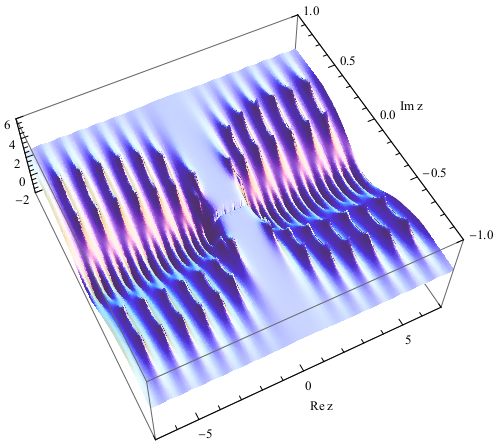
Refer to caption
Figure 12: Plot of the function −Re​(ln⁡(sinh⁡(B^​ρH​(z)))CLOSE-\text{Re}\left(\ln(\sinh(\hat{B}\rho_{\textsf{\tiny{H}}}(z))\right) in the complex zz-plane, for B=1B=1, μ=0.5\mu=0.5, T=0.3T=0.3 and 𝐮=0.1{\bf u}=0.1. The positive peaks correspond to energy-carrying Bethe roots, while the negative peaks on the real axis are zeros of sinh⁡(2​ϕ​(z))\sinh(2\phi(z)) (cf. equation (79)).

7.3 Exploring the complex plane

The numerical method we have described computes ρH​(z)\rho_{\textsf{\tiny{H}}}(z), ρV​(z)\rho_{\textsf{\tiny{V}}}(z) and Y1,1​(z)Y_{1,1}(z) for −1<z<1-1<z<1. Once we have a solution on the interval, we can reconstruct the behaviour of these functions in the complex plane. We do this in two steps. First, we use equation (133) to compute Y1,1​(z)Y_{1,1}(z) for zz on the whole first Riemann section – with cuts at z∈(−1,1)z\in(-1,1), z∈(−1,1)±2​i​𝐮z\in(-1,1)\pm 2i{\bf u} – from the values of the densities on the interval. From the same information, we can also compute 𝒢H​(z){\mathcal{G}}_{\textsf{\tiny{H}}}(z) and 𝒢V​(z){\mathcal{G}}_{\textsf{\tiny{V}}}(z) for an arbitrary complex value of zz. Then, one can obtain the values of ρH​(z)\rho_{\textsf{\tiny{H}}}(z), ρV​(z)\rho_{\textsf{\tiny{V}}}(z) for any complex values of zz by inverting (131). The complex zeros of sinh⁡(ρH​(z))\sinh(\rho_{\textsf{\tiny{H}}}(z)) are visible in Figure 12 for the numerical solution corresponding to μ=1/2\mu=1/2, B=1B=1, 𝐮=0.1{\bf u}=0.1, showing a clear qualitative similarity with the free fermion case.

8 Mirror equations

In this Section we shall describe the finite-size versions of the functional relations (84)-(86), which form a set of equations fully equivalent to the Lieb-Wu quantisation conditions (5),(6) with more general twisted boundary conditions. Comparing the thermal BA (14),(15) and the Lieb-Wu equations (5),(6), and considering the dispersion relations implied by (7), (77), one can see that the two systems are formally related by a simple map swapping L↔1/TL\leftrightarrow 1/T and single-particle energies with momenta1010 10 Notice that the identification of i​𝐤​(z)i{\bf k}(z) as the free energy carried by a Bethe root of rapidity zz is motivated by the discussion of Section 4.5. :

(𝐤⁡(z),𝜺⁡(z))⟶(−i​𝜺​(z),i​𝐤​(z)) L→1/T.\displaystyle\begin{array}[]{ccc}({\bf k}(z),\boldsymbol{\varepsilon}(z))&\longrightarrow&(-i\boldsymbol{\varepsilon}(z),i{\bf k}(z))\\ &\text{ $L\rightarrow 1/T$}&.\end{array}

Applying (8) to (84)-(86), we find a simple set of functional relations:

𝐩+H​(z)​𝐩~−H​(z)−𝐩~+H​(z)​𝐩−H​(z)\displaystyle{\bf p}_{{\boldsymbol{+}}}^{\textsf{\tiny{H}}}(z){\widetilde{\bf p}}^{\textsf{\tiny{H}}}_{{\boldsymbol{-}}}(z)-{\widetilde{\bf p}}^{\textsf{\tiny{H}}}_{{\boldsymbol{+}}}(z){\bf p}^{\textsf{\tiny{H}}}_{{\boldsymbol{-}}}(z) =\displaystyle= 2​i​sin⁡(L​𝐤​(z)),\displaystyle 2i\;\sin(L\,{\bf k}(z)), (142)
𝐩+V​(z)​𝐩~−V​(z)−𝐩~+V​(z)​𝐩−V​(z)\displaystyle{\bf p}^{\textsf{\tiny{V}}}_{{\boldsymbol{+}}}(z){\widetilde{\bf p}}^{\textsf{\tiny{V}}}_{{\boldsymbol{-}}}(z)-{\widetilde{\bf p}}^{\textsf{\tiny{V}}}_{{\boldsymbol{+}}}(z){\bf p}^{\textsf{\tiny{V}}}_{{\boldsymbol{-}}}(z) =\displaystyle= −2​i​sin⁡(L​𝐤​(z)),\displaystyle-2i\;\sin(L\,{\bf k}(z)), (143)
𝐩~aH​(z)​𝐩bV​(z)=𝐟a​b[+1]​(z)​e−i2​𝐤​(z)​L\displaystyle{\widetilde{\bf p}}_{a}^{\textsf{\tiny{H}}}(z){\bf p}^{\textsf{\tiny{V}}}_{b}(z)={\bf f}_{ab}^{[+1]}(z)e^{-\frac{i}{2}{\bf k}(z)\,L} +\displaystyle+ 𝐟a​b[−1](z)ei2​𝐤​(z)​L,a,b=+,−,\displaystyle{\bf f}_{ab}^{[-1]}(z)e^{\frac{i}{2}{\bf k}(z)\,L},\;\;\;a,b={\boldsymbol{+}},{\boldsymbol{-}}, (144)

where we require that the functions 𝐩aα​(z){\bf p}^{\alpha}_{a}(z) live on a two-sheeted Riemann surface, while the 𝐟a​b{\bf f}_{ab}’s are entire. Relations (142)-(144) can be seen as a set of Baxter-like equations for the Hubbard Hamiltonian. For LL an even integer, they admit many solutions where the 𝐟{\bf f}’s are polynomials; consequently, the 𝐩{\bf p}’s can be written as polynomial functions of 𝐱⁡(z){\bf x}(z) and 𝐱~​(z){\widetilde{\bf x}}(z), fixed in terms of their zeros on two sheets. For completeness, we can also consider exponential prefactors of the same type as the ones in (90), relabeling B→αB\rightarrow\alpha, μ→β\mu\rightarrow\beta. We then find easily the quantisation conditions for the following Bethe parameters: the zeros sjs_{j} of the 𝐩{\bf p}’s, and λl\lambda_{l} of the 𝐟{\bf f}’s. Setting 𝐤⁡(sj)=kj{\bf k}(s_{j})=k_{j}, and following the same route of Section 5, we find

ei​kj​L+i⁡(α^−β^)\displaystyle e^{ik_{j}L+i({\hat{\alpha}}-{\hat{\beta}})} =−∏l=1M(λl−sin⁡(kj)−i​𝐮λl−sin⁡(kj)+i​𝐮),j∈{1,…,N},\displaystyle=-\prod_{l=1}^{M}\left(\frac{\lambda_{l}-\sin(k_{j})-i{\bf u}}{\lambda_{l}-\sin(k_{j})+i{\bf u}}\right),\;\;j\in\left\{1,\dots,N\right\}, (145)
e−2​i​β^​∏j=1N(λl−sin⁡(kj)−i​𝐮λl−sin⁡(kj)+i​𝐮)\displaystyle e^{-2i{\hat{\beta}}}\,\prod_{j=1}^{N}\left(\frac{\lambda_{l}-\sin(k_{j})-i{\bf u}}{\lambda_{l}-\sin(k_{j})+i{\bf u}}\right) =∏m≠lm=1M(λl−λm−2​i​𝐮λl−λm+2​i​𝐮),l∈{1,…,M},\displaystyle=\prod_{{}^{m=1}_{m\neq l}}^{M}\left(\frac{\lambda_{l}-\lambda_{m}-2i{\bf u}}{\lambda_{l}-\lambda_{m}+2i{\bf u}}\right),\;\;l\in\left\{1,\dots,M\right\}, (146)

which is precisely the BA diagonalising the Hubbard Hamiltonian on the LL-site chain with twisted boundary conditions [58, 59]:

cL+1,↑=c1,↑​ei⁡(α^−β^−π),cL+1,↓=c1,↓​ei⁡(α^+β^−π).\displaystyle c_{L+1,\uparrow}=c_{1,\uparrow}\,e^{i({\hat{\alpha}}-{\hat{\beta}}-\pi)},\;\;\;\;c_{L+1,\downarrow}=c_{1,\downarrow}\,e^{i({\hat{\alpha}}+{\hat{\beta}}-\pi)}. (147)

The relation between the two Bethe Ansatz systems discussed above is directly connected to the path integral approach to the thermodynamics. Adopting the notation of [60], the latter is based on rewriting the partition function,

Z1D quantum=trVphyse−1/Tℋ,\displaystyle Z_{\text{1D quantum}}=\text{tr}_{V_{\text{phys}}}\,e^{-1/T\,\mathcal{H}}, (148)

of a spin chain of LL sites with Hamiltonian ℋ\mathcal{H}, as

Z1D quantum=limN¯→∞Z2D classical​(N¯,L,u)|u=1T​N¯,\displaystyle Z_{\text{1D quantum}}=\lim_{{\bar{N}}\rightarrow\infty}\left.Z_{\text{2D classical}}({\bar{N}},L,u)\right|_{u=\frac{1}{T{\bar{N}}}}, (149)

where Z2D classical​(N¯,L,u)Z_{\text{2D classical}}({\bar{N}},L,u) is the partition function of an appropriately defined two-dimensional statistical model living on a L×N¯L\times{\bar{N}} lattice. Its column-to-column transfer matrix is the Quantum Transfer Matrix TQTM​(u)T_{\text{QTM}}(u). By a π/2\pi/2 rotation on the lattice we switch from (148) to the description

Z1D quantum=limN¯→∞trVTrotter​(TQTM​(u))L|u=1T​N¯.\displaystyle Z_{\text{1D quantum}}=\lim_{{\bar{N}}\rightarrow\infty}\text{tr}_{V_{\text{Trotter}}}\left.(T_{\text{QTM}}(u))^{L}\right|_{u=\frac{1}{T{\bar{N}}}}. (150)

The exact Bethe Ansatz (14),(15) describes the spectrum of TQTMT_{\text{QTM}} in the Trotter limit N¯→∞{\bar{N}}\rightarrow\infty. It is an interesting open problem whether one can define the QTM directly in this limit, and give it a meaningful physical interpretation as a continuum model living on a space of size 1/T1/T.

A somehow similar problem has arisen in the context of AdS/CFT integrability, where Zamolodchikov’s ideas on the TBA for Lorentz invariant scattering theories [61] were adapted to the study of the non-relativistic string sigma model dual to planar 𝒩=4\mathcal{N}{=}4 SYM by considering its doubly Wick rotated counterpart (the mirror model) [31, 62]. Thanks to the knowledge of the action for the A​d​S5×S5AdS_{5}\times S^{5} string sigma model, it has recently been possible to identify the corresponding mirror model as a string theory living on a mirror background [63].

Finally, we would like to mention that is also possible to introduce a mirror version of Takahashi’s TBA, in such a way that it is equivalent to the finite-size BA (145),(146). Apart from minor subtleties 1111 11 For example, we think the −2𝐮/T-2{\bf u}/T term in (22) should be dropped., the mirror TBA equations can be obtained from (20)-(22) and the energy formula (27) through the following formal map :

𝜺⁡(z)\displaystyle\boldsymbol{\varepsilon}(z) →\displaystyle\rightarrow i​𝐤​(z),𝐤⁡(z)→−i​𝜺​(z),T→1/L,{B^,μ^}→{i​α^,i​β^},\displaystyle i{\bf k}(z),\;\;\;\;{\bf k}(z)\rightarrow-i\boldsymbol{\varepsilon}(z),\;\;\;T\rightarrow 1/L,\;\;\;\;\{\hat{B},\hat{\mu}\}\rightarrow\{i{\hat{\alpha}},i{\hat{\beta}}\}, (151)

and by modifying the integration contours as (cf [62, 28, 29, 30])

∫−1+i​0+1+i​0+→∫−∞+i​0+−1+i​0++∫1+i​0+∞+i​0+,\displaystyle\int_{-1+i0^{+}}^{1+i0^{+}}\rightarrow\int_{-\infty+i0^{+}}^{-1+i0^{+}}+\int_{1+i0^{+}}^{\infty+i0^{+}}, (152)

so that the roles of the mirror and magic sheets of Figures 4, 4 are interchanged1212 12 Due to this change in kinematics, the mirror TBA described here has some features in common with the TBA for the B model of [64], although the latter has a different dispersion relation. It would be interesting to investigate the relation between the two. . From these equations, one could in principle repeat the reduction presented in this paper and obtain the system (142)-(144).

9 Conclusions

The one-dimensional fermionic Hubbard model is one of the most interesting systems of low-dimensional condensed matter physics. Since its appearance in 1963, it has been intensively studied by means of exact and perturbative methods, greatly advancing the understanding of the physics of electron transport in 1D solids. A partial grasp about the huge number of results on this model can be obtained by consulting [65], the book [39] and the collections of works in [66, 67]. The purpose of this article is to add a little piece to the jigsaw, by recasting the Thermodynamic Bethe Ansatz equations of Takahashi as a nonlinear Riemann-Hilbert problem, reminiscent of the Quantum Spectral Curve formulation recently obtained for the study of anomalous dimensions in AdS/CFT [32]. One of the main results presented in this paper is a new set of nonlinear integral equations describing the thermodynamics of the system. In their region of validity (see discussion at the end of Section 7.2), these equations can be integrated numerically with very high precision and, even when implemented on Mathematica, the iterative algorithm converges in only a few seconds of CPU time. The complexity of this formulation is comparable to the system of nonlinear integral equations derived by Jüttner, Klümper and Suzuki in [16]. However, as a consequence of the fact that the equations proposed here are defined on a finite support, we think that they may prove more convenient for the study of finite temperature correlation lengths.

Acknowledgments – We are especially indebted to Nikolay Gromov and Junji Suzuki for many important suggestions and help. We also thank Davide Fioravanti, Fedor Levkovich-Maslyuk and Stefano Negro for many discussions and past collaboration on related topics, Stijn van Tongeren for useful correspondence and Volker Schomerus for encouragement and interest in the project. The research leading to these results has received funding from the People Programme (Marie Curie Actions) of the European Union’s Seventh Framework Programme FP7/2007-2013/ under REA Grant Agreement No 317089, from the INFN grant FTECP and the UniTo-SanPaolo research grant Nr TO-Call3-2012-0088 “Modern Applications of String Theory” (MAST).

Appendix A The magic sheet

In this Section we will show that the Y functions have the following cut structure on the magic sheet:

  • •

    Y1,n​(z)Y_{1,n}(z) and Yn,1​(z)Y_{n,1}(z) for n≥2n\geq 2 have only four branch cuts:

    z∈(−1,1)±i​𝐮​n,z∈(−1,1)±i​𝐮​(n+2),z\in(-1,1)\pm i{\bf u}n,\;\;\;\;z\in(-1,1)\pm i{\bf u}(n+2),
  • •

    Y1,1​(z)Y_{1,1}(z) and Y2,2​(z)Y_{2,2}(z) have only three branch cuts:

    z∈(−1,1),z∈(−1,1)±2​i​𝐮.z\in(-1,1),\;\;\;\;z\in(-1,1)\pm 2i{\bf u}.

As we will argue in Appendix B, a stronger property is true, namely the Y functions have no branch points outside the positions specified above, on any Riemann sheet. However, here we will present only the proof on the magic sheet, which is easier as it relies only on the structure of the Y-system and discontinuity relations. Before we start, we need to rewrite the Y-system (34) – originally defined on the mirror section – on the magic sheet. Using (31)-(33), it is simple to prove that the magic-sheet version of the Y-system is

Y1,n[+1]​Y1,n[−1]\displaystyle Y_{1,n}^{[+1]}\;Y_{1,n}^{[-1]} =\displaystyle= (1+Y1,n+1)​(1+Y1,n−1),n≥2\displaystyle(1+Y_{1,n+1})(1+Y_{1,n-1}),n\geq 2 (153)
1Yn,1[+1]​Yn,1[−1]\displaystyle\frac{1}{Y_{n,1}^{[+1]}\;Y_{n,1}^{[-1]}} =\displaystyle= (1+1/Yn+1,1)​(1+1/Yn−1,1),n≥2,\displaystyle(1+1/Y_{n+1,1})(1+1/Y_{n-1,1}),\;\;\;n\geq 2, (154)
Y1,1[+1]Y2,2[−1]\displaystyle\frac{Y_{1,1}^{[+1]}}{Y_{2,2}^{[-1]}} =\displaystyle= (1+Y1,21+1/Y2,1).\displaystyle\left(\frac{1+Y_{1,2}}{1+1/Y_{2,1}}\right). (155)

We will now test the cut structure of the Y1,n+1Y_{1,n+1} functions for n≥1n\geq 1. First, let us introduce

Xn=(1+Y1,n[n+1]Y1,n[n+1])​(1+Y1,n+1[n]Y1,n+1[n]),n≥2.\displaystyle X_{n}=\left(\frac{1+Y_{1,n}^{[n+1]}}{Y_{1,n}^{[n+1]}}\right)\left(\frac{1+Y_{1,n+1}^{[n]}}{Y_{1,n+1}^{[n]}}\right),\;\;\;\;\;n\geq 2. (156)

These combinations are useful since, applying (153) in two elementary steps, it is possible to prove that

Y1,n[n+3](1+Y1,n−1[n+2])1−δn,2=Xn​Xn+1​(1+Y1,n+3[n]Y1,n+2[n−1]),n≥2.\displaystyle\frac{Y_{1,n}^{[n+3]}}{(1+Y_{1,n-1}^{[n+2]})^{1-\delta_{n,2}}}=X_{n}\;X_{n+1}\left(\frac{1+Y_{1,n+3}^{[n]}}{Y_{1,n+2}^{[n-1]}}\right),\;\;\;\;n\geq 2. (157)

Notice that the term in brackets in (157) has no cut because it falls into the analyticity strip. Therefore, the cut structure of the lhs of (157) depends on the XnX_{n} factors. We shall now show that XnX_{n} have no cut on the real axis, for all n≥2n\geq 2. Starting from n=2n=2, we can compute

X2=(1+Y1,2[3])​(1+Y1,3[2])Y1,2[3]​Y1,3[2]=Y1,2[1]​(1+Y1,2[3])Y1,3[2]=(Y1,2[1]+1+Y1,3[2])Y1,3[2]=1+Y1,3(1+Y1,4[1]).\displaystyle X_{2}=\frac{(1+Y_{1,2}^{[3]})(1+Y_{1,3}^{[2]})}{Y_{1,2}^{[3]}Y_{1,3}^{[2]}}=\frac{Y_{1,2}^{[1]}(1+Y_{1,2}^{[3]})}{Y_{1,3}^{[2]}}=\frac{(Y_{1,2}^{[1]}+1+Y_{1,3}^{[2]})}{Y_{1,3}^{[2]}}=1+\frac{Y_{1,3}}{(1+Y_{1,4}^{[1]})}. (158)

This expression manifestly does not have branch points on the real axis, as all terms on the rhs fall into their respective analyticity strips. A very similar calculation shows that

X3\displaystyle X_{3} =\displaystyle= (1+Y1,3[4])​(1+Y1,4[3])Y1,3[4]​Y1,4[3]=Y1,3[2]​(1+Y1,3[4])Y1,4[3]​(1+Y1,2[3])=Y1,3[2]+(1+Y1,4[3])​(1+Y1,2[3])Y1,4[3]​(1+Y1,2[3])\displaystyle\frac{(1+Y_{1,3}^{[4]})(1+Y_{1,4}^{[3]})}{Y_{1,3}^{[4]}Y_{1,4}^{[3]}}=\frac{Y_{1,3}^{[2]}(1+Y_{1,3}^{[4]})}{Y_{1,4}^{[3]}(1+Y_{1,2}^{[3]})}=\frac{Y_{1,3}^{[2]}+(1+Y_{1,4}^{[3]})(1+Y_{1,2}^{[3]})}{Y_{1,4}^{[3]}(1+Y_{1,2}^{[3]})} (159)
=\displaystyle= 1+Y1,4[1]​(Y1,3[2]+1+Y1,2[3])(1+Y1,5[2])​(1+Y1,3[2])​(1+Y1,2[3])=1+Y1,4[1](1+Y1,5[2])−1X2​Y1,4[1](1+Y1,5[2]),\displaystyle 1+\frac{Y_{1,4}^{[1]}(Y_{1,3}^{[2]}+1+Y_{1,2}^{[3]})}{(1+Y_{1,5}^{[2]})(1+Y_{1,3}^{[2]})(1+Y_{1,2}^{[3]})}=1+\frac{Y_{1,4}^{[1]}}{(1+Y_{1,5}^{[2]})}-\frac{1}{X_{2}}\;\frac{Y_{1,4}^{[1]}}{(1+Y_{1,5}^{[2]})},

and, literally by repeating this calculation with shifted indices, one finds the general case:

Xn+1=1+(Y1,n+1[n−2]1+Y1,n+2[n−1])−1Xn​(Y1,n+2[n−1]1+Y1,n+3[n]),n≥2.\displaystyle X_{n+1}=1+\left(\frac{Y_{1,n+1}^{[n-2]}}{1+Y_{1,n+2}^{[n-1]}}\right)-\frac{1}{X_{n}}\left(\frac{Y_{1,n+2}^{[n-1]}}{1+Y_{1,n+3}^{[n]}}\right),\;\;\;\;\;n\geq 2. (160)

Taking into account the analyticity strips of the functions on the rhs, this equation shows by induction that all XnX_{n} are free of cuts. Therefore, the lhs of (157) is analytic in a neighbourhood of the real axis, meaning that Y1,nY_{1,n} with n≥2n\geq 2 has possibly two cuts in the upper half plane at Im​(z)=𝐮​(n±1)\text{Im}(z)={\bf u}(n\pm 1), but no cut at Im​(z)=𝐮​(n+3)\text{Im}(z)={\bf u}(n+3). Moreover, because of the Y-system, no further cuts are possible and the Y1,nY_{1,n}’s with n≥2n\geq 2 have only two short branch cuts in the upper half plane. By symmetry, the argument can be repeated for the lower half plane and for the Yn,1Y_{n,1} functions with n≥2n\geq 2.
The argument presented above (contrary to the remaining part of this Appendix) can be straightforwardly adapted to the horizontal wing of the AdS/CFT Y-systems.

Let us now prove that Y1,1Y_{1,1} and Y2,2Y_{2,2} have only three cuts. Using (153), we can compute

Y1,1[4]\displaystyle Y_{1,1}^{[4]} =\displaystyle= Y2,2[2]​(1+Y1,2[3]1+1/Y2,1[3])=Y2,2[2]​(1+(1+Y1,3[2])/Y1,2[1]1+(1+1/Y3,1[2])​Y2,1[1])\displaystyle Y_{2,2}^{[2]}\;\left(\frac{1+Y_{1,2}^{[3]}}{1+1/Y_{2,1}^{[3]}}\right)=Y_{2,2}^{[2]}\;\left(\frac{1+(1+Y_{1,3}^{[2]})/Y_{1,2}^{[1]}}{1+(1+1/Y_{3,1}^{[2]})Y_{2,1}^{[1]}}\right) (161)
=\displaystyle= Y2,2[2]Y1,2[1]​Y2,1[1]​(1+Y1,2[1]1+1/Y2,1[1])​R=Y1,1[2]​Y2,2[2]Y1,2[1]​Y2,1[1]​Y2,2​R,\displaystyle\frac{Y_{2,2}^{[2]}}{Y_{1,2}^{[1]}Y_{2,1}^{[1]}}\;\left(\frac{1+Y_{1,2}^{[1]}}{1+1/Y_{2,1}^{[1]}}\right)\,R=\frac{Y_{1,1}^{[2]}Y_{2,2}^{[2]}}{Y_{1,2}^{[1]}Y_{2,1}^{[1]}Y_{2,2}}\;R, (162)

where RR manifestly has no cut on the real axis and is defined by

R=(1+Y1,3[2]/(1+Y1,2[1])1+(Y3,1[2])−1/(1+1/Y2,1[1]))=(1+(1+Y1,4[1])/Y1,31+(1+1/Y4,1[1])​Y3,1).\displaystyle R=\left(\frac{1+Y_{1,3}^{[2]}/(1+Y_{1,2}^{[1]})}{1+(Y_{3,1}^{[2]})^{-1}/(1+1/Y_{2,1}^{[1]})}\right)=\left(\frac{1+(1+Y_{1,4}^{[1]})/Y_{1,3}}{1+(1+1/Y_{4,1}^{[1]})Y_{3,1}}\right). (163)

Because Y1,1​(z)​Y2,2​(z)=e−4​ϕ​(z)Y_{1,1}(z)Y_{2,2}(z)=e^{-4\,\phi(z)} has no cuts outside the real axis, the only discontinuity can come from the factor:

H=1/(Y1,2[1]​Y2,1[1]​Y2,2).\displaystyle H=1/(Y_{1,2}^{[1]}Y_{2,1}^{[1]}Y_{2,2}). (164)

Using the discontinuity relations (31)-(33), we find

H~H=1+1/Y1,11+Y2,2​1+1/Y2,21+Y1,1​Y2,2Y~2,2=1.\displaystyle\frac{{\widetilde{H}}}{H}=\frac{1+1/Y_{1,1}}{1+Y_{2,2}}\;\frac{1+1/Y_{2,2}}{1+Y_{1,1}}\;\frac{Y_{2,2}}{{\widetilde{Y}}_{2,2}}=1. (165)

This shows that Y1,1Y_{1,1} (and therefore also Y2,2Y_{2,2}) does not have a branch cut with Im​(z)=4​𝐮\text{Im}(z)=4{\bf u}. The Y-system, together with the results already obtained for the other Y functions, imply that no further cuts are possible.

Appendix B Monodromy properties of the 𝐏{\bf P} functions

The purpose of this Appendix is to provide a proof for some statements made in Section 4.

  1. 1)

    First, we prove that it is possible to choose the 𝕋\mathbb{T} gauges in such a way that equation (44) holds, namely

    𝕋1,0H​(z)=e−2​ϕ​(z),𝕋0,1V​(z)=e2​ϕ​(z).\displaystyle\mathbb{T}_{1,0}^{\textsf{\tiny{H}}}(z)=e^{-2\phi(z)},\;\;\;\;\;\mathbb{T}_{0,1}^{\textsf{\tiny{V}}}(z)=e^{2\phi(z)}. (166)

    In the proof we will use the resolvent parametrisation of Section 4.3, which, rigorously speaking, is valid only for the ground state. However, we expect that the result holds in general.

  2. 2)

    Secondly, we derive the constraints (51), (52).

  3. 3)

    Finally, we discuss how to infer that the second-sheet evaluation of the 𝐏{\bf P} functions, 𝐏~{\widetilde{\bf P}}, do not have other branch cuts apart from z∈(−1,1)z\in(-1,1). This shows that the 𝐏{\bf P}’s live on a Riemann surface with only two sheets.

To prove these properties, we will adapt many of the arguments of [44] to the present case.

Proof of equation (44) for 𝕋1,0H\mathbb{T}_{1,0}^{\textsf{\tiny{H}}} and 𝕋0,1V\mathbb{T}_{0,1}^{\textsf{\tiny{V}}}

To verify the statement 1), let us start from the gauge 𝒯H{{\mathcal{T}}}^{\textsf{\tiny{H}}} (we restrict to the horizontal wing since the situation is clearly analogous for the vertical wing). This gauge is defined by the parametrisation

𝒯1,nH\displaystyle{{\mathcal{T}}}^{\textsf{\tiny{H}}}_{1,n} =\displaystyle= sinh⁡(B^​(1+𝒢H[+n]−𝒢H[−n]))/sinh⁡(B^),n≥1,\displaystyle\sinh\left(\hat{B}(1+{\mathcal{G}}^{[+n]}_{\textsf{\tiny{H}}}-{\mathcal{G}}^{[-n]}_{\textsf{\tiny{H}}})\right)/\sinh(\hat{B}),\;\;n\geq 1,
𝒯0,sH\displaystyle{{{\mathcal{T}}}}^{\textsf{\tiny{H}}}_{0,s} =\displaystyle= 1,s∈ℕ,𝒯2,lH=𝒯1,1H​[+l]​𝒯1,1H​[−l],l≥2.\displaystyle 1,\;\;s\in\mathbb{N},\;\;\;\;\;\;\;\;{{{\mathcal{T}}}}^{\textsf{\tiny{H}}}_{2,l}={{{\mathcal{T}}}}^{\textsf{\tiny{H}}\,[+l]}_{1,1}\;{{{\mathcal{T}}}}^{\textsf{\tiny{H}}\,[-l]}_{1,1},\;\;l\geq 2. (167)

with the resolvent density ρH\rho_{\textsf{\tiny{H}}} fixed uniquely, in terms of the Y functions, through equation (131). We shall prove that1313 13 The analogous expression for the upper wing is 𝒯0,1V​(z)=sinh⁡(μ^​ρV​(z))2​sinh⁡(2​ϕ​(z))​sinh⁡(μ^)​e2​ϕ​(z).\displaystyle{{\mathcal{T}}}_{0,1}^{\textsf{\tiny{V}}}(z)=\frac{\sinh(\hat{\mu}\rho_{\textsf{\tiny{V}}}(z))}{2\sinh(2\phi(z))\sinh(\hat{\mu})}\;e^{2\phi(z)}.

𝒯1,0H​(z)=sinh⁡(B^​ρH​(z))2​sinh⁡(2​ϕ​(z))​sinh⁡(B^)​e−2​ϕ​(z).\displaystyle{{\mathcal{T}}}_{1,0}^{\textsf{\tiny{H}}}(z)=\frac{\sinh(\hat{B}\rho_{\textsf{\tiny{H}}}(z))}{2\sinh(2\phi(z))\sinh(\hat{B})}\;e^{-2\phi(z)}. (168)

We start by rewriting some of the discontinuity relations (31)-(34) in terms of the 𝒯H{{\mathcal{T}}}^{\textsf{\tiny{H}}} functions. Using the properties of this gauge, equation Y1,1=1/Y~2,2Y_{1,1}=1/\widetilde{Y}_{2,2} can be written as

𝒯~1,0H=𝒯3,2H/𝒯2,3H​(𝒯~2,1H𝒯2,1H),\displaystyle{\widetilde{{{\mathcal{T}}}}_{1,0}^{\textsf{\tiny{H}}}}={{\mathcal{T}}}_{3,2}^{\textsf{\tiny{H}}}/{{\mathcal{T}}}_{2,3}^{\textsf{\tiny{H}}}\,\left(\frac{{\widetilde{{\mathcal{T}}}}_{2,1}^{\textsf{\tiny{H}}}}{{{\mathcal{T}}}_{2,1}^{\textsf{\tiny{H}}}}\right), (169)

while the relation Y1,1​Y2,2=e−4​ϕY_{1,1}\,Y_{2,2}=e^{-4\phi} becomes

e−4​ϕ=𝒯1,0H​𝒯2,3H𝒯3,2H=𝒯1,0H𝒯1,0H~​(𝒯~2,1H𝒯2,1H).\displaystyle e^{-4\phi}=\frac{{{\mathcal{T}}}_{1,0}^{\textsf{\tiny{H}}}{{\mathcal{T}}}_{2,3}^{\textsf{\tiny{H}}}}{{{\mathcal{T}}}_{3,2}^{\textsf{\tiny{H}}}}=\frac{{{\mathcal{T}}}_{1,0}^{\textsf{\tiny{H}}}}{{\widetilde{{{\mathcal{T}}}_{1,0}^{\textsf{\tiny{H}}}}}}\,\left(\frac{{\widetilde{{\mathcal{T}}}}_{2,1}^{\textsf{\tiny{H}}}}{{{\mathcal{T}}}_{2,1}^{\textsf{\tiny{H}}}}\right). (170)

The equation involving Y1,2Y_{1,2} is automatically satisfied by the parametrisation (167), while the equation for Y2,1Y_{2,1} will be used later. Now, we compare the T-system equations at the nodes (1,1)(1,1) and (2,2)(2,2). On the magic sheet, these two equations read

𝒯1,1H​[+1]~​𝒯1,1H​[−1]\displaystyle{\widetilde{{{\mathcal{T}}}_{1,1}^{\textsf{\tiny{H}}\,[+1]}}}\,{{\mathcal{T}}}_{1,1}^{\textsf{\tiny{H}}\,[-1]} =\displaystyle= 𝒯1,0H​𝒯1,2H+𝒯2,1H,\displaystyle{{\mathcal{T}}}_{1,0}^{\textsf{\tiny{H}}}{{\mathcal{T}}}_{1,2}^{\textsf{\tiny{H}}}+{{\mathcal{T}}}_{2,1}^{\textsf{\tiny{H}}}, (171)
𝒯2,2H​[+1]~​𝒯2,2H​[−1]\displaystyle{\widetilde{{{\mathcal{T}}}_{2,2}^{\textsf{\tiny{H}}\,[+1]}}}\,{{\mathcal{T}}}_{2,2}^{\textsf{\tiny{H}}\,[-1]} =\displaystyle= 𝒯1,1H​[+1]​𝒯1,1H​[−1]~​𝒯2,3H=𝒯2,3H​𝒯2,1H+𝒯3,2H​𝒯1,2H.\displaystyle{{\mathcal{T}}}_{1,1}^{\textsf{\tiny{H}}\,[+1]}\,{\widetilde{{{\mathcal{T}}}_{1,1}^{\textsf{\tiny{H}}\,[-1]}}}\,{{\mathcal{T}}}_{2,3}^{\textsf{\tiny{H}}}={{\mathcal{T}}}_{2,3}^{\textsf{\tiny{H}}}{{\mathcal{T}}}_{2,1}^{\textsf{\tiny{H}}}+{{\mathcal{T}}}_{3,2}^{\textsf{\tiny{H}}}{{\mathcal{T}}}_{1,2}^{\textsf{\tiny{H}}}. (172)

The identity (172) was derived using 𝒯2,sH=𝒯1,1H​[+s]​𝒯1,1H​[−s]{{\mathcal{T}}}_{2,s}^{\textsf{\tiny{H}}}={{\mathcal{T}}}_{1,1}^{\textsf{\tiny{H}}\,[+s]}\,{{\mathcal{T}}}_{1,1}^{\textsf{\tiny{H}}\,[-s]}. Eliminating 𝒯21H{{\mathcal{T}}}_{21}^{\textsf{\tiny{H}}} from these equations shows that

disc​[𝒯1,1H​[+1]~​𝒯1,1H​[−1]]=𝒯1,2H​(𝒯1,0H−𝒯3,2/𝒯2,3H)=𝒯1,2H​𝒯1,0H​(1−e4​ϕ),\displaystyle\text{disc}\left[{\widetilde{{{\mathcal{T}}}_{1,1}^{\textsf{\tiny{H}}\,[+1]}}}\,{{\mathcal{T}}}_{1,1}^{\textsf{\tiny{H}}\,[-1]}\right]={{\mathcal{T}}}_{1,2}^{\textsf{\tiny{H}}}\left({{\mathcal{T}}}_{1,0}^{\textsf{\tiny{H}}}-{{\mathcal{T}}}_{3,2}/{{\mathcal{T}}}_{2,3}^{\textsf{\tiny{H}}}\right)={{\mathcal{T}}}_{1,2}^{\textsf{\tiny{H}}}\,{{\mathcal{T}}}_{1,0}^{\textsf{\tiny{H}}}\left(1-e^{4\phi}\right), (173)

where we have used (170) in the last step. Using (167) in (173), we find the result quoted in (168). To construct the gauge 𝕋H\mathbb{T}^{\textsf{\tiny{H}}}, we can now introduce the gauge transformation factor 𝐡H{\bf h}_{\textsf{\tiny{H}}} through equation (62), so that 𝐡H​𝐡~H=sinh⁡(2​ϕ​sinh⁡(B^))/sinh⁡(B^​ρH){\bf h}_{\textsf{\tiny{H}}}{\widetilde{\bf h}}_{\textsf{\tiny{H}}}=\sinh(2\phi\sinh(\hat{B}))/\sinh(\hat{B}\rho_{\textsf{\tiny{H}}}). Defining the 𝕋H\mathbb{T}^{\textsf{\tiny{H}}} gauge through

𝕋1,sH=𝐡H[s]​𝐡H[−s]​𝒯1,sH,s∈ℕ+,𝕋0,nH=1,n∈ℕ,\displaystyle\mathbb{T}^{\textsf{\tiny{H}}}_{1,s}={\bf h}_{\textsf{\tiny{H}}}^{[s]}{\bf h}_{\textsf{\tiny{H}}}^{[-s]}\,{{\mathcal{T}}}_{1,s}^{\textsf{\tiny{H}}},\;\;\;s\in\mathbb{N}^{+},\;\;\;\;\mathbb{T}_{0,n}^{\textsf{\tiny{H}}}=1,\;\;\;n\in\mathbb{N}, (174)

we finally arrive at

𝕋1,0H​(z)=𝐡H​(z)​𝐡~H​(z)​𝒯1,0H​(z)=e−2​ϕ​(z).\displaystyle\mathbb{T}_{1,0}^{\textsf{\tiny{H}}}(z)={\bf h}_{\textsf{\tiny{H}}}(z){\widetilde{\bf h}}_{\textsf{\tiny{H}}}(z)\,{{\mathcal{T}}}_{1,0}^{\textsf{\tiny{H}}}(z)=e^{-2\phi(z)}. (175)

Proof of the constraints (51),(52)

Statement 2) can be proved by revisiting the derivation of (173) given above in the case of the gauge 𝕋H\mathbb{T}^{\textsf{\tiny{H}}}. This leads to

disc​[𝕋1,1H​[+1]~​𝕋1,1H​[−1]]=𝕋1,2H​𝕋1,0H​(1−e4​ϕ).\displaystyle\text{disc}\left[{\widetilde{\mathbb{T}_{1,1}^{\textsf{\tiny{H}}\,[+1]}}}\,\mathbb{T}_{1,1}^{\textsf{\tiny{H}}\,[-1]}\right]=\mathbb{T}_{1,2}^{\textsf{\tiny{H}}}\,\mathbb{T}_{1,0}^{\textsf{\tiny{H}}}\left(1-e^{4\phi}\right). (176)

The constraint (51) follows from (176) using (166) and the expression of the 𝕋H\mathbb{T}^{\textsf{\tiny{H}}} functions in terms of 𝐏H{\bf P}^{\textsf{\tiny{H}}}’s. One can also derive an equation analogous to (176) with H→V\textsf{H}\rightarrow\textsf{V}, ϕ→−ϕ\phi\rightarrow-\phi, and prove (52) by the same method.

Proof that the 𝐏{\bf P} functions have only a single cut on the second sheet

Statement 3): let us now sketch the proof that the 𝐏{\bf P}’s have no cut outside the real axis even on their second Riemann sheet, and, therefore, live on a two-sheeted surface. The proof is very similar to the ones used in a more complicated context in [33, 37]. To start, we observe that, due to (168), the ratio in brackets in (169) and (170) is actually one, so that 𝒯~2,1H=𝒯2,1H{\widetilde{{\mathcal{T}}}}_{2,1}^{\textsf{\tiny{H}}}={{\mathcal{T}}}^{\textsf{\tiny{H}}}_{2,1}. Since 𝕋2,1H=𝐡H[+2]​𝐡H[−2]​𝐡H​𝐡~H​𝒯2,1H\mathbb{T}_{2,1}^{\textsf{\tiny{H}}}={\bf h}_{\textsf{\tiny{H}}}^{[+2]}\;{\bf h}_{\textsf{\tiny{H}}}^{[-2]}\;{\bf h}_{\textsf{\tiny{H}}}\;{\widetilde{{\bf h}}_{\textsf{\tiny{H}}}}\,{{\mathcal{T}}}_{2,1}^{\textsf{\tiny{H}}}, we find that also 𝕋2,1H\mathbb{T}^{\textsf{\tiny{H}}}_{2,1} has no cut on the real axis:

𝕋2,1H=𝕋~2,1H.\displaystyle\mathbb{T}_{2,1}^{\textsf{\tiny{H}}}={\widetilde{\mathbb{T}}}_{2,1}^{\textsf{\tiny{H}}}. (177)

Furthermore, notice that we have not used yet the discontinuity equation (33) involving Y2,1Y_{2,1}. Rewriting this relation in terms of T functions in the gauge 𝕋H\mathbb{T}^{\textsf{\tiny{H}}}, we find

𝕋1,1H​[+1]​𝕋1,1H​[−1]𝕋2,2H​[+1]​𝕋2,2H​[−1]=𝕋1,0H𝕋3,2H​𝕋3,1H​[+1]~​𝕋2,0H​[+1]𝕋3,1H​[+1]​𝕋2,0H​[+1]~.\displaystyle\frac{{\mathbb{T}_{1,1}^{\textsf{\tiny{H}}\,[+1]}}\,\mathbb{T}_{1,1}^{\textsf{\tiny{H}}\,[-1]}}{\mathbb{T}_{2,2}^{\textsf{\tiny{H}}\,[+1]}\,\mathbb{T}_{2,2}^{\textsf{\tiny{H}}\,[-1]}}=\frac{\mathbb{T}_{1,0}^{\textsf{\tiny{H}}}}{\mathbb{T}_{3,2}^{\textsf{\tiny{H}}}}\,\frac{\widetilde{\mathbb{T}_{3,1}^{\textsf{\tiny{H}}\,[+1]}}\,{\mathbb{T}_{2,0}^{\textsf{\tiny{H}}\,[+1]}}}{\mathbb{T}_{3,1}^{\textsf{\tiny{H}}\,[+1]}\,\widetilde{\mathbb{T}_{2,0}^{\textsf{\tiny{H}}\,[+1]}}}. (178)

The ratio on the lhs side can be simplified using 𝕋2,2H=𝕋1,1H​[+2]​𝕋1,1H​[−2]\mathbb{T}_{2,2}^{\textsf{\tiny{H}}}=\mathbb{T}_{1,1}^{\textsf{\tiny{H}}[+2]}\mathbb{T}_{1,1}^{\textsf{\tiny{H}}[-2]}, and leads to

1=𝕋1,0H​𝕋2,3H𝕋3,2H​𝕋3,1H​[+1]~​𝕋2,0H​[+1]𝕋3,1H​[+1]​𝕋2,0H​[+1]~=e−4​ϕ​𝕋3,1H​[+1]~​𝕋2,0H​[+1]𝕋3,1H​[+1]​𝕋2,0H​[+1]~.\displaystyle 1=\frac{\mathbb{T}_{1,0}^{\textsf{\tiny{H}}}\,\mathbb{T}_{2,3}^{\textsf{\tiny{H}}}}{\mathbb{T}_{3,2}^{\textsf{\tiny{H}}}}\,\frac{\widetilde{\mathbb{T}_{3,1}^{\textsf{\tiny{H}}\,[+1]}}\,{\mathbb{T}_{2,0}^{\textsf{\tiny{H}}\,[+1]}}}{\mathbb{T}_{3,1}^{\textsf{\tiny{H}}\,[+1]}\,\widetilde{\mathbb{T}_{2,0}^{\textsf{\tiny{H}}\,[+1]}}}=e^{-4\phi}\,\,\frac{\widetilde{\mathbb{T}_{3,1}^{\textsf{\tiny{H}}\,[+1]}}\,{\mathbb{T}_{2,0}^{\textsf{\tiny{H}}\,[+1]}}}{\mathbb{T}_{3,1}^{\textsf{\tiny{H}}\,[+1]}\,\widetilde{\mathbb{T}_{2,0}^{\textsf{\tiny{H}}\,[+1]}}}. (179)

Using the T-system and (166), it is simple to compute the factor involving 𝕋2,0H\mathbb{T}_{2,0}^{\textsf{\tiny{H}}}, and finally (179) reduces to the condition

𝕋3,1H​[+1]=𝕋3,1H​[+1]~.\displaystyle\mathbb{T}_{3,1}^{\textsf{\tiny{H}}\,[+1]}=\widetilde{\mathbb{T}_{3,1}^{\textsf{\tiny{H}}\,[+1]}}. (180)

Furthermore, using the discontinuity relations

Yn+1,1[n]/Yn+1,1[n]~=(1+1/Yn,1[n−1])/(1+1/Yn,1[n−1]~),n∈ℕ+,\displaystyle Y_{n+1,1}^{[n]}/\widetilde{Y_{n+1,1}^{[n]}}=\left(1+1/Y_{n,1}^{[n-1]}\right)/\left(1+1/\widetilde{Y_{n,1}^{[n-1]}}\right),\;\;\;n\in\mathbb{N}^{+}, (181)

which follow from the Y-system, it is possible to generalise (177) and (180) to

disc[𝕋n,1H​[n−2]]=0,n=2,3,….\displaystyle\text{disc}\left[\mathbb{T}_{n,1}^{\textsf{\tiny{H}}\,[n-2]}\right]=0,\;\;\;n=2,3,\dots. (182)

The set of equations (182) can be used to prove that the 𝐏{\bf P}’s live on a two-sheeted Riemann surface. By definition, these functions have a single cut on their first sheet, and parametrise some of the 𝕋H\mathbb{T}^{\textsf{\tiny{H}}}’s as

𝕋1,sH=𝐏+H​[+s]​𝐏−H​[−s]−𝐏+H​[−s]​𝐏−H​[+s],s∈ℕ+.\displaystyle\mathbb{T}_{1,s}^{\textsf{\tiny{H}}}={\bf P}_{{\boldsymbol{+}}}^{\textsf{\tiny{H}}\,[+s]}{\bf P}_{{\boldsymbol{-}}}^{\textsf{\tiny{H}}\,[-s]}-{\bf P}_{{\boldsymbol{+}}}^{\textsf{\tiny{H}}\,[-s]}{\bf P}_{{\boldsymbol{-}}}^{\textsf{\tiny{H}}\,[+s]},\;\;\;s\in\mathbb{N}^{+}. (183)

Hirota equation (39) allows to extend (183) and compute any 𝕋H\mathbb{T}^{\textsf{\tiny{H}}} function in terms of the 𝐏H{\bf P}^{\textsf{\tiny{H}}}’s. However, since (39) is defined on the mirror section, the computation may require to explore the values of the 𝐏{\bf P} functions on the second sheet. In particular, it can be easily checked that 𝕋n,1H,[n−2]\mathbb{T}^{\textsf{\tiny{H}},[n-2]}_{n,1} with n>1n>1 involves (linearly) the values of 𝐏~±H,[2​n−2]{\widetilde{\bf P}}^{\textsf{\tiny{H}},[2n-2]}_{{\boldsymbol{\pm}}}, so that imposing the constraints (182) gives information on the possible cuts of the 𝐏~H{\widetilde{\bf P}}^{\textsf{\tiny{H}}}’s. For instance, from equation (177), one can recover the constraint (51). With the aid of this result, the other equations in (182) can be used to prove that

𝐏~±H​[+n]−𝐏~±H​[+n]~=0,n∈ℕ+.\displaystyle{\widetilde{{\bf P}}}_{{\boldsymbol{\pm}}}^{\textsf{\tiny{H}}\,[+n]}-{\widetilde{{\widetilde{{\bf P}}}_{{\boldsymbol{\pm}}}^{\textsf{\tiny{H}}\,[+n]}}}=0,\;\;n\in\mathbb{N}^{+}. (184)

Obviously, by symmetry all these results are valid both in the upper and in the lower half complex plane, and show that 𝐏~±H{\widetilde{\bf P}}^{\textsf{\tiny{H}}}_{{\boldsymbol{\pm}}} have no cuts outside the real axis.

Appendix C Fixing the gauge factor 𝕋H/𝕋V\mathbb{T}^{\textsf{\tiny{H}}}/\mathbb{T}^{\textsf{\tiny{V}}}

The main purpose of this Appendix is to derive the form of the gauge transformation (45)-(47) relating the 𝕋H\mathbb{T}^{\textsf{\tiny{H}}} and 𝕋V\mathbb{T}^{\textsf{\tiny{V}}} functions. Along the way, we will also obtain the two NLIEs (188) and (192), adopted for the numerical solution method described in Section 7.
Let us briefly discuss the logic of this Section. In Appendix B, we have encoded the discontinuity equations (31)-(34) in the simple statement that the 𝐏{\bf P} functions live on a two-sheeted Riemann surface and satisfy the relations (51),(52). However, some information is still missing to close the system. In fact, notice that, when describing the system with the functions 𝐏±H{\bf P}^{\textsf{\tiny{H}}}_{{\boldsymbol{\pm}}}, there is nothing to guarantee the correct large zz behaviour (35) for the Yn,1Y_{n,1}’s with n≥1n\geq 1. To fill this gap we will extract an extra equation from the TBA, equation (190), and show that it fixes the form of the gauge transformation (45)-(47). Finally, we will show that the final set of equations (51)-(53) is self-consistent and that equation (190) can be rederived from them.

Direct proof

The Y function sitting at the central node can be parametrised equivalently using the gauges 𝒯H{{\mathcal{T}}}^{\textsf{\tiny{H}}} or 𝒯V{{\mathcal{T}}}^{\textsf{\tiny{V}}}. This gives the two expressions

1+1/Y1,1\displaystyle 1+1/Y_{1,1} =\displaystyle= 2​e2​ϕ​sinh⁡(2​ϕ)​sinh⁡(B^)sinh⁡(B^​ρH)​𝒯1,1H​[+1]~​𝒯1,1H​[−1]𝒯1,2H,\displaystyle 2\frac{e^{2\phi}\sinh(2\phi)\sinh(\hat{B})}{\sinh(\hat{B}\rho_{\textsf{\tiny{H}}})}\;\frac{{\widetilde{{{\mathcal{T}}}^{\textsf{\tiny{H}}\,[+1]}_{1,1}}}\;{{\mathcal{T}}}^{\textsf{\tiny{H}}\,[-1]}_{1,1}}{{{\mathcal{T}}}^{\textsf{\tiny{H}}}_{1,2}}, (185)
1+Y1,1\displaystyle 1+Y_{1,1} =\displaystyle= −2​e−2​ϕ​sinh⁡(2​ϕ)​sinh⁡(μ^)sinh⁡(μ^​ρV)​𝒯1,1V​[+1]~​𝒯1,1V​[−1]𝒯2,1V.\displaystyle-2\frac{e^{-2\phi}\sinh(2\phi)\sinh(\hat{\mu})}{\sinh(\hat{\mu}\rho_{\textsf{\tiny{V}}})}\;\frac{{\widetilde{{{\mathcal{T}}}^{\textsf{\tiny{V}}\,[+1]}_{1,1}}}\;{{\mathcal{T}}}^{\textsf{\tiny{V}}\,[-1]}_{1,1}}{{{\mathcal{T}}}^{\textsf{\tiny{V}}}_{2,1}}. (186)

Constructing the quantity

r⁡(z)=(1+1/Y2,2​(z)1+Y1,1​(z))=(1+Y1,1​(z)​e4​ϕ​(z)1+Y1,1​(z)),\displaystyle r(z)=\left(\frac{1+1/Y_{2,2}(z)}{1+Y_{1,1}(z)}\right)=\left(\frac{1+Y_{1,1}(z)\;e^{4\phi(z)}}{1+Y_{1,1}(z)}\right), (187)

and matching the alternative expressions for r⁡(z)r(z) obtained from (185) and (186) gives the first equation of the NLIEs written in Section 7:

r⁡(z)=𝒯1,1H​[+1]​(z)​𝒯1,1H​[−1]~​(z)𝒯1,1H​[−1]​(z)​𝒯1,1H​[+1]~​(z)=e4​ϕ​(z)​𝒯1,1V​[+1]​(z)​𝒯1,1V​[−1]~​(z)𝒯1,1V​[−1]​(z)​𝒯1,1V​[+1]~​(z).\displaystyle r(z)=\frac{{{\mathcal{T}}}^{\textsf{\tiny{H}}\,[+1]}_{1,1}(z)\;{\widetilde{{{\mathcal{T}}}^{\textsf{\tiny{H}}\,[-1]}_{1,1}}(z)}}{{{\mathcal{T}}}^{\textsf{\tiny{H}}\,[-1]}_{1,1}(z)\;{\widetilde{{{\mathcal{T}}}^{\textsf{\tiny{H}}\,[+1]}_{1,1}}(z)}}=e^{4\phi(z)}\frac{{{\mathcal{T}}}^{\textsf{\tiny{V}}\,[+1]}_{1,1}(z)\;{\widetilde{{{\mathcal{T}}}^{\textsf{\tiny{V}}\,[-1]}_{1,1}}(z)}}{{{\mathcal{T}}}^{\textsf{\tiny{V}}\,[-1]}_{1,1}(z)\;{\widetilde{{{\mathcal{T}}}^{\textsf{\tiny{V}}\,[+1]}_{1,1}}(z)}}. (188)

Finding a second constraint to close the system is slightly more involved. First, using (185) and (186), we find:

0\displaystyle 0 =\displaystyle= ln⁡Y1,1​(z)+4​ϕ​(z)−ln⁡(sinh⁡(B^​ρH​(z))/sinh⁡(B^)sinh⁡(−μ^​ρV​(z))/sinh⁡(μ^))−ln⁡(𝒯1,2H​(z)𝒯2,1V​(z))+ln⁡(𝒯1,1H​[+1]~​𝒯1,1H​[−1]𝒯1,1V​[+1]~​𝒯1,1V​[−1]).\displaystyle\ln{Y_{1,1}(z)}+4\phi(z)-\ln\left(\frac{\sinh(\hat{B}\rho_{\textsf{\tiny{H}}}(z))/\sinh(\hat{B})}{\sinh(-\hat{\mu}\rho_{\textsf{\tiny{V}}}(z))/\sinh(\hat{\mu})}\right)-\ln\left(\frac{{{{\mathcal{T}}}}_{1,2}^{\textsf{\tiny{H}}}(z)}{{{{\mathcal{T}}}}_{2,1}^{\textsf{\tiny{V}}}(z)}\right)+\ln\left(\frac{{\widetilde{{{\mathcal{T}}}^{\textsf{\tiny{H}}\,[+1]}_{1,1}}}\;{{\mathcal{T}}}^{\textsf{\tiny{H}}\,[-1]}_{1,1}}{{\widetilde{{{\mathcal{T}}}^{\textsf{\tiny{V}}\,[+1]}_{1,1}}}\;{{\mathcal{T}}}^{\textsf{\tiny{V}}\,[-1]}_{1,1}}\right).

We can combine (C) with the TBA equation (22), simplified using the “telescoping” procedure discussed in Section 4.4. If the Y1,nY_{1,n} and Yn,1Y_{n,1} functions are parametrised using the 𝒯H{{\mathcal{T}}}^{\textsf{\tiny{H}}} and 𝒯V{{\mathcal{T}}}^{\textsf{\tiny{V}}} gauges, respectively, the infinite sums in (22) reduce to only a few terms, giving

ln⁡Y1,1​(z)\displaystyle\ln{Y_{1,1}(z)} =\displaystyle= 2​𝐮/T−2​ϕ​(z)−ln⁡(𝒯1,1H𝒯1,1V)∗a1​(z)+ln⁡(𝒯1,2H​(z)𝒯2,1V​(z)).\displaystyle 2{\bf u}/T-2\phi(z)-\ln\left(\frac{{{{\mathcal{T}}}}_{1,1}^{\textsf{\tiny{H}}}}{{{{\mathcal{T}}}}_{1,1}^{\textsf{\tiny{V}}}}\right)\ast a_{1}(z)+\ln\left(\frac{{{{\mathcal{T}}}}_{1,2}^{\textsf{\tiny{H}}}(z)}{{{{\mathcal{T}}}}_{2,1}^{\textsf{\tiny{V}}}(z)}\right). (190)

By using Cauchy’s theorem and shifting the integration contours to infinity, one can write the last convolution term as

ln⁡(𝒯1,1H𝒯1,1V)∗a1​(z)\displaystyle\ln\left(\frac{{{\mathcal{T}}}^{\textsf{\tiny{H}}}_{1,1}}{{{\mathcal{T}}}^{\textsf{\tiny{V}}}_{1,1}}\right)\ast a_{1}(z) =\displaystyle= −∫−11d​v2​π​i​(v−z)disc[ln(𝒯1,1H​[+1]​(v)​𝒯1,1H​[−1]​(v)𝒯1,1V​[+1]​(v)​𝒯1,1V​[−1]​(v))]\displaystyle-\int_{-1}^{1}\frac{dv}{2\pi i(v-z)}\;\text{disc}\left[\ln\left(\frac{{{\mathcal{T}}}^{\textsf{\tiny{H}}\,[+1]}_{1,1}(v)\;{{\mathcal{T}}}^{\textsf{\tiny{H}}\,[-1]}_{1,1}(v)}{{{\mathcal{T}}}^{\textsf{\tiny{V}}\,[+1]}_{1,1}(v)\;{{\mathcal{T}}}^{\textsf{\tiny{V}}\,[-1]}_{1,1}(v)}\right)\right] (191)
+\displaystyle+ ln⁡(𝒯1,1H​[+1]​(z)​𝒯1,1H​[−1]​(z)𝒯1,1V​[+1]​(z)​𝒯1,1V​[−1]​(z)).\displaystyle\ln\left(\frac{{{\mathcal{T}}}^{\textsf{\tiny{H}}\,[+1]}_{1,1}(z)\;{{\mathcal{T}}}^{\textsf{\tiny{H}}\,[-1]}_{1,1}(z)}{{{\mathcal{T}}}^{\textsf{\tiny{V}}\,[+1]}_{1,1}(z)\;{{\mathcal{T}}}^{\textsf{\tiny{V}}\,[-1]}_{1,1}(z)}\right).

Equation (190) can then be rewritten as

ln⁡Y1,1​(z)\displaystyle\ln{Y_{1,1}(z)} =\displaystyle= 2​𝐮/T−2​ϕ​(z)+∫−11d​v2​π​i​(v−z)​disc​[ln⁡(𝒯1,1H​[+1]​(v)​𝒯1,1H​[−1]​(v)𝒯1,1V​[+1]​(v)​𝒯1,1V​[−1]​(v))]\displaystyle 2{\bf u}/T-2\phi(z)+\int_{-1}^{1}\frac{dv}{2\pi i(v-z)}\;\text{disc}\left[\ln\left(\frac{{{\mathcal{T}}}^{\textsf{\tiny{H}}\,[+1]}_{1,1}(v)\;{{\mathcal{T}}}^{\textsf{\tiny{H}}\,[-1]}_{1,1}(v)}{{{\mathcal{T}}}^{\textsf{\tiny{V}}\,[+1]}_{1,1}(v)\;{{\mathcal{T}}}^{\textsf{\tiny{V}}\,[-1]}_{1,1}(v)}\right)\right] (192)
−\displaystyle- ln⁡(𝒯1,1H​[+1]​(z)​𝒯1,1H​[−1]​(z)𝒯1,1V​[+1]​(z)​𝒯1,1V​[−1]​(z))+ln⁡(𝒯1,2H​(z)𝒯2,1V​(z)).\displaystyle\ln\left(\frac{{{\mathcal{T}}}^{\textsf{\tiny{H}}\,[+1]}_{1,1}(z)\;{{\mathcal{T}}}^{\textsf{\tiny{H}}\,[-1]}_{1,1}(z)}{{{\mathcal{T}}}^{\textsf{\tiny{V}}\,[+1]}_{1,1}(z)\;{{\mathcal{T}}}^{\textsf{\tiny{V}}\,[-1]}_{1,1}(z)}\right)+\ln\left(\frac{{{{\mathcal{T}}}}_{1,2}^{\textsf{\tiny{H}}}(z)}{{{{\mathcal{T}}}}_{2,1}^{\textsf{\tiny{V}}}(z)}\right).

Comparing (192) and (C) and using (188), we find

ln⁡(sinh2⁡(B^​ρH​(z))/sinh2⁡(B^)sinh2⁡(μ^​ρV​(z))/sinh2⁡(μ^))\displaystyle\ln\left(\frac{\sinh^{2}(\hat{B}\rho_{\textsf{\tiny{H}}}(z))/\sinh^{2}(\hat{B})}{\sinh^{2}(\hat{\mu}\rho_{\textsf{\tiny{V}}}(z))/\sinh^{2}(\hat{\mu})}\right) =\displaystyle= 4​𝐮/T+2​∫−11disc​[ln⁡(𝒯1,1H​[+1]​(v)​𝒯1,1H​[−1]​(v)𝒯1,1V​[+1]​(v)​𝒯1,1V​[−1]​(v))]​d​v2​π​i​(v−z)\displaystyle 4{\bf u}/T+2\,\int_{-1}^{1}\text{disc}\left[\ln\left(\frac{{{\mathcal{T}}}^{\textsf{\tiny{H}}\,[+1]}_{1,1}(v)\;{{\mathcal{T}}}^{\textsf{\tiny{H}}\,[-1]}_{1,1}(v)}{{{\mathcal{T}}}^{\textsf{\tiny{V}}\,[+1]}_{1,1}(v)\;{{\mathcal{T}}}^{\textsf{\tiny{V}}\,[-1]}_{1,1}(v)}\right)\right]\;\frac{dv}{2\pi i(v-z)} (193)
−\displaystyle- disc​[ln⁡(𝒯1,1H​[+1]​(z)​𝒯1,1H​[−1]​(z)𝒯1,1V​[+1]​(z)​𝒯1,1V​[−1]​(z))].\displaystyle\text{disc}\left[\ln\left(\frac{{{\mathcal{T}}}^{\textsf{\tiny{H}}\,[+1]}_{1,1}(z)\;{{\mathcal{T}}}^{\textsf{\tiny{H}}\,[-1]}_{1,1}(z)}{{{\mathcal{T}}}^{\textsf{\tiny{V}}\,[+1]}_{1,1}(z)\;{{\mathcal{T}}}^{\textsf{\tiny{V}}\,[-1]}_{1,1}(z)}\right)\right].

Notice that the last two terms can be nicely combined as a single principal value integral:

ln⁡(sinh2⁡(B^​ρH​(z))/sinh2⁡(B^)sinh2⁡(μ^​ρV​(z))/sinh2⁡(μ^))=4​𝐮/T+2−∫−11disc​[ln⁡(𝒯1,1H​[+1]​(v)​𝒯1,1H​[−1]​(v)𝒯1,1V​[+1]​(v)​𝒯1,1V​[−1]​(v))]​d​v2​π​i​(v−z).\displaystyle\ln\left(\frac{\sinh^{2}(\hat{B}\rho_{\textsf{\tiny{H}}}(z))/\sinh^{2}(\hat{B})}{\sinh^{2}(\hat{\mu}\rho_{\textsf{\tiny{V}}}(z))/\sinh^{2}(\hat{\mu})}\right)=4{\bf u}/T+2\,\mathchoice{{\vbox{\hbox{$\textstyle-$ }}\kern-7.83337pt}}{{\vbox{\hbox{$\scriptstyle-$ }}\kern-6.11674pt}}{{\vbox{\hbox{$\scriptscriptstyle-$ }}\kern-5.48965pt}}{{\vbox{\hbox{$\scriptscriptstyle-$ }}\kern-5.31259pt}}\!\int_{-1}^{1}\text{disc}\left[\ln\left(\frac{{{\mathcal{T}}}^{\textsf{\tiny{H}}\,[+1]}_{1,1}(v)\;{{\mathcal{T}}}^{\textsf{\tiny{H}}\,[-1]}_{1,1}(v)}{{{\mathcal{T}}}^{\textsf{\tiny{V}}\,[+1]}_{1,1}(v)\;{{\mathcal{T}}}^{\textsf{\tiny{V}}\,[-1]}_{1,1}(v)}\right)\right]\;\frac{dv}{2\pi i(v-z)}.

At this point there are different ways to proceed; perhaps the simplest strategy is to apply

1−w2−∫−11d​vπ​i​1−v2​(v−w)\sqrt{1-w^{2}}\mathchoice{{\vbox{\hbox{$\textstyle-$ }}\kern-7.83337pt}}{{\vbox{\hbox{$\scriptstyle-$ }}\kern-6.11674pt}}{{\vbox{\hbox{$\scriptscriptstyle-$ }}\kern-5.48965pt}}{{\vbox{\hbox{$\scriptscriptstyle-$ }}\kern-5.31259pt}}\!\int_{-1}^{1}\frac{dv}{\pi i\sqrt{1-v^{2}}(v-w)}

to both sides of (C). Because the integrand on the rhs of (C) is a discontinuity of square root type, it can be factorised as 1−z2​g​(z)\sqrt{1-z^{2}}g(z), where g⁡(z)g(z) is analytic in a neighbourhood of the interval (−1,1)(-1,1) and therefore

1π2−∫−11d​v1−v2​(v−w)−∫−111−z2​g​(z)​d​zz−v=−g⁡(w).\displaystyle\frac{1}{\pi^{2}}\mathchoice{{\vbox{\hbox{$\textstyle-$ }}\kern-7.83337pt}}{{\vbox{\hbox{$\scriptstyle-$ }}\kern-6.11674pt}}{{\vbox{\hbox{$\scriptscriptstyle-$ }}\kern-5.48965pt}}{{\vbox{\hbox{$\scriptscriptstyle-$ }}\kern-5.31259pt}}\!\int_{-1}^{1}\frac{dv}{\sqrt{1-v^{2}}(v-w)}\mathchoice{{\vbox{\hbox{$\textstyle-$ }}\kern-7.83337pt}}{{\vbox{\hbox{$\scriptstyle-$ }}\kern-6.11674pt}}{{\vbox{\hbox{$\scriptscriptstyle-$ }}\kern-5.48965pt}}{{\vbox{\hbox{$\scriptscriptstyle-$ }}\kern-5.31259pt}}\!\int_{-1}^{1}\sqrt{1-z^{2}}g(z)\frac{dz}{z-v}=-g(w). (195)

Thus, we find

−w​1−1/w2π−∫−11d​v1−v2​(v−w)​ln⁡(sinh2⁡(B^​ρH​(v))/sinh2⁡(B^)sinh2⁡(μ^​ρV​(v))/sinh2⁡(μ^))\displaystyle-\frac{w\sqrt{1-1/w^{2}}}{\pi}\mathchoice{{\vbox{\hbox{$\textstyle-$ }}\kern-7.83337pt}}{{\vbox{\hbox{$\scriptstyle-$ }}\kern-6.11674pt}}{{\vbox{\hbox{$\scriptscriptstyle-$ }}\kern-5.48965pt}}{{\vbox{\hbox{$\scriptscriptstyle-$ }}\kern-5.31259pt}}\!\int_{-1}^{1}\frac{dv}{\sqrt{1-v^{2}}(v-w)}\ln\left(\frac{\sinh^{2}(\hat{B}\rho_{\textsf{\tiny{H}}}(v))/\sinh^{2}(\hat{B})}{\sinh^{2}(\hat{\mu}\rho_{\textsf{\tiny{V}}}(v))/\sinh^{2}(\hat{\mu})}\right) (196)
=\displaystyle= disc​[ln⁡(𝒯1,1H​[+1]​(w)​𝒯1,1H​[−1]​(w)𝒯1,1V​[+1]​(w)​𝒯1,1V​[−1]​(w))].\displaystyle\text{disc}\left[\ln\left(\frac{{{\mathcal{T}}}^{\textsf{\tiny{H}}\,[+1]}_{1,1}(w)\;{{\mathcal{T}}}^{\textsf{\tiny{H}}\,[-1]}_{1,1}(w)}{{{\mathcal{T}}}^{\textsf{\tiny{V}}\,[+1]}_{1,1}(w)\;{{\mathcal{T}}}^{\textsf{\tiny{V}}\,[-1]}_{1,1}(w)}\right)\right].

From the definitions of 𝐡H{\bf h}_{\textsf{\tiny{H}}} and 𝐡V{\bf h}_{\textsf{\tiny{V}}} given in (62), one can derive

disc​[ln⁡(𝐡H​(z)𝐡V​(z))]=−z​1−1/z2π−∫−11ln⁡(sinh⁡(μ^​ρV​(v)/sinh⁡(μ^)CLOSEsinh⁡(B^​ρH​(v))/sinh⁡(B^))​d​v1−v2​(v−z),\displaystyle\text{disc}\left[\ln\left(\frac{{\bf h}_{\textsf{\tiny{H}}}(z)}{{\bf h}_{\textsf{\tiny{V}}}(z)}\right)\right]=-\frac{z\sqrt{1-1/z^{2}}}{\pi}\;\mathchoice{{\vbox{\hbox{$\textstyle-$ }}\kern-7.83337pt}}{{\vbox{\hbox{$\scriptstyle-$ }}\kern-6.11674pt}}{{\vbox{\hbox{$\scriptscriptstyle-$ }}\kern-5.48965pt}}{{\vbox{\hbox{$\scriptscriptstyle-$ }}\kern-5.31259pt}}\!\int_{-1}^{1}\ln\left(\frac{\sinh(\hat{\mu}\rho_{\textsf{\tiny{V}}}(v)/\sinh(\hat{\mu})}{\sinh(\hat{B}\rho_{\textsf{\tiny{H}}}(v))/\sinh(\hat{B})}\right)\frac{dv}{\sqrt{1-v^{2}}\;(v-z)},

and the comparison with (196) gives

disc​[ln⁡(𝐡H​(z)𝐡V​(z))]=12​disc​[ln⁡(𝒯1,1H​[+1]​(z)​𝒯1,1H​[−1]​(z)𝒯1,1V​[+1]​(z)​𝒯1,1V​[−1]​(z))].\displaystyle\text{disc}\left[\ln\left(\frac{{\bf h}_{\textsf{\tiny{H}}}(z)}{{\bf h}_{\textsf{\tiny{V}}}(z)}\right)\right]=\frac{1}{2}\text{disc}\left[\ln\left(\frac{{{\mathcal{T}}}^{\textsf{\tiny{H}}\,[+1]}_{1,1}(z)\;{{\mathcal{T}}}^{\textsf{\tiny{H}}\,[-1]}_{1,1}(z)}{{{\mathcal{T}}}^{\textsf{\tiny{V}}\,[+1]}_{1,1}(z)\;{{\mathcal{T}}}^{\textsf{\tiny{V}}\,[-1]}_{1,1}(z)}\right)\right]. (199)

Together with (188), this equation leads to

disc​[ln⁡(𝒯1,1H​[±]​(z)𝒯1,1V​[±]​(z))+ln⁡(𝐡H​(z)𝐡V​(z))]=±2​ϕ​(z),\displaystyle\text{disc}\left[\ln\left(\frac{{{\mathcal{T}}}^{\textsf{\tiny{H}}\,[\pm]}_{1,1}(z)}{{{\mathcal{T}}}^{\textsf{\tiny{V}}\,[\pm]}_{1,1}(z)}\right)+\ln\left(\frac{{\bf h}_{\textsf{\tiny{H}}}(z)}{{\bf h}_{\textsf{\tiny{V}}}(z)}\right)\right]=\pm 2\phi(z), (200)

which can be interpreted as the statement that the combination

ln⁡(𝒯1,1H​(z)𝒯1,1V​(z))+ln⁡(𝐡H[+1]​(z)​𝐡H[−1]​(z)𝐡V[+1]​(z)​𝐡V[−1]​(z))−ϕ[−1]​(z)+ϕ[+1]​(z)\displaystyle\ln\left(\frac{{{\mathcal{T}}}^{\textsf{\tiny{H}}}_{1,1}(z)}{{{\mathcal{T}}}^{\textsf{\tiny{V}}}_{1,1}(z)}\right)+\ln\left(\frac{{\bf h}_{\textsf{\tiny{H}}}^{[+1]}(z){\bf h}_{\textsf{\tiny{H}}}^{[-1]}(z)}{{\bf h}_{\textsf{\tiny{V}}}^{[+1]}(z){\bf h}_{\textsf{\tiny{V}}}^{[-1]}(z)}\right)-\phi^{[-1]}(z)+\phi^{[+1]}(z) (201)
=ln⁡(𝕋1,1H​(z)𝕋1,1V​(z))−ϕ[−1]​(z)+ϕ[+1]​(z),\displaystyle=\ln\left(\frac{\mathbb{T}^{\textsf{\tiny{H}}}_{1,1}(z)}{\mathbb{T}^{\textsf{\tiny{V}}}_{1,1}(z)}\right)-\phi^{[-1]}(z)+\phi^{[+1]}(z), (202)

has no cuts in the whole complex plane. Using the asymptotics specified by (64),(70),(54), we conclude that the expression in (202) is precisely zero, proving (45) for the node (1,1)(1,1). The gauge matching at the other nodes follows by the structure of the T-system.

Converse proof

Let us briefly discuss how equation (192) can be rederived from the statement that

ln⁡(𝕋1,1H​(z)𝕋1,1V​(z))−ϕ[−1]​(z)+ϕ[+1]​(z)=0,\displaystyle\ln\left(\frac{\mathbb{T}^{\textsf{\tiny{H}}}_{1,1}(z)}{\mathbb{T}^{\textsf{\tiny{V}}}_{1,1}(z)}\right)-\phi^{[-1]}(z)+\phi^{[+1]}(z)=0, (203)

together with the resolvent parametrisation of Section 4.3. While this may seem obvious, we will spell out the details in order to show that the system of nonlinear integral equations integrated in Section 7 are a consequence of (203). Just following backwards the steps in the derivation above and using the asymptotics limz→∞ln(𝐡H(z)/𝐡V(z))=−𝐮/T\lim_{z\rightarrow\infty}\ln\left({\bf h}_{\textsf{\tiny{H}}}(z)/{\bf h}_{\textsf{\tiny{V}}}(z)\right)=-{\bf u}/T, one can re-obtain equations (C)-(200), in particular one recovers

ln⁡(sinh2⁡(B^​ρH​(z))/sinh2⁡(B^)sinh2⁡(μ^​ρV​(z))/sinh2⁡(μ^))=4​𝐮/T+2−∫−11disc​[ln⁡(𝒯1,1H​[+1]​(v)​𝒯1,1H​[−1]​(v)𝒯1,1V​[+1]​(v)​𝒯1,1V​[−1]​(v))]​d​v2​π​i​(v−z).\displaystyle\ln\left(\frac{\sinh^{2}(\hat{B}\rho_{\textsf{\tiny{H}}}(z))/\sinh^{2}(\hat{B})}{\sinh^{2}(\hat{\mu}\rho_{\textsf{\tiny{V}}}(z))/\sinh^{2}(\hat{\mu})}\right)=4{\bf u}/T+2\,\mathchoice{{\vbox{\hbox{$\textstyle-$ }}\kern-7.83337pt}}{{\vbox{\hbox{$\scriptstyle-$ }}\kern-6.11674pt}}{{\vbox{\hbox{$\scriptscriptstyle-$ }}\kern-5.48965pt}}{{\vbox{\hbox{$\scriptscriptstyle-$ }}\kern-5.31259pt}}\!\int_{-1}^{1}\text{disc}\left[\ln\left(\frac{{{\mathcal{T}}}^{\textsf{\tiny{H}}\,[+1]}_{1,1}(v)\;{{\mathcal{T}}}^{\textsf{\tiny{H}}\,[-1]}_{1,1}(v)}{{{\mathcal{T}}}^{\textsf{\tiny{V}}\,[+1]}_{1,1}(v)\;{{\mathcal{T}}}^{\textsf{\tiny{V}}\,[-1]}_{1,1}(v)}\right)\right]\;\frac{dv}{2\pi i(v-z)}.

Moreover, adding the two equations (200) shows that the two terms in (188) are equal. We can now reverse the logic and define a function Y1,1Y_{1,1} satisfying

(1+Y1,1​(z)​e4​ϕ​(z)1+Y1,1​(z))=𝒯1,1H​[+1]​(z)​𝒯1,1H​[−1]~​(z)𝒯1,1H​[−1]​(z)​𝒯1,1H​[+1]~​(z)=e4​ϕ​(z)​𝒯1,1V​[+1]​(z)​𝒯1,1V​[−1]~​(z)𝒯1,1V​[−1]​(z)​𝒯1,1V​[+1]~​(z).\displaystyle\left(\frac{1+Y_{1,1}(z)\;e^{4\phi(z)}}{1+Y_{1,1}(z)}\right)=\frac{{{\mathcal{T}}}^{\textsf{\tiny{H}}\,[+1]}_{1,1}(z)\;{\widetilde{{{\mathcal{T}}}^{\textsf{\tiny{H}}\,[-1]}_{1,1}}(z)}}{{{\mathcal{T}}}^{\textsf{\tiny{H}}\,[-1]}_{1,1}(z)\;{\widetilde{{{\mathcal{T}}}^{\textsf{\tiny{H}}\,[+1]}_{1,1}}(z)}}=e^{4\phi(z)}\frac{{{\mathcal{T}}}^{\textsf{\tiny{V}}\,[+1]}_{1,1}(z)\;{\widetilde{{{\mathcal{T}}}^{\textsf{\tiny{V}}\,[-1]}_{1,1}}(z)}}{{{\mathcal{T}}}^{\textsf{\tiny{V}}\,[-1]}_{1,1}(z)\;{\widetilde{{{\mathcal{T}}}^{\textsf{\tiny{V}}\,[+1]}_{1,1}}(z)}}. (205)

As a consequence of (205), Y1,1Y_{1,1} automatically verifies equations (185), (186) and (C). Together with (C), this proves (192).

Appendix D Dictionary

In this Appendix, we provide a dictionary between the notation of this paper and the ones of [16]. First, the conventions for the coupling constant and magnetic field are related as

𝐮here=Uref [16]/4,Bhere=Href [16]/2\displaystyle{\bf u}^{\text{here}}=U^{\text{ref \cite[cite]{[\@@bibref{}{DDVHubbard}{}{}]}}}/4,\;\;\;\;B^{\text{here}}=H^{\text{ref \cite[cite]{[\@@bibref{}{DDVHubbard}{}{}]}}}/2 (206)

The Quantum Transfer Matrix of [16] is characterised by three parameters: the Trotter number N¯∈ℕ{\bar{N}}\in\mathbb{N}, the inhomogeneity uu and the rapidity vv. The Gibbs free energy at temperature TT can be obtained by taking the Trotter limit

f=−TlimN¯→∞Λ(u=1T​N¯,v=0),\displaystyle f=-T\lim_{{\bar{N}}\rightarrow\infty}\Lambda\left(u=\frac{1}{T{\bar{N}}},\;v=0\right), (207)

where Λ\Lambda is the largest eigenvalue of the QTM. The map between vv and the spectral parameter used in this paper, ss, is1414 14 Note that, in this Section, we use the letter ss for the spectral parameter, rather than zz as in the rest of the paper. This is to avoid confusion with the functions z±​(λ)z_{\pm}(\lambda) defined in (211) below.

s=i​12​tan⁡(v)​(tan2⁡(v)−1tan2⁡(v)+1)​4​𝐮2​tan2⁡(v)+(1+tan2⁡(v))2.\displaystyle s=i\frac{1}{2\tan(v)}\left(\frac{\tan^{2}(v)-1}{\tan^{2}(v)+1}\right)\sqrt{4{\bf u}^{2}\tan^{2}(v)+(1+\tan^{2}(v))^{2}}. (208)

In particular, v=0v=0 corresponds to s→∞s\rightarrow\infty.
The QTM eigenvalue is given by formula (15) in [16] containing the parameters xx, ww, z±​(x)z_{\pm}(x), z±​(w)z_{\pm}(w), h⁡(x)h(x), h⁡(w)h(w) defined by

2​w\displaystyle 2w =\displaystyle= ln⁡(tan⁡(u)),     2​x=ln⁡(tan⁡(v)),\displaystyle\ln(\tan(u)),\;\;\;\;\;2x=\ln(\tan(v)), (209)
2​h​(y)\displaystyle 2h(y) =\displaystyle= −arcsinh​(𝐮cosh⁡(2​y)),z±​(y)=e2​h​(y)±2​y.\displaystyle-\text{arcsinh}\left(\frac{{\bf u}}{\cosh(2y)}\right),\;\;\;\;\;z_{\pm}(y)=e^{2h(y)\pm 2y}. (210)

A simple calculation shows that

z±​(x)\displaystyle\hskip-17.07182ptz_{\pm}(x) =\displaystyle= (tan⁡(v))±1​(1+tan2⁡(v))/(2​𝐮​tan⁡(v)+(1+tan2⁡(v))2+4​𝐮2​tan2⁡(v)),\displaystyle(\tan(v))^{\pm 1}\,(1+\tan^{2}(v))/\left(2{\bf u}\,\tan(v)+\sqrt{(1+\tan^{2}(v))^{2}+4{\bf u}^{2}\tan^{2}(v)}\right), (211)

and, using (208),

z−​(x)\displaystyle z_{-}(x) =\displaystyle= 𝐱⁡(s+i​𝐮),z+​(x)=1/𝐱⁡(s−i​𝐮),\displaystyle{\bf x}(s+i{\bf u}),\;\;\;\;\;z_{+}(x)=1/{\bf x}(s-i{\bf u}), (212)
z∓​(x)−1/z∓​(x)\displaystyle z_{\mp}(x)-1/z_{\mp}(x) =\displaystyle= −2​𝐮±2​i​s,\displaystyle-2{\bf u}\pm 2is, (213)
z∓​(x)+1/z∓​(x)\displaystyle z_{\mp}(x)+1/z_{\mp}(x) =\displaystyle= −2​ϕ​(s±i​𝐮).\displaystyle-2\phi(s\pm i{\bf u}). (214)

The Zhukovsky map 𝐱⁡(z){\bf x}(z) is defined in (28), has a single short cut and satisfies 𝐱~(s)=−1/𝐱(s)\widetilde{{\bf x}}(s)=-1/{\bf x}(s), and 𝐱⁡(s)∼2​i​s{\bf x}(s)\sim 2is at large ss. Using this dictionary, equation (15) in [16] can be rewritten as

Λ⁡(u,v)/A2​(z+​(x)z−​(x))N¯/2\displaystyle\hskip-14.22636pt\Lambda(u,v)/A_{2}\left(\frac{z_{+}(x)}{z_{-}(x)}\right)^{{\bar{N}}/2} (215)
=\displaystyle= eμ^+B^​(A1/A2+eμ^−B^​∏α=1N¯/2(s−wα−2​i​𝐮wα−s))​∏j=1N¯(1+1/(𝐱[+1]​(s)​zj)−1+𝐱[−1]​(s)/zj)\displaystyle e^{\hat{\mu}+\hat{B}}\;\left(A_{1}/A_{2}+e^{\hat{\mu}-\hat{B}}\prod_{\alpha=1}^{{\bar{N}}/2}\left(\frac{s-w_{\alpha}-2i{\bf u}}{w_{\alpha}-s}\right)\right)\prod_{j=1}^{{\bar{N}}}\left(\frac{1+1/({\bf x}^{[+1]}(s)z_{j})}{-1+{\bf x}^{[-1]}(s)/z_{j}}\right)
+\displaystyle+ eμ^−B^​(A4/A2+e−μ^+B^​∏α=1N¯/2(s−wα+2​i​𝐮wα−s))​∏j=1N¯(1+1/(𝐱[−1]​(s)​zj)−1+𝐱[+1]​(s)/zj).\displaystyle e^{\hat{\mu}-\hat{B}}\;\left(A_{4}/A_{2}+e^{-\hat{\mu}+\hat{B}}\prod_{\alpha=1}^{{\bar{N}}/2}\left(\frac{s-w_{\alpha}+2i{\bf u}}{w_{\alpha}-s}\right)\right)\,\prod_{j=1}^{{\bar{N}}}\left(\frac{1+1/({\bf x}^{[-1]}(s)z_{j})}{-1+{\bf x}^{[+1]}(s)/z_{j}}\right).

The quantities A1A_{1}, A2A_{2} and A4A_{4} are defined in [16] as

A1/A2\displaystyle A_{1}/A_{2} =\displaystyle= ((1−z−​(w)​z+​(x))​(1−z+​(w)​z+​(x))(1+z−​(w)​z+​(x))​(1+z+​(w)​z+​(x)))N¯/2,\displaystyle\left(\frac{(1-z_{-}(w)z_{+}(x))(1-z_{+}(w)z_{+}(x))}{(1+z_{-}(w)z_{+}(x))(1+z_{+}(w)z_{+}(x))}\right)^{{\bar{N}}/2}, (216)
A4/A2\displaystyle A_{4}/A_{2} =\displaystyle= ((1+z−​(w)/z−​(x))​(1+z+​(w)/z−​(x))(1−z−(w)/z−(x))(−+z+(w)/z−(x)))N¯/2,\displaystyle\left(\frac{(1+z_{-}(w)/z_{-}(x))(1+z_{+}(w)/z_{-}(x))}{(1-z_{-}(w)/z_{-}(x))(-+z_{+}(w)/z_{-}(x))}\right)^{{\bar{N}}/2}, (217)
A2\displaystyle A_{2} =\displaystyle= (−cos2⁡(v)​cos2⁡(v−u)​cos2⁡(v+u))N¯2​(z+​(x)z−​(x))N¯/2\displaystyle\left(-\cos^{2}(v)\cos^{2}(v-u)\cos^{2}(v+u)\right)^{\frac{{\bar{N}}}{2}}\,\left(\frac{z_{+}(x)}{z_{-}(x)}\right)^{{\bar{N}}/2} (218)
×\displaystyle\times (cos2⁡(u)​e2​h​(w)​(1−z−​(x)z−​(w))​(1+1z+​(x)​z−​(w)))N¯/2.\displaystyle\left(\cos^{2}(u)e^{2h(w)}\left(1-\frac{z_{-}(x)}{z_{-}(w)}\right)\left(1+\frac{1}{z_{+}(x)z_{-}(w)}\right)\right)^{{\bar{N}}/2}. (219)

Using the asymptotics z±​(w)∼(tan⁡(u))±1=(tan⁡(1T​N¯))±1z_{\pm}(w)\sim(\tan(u))^{\pm 1}=(\tan(\frac{1}{T{\bar{N}}}))^{\pm 1} for N¯→∞{\bar{N}}\rightarrow\infty, it is possible to check that

limN¯→∞(−1)N¯/2​A1/A2\displaystyle\lim_{{\bar{N}}\rightarrow\infty}(-1)^{{\bar{N}}/2}\,A_{1}/A_{2} =\displaystyle= e−(z+(x)+1/z+(x))/T=e2​ϕ[−1]​(s),\displaystyle e^{-(z_{+}(x)+1/z_{+}(x))/T}=e^{2\phi^{[-1]}(s)}, (220)
limN¯→∞(−1)N¯/2​A2/A4\displaystyle\lim_{{\bar{N}}\rightarrow\infty}(-1)^{{\bar{N}}/2}\,A_{2}/A_{4} =\displaystyle= e(z−​(x)+1/z−​(x))/T=e−2​ϕ[+1]​(s),\displaystyle e^{(z_{-}(x)+1/z_{-}(x))/T}=e^{-2\phi^{[+1]}(s)}, (221)

and

limN¯→∞(cos2⁡(u)​e2​h​(w)​(1−z−​(x)z−​(w))​(1+1z+​(x)​z−​(w)))N¯/2\displaystyle\lim_{{\bar{N}}\rightarrow\infty}\left(\cos^{2}(u)e^{2h(w)}\left(1-\frac{z_{-}(x)}{z_{-}(w)}\right)\left(1+\frac{1}{z_{+}(x)z_{-}(w)}\right)\right)^{{\bar{N}}/2} (222)
=\displaystyle= e−(z−(x)−1/z+(x))/(2T)−𝐮/T=e12​(ϕ[+1]​(s)−ϕ[−1]​(s)).\displaystyle e^{-(z_{-}(x)-1/z_{+}(x))/(2T)-{\bf u}/T}=e^{\frac{1}{2}(\phi^{[+1]}(s)-\phi^{[-1]}(s))}.

Therefore, we can rewrite (215) in the limit of large, even N¯{\bar{N}} as

Λ(u,v)e−12​(ϕ[+1]​(s)−ϕ[−1]​(s))(cos2(v)cos2(v−u)cos2(v+u))−N¯/2\displaystyle\Lambda(u,v)\;e^{-\frac{1}{2}(\phi^{[+1]}(s)-\phi^{[-1]}(s))}\;\left(\cos^{2}(v)\cos^{2}(v-u)\cos^{2}(v+u)\right)^{-{\bar{N}}/2} (223)
∼\displaystyle\sim eμ^+B^​(e2​ϕ[−1]+eμ^−B^​∏α=1N¯/2(s−wα−2​i​𝐮s−wα))​∏j=1N¯(1+1/(𝐱[+1]​(s)​zj)1−𝐱[−1]​(s)/zj)\displaystyle e^{\hat{\mu}+\hat{B}}\left(e^{2\phi^{[-1]}}+e^{\hat{\mu}-\hat{B}}\prod_{\alpha=1}^{{\bar{N}}/2}\left(\frac{s-w_{\alpha}-2i{\bf u}}{s-w_{\alpha}}\right)\right)\prod_{j=1}^{{\bar{N}}}\left(\frac{1+1/({\bf x}^{[+1]}(s)z_{j})}{1-{\bf x}^{[-1]}(s)/z_{j}}\right)
+\displaystyle+ eμ^−B^​(e−2​ϕ[+1]+e−μ^+B^​∏α=1N¯/2(s−wα+2​i​𝐮s−wα))​∏j=1N¯(1+1/(𝐱[−1]​(s)​zj)1−𝐱[+1]​(s)/zj).\displaystyle e^{\hat{\mu}-\hat{B}}\left(e^{-2\phi^{[+1]}}+e^{-\hat{\mu}+\hat{B}}\prod_{\alpha=1}^{{\bar{N}}/2}\left(\frac{s-w_{\alpha}+2i{\bf u}}{s-w_{\alpha}}\right)\right)\,\prod_{j=1}^{{\bar{N}}}\left(\frac{1+1/({\bf x}^{[-1]}(s)z_{j})}{1-{\bf x}^{[+1]}(s)/z_{j}}\right).

The factor (cos2(v)cos2(v−u)cos2(v+u))−N¯/2\left(\cos^{2}(v)\cos^{2}(v-u)\cos^{2}(v+u)\right)^{-{\bar{N}}/2} is simply a normalization (divergent in the N¯→∞{\bar{N}}\rightarrow\infty limit for v≠0v\neq 0, and converging to one for v=0v=0). We expect that, once this term is factored out, the limit N¯→∞\bar{N}\rightarrow\infty can be taken in the rhs of (223) without first setting v=0v=0, giving a well-defined function of vv (or, equivalently, of ss).
Considering the identifications discussed in Section 5,

𝐅+⁣−​(s)\displaystyle{\bf F}_{{\boldsymbol{+}}{\boldsymbol{-}}}(s) =\displaystyle= e−i2(B^−μ^)s/𝐮limN¯→∞∏α=1N¯/2(s−wα),\displaystyle e^{-\frac{i}{2}(\hat{B}-\hat{\mu})s/{\bf u}}\lim_{{\bar{N}}\rightarrow\infty}\prod_{\alpha=1}^{{\bar{N}}/2}\left(s-w_{\alpha}\right), (224)
𝐏±H\displaystyle{\bf P}^{\textsf{\tiny{H}}}_{{\boldsymbol{\pm}}} =\displaystyle= e∓i2B^s/𝐮limN¯→∞CH∏j=1N¯(1+1/(𝐱(s)zj)),\displaystyle e^{\mp\frac{i}{2}\hat{B}s/{\bf u}}\lim_{{\bar{N}}\rightarrow\infty}C_{\textsf{\tiny{H}}}\;\prod_{j=1}^{{\bar{N}}}\left(1+1/({\bf x}(s)z_{j})\right), (225)
zj\displaystyle z_{j} =\displaystyle= 𝐱⁡(sj),\displaystyle{\bf x}(s_{j}), (226)

we find a nice agreement between (223) and (114), leading to

limN¯→∞Λ(u,v)(cos2(v)cos2(v−u)cos2(v+u))−N¯/2=eμ^+12​(ϕ[+1]​(s)−ϕ[−1]​(s))𝕋1,1H(s).\displaystyle\lim_{{\bar{N}}\rightarrow\infty}\Lambda(u,v)\;\left(\cos^{2}(v)\cos^{2}(v-u)\cos^{2}(v+u)\right)^{-{\bar{N}}/2}=e^{\hat{\mu}+\frac{1}{2}(\phi^{[+1]}(s)-\phi^{[-1]}(s))}\;\mathbb{T}^{\textsf{\tiny{H}}}_{1,1}(s).

References

  • [1] J. Hubbard, Electron correlations in narrow energy bands, Proc. Roy. Soc. Lond. A 276 (1963), no. 1365 238–257.
  • [2] A. Rej, D. Serban and M. Staudacher, Planar 𝒩=4\mathcal{N}=4 gauge theory and the Hubbard model, JHEP 0603 (2006) 018 [hep-th/0512077].
  • [3] J. A. Minahan, Strong coupling from the Hubbard model, J. Phys. A 39 (2006) 13083–13094 [hep-th/0603175].
  • [4] N. Beisert, B. Eden and M. Staudacher, Transcendentality and Crossing, J. Stat. Mech. 0701 (2007) P01021 [hep-th/0610251].
  • [5] G. Feverati, D. Fioravanti, P. Grinza and M. Rossi, Hubbard’s Adventures in 𝒩=4\mathcal{N}=4 SYM-land? Some non-perturbative considerations on finite length operators, J. Stat. Mech. 0702 (2007) P02001 [hep-th/0611186].
  • [6] N. Beisert, The Analytic Bethe Ansatz for a Chain with Centrally Extended su(2—2) Symmetry, J. Stat. Mech. 0701 (2007) P01017 [nlin/0610017].
  • [7] G. Arutyunov and S. Frolov, String hypothesis for the A​d​S5×S5AdS_{5}\times S^{5} mirror, JHEP 0903 (2009) 152 [hep-th/0901.1417].
  • [8] J. Penedones and P. Vieira, Toy models for wrapping effects, JHEP 0808 (2008) 020 [hep-th/0806.1047].
  • [9] J. Minahan and K. Zarembo, The Bethe ansatz for 𝒩=4\mathcal{N}=4 super Yang-Mills, JHEP 0303 (2003) 013 [hep-th/0212208].
  • [10] N. Beisert, C. Ahn, L. F. Alday, Z. Bajnok, J. M. Drummond et. al., Review of AdS/CFT Integrability: An Overview, Lett. Math. Phys. 99 (2012) 3–32 [hep-th/1012.3982].
  • [11] N. Beisert and M. Staudacher, The 𝒩=4\mathcal{N}=4 SYM integrable super spin chain, Nucl. Phys. B 670 (2003) 439–463 [hep-th/0307042].
  • [12] E. Lieb and F. Wu, Absence of Mott transition in an exact solution of the short-range, one-band model in one dimension, Phys. Rev. Lett. 20 (Jun, 1968) 1445–1448.
  • [13] M. Takahashi, One-dimensional Hubbard model at finite temperature, Prog. Theor. Phys. 47 (1972), no. 1 69–82.
  • [14] C.-N. Yang and S. Zhang, SO(4) symmetry in a Hubbard model, Mod. Phys. Lett. B 4 (1990), no. 11 759–766.
  • [15] C.-N. Yang and C. Yang, Thermodynamics of a one-dimensional system of bosons with repulsive delta-function interaction, J. Math. Phys. 10 (1969), no. 7 1115–1122.
  • [16] G. Jüttner, A. Klümper and J. Suzuki, The Hubbard chain at finite temperatures: ab initio calculations of Tomonaga-Luttinger liquid properties, Nucl. Phys. B 522 (1998), no. 3 471–502 [cond-mat/9711310].
  • [17] B. S. Shastry, Exact Integrability of the One-Dimensional Hubbard Model, Phys. Rev. Lett. 56 (1986) 2453–2455.
  • [18] B. S. Shastry, Decorated star-triangle relations and exact integrability of the one-dimensional Hubbard model, J. Stat. Phys. 50 (1988), no. 1-2 57–79.
  • [19] T. Koma, Thermal Bethe-ansatz method for the one-dimensional Heisenberg model, Prog. Theor. Phys. 78 (1987) 1213–18.
  • [20] M. Suzuki, Transfer-matrix method and Monte Carlo simulation in quantum spin systems, Phys. Rev. B 31 (Mar, 1985) 2957–2965.
  • [21] M. Suzuki and M. Inoue, The ST-transformation approach to analytic solutions of quantum systems. I general formulations and basic limit theorems, Prog. Theor. Phys. 78 (1987), no. 4 787–799.
  • [22] J. Suzuki, Y. Akutsu and M. Wadati, A New Approach to Quantum Spin Chains at Finite Temperature, J. Phys. Soc. Jpn. 59 (1990) 1213–18.
  • [23] A. Klümper, M. T. Batchelor and P. Pearce, Central charges of the 6- and 19- vertex models with twisted boundary conditions, J. Phys. A 24 (1991) 3111.
  • [24] A. Klümper and P. Pearce, Conformal weights of RSOS lattice models and their fusion hierarchies, Physica A 183 (1992) 304.
  • [25] P. Pearce and A. Klümper, Finite-size corrections and scaling dimensions of solvable lattice models: An analytic method, Phys. Rev. Lett. 66 (1991) 974–977.
  • [26] C. Destri and H. de Vega, New thermodynamic Bethe ansatz equations without strings, Phys. Rev. Lett. 69 (Oct, 1992) 2313–2317.
  • [27] M. Takahashi, M. Shiroishi and A. Klümper, Equivalence of TBA and QTM , J. Phys. A 34 (2001), no. 13 L187 [cond-mat/0102027].
  • [28] D. Bombardelli, D. Fioravanti and R. Tateo, Thermodynamic Bethe Ansatz for planar AdS/CFT: A Proposal, J. Phys. A 42 (2009) 375401 [hep-th/0902.3930].
  • [29] N. Gromov, V. Kazakov, A. Kozak and P. Vieira, Exact Spectrum of Anomalous Dimensions of Planar 𝒩=4\mathcal{N}=4 Supersymmetric Yang-Mills Theory: TBA and excited states, Lett. Math. Phys. 91 (2010) 265–287 [hep-th/0902.4458].
  • [30] G. Arutyunov and S. Frolov, Thermodynamic Bethe Ansatz for the A​d​S5×S5AdS_{5}\times S^{5} Mirror Model, JHEP 0905 (2009) 068 [hep-th/0903.0141].
  • [31] J. Ambjorn, R. A. Janik and C. Kristjansen, Wrapping interactions and a new source of corrections to the spin-chain/string duality, Nucl. Phys. B 736 (2006) 288–301 [hep-th/0510171].
  • [32] N. Gromov, V. Kazakov, S. Leurent and D. Volin, Quantum spectral curve for A​d​S5/C​F​T4AdS_{5}/CFT_{4}, Phys. Rev. Lett. 112 (2014) 011602 [hep-th/1305.1939].
  • [33] N. Gromov, V. Kazakov, S. Leurent and D. Volin, Quantum spectral curve for arbitrary state/operator in AdS5/CFT4, hep-th/1405.4857.
  • [34] N. Gromov, F. Levkovich-Maslyuk, G. Sizov and S. Valatka, Quantum spectral curve at work: from small spin to strong coupling in 𝒩\mathcal{N} = 4 SYM, JHEP 1407 (2014) 156 [hep-th/1402.0871].
  • [35] M. Alfimov, N. Gromov and V. Kazakov, QCD pomeron from AdS/CFT Quantum Spectral Curve, hep-th/1408.2530.
  • [36] C. Marboe and D. Volin, Quantum spectral curve as a tool for a perturbative quantum field theory, hep-th/1411.4758.
  • [37] A. Cavaglià, D. Fioravanti, N. Gromov and R. Tateo, Quantum spectral curve of the 𝒩=6\mathcal{N}=6 supersymmetric Chern-Simons theory, Phys. Rev. Lett. 113 (2014) 021601 [hep-th/1403.1859]. ArXiv title: ”The Quantum Spectral Curve of the ABJM theory”.
  • [38] N. Gromov and G. Sizov, Exact slope and interpolating functions in 𝒩=6\mathcal{N}=6 supersymmetric Chern-Simons theory, Phys. Rev. Lett. 113 (2014), no. 12 121601 [hep-th/1403.1894].
  • [39] F. H. L. Essler, H. Frahm, F. Göhmann, A. Klümper and V. E. Korepin, The One-Dimensional Hubbard Model. Cambridge University Press, Cambridge, 2005.
  • [40] N. Gromov and A. Sever, Analytic Solution of Bremsstrahlung TBA, JHEP 1211 (2012) 075 [hep-th/1207.5489].
  • [41] N. Gromov, F. Levkovich-Maslyuk and G. Sizov, Analytic solution of Bremsstrahlung TBA II: Turning on the sphere angle, JHEP 1310 (2013) 036 [hep-th/1305.1944].
  • [42] A. B. Zamolodchikov, On the thermodynamic Bethe ansatz equations for reflectionless ADE scattering theories, Phys. Lett. B 253 (1991) 391–394.
  • [43] A. Cavaglià, D. Fioravanti and R. Tateo, Extended Y-system for the A​d​S5/C​F​T4AdS_{5}/CFT_{4} correspondence, Nucl. Phys. B 843 (2011) 302–343 [hep-th/1005.3016].
  • [44] N. Gromov, V. Kazakov, S. Leurent and D. Volin, Solving the AdS/CFT Y-system, JHEP 1207 (2012) 023 [hep-th/1110.0562].
  • [45] T. R. Klassen and E. Melzer, The thermodynamics of purely elastic scattering theories and conformal perturbation theory, Nucl. Phys. B 350 (1991), no. 3 635–689.
  • [46] P. Dorey and R. Tateo, Excited states by analytic continuation of TBA equations, Nucl. Phys. B 482 (1996) 639–659 [hep-th/9607167].
  • [47] V. V. Bazhanov, S. L. Lukyanov and A. B. Zamolodchikov, Integrable quantum field theories in finite volume: Excited state energies, Nucl. Phys. B 489 (1997) 487–531 [hep-th/9607099].
  • [48] P. Dorey and R. Tateo, Excited states in some simple perturbed conformal field theories, Nucl. Phys. B 515 (1998) 575–623 [hep-th/9706140].
  • [49] P. Fendley, Excited state energies and supersymmetric indices, Adv. Theor. Math. Phys. 1 (1998) 210–236 [hep-th/9706161].
  • [50] D. Fioravanti, A. Mariottini, E. Quattrini and F. Ravanini, Excited state Destri-De Vega equation for Sine-Gordon and restricted Sine-Gordon models, Phys. Lett. B 390 (1997) 243–251 [hep-th/9608091].
  • [51] H. Tsunetsugu, Temperature dependence of spin correlation length of half-filled one-dimensional Hubbard model, J. Phys. Soc. Jpn 60 (1991), no. 5 1460–1463.
  • [52] A. Klümper and R. Z. Bariev, Exact thermodynamics of the Hubbard chain: free energy and correlation lengths, Nucl. Phys. B 458 (1996), no. 3 623–639.
  • [53] Y. Umeno, M. Shiroishi and A. Klümper, Correlation length of the 1D Hubbard model at half-filling: Equal-time one-particle Green’s function, EPL (Europhysics Letters) 62 (2003), no. 3 384 [cond-mat/0210164].
  • [54] A. Cavaglià, D. Fioravanti and R. Tateo, Discontinuity relations for the A​d​S4/C​F​T3AdS_{4}/CFT_{3} correspondence, Nucl. Phys. B 877 (2013) 852–884 [hep-th/1307.7587].
  • [55] J. Balog and A. Hegedus, A​d​S5×S5AdS_{5}\times S^{5} mirror TBA equations from Y-system and discontinuity relations, JHEP 1108 (2011) 095 [hep-th/1104.4054].
  • [56] I. Krichever, O. Lipan, P. Wiegmann and A. Zabrodin, Quantum integrable models and discrete classical Hirota equations, Comm. Math. Phys. 188 (1997), no. 2 267–304.
  • [57] V. V. Bazhanov, S. L. Lukyanov and A. B. Zamolodchikov, Integrable structure of conformal field theory II. Q-operator and DDV equation, Communications in Mathematical Physics 190 (1997), no. 2 247–278.
  • [58] B. S. Shastry and B. Sutherland, Twisted boundary conditions and effective mass in Heisenberg-Ising and Hubbard rings, Phys. Rev. Lett. 65 (Jul, 1990) 243–246.
  • [59] M. J. Martins and R. M. Fye, Bethe ansatz results for Hubbard chains with toroidal boundary conditions, J. Stat. Phys. 64 (1991), no. 1-2 271–276.
  • [60] F. Göhmann and J. Suzuki, Quantum Spin Chains at Finite Temperatures, in New Trends in Quantum Integrable Systems (B. Feigin, M. Jimbo and M. Okado, eds.), pp. 81–100, 2011. cond-mat/1002.3194.
  • [61] A. Zamolodchikov, Thermodynamic Bethe Ansatz in Relativistic Models. Scaling Three State Potts and Lee-Yang Models, Nucl. Phys. B 342 (1990) 695–720.
  • [62] G. Arutyunov and S. Frolov, On String S-matrix, Bound States and TBA, JHEP 0712 (2007) 024 [hep-th/0710.1568].
  • [63] G. Arutyunov and S. J. van Tongeren, AdS5×S5\mathrm{AdS}_{5}\times\mathrm{S}^{5} mirror model as a string sigma model, Phys. Rev. Lett. 113 (2014) 261605 [hep-th/1406.2304].
  • [64] S. Frolov and E. Quinn, Hubbard-Shastry lattice models, J. Phys. A 45 (2012), no. 9 095004 [cond-mat/111.5304].
  • [65] T. Deguchi, F. Essler, F. Göhmann, A. Klümper, V. Korepin and K. Kusakabe, Thermodynamics and excitations of the one-dimensional Hubbard model, Phys. Rep. 331 (2000), no. 5 197–281.
  • [66] A. Montorsi, The Hubbard Model: A Reprint Volume. World Scientific, 1992.
  • [67] D. Baeriswyl, D. Campbell, J. Carmelo, F. Guinea and E. Louis, The Hubbard Model: Its Physics and its Mathematical Physics, vol. 343. Springer, 1995.