Holography and off-center collisions of localized shock waves
Abstract
Using numerical holography, we study the collision, at non-zero impact parameter, of bounded, localized distributions of energy density chosen to mimic relativistic heavy ion collisions, in strongly coupled supersymmetric Yang-Mills theory. Both longitudinal and transverse dynamics in the dual field theory are properly described. Using the gravitational description, we solve 5D Einstein equations with no dimensionality reducing symmetry restrictions to find the asymptotically anti-de Sitter spacetime geometry. Implications of our results on the understanding of early stages of heavy ion collisions, including the development of transverse radial flow, are discussed.
Keywords
general relativity, gauge-gravity correspondence, quark-gluon plasma1 Introduction
The recognition that the quark-gluon plasma (QGP) produced in relativistic heavy ion collisions is strongly coupled [1] has prompted much work using gauge/gravity duality (or “holography”) to study aspects of non-equilibrium dynamics in strongly coupled supersymmetric Yang-Mills theory (SYM), which may be viewed as a theoretically tractable toy model for real QGP. Work to date has involved various idealizations (boost invariance, planar shocks, imploding shells) which reduce the dimensionality of the computational problem, at the cost of eliminating significant aspects of the real collision dynamics [2, 3, 4, 5, 6, 7]. In this paper, we report the results of the first calculation of this type which does not impose unrealistic dimensionality reducing restrictions. We study the collision, at non-zero impact parameter, of bounded, localized distributions of energy density which mimic colliding relativistic Lorentz-contracted nuclei and form stable incoming projectiles in strongly coupled SYM.
In the dual gravitational description our initial state consists of two localized incoming gravitational waves, in asymptotically anti-de Sitter (AdS) spacetime, which are arranged to collide at a non-zero impact parameter. The precollision geometry contains a trapped surface and the collision results in the formation of a black brane. We numerically solve the full 5D Einstein equations for the geometry during and after the collision and report on the evolution of the SYM stress-energy tensor .
2 Gravitational formulation
2.1 Single shocks
We construct initial data for Einstein’s equations by combining the metrics describing gravitational shock waves moving at the speed of light in opposite directions. In Fefferman-Graham (FG) coordinates, the metric of a single shock moving in the direction is given by [8, 9]
| (1) |
(where and ). This is a sourceless solution to Einstein’s equations with cosmological constant , provided the function satisfies the linear differential equation
| (2) |
Solutions to this equation which vanish at the boundary, , may be written in the form
| (3) |
where is an arbitrary function of the 2D transverse wavevector and the longitudinal variable (and is a modified Bessel function).
The geometry described by eqs. (1) and (3) represents a state in the dual SYM theory with a stress-energy tensor expectation value given by [10].
| (4) |
with all other components vanishing. Here, is the 2D transverse Fourier transform of , and the constant (with the gauge group rank of the SYM theory). In other words, the function specifies the energy density (and longitudinal stress and momentum density) of a shock wave moving, non-dispersively, at the speed of light in the direction. Given any choice of this energy density profile, eqs. (1) and (3) give an explicit form for the unique dual gravitational geometry which describes this shock wave.
For simplicity, we consider Gaussian energy density profiles,
| (5) |
with longitudinal width , transverse width , and a transverse offset . Hence, will be the impact parameter when these oppositely directed shock waves collide. The amplitude gives the maximum value of the longitudinally integrated energy density (divided by ).
For the explicit computations presented below, we adopt units in which the amplitude equals unity and choose longitudinal and transverse widths and , respectively, and impact parameter . Consequently, the stress tensor (4) describes localized lumps of energy centered about , , and . The AdS curvature scale is not a physical scale in the dual QFT and may independently be set to unity.
2.2 Infalling coordinates
Our time evolution scheme [11] for asymptotically-AdS gravitational dynamics uses infalling Eddington-Finkelstein (EF) coordinates in which the spacetime metric has the form
| (6) |
with Greek indices denoting spacetime boundary coordinates, , and the bulk radial coordinate. For the asymptotically-AdS geometries of interest, the metric coefficients have the near-boundary behavior as , with the usual Minkowski metric tensor. The sub-leading coefficients determine the SYM stress tensor expectation value. In these coordinates,
| (7) |
Although the single shock solution to Einstein’s equations has the nice analytic form (4) in Fefferman-Graham coordinates, this geometry does not have a simple analytic form in infalling EF coordinates; the transformation to infalling coordinates must be performed numerically. One may easily show that, in infalling coordinates, curves along which varies, with the other coordinates held fixed, are infalling null geodesics (with an affine parameter). To transform the geometry (1) to the infalling form (6) one must locate the same congruence of infalling radial null geodesics in FG coordinates. Let denote the FG coordinates of some event, and let denote the EF coordinates of the event at affine parameter along the radial infalling geodesic which begins at boundary coordinates . Then the solution to the geodesic equation (in FG coordinates) for the same null geodesic which begins at boundary coordinates provides the required mapping between EF and FG coordinates. Given this mapping, the required transformation of the FG metric components to the metric components in our infalling coordinates (with ) is simply
| (8) |
To compute the congruence , we first periodically compactified spatial directions (to obtain a finite computational domain) with transverse size and longitudinal length . We employed spectral methods [11], and used a rectangular grid built from single domain Fourier grids with 32 points in the transverse directions, a 256 point Fourier grid in the longitudinal direction, and three Chebyshev domains of 32 points each in the radial direction. We used a Newton iterative procedure to solve the non-linear geodesic equation starting at each grid point on the boundary (modulo the transverse cubic symmetry).11 1 To obtain solutions with high accuracy, we used 40 digit arithmetic in this step. This allowed us to reduce both numerical arithmetic and iterative convergence errors to negligible levels, leaving the spectral truncation error as the limiting numerical issue. We integrated the geodesic equations to a depth of and fixed the residual radial shift reparameterization freedom [11] by demanding that the surfaces in infalling coordinates, and in FG coordinates, coincide.
2.3 Colliding shocks: initial data
For early times, , the Gaussian profiles of the oppositely directed incoming shocks have negligible overlap and the precollision geometry can be constructed by replacing the last term in the single shock metric (1) with the sum of corresponding terms from left and right moving shocks. The resulting metric satisfies Einstein’s equations, at early times, up to exponentially small errors.
Initial data for the subsequent time evolution consists of the values of the spatial metric coefficients, rescaled to have unit determinant, , on every point of the initial time slice, together with the values of the energy and momentum density (or equivalently the asymptotic coefficients ) at the initial time. The initial time slice was chosen to lie at , We slightly modified the initial data by adding a small uniform background energy density, equal to 3.7% of the peak energy density of the incoming shocks. This modestly displaced the location of the apparent horizon toward the boundary, improving numerical stability and allowing use of a coarser grid, thereby reducing memory requirements.22 2 Note added in proof: we have been able to recompute the evolution using a much smaller background energy density, equal to 0.05% of the peak energy density. Over the time duration studied, the impact on the resulting dynamics of this change in background energy density is negligible. None of the features of the results discussed below are significantly affected by this background energy density.
2.4 Colliding shocks: time evolution
Time development of the geometry was calculated using the procedure described in detail in ref. [11]. Time evolution was performed using a spectral grid of size , , and . A fourth-order Runge-Kutta time integration algorithm was used with a time step of 0.005. Integration continued to a final time of . Even though our gravitational dynamics is five dimensional, with no symmetry restrictions imposed, we were able to perform the time evolution on a 6 core desktop computer with a 14 day runtime.
3 Results

In Fig. 1 we plot the energy density (top) and energy flux (bottom) in the plane at several values of time.33 3 Here and henceforth, is really the expectation value of the SYM stress-energy tensor divided by . Note that the color scaling varies from plot to plot. The color scaling in the lower plots denotes and the flow lines indicate the direction of . At time the system consists of two well separated lumps of energy moving towards each other at the speed of light. The non-zero impact parameter in the -direction is apparent. At time , when both shocks are centered at , the energy density and flux differ by only 8% and 15%, respectively, from a linear superposition of two unmodified shocks. Nevertheless, the subsequent evolution is very different from two unmodified outgoing shocks: the remnants of the initial shocks, which remain close to the lightcone, , are significantly attenuated in amplitude with the extracted energy deposited in the interior region.
At sufficiently late times, in accord with fluid/gravity duality [12, 13], the evolution of the stress tensor should be governed by hydrodynamics. To compare to hydrodynamics, we define the fluid velocity to be the normalized time-like future directed eigenvector of the stress tensor,
| (9) |
with the proper energy density. Given the flow field and energy density , we construct the hydrodynamic approximation to the stress tensor using the constitutive relations of first order viscous hydrodynamics.
In Fig. 2 we plot the stress tensor components and , and their hydrodynamic approximations and , at the spatial origin , as a function of time. At this point the stress tensor is diagonal, the flow velocity , and and are simply the pressures in the and directions. As shown in the figure, the pressures increase dramatically during the collision, reflecting a system which is highly anisotropic and far from equilibrium. After a time the pressures are well described by viscous hydrodynamics. Remarkably, at this time the transverse pressure is nearly ten times larger than . (This latter phenomena has also been seen in dimensional flow [2, 3, 4].)

To quantify the domain in which hydrodynamics is applicable, we define a residual measure
| (10) |
with and the average pressure in the local rest frame. The quantity is frame-independent but, when evaluated in the local fluid rest frame, reduces to the relative difference between the spatial stress in and . Regions with are evolving hydrodynamically.
In Fig. 3 we plot in the transverse plane at proper times , 1.25, and 2, and rapidities and 1. The color scaling is the same in all plots. Focusing first on (top row), at one sees that in the central region (), and hydrodynamics is not a good description. However, by a fluid droplet with and transverse radius has formed, with subsequent evolution well described by hydrodynamics. At the transverse size of the droplet has increased and for . Turning now to the behavior at rapidity (bottom row), one sees that for small the system is already evolving hydrodynamically at . Moreover, the onset of hydrodynamics occurs earlier for than for . This feature reflects the fact that the receding maxima remain far from equilibrium and non-hydrodynamic, and (as seen in Fig. 1), the maxima with lies at .
Interestingly, the inclusion of transverse dynamics seems to hasten the approach to local equilibrium: the equilibration time is about smaller than was the case in our previous studies [3, 11] of planar shock collisions. Recent work [14, 15] has found that equilibration time scales of far-from-equilibrium states can be understood, at least semi-quantitatively, in terms of the spectrum of quasinormal modes. Post-collision, a distribution of quasinormal modes will be excited. With the inclusion of transverse dynamics, the dominantly excited quasinormal modes will be ones with non-zero transverse wavevectors of order . Faster decay rates of quasinormal modes with increasing should lead to faster apparent relaxation of the entire sum (i.e., the metric perturbation) independent of location in the transverse plane. This will be the case provided one considers sufficiently coarse measures of relaxation, such as our criterion, which can become satisfied when numerous quasinormal modes are comparably excited. With a much more stringent local equilibration criterion, we would expect to see less of a difference relative to the planar case.
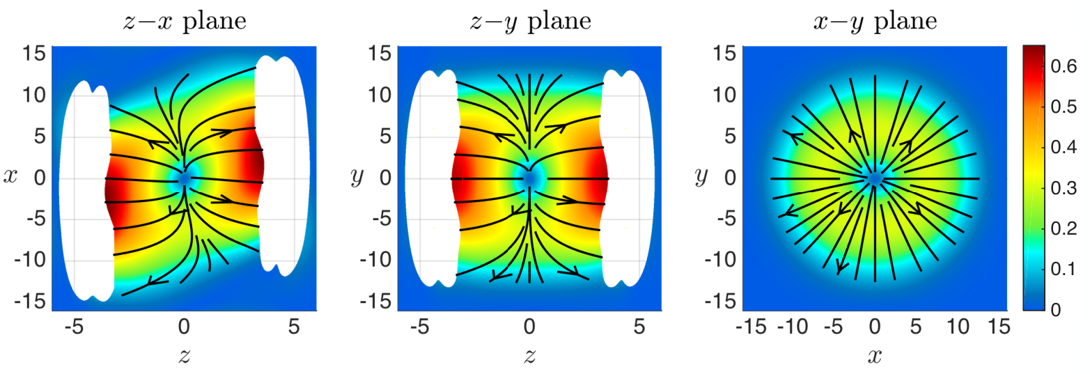
A striking feature of the the post-collision evolution in Fig. 1 is the appearance of flow in the transverse plane at early times. The early-time acceleration imparted on the transverse flow can have a significant impact on the subsequent transverse expansion. In Fig. 4 we plot the fluid 3-velocity in the , , and planes at time . The color scaling, which indicates , is the same in each plot. The flow lines show the direction of . Regions in which , and the system is not behaving hydrodynamically, have been excised. Already at time and radius the transverse fluid velocity in the plane has magnitude 0.3. In contrast, the maximum of the longitudinal velocity, which occurs in the neighborhood of the receding maxima, is 0.64.
One sees from Fig. 4 that the fluid velocity in the plane is nearly radial: we see no strong signatures of elliptic flow. At vanishing rapidity (or ), the traceless part of the spatial stress, as well as the hydrodynamic residual shown in the upper row of fig. 3, deviate significantly from rotational symmetry in the plane (at a 5–6% level at ). However, the energy density and the resulting fluid velocity deviate only slightly from azimuthal symmetry; at their transverse plane anisotropy is about 1%. Our computed evolution does not extend through the entire hydrodynamic phase of the plasma and continued hydrodynamic expansion may generate more elliptic flow. However, the very modest elliptic flow, despite the substantial impact parameter, may reflect an unphysical aspect of our choice of Gaussian initial energy density profiles. Gaussian profiles differ, of course, from more realistic models of nuclear density (such as Wood-Saxon profiles). But a Gaussian profile in the transverse plane is computationally convenient. The very rapid decrease of its Fourier transform allowed us to use a rather modest transverse grid. However, a special feature of Gaussian transverse plane profiles is that the overlap function (i.e., the product of the energy densities of the two incident projectiles) is rotationally symmetric for any impact parameter:
| (11) |
With Gaussian profiles (and equal size incident projectiles), there simply is no “almond” in the overlap function. The actual dynamics depends, of course, on the full spacetime dependence of the initial data, not just on this overlap function and, as noted above, the stress tensor and the residual depart significantly from transverse rotational symmetry. Nevertheless, a simple picture in which the early transverse flow reflects, in large part, this initial overlap function appears plausible.
A notable feature in our results is that the fluid flow, in the plane, is not symmetric about the axis and the longitudinal flow does not vanish at . The latter observation is a direct violation of the simplified model of boost invariant flow, in which and vanishes at . Nevertheless, at and in the region of space where , the longitudinal flow is roughly described by boost invariant flow at the 20% level or better, with larger deviations appearing at larger rapidities.44 4 Specifically, in the region where , we find . For planar shock collisions, the deviation of the longitudinal fluid velocity from boost invariant flow decreases as the shock thickness decreases [11, 4].55 5 However, even in the limit of thin planar shocks the proper energy density has strong rapidity dependence [4, 11]. It will be interesting to see if this also holds when transverse dynamics is included.
We conclude by discussing the early-time transverse flow predicted in ref. [16]. There, using assumptions of boost invariance and transverse plane rotational symmetry, it is argued that at early times the transverse energy flux is proportional to the gradient of the energy density and grows linearly with time,
| (12) |
In Fig. 5 we plot the angular averaged radial flow , together with the approximation (12), at proper times and 2, and rapidities and 1. The approximation (12) works remarkably well at both times and rapidities, although the agreement is not quite as good at where the assumption of boost invariance is more strongly violated. It would be interesting to see if the agreement with the approximation (12) improves when the shock thickness decreases.
4 Final remarks
We have presented results from the first calculation, using numerical holography, of the evolution in strongly coupled SYM theory of an initial state which resembles two colliding heavy nuclei, Correctly treating the dynamics, both longitudinal and transverse, requires solving a five dimensional gravitational initial value problem. This was challenging, but feasible, using our characteristic formulation and (good) desktop-scale computing resources. The results presented above are a proof-of-principle. Clearly, it will be interesting to explore how results change as the impact parameter, longitudinal thickness, and transverse size of each projectile are varied. It should also be possible to explore the effects produced by using more realistic initial energy density profiles, possibly including shorter distance fluctuations of the type which have been suggested to be relevant in real heavy ion collisions. (See, for example, ref. [17, 18, 19, 20] and references therein.) We hope future work will shed light on some of these topics.
Acknowledgements.
We thank Wilke van der Schee for discussions of prior work. The work of PC is supported by the Fundamental Laws Initiative of the Center for the Fundamental Laws of Nature at Harvard University. The work of LY was supported, in part, by the U.S. Department of Energy under Grant No. DE-SC0011637. He thanks the Alexander von Humboldt Foundation and the University of Regensburg for their generous support and hospitality during portions of this work.References
- [1] E. V. Shuryak, “What RHIC experiments and theory tell us about properties of quark-gluon plasma?,” Nucl. Phys. A750 (2005) 64–83, hep-ph/0405066.
- [2] P. M. Chesler and L. G. Yaffe, “Boost invariant flow, black hole formation, and far-from-equilibrium dynamics in supersymmetric Yang-Mills theory,” Phys.Rev. D82 (2010) 026006, arXiv:0906.4426 [hep-th].
- [3] P. M. Chesler and L. G. Yaffe, “Holography and colliding gravitational shock waves in asymptotically AdS5 spacetime,” Phys.Rev.Lett. 106 (2011) 021601, arXiv:1011.3562 [hep-th].
- [4] J. Casalderrey-Solana, M. P. Heller, D. Mateos, and W. van der Schee, “From full stopping to transparency in a holographic model of heavy ion collisions,” Phys.Rev.Lett. 111 (2013) 181601, arXiv:1305.4919 [hep-th].
- [5] W. van der Schee, P. Romatschke, and S. Pratt, “Fully dynamical simulation of central nuclear collisions,” Phys.Rev.Lett. 111 no. 22, (2013) 222302, arXiv:1307.2539.
- [6] H. Bantilan, F. Pretorius, and S. S. Gubser, “Simulation of asymptotically AdS5 spacetimes with a generalized harmonic evolution scheme,” Phys.Rev. D85 (2012) 084038, arXiv:1201.2132 [hep-th].
- [7] H. Bantilan and P. Romatschke, “Simulation of black hole collisions in asymptotically AdS spacetimes,” arXiv:1410.4799 [hep-th].
- [8] S. S. Gubser, S. S. Pufu, and A. Yarom, “Entropy production in collisions of gravitational shock waves and of heavy ions,” Phys. Rev. D78 (2008) 066014, arXiv:0805.1551 [hep-th].
- [9] D. Grumiller and P. Romatschke, “On the collision of two shock waves in AdS5,” JHEP 08 (2008) 027, arXiv:0803.3226 [hep-th].
- [10] S. de Haro, S. N. Solodukhin, and K. Skenderis, “Holographic reconstruction of space-time and renormalization in the AdS / CFT correspondence,” Commun.Math.Phys. 217 (2001) 595–622, arXiv:hep-th/0002230 [hep-th].
- [11] P. M. Chesler and L. G. Yaffe, “Numerical solution of gravitational dynamics in asymptotically anti-de Sitter spacetimes,” JHEP 1407 (2014) 086, arXiv:1309.1439 [hep-th].
- [12] S. Bhattacharyya, V. E. Hubeny, S. Minwalla, and M. Rangamani, “Nonlinear fluid dynamics from gravity,” JHEP 02 (2008) 045, arXiv:0712.2456.
- [13] R. Baier, P. Romatschke, D. T. Son, A. O. Starinets, and M. A. Stephanov, “Relativistic viscous hydrodynamics, conformal invariance, and holography,” JHEP 0804 (2008) 100, arXiv:0712.2451 [hep-th].
- [14] M. P. Heller, D. Mateos, W. van der Schee, and D. Trancanelli, “Strong coupling isotropization of non-Abelian plasmas simplified,” Phys.Rev.Lett. 108 (2012) 191601, arXiv:1202.0981 [hep-th].
- [15] M. P. Heller, D. Mateos, W. van der Schee, and M. Triana, “Holographic isotropization linearized,” JHEP 1309 (2013) 026, arXiv:1304.5172 [hep-th].
- [16] J. Vredevoogd and S. Pratt, “Universal flow in the first stage of relativistic heavy ion collisions,” Phys.Rev. C79 (2009) 044915, arXiv:0810.4325 [nucl-th].
- [17] M. Luzum and H. Petersen, “Initial state fluctuations and final state correlations in relativistic heavy-ion collisions,” J.Phys. G41 (2014) 063102, arXiv:1312.5503 [nucl-th].
- [18] S. Floerchinger and U. A. Wiedemann, “Statistics of initial density perturbations in heavy ion collisions and their fluid dynamic response,” JHEP 1408 (2014) 005, arXiv:1405.4393 [hep-ph].
- [19] B. Schenke, P. Tribedy, and R. Venugopalan, “Initial-state geometry and fluctuations in Au + Au, Cu + Au, and U + U collisions at energies available at the BNL Relativistic Heavy Ion Collider,” Phys.Rev. C89 no. 6, (2014) 064908, arXiv:1403.2232 [nucl-th].
- [20] C. Shen, Z. Qiu, and U. Heinz, “Shape and flow fluctuations in ultra-central Pb+Pb collisions at the LHC,” arXiv:1502.04636 [nucl-th].