Proper affine deformations of two-generator Fuchsian groupsThanks: Charette gratefully acknowledges partial support from the Natural Sciences and Engineering Research Council of Canada. Goldman gratefully acknowledges partial support from National Science Foundation grant DMS070781. All three authors acknowledge support from U.S. National Science Foundation grants DMS 1107452, DMS1107263, DMS 1261522 and ,in particular DMS1107367 “Research Networks in the Mathematical Sciences: Geometric structures And Representation varieties” (the GEAR Network) to facilitate this research.

By a triple (respectively pair) we shall always mean an ordered triple or pair respectively, unless otherwise stated.

The complement of a subset $X$ will sometimes be denoted $X^{c}$.

Denote the ring of rational integers by $\mathbb{Z}$ and the fields of rational, real and complex numbers by $\mathbb{Q},\mathbb{R}$ and $\mathbb{C}$ respectively. The multiplicative groups of nonzero (respectively positive) real numbers will be denoted $\mathbb{R}^{*}$ (respectively $\mathbb{R}_{+}$).

If $A$ is an element of a group, denote by $\langle A\rangle$ the cyclic subgroup generated by $A$.

If $A,B$ are invertible transformations, denote the commutator by:

and conjugation by:

For any group $G$, denote its identity element as $\mathbb{I}$, the inverse operation as $g\longmapsto g^{-1}$ and its multiplication by $(a,b)\longmapsto ab$. Denote its automorphism group by $\mathsf{Aut}(G)$. Denote its normal subgroup of inner automorphisms by $\mathsf{Inn}(G)$ and the quotient $\mathsf{Aut}(G)/\mathsf{Inn}(G)$ by $\mathsf{Out}(G)$.

If $V$ is a vector space over a field $k$, and $\mathbf{v}\in V$ is a vector, denote $k\mathbf{v}$ the $1$-dimensional linear subspace spanned by $\mathbf{v}$. The projective space $\mathsf{P}(V)$ associated to $V$ is the set of all lines

where $\mathbf{v}\neq 0$. Defined the projectivization mapping by:

Projectivization is the quotient map for action of $\mathbb{R}^{*}$ by homotheties. Since $\mathbb{R}^{*}=\mathbb{R}_{+}\times\{\pm 1\}$, projectivization factors as the composition of two quotient maps, one by the group of positive scalings $\mathbb{R}_{+}$ and one by $\{\pm 1\}$. The sphere of directions $\mathsf{S}(V)$, the set of rays at $0$ in $V$, is the quotient space $\big(V\setminus\{0\}\big)/\mathbb{R}_{+}$. The $\{\pm 1\}$-quotient map $\mathsf{S}(V)\longrightarrow\mathsf{P}(V)$ is a double covering with covering group $\{\pm 1\}$. Given a Euclidean structure on $V$, its unit sphere is a covenient cross-section to the $\mathbb{R}_{+}$-quotient map $V\setminus\{0\}\longrightarrow\mathsf{S}(V)$. This sphere $\mathsf{S}(V)$ double covers $\mathsf{P}(V)$ with covering group $\{\pm 1\}$.

The notation for surfaces follows [22]. An $n$-holed orientable surface of genus $g$ is denoted $\Sigma_{g,n}$. Such a surface is represented as the complement of $n$ disjoint discs in a connected sum $\Sigma_{g}$ of $g$ tori (each summand is $\Sigma_{1,0}$ and $\Sigma_{0}$ is a $2$-sphere). Similarly, $C_{g,n}$ is represented as the complement of $n$ disjoint discs in a connected sum of $g$ cross-surfaces. (A cross-surface is the name proposed by John H. Conway for a topological space homeomorphic to the real projective plane.)

Let $\Sigma$ be a surface with boundary $\partial\Sigma$. A closed simple curve on $\Sigma$ is essential if and only if it is not homotopic to a point. A simple closed curve is peripheral if and only if it is homotopic to a curve in $\partial\Sigma$. If $\partial\Sigma$ is connected, then a simple closed curve is nonseparating if and only if it essential and nonperipheral. (This simply means its complement is connected.) By a curve class we shall mean an isotopy class of essential nonperipheral simple closed curves. In particular the curves are not assumed to be oriented, and the isotopies are not required to preserve a (so far unmentioned) basepoint. Denote the set of curve classes by $\mathscr{S}$. Denote the set of isotopy class of oriented essential nonperipheral simple closed curves by $\mathscr{S}^{+}$.

If $\alpha,\beta\in\mathscr{S}$, their geometric intersection number $i(\alpha,\beta)$ is the nonnegative integer which is the minimum cardinality of intersections of representative curves in $\alpha,\beta$ respectively. If $\Sigma$ is given a hyperbolic structure, then $i(\alpha,\beta)$ equals the cardinality of the intersection of the unique closed geodesics representing $\alpha$ and $\beta$ (unless $\alpha=\beta$ in which case $i(\alpha,\beta)=0$).

The mapping class group of $\Sigma$ is defined as the group of isotopy classes of homeomorphisms of $\Sigma$:

Note that we do not restrict to orientation-preserving homeomorphisms, and $\mathsf{Mod}(\Sigma)$ is therefore defined even when $\Sigma$ is nonorientable.

An affine space is a set equipped by a simply transitive action of a vector space. We denote the affine space by $\mathsf{E}$ and the vector space by $\mathsf{V}$. The elements of $\mathsf{E}$ are points, and the elements of $\mathsf{V}$ are vectors. Vectors $\mathbf{v}\in\mathsf{E}$ identify with transformations $\mathsf{E}\longrightarrow\mathsf{E}$, the translations. If $p\in\mathsf{E}$ is a point and $\mathbf{v}\in\mathsf{V}$ is a vector, then the effect of translation by $\mathbf{v}$ on $p$ is the point which we denote $p+\mathbf{v}$. We denote the unique vector effecting the translation taking point $p$ to point $q$ by $q-p\in\mathsf{V}$; this is just the vector difference in standard coordinates derived from a basis of $\mathsf{V}$.

In this paper, all vector spaces are vector spaces over the field $\mathbb{R}$ of real numbers. Then $\mathsf{E}$ is a smooth manifold and the simply transitive action of $\mathsf{V}$ on $\mathsf{E}$ identifies $\mathsf{V}$ with each tangent space $\mathsf{T}_{p}\mathsf{E}$ for each point $p\in\mathsf{E}$. If $[a,b]\xrightarrow{\gamma}\mathsf{E}$ is a smooth curve in affine space, then for each parameter $t\in[a,b]$, the velocity vector

is defined. The differential-geometric context is the following: $\mathsf{E}$ is a smooth $1$-connected manifold with a geodesically complete flat torsionfree affine connection. Conversely, every $1$-connected smooth manifold with geodesically complete flat torsionfree affine connection is isomorphic to such an affine space.

When $\mathsf{V}$ is equipped with a positive definite inner product, the affine space $\mathsf{E}$ is Euclidean space. A Riemannian manifold $(M,g)$ is isometric to a Euclidean space $\mathsf{E}$ if and only if $M$ is $1$-connected, and the Riemannian metric $g$ is geodesically complete and has zero curvature and torsion.

In this paper, $\mathsf{V}$ will be a Lorentzian vector space, that is, a $3$-dimensional inner product space of signature $(2,1)$. We denote the inner product of two vectors $\mathbf{v},\mathbf{u}\in\mathsf{V}$ by $\mathbf{v}\cdot\mathbf{u}$. (We emphasize this notation is not the usual Euclidean dot product.) When the $\mathsf{V}$ is oriented, the associated cross product

is unambiguously defined by

(Here $\mathsf{Det}$ is the alternating trilinear form on $\mathsf{V}$, uniquely specified by having unit length with respect to the induced inner product on $\Lambda^{3}(\mathsf{V})^{*}$ and compatible with the chosen orientation on $\mathsf{V}$.)

The following standard identity will be useful later:

Define Minkowski space as an affine space $\mathsf{E}$ whose underlying vector space $\mathsf{V}$ has the structure of a Lorentzian vector space. Alternatively, $\mathsf{E}$ is a geodesically complete $1$-connected flat Lorentzian manifold.

The geodesics in $\mathsf{E}$ are just Euclidean straight lines, parametrized at constant Euclidean speed:

Depending on whether the (constant) velocity vector $\mathbf{v}$ is timelike, null, or spacelike, we say the geodesic is a particle, photon, or tachyon, respectively.

The group of all isometries of Minkowski space $\mathsf{E}$ splits as a semidirect product $\mathsf{O}(2,1)\ltimes\mathsf{V}$ where now $\mathsf{V}$ denotes the vector space of translations. Its index-two subgroup of orientation-preserving isometries $\mathsf{Isom}^{+}(\mathsf{E})$ is the semidirect product ${\mathsf{SO}(2,1)}\ltimes\mathsf{V}$, that is, the following sequence of groups

is exact.

Suppose that $\mathbf{u}\in\mathsf{V}$ is a vector which is not null. Then

defines an involution of $\mathsf{V}$ fixing $\mathbf{u}$ having $\mathbf{u}^{\perp}$ as its $(-1)$-eigenspace. For timelike $\mathbf{u}$, this involution defines the symmetry of $\mathsf{H}^{2}$ in the corresponding point in $\mathsf{H}^{2}$; for spacelike $\mathbf{u}$, this involution defines reflection in the corresponding geodesic in $\mathsf{H}^{2}$.

Let $T:=p+\mathbb{R}\mathbf{t}$ be a particle parallel to a unit-timelike vector $\mathbf{t}\in\mathsf{V}$ (that is, $\mathbf{t}\cdot\mathbf{t}=-1$). The corresponding reflection is:

Let $\mathsf{V}$ be an oriented Lorentzian vector space. The hyperbolic plane $\mathsf{H}^{2}$ is defined as the subset of the projective space $\mathsf{P}(\mathsf{V})$ consisting of timelike lines (particles), that is, lines spanned by vectors $\mathbf{t}$ such that $\mathbf{t}\cdot\mathbf{t}<0$.

The set of all nonzero non-spacelike vectors (that is, vectors $\mathbf{v}\neq 0$ such that $\mathbf{v}\cdot\mathbf{v}\leq 0$) falls into two components, denoted $\mathsf{Future}$ and $\mathsf{Past}$. The choice of a component $\mathsf{Future}$ is equivalent to choosing a time-orientation on $\mathsf{V}$ and is useful in discussing the Riemannian metric and the orientation of $\mathsf{H}^{2}$. Namely, we identify $\mathsf{H}^{2}$ with

The Lorentzian structure on $\mathsf{V}$ induces a Riemannian metric on $\mathsf{H}^{2}$ of constant curvature $-1$. Furthermore the orientation on $\mathsf{V}$ and the radial vector field on $\mathsf{V}$ induce an orientation on $\mathsf{H}^{2}$, when $\mathsf{H}^{2}$ is described as above. However, identifying $\mathsf{H}^{2}$ with the past vectors $\mathbf{t}\in\mathsf{Past}$ satisfying $\mathbf{t}\cdot\mathbf{t}=-1$ gives $\mathsf{H}^{2}$ the opposite orientation.

The group ${\mathsf{SO}(2,1)}$ of orientation-preserving linear isometries of $\mathsf{V}$ isometrically on $\mathsf{H}^{2}$ as follows. Its identity component ${\mathsf{SO}(2,1)^{0}}$ preserves $\mathsf{Future}$ and acts by orientation-preserving isometries of $\mathsf{H}^{2}$. (Here $\mathsf{H}^{2}$ inherits an orientation from $\mathsf{V}$ and the radial vector field on $\mathsf{V}$.) However, orientation-preserving linear isometries of $\mathsf{V}$ not in ${\mathsf{SO}(2,1)^{0}}$ interchange $\mathsf{Future}$ and $\mathsf{Past}$.

Here is how we interpret $\mathsf{H}^{2}$ in terms of the affine Lorentzian geometry of Minkowski space $\mathsf{E}$. The translations of $\mathsf{E}$ act on particles (timelike geodesics) in $\mathbf{t}\subset\mathsf{E}$. Points in $\mathsf{H}^{2}$ then correspond to translational equivalence classes of particles in $\mathsf{E}$. We denote the equivalence class of $\mathbf{t}$ as $[\mathbf{t}]\in\mathsf{H}^{2}$. Similarly, points of $\partial\mathsf{H}^{2}$ correspond to translational equivalence classes of null geodesics in $\mathsf{V}$ and geodesics in $\mathsf{H}^{2}$ correspond to translational equivalence classes of tachyons (spacelike geodesics) in $\mathsf{E}$. See [2] for further details.

Geodesics in $\mathsf{H}^{2}$ correspond to spacelike $1$-dimensional linear subspaces of $\mathsf{V}$. Oriented geodesics in $\mathsf{H}^{2}$ correspond to unit-spacelike vectors. The projectivization $\mathsf{P}(\mathbf{v}^{\perp})$ of the orthogonal complement $\mathbf{v}^{\perp}$ of a spacelike vector $\mathbf{v}\in\mathsf{V}$ meets $\mathsf{P}(\mathsf{V}_{-})\approx\mathsf{H}^{2}$ in a geodesic. A geodesic in $\mathsf{H}^{2}$ separates $\mathsf{H}^{2}$ into two halfplanes.

Time-orientations of $\mathsf{V}$ can be used to conveniently parametrize halfplanes in $\mathsf{H}^{2}$, as follows. Choose a connected component $\mathsf{Future}$ of

Then $\mathsf{P}(\mathsf{Future})=\mathsf{H}^{2}$ and restriction of the quotient map

identifies $\mathsf{H}^{2}$ with

Under this identification, a spacelike vector $\mathbf{s}$ determines a halfplane:

bounded by the geodesic $\mathsf{P}(\mathbf{s}^{\perp})$. The complement of the geodesic $\mathsf{P}(\mathbf{s}^{\perp})$ consists of the interiors of the two halfplanes $\mathcal{H}(\mathbf{s})$ and $\mathcal{H}(-\mathbf{s})$.

The time-orientation on $\mathsf{V}$ (together with the orientation on $\mathsf{V}$) induces an orientation on $\mathsf{H}^{2}$. In this way an oriented geodesic $l\subset\mathsf{H}^{2}$ determines a halfplane bounded by $l$.

Define an ideal polygon $\Pi$ in $\mathsf{H}^{2}$ as a closed submanifold-with-boundary in $\mathsf{H}^{2}$ whose boundary is a disjoint union of complete mutually asymptotic geodesics, which we call its sides. The complement of an ideal polygon is a disjoint union of (open) halfplanes, and each side bounds a halfplane. If $\Pi$ is finite-sided, then the union of $\Pi$ with the set of endpoints of its sides is compact.

An ideal triangle is an ideal polygon with three sides and an ideal quadrilateral is an ideal polygon with four sides. A pointed ideal polygon is an ideal polygon with a choice of a point on each one of its sides.

For hyperbolic $X$, denote by ${X}^{+},{X}^{-}$ respectively its attracting and repelling fixed points. When $X$ is parabolic, then denote by ${X}^{+}={X}^{-}$ its single fixed point. If $X,Y\in{\mathsf{SO}(2,1)^{0}}$ and $X$ is hyperbolic or parabolic, then

A discrete group $\Gamma_{0}$ of isometries of $\mathsf{H}^{2}$ acts properly on $\mathsf{H}^{2}$. Furthermore a discrete group $\Gamma_{0}$ acts freely if and only if $\Gamma_{0}$ is torsionfree. The quotient $\Sigma=\mathsf{H}^{2}/\Gamma_{0}$ is a complete hyperbolic surface with fundamental group isomorphic to $\Gamma_{0}$.

Let $x\in\mathsf{H}^{2}$. Then the closure of the orbit $\Gamma_{0}(x)$ in $\mathsf{H}^{2}\cup\partial\mathsf{H}^{2}$ is independent of $x$, and is called the limit set of $\Gamma_{0}$, and denoted $\Lambda$. If $\Gamma_{0}$ is nonelementary, that is, not virtually abelian, then $\Lambda$ is the unique minimal closed $\Gamma_{0}$-invariant subset of $\partial\mathsf{H}^{2}$. Geodesic rays in $\mathsf{H}^{2}$ approaching a point of $\Lambda$ project to nonwandering (or weakly recurrent) geodesic rays on the quotient.

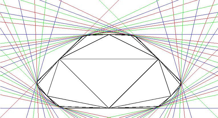
The Nielsen convex region of $\Gamma_{0}$ is the convex hull $\mathsf{Hull}(\Lambda)$ of $\Lambda$ in $\mathsf{H}^{2}$. Its quotient, the convex core $\mathsf{Core}(\Sigma)$, is the unique minimal convex subsurface carrying $\pi_{1}(\Sigma)$: Any geodesically convex subsurface $\Sigma^{\prime}\subset\Sigma$ such that the inclusion $\Sigma^{\prime}\hookrightarrow\Sigma$ is a homotopy equivalence must contain $\mathsf{Core}(\Sigma)$. Figure 1 depicts a Nielsen convex region in $\mathsf{H}^{2}$, tiled by ideal triangles.

Consider a Fuchsian group $\Gamma_{0}\subset{\mathsf{SO}(2,1)}$ which is free of rank two. Denote the embedding onto $\Gamma_{0}$ by:

An affine deformation of $\Gamma_{0}$ is a lift $\rho$ of $\rho_{0}$, namely a homomorphism such that $\rho_{0}=\mathsf{L}\circ\rho$, that is, such that the diagram

commutes, Translational conjugacy classes of affine deformations form the vector space $H^{1}(\mathsf{F}_{2},\mathsf{V})$, where $\mathsf{V}$ is the $\mathsf{F}_{2}$-module defined by the representation $\mathsf{F}_{2}\hookrightarrow{\mathsf{SO}(2,1)}$. Explicitly, $\rho=(\rho_{0},u)$, where $\mathsf{F}_{2}\xrightarrow{u}\mathsf{V}$ is the translational part:

then $u\in Z^{1}(\mathsf{F}_{2},\mathsf{V})$ is a cocycle taking values in the $\mathsf{F}_{2}$-module defined by $\rho_{0}$.

In this paper, we will work in a more geometric context, where Margulis spacetimes are affine deformations of the hyperbolic surface $\Sigma$. Equivalently, $\rho_{0}$ corresponds to the marked hyperbolic surface

with an isomorphism $\pi_{1}(\Sigma_{0})\cong\mathsf{F}_{2}$. This isomorphism induces an isomorphism

and the cohomology space $H^{1}(\Sigma_{0},\mathsf{V})$ is the space of all affine deformations of the hyperbolic surface $\Sigma_{0}$.

A basis of $\mathsf{F}_{2}$ is an ordered pair $(A,B)\in\mathsf{F}_{2}\times\mathsf{F}_{2}$ such that $A$ and $B$ generate $\mathsf{F}_{2}$. (Necessarily $A$ and $B$ freely generate $\mathsf{F}_{2}$.) Denote the set of bases of $\mathsf{F}_{2}$ by $\mathsf{Basis}(\mathsf{F}_{2})$. A basic triple is an ordered triple

with $ABC=\mathbb{I}$, such that $(A,B)\in\mathsf{Basis}(\mathsf{F}_{2})$. Clearly bases extend uniquely to basic triples by defining $C:=B^{-1}A^{-1}$. Conversely any pair inside a basic triple is a basis.

The automorphism group $\mathsf{Aut}(\mathsf{F}_{2})$ acts simply transitively on $\mathsf{Basis}(\mathsf{F}_{2})$: if $(A_{0},B_{0})\in\mathsf{Basis}(\mathsf{F}_{2})$ and $(A,B)\in\mathsf{F}_{2}\times\mathsf{F}_{2}$, then the mapping

extends uniquely to an endomorphism $\mathsf{F}_{2}\longrightarrow\mathsf{F}_{2}$. This endomorphism is an automorphism if and only if $(A,B)\in\mathsf{Basis}(\mathsf{F}_{2}).$

An element $A\in\mathsf{F}_{2}$ is primitive if and only if $A$ extends to a basis. Let $\mathsf{Prim}(\mathsf{F}_{2})\subset\mathsf{F}_{2}$ denote the set of primitives in $\mathsf{F}_{2}$. If $A\in\mathsf{Prim}(\mathsf{F}_{2})$, then the set of elements $B\in\mathsf{F}_{2}$ such that $(A,B)\in\mathsf{Basis}(\mathsf{F}_{2})$ is the double coset $\langle A\rangle B_{0}\langle A\rangle$ where $B_{0}$ is an arbitrary element of this set.

The group $\mathsf{Inn}(\mathsf{F}_{2})\cong\mathsf{F}_{2}$ of inner automorphisms acts on the set $\mathsf{Prim}(\mathsf{F}_{2})$. We find a double extension $\mathsf{Inn}^{\mathfrak{e}}(\mathsf{F}_{2})$ of $\mathsf{Inn}(\mathsf{F}_{2})$ such that the quotient $\mathsf{Prim}(\mathsf{F}_{2})/\mathsf{Inn}^{\mathfrak{e}}(\mathsf{F}_{2})$ identifies with the set $\mathscr{S}$ of free isotopy classes of unoriented noseparating simple closed curves on $\Sigma$.

The set $\mathsf{Prim}(\mathsf{F}_{2})/\mathsf{Inn}^{\mathfrak{e}}\cong\mathbb{Q}\mathsf{P}^{1}$ enjoys a rich combinatorial structure which we encode in a trivalent tree $\mathsf{T}$ with a $\mathsf{GL(2,\mathbb{Z})}$-action. In §6 this will be related to topological objects on $\Sigma$.

Superbases arise in several closely related contexts dealing with $\mathsf{F}_{2}$; in particular, superbases describe affine coordinate systems on deformation spaces of $\mathsf{SL}(2)$-representations of $\mathsf{F}_{2}$. They will also parametrize the affine deformations, and also the tiles in the affine deformation space which correspond to ideal triangulations of a hyperbolic surface $\Sigma\approx\Sigma_{1,1}$. After defining superbases in §5.4.1, we explain their combinatorial structure, which appears in the proper affine deformation space. Specifically, the set of unordered superbases defines the set of vertices of a binary trivalent tree, with edges corresponding to the relation of neighboring superbases.

The previous discussion of superbases in $\mathbb{Z}^{2}$ motivates the present discussion. Farey triples in $\mathbb{Q}\mathsf{P}^{1}$ precisely correspond to superbases in $\mathsf{F}_{2}$, our principal object of study.

The key point is the following. If $(A,B)\in\mathsf{Basis}(\mathsf{F}_{2})$ is a basis, then $\big(\mathscr{A}(A),\mathscr{A}(B)\big)$ is a basis of the free abelian group $\mathbb{Z}^{2}$ and the corresponding points are Farey neighbors in $\mathbb{Q}\mathsf{P}^{1}$. Conversely, a pair of Farey neighbors in $\mathbb{Q}\mathsf{P}^{1}$ determines a basis of $\mathsf{F}_{2}$, unique up to the action of $\mathsf{Inn}^{\mathfrak{e}}$.

References

- [1] Herbert Abels, Properly discontinuous groups of affine transformations: A survey, Geometriae Dedicata 87 (2001), no. 1-3, 309–333.
- [2] Jean-Philippe Burelle, Virginie Charette, Todd A. Drumm, and William M. Goldman, Crooked halfspaces, Enseign. Math. 60 (2014), no. 1, 43–78. MR 3262435
- [3] Bruce Chandler and Wilhelm Magnus, The history of combinatorial group theory, Studies in the History of Mathematics and Physical Sciences, vol. 9, Springer-Verlag, New York, 1982, A case study in the history of ideas. MR 680777 (85c:01001)
- [4] Virginie Charette, Affine deformations of ultraideal triangle groups, Geometriae Dedicata 97 (2003), no. 1, 17–31.
- [5] by same author, The affine deformation space of a rank two Schottky group: a picture gallery, Geom. Dedicata 122 (2006), 173–183. MR 2295549 (2008b:20061)
- [6] by same author, Non-proper affine actions of the holonomy group of a punctured torus, Forum Mathematicum 18 (2006), no. 1, 121–135.
- [7] Virginie Charette and Todd A. Drumm, Strong marked isospectrality of affine Lorentzian groups, J. Differential Geom. 66 (2004), no. 3, 437–452. MR 2106472 (2006b:53053)
- [8] by same author, The Margulis invariant for parabolic transformations, Proc. Amer. Math. Soc. 133 (2005), no. 8, 2439–2447. MR 2138887 (2005m:53011)
- [9] Virginie Charette, Todd A. Drumm, and William M. Goldman, Affine deformations of a three-holed sphere, Geom. Topol. 14 (2010), no. 3, 1355–1382. MR 2653729 (2011e:57027)
- [10] Virginie Charette, Todd A. Drumm, and William M Goldman, Finite-sided deformation spaces of complete affine 3-manifolds, Journal of Topology 7 (2014), no. 1, 225–246.
- [11] Virginie Charette and William M. Goldman, Affine Schottky groups and crooked tilings, in Igodt et al. [26], pp. 69–97. MR 1796126 (2001j:57047)
- [12] Suhyoung Choi and William M. Goldman, Topological tameness of Margulis spacetimes, arXiv preprint arXiv:1204.5308, 2013.
- [13] John H. Conway, The sensual (quadratic) form, Carus Mathematical Monographs, vol. 26, Mathematical Association of America, Washington, DC, 1997, With the assistance of Francis Y. C. Fung. MR 1478672 (98k:11035)
- [14] Jeffrey Danciger, François Guéritaud, and Fanny Kassel, Geometry and topology of complete Lorentz spacetimes of constant curvature, arXiv preprint arXiv:1306.2240, (2013), to appear in Annales Scientifiques de l’École Normale Supérieur.
- [15] by same author, Margulis spacetimes via the arc complex, arXiv preprint arXiv:1407.5422v1, 2013.
- [16] Todd A. Drumm, Fundamental polyhedra for Margulis space-times, Ph.D. thesis, University of Maryland, 1990.
- [17] Todd A Drumm, Fundamental polyhedra for Margulis space-times, Topology 31 (1992), no. 4, 677–683.
- [18] Todd A. Drumm, Linear holonomy of Margulis space-times, J. Differential Geom 38 (1993), no. 3, 679–690.
- [19] Todd A Drumm and William M Goldman, The geometry of crooked planes, Topology 38 (1999), no. 2, 323–351.
- [20] Todd A. Drumm and William M. Goldman, Isospectrality of flat Lorentz 3-manifolds, Journal of Differential Geometry 58 (2001), no. 3, 457–465.
- [21] William M Goldman, The Margulis invariant of isometric actions on Minkowski (2+ 1)-space, Rigidity in Dynamics and Geometry, Springer, 2002, pp. 187–201.
- [22] William M. Goldman, Trace coordinates on Fricke spaces of some simple hyperbolic surfaces, Handbook of Teichmüller theory. Vol. II, IRMA Lect. Math. Theor. Phys., vol. 13, Eur. Math. Soc., Zürich, 2009, pp. 611–684. MR 2497777 (2010j:30093)
- [23] William M. Goldman, François Labourie, and Gregory Margulis, Proper affine actions and geodesic flows of hyperbolic surfaces, Ann. of Math. (2) 170 (2009), no. 3, 1051–1083. MR 2600870 (2011b:30109)
- [24] William M. Goldman, François Labourie, Gregory Margulis, and Yair Minsky, Complete flat Lorentz -manifolds and laminations on hyperbolic surfaces, in preparation.
- [25] William M. Goldman and Gregory A. Margulis, Flat Lorentz 3-manifolds and cocompact Fuchsian groups, in Igodt et al. [26], pp. 135–145. MR 1796129 (2001m:53124)
- [26] Paul Igodt, Herbert Abels, Yves Félix, and Fritz Grunewald (eds.), Crystallographic groups and their generalizations, Contemporary Mathematics, vol. 262, American Mathematical Society, Providence, RI, 2000. MR 1796123 (2001e:00018)
- [27] François Labourie, Fuchsian affine actions of surface groups, J. Differential Geom. 59 (2001), no. 1, 15–31. MR 1909247 (2003d:57061)
- [28] Gregory Margulis, Free properly discontinuous groups of affine transformations, Dokl. Akad. Nauk SSSR 272 (1983), no. 4, 937–940.
- [29] by same author, Complete affine locally flat manifolds with a free fundamental group, Journal of Soviet Mathematics 36 (1987), no. 1, 129–139.
- [30] Geoffrey Mess, Lorentz spacetimes of constant curvature, Geometriae Dedicata 126 (2007), no. 1, 3–45.
- [31] J. Nielsen, Die isomorphismengruppe der allgemeinen unendlichen gruppe mit zwei erzeugenden, Math. Ann. 78 (1917), 385–397.
- [32] H. Vogt, Sur les invariants fondamentaux des équations différentielles linéaires du second ordre, Annales Scientifiques de l’École Normale Supérieure 6 (1889), 3–71.