跳到论文正文
W Papers独立论文阅读器 arXiv:1501.04455 论文正文 计算阅读时间 · 0%
引用这篇论文根据当前论文元数据生成,正式投稿前建议核对。


License: arXiv.org perpetual non-exclusive license
arXiv:1501.04455v2 [hep-ph] 21 Jul 2015

KUNS-2538, OU-HET/850 Eternal Higgs inflation and
cosmological constant problem

Yuta Hamada,  Hikaru Kawai,  and Kin-ya Oda*†Department of Physics, Kyoto University, Kyoto 606-8502, Japan ††thanks: E-mail: hamada@gauge.scphys.kyoto-u.ac.jp††thanks: E-mail: hkawai@gauge.scphys.kyoto-u.ac.jp††thanks: E-mail: odakin@phys.sci.osaka-u.ac.jp Affiliation: Department of Physics, Osaka University, Osaka 560-0043, Japan
August 24, 2026
Abstract

We investigate the Higgs potential beyond the Planck scale in the superstring theory, under the assumption that the supersymmetry is broken at the string scale. We identify the Higgs field as a massless state of the string, which is indicated by the fact that the bare Higgs mass can be zero around the string scale. We find that, in the large field region, the Higgs potential is connected to a runaway vacuum with vanishing energy, which corresponds to opening up an extra dimension. We verify that such universal behavior indeed follows from the toroidal compactification of the non-supersymmetric S​O​(16)×S​O​(16)SO(16)\times SO(16) heterotic string theory. We show that this behavior fits in the picture that the Higgs field is the source of the eternal inflation. The observed small value of the cosmological constant of our universe may be understood as the degeneracy with this runaway vacuum, which has vanishing energy, as is suggested by the multiple point criticality principle.

1 Introduction

The Higgs boson discovered at the LHC [1, 2] beautifully fits into the Standard Model (SM) predictions so far [3]. The determination of its mass [4]

MH\displaystyle M_{H} =125.7±0.4​GeV\displaystyle=125.7\pm 0.4\,\text{GeV} (1)

completes the list of the SM parameters, among which the ones in the Higgs potential,

V\displaystyle V =m2​|H|2+λ​|H|4,\displaystyle=m^{2}\left|H\right|^{2}+\lambda\left|H\right|^{4}, (2)

have turned out to be m2∼−(90​GeV)2m^{2}\sim-\left(90\,\text{GeV}\right)^{2} and λ≃0.13\lambda\simeq 0.13, depending on the precise values of the top and Higgs masses; see e.g. Ref. [5].

We have not seen any hint of a new physics beyond the SM at the LHC, and it is important to guess at what scale it appears, as we know for sure that it must be somewhere in order to account for the tiny neutrino masses, dark matter, baryogenesis, inflation, etc. In this work, we assume that the Higgs sector is not altered up to a very high scale,11 1 See e.g. Refs. [6, 7, 8, 9, 10, 11, 12] for a possible minimal extension of the SM with the dark matter and right-handed neutrinos. in accordance with the following indications: The renormalization group (RG) running of the quartic coupling λ\lambda revealed that it takes the minimum value at around the Planck scale ∼1018​GeV\sim 10^{18}\,\text{GeV} and that the minimum value can be zero depending on the precise value of the top quark mass [13, 14, 15, 16, 17, 18, 19, 20, 21, 5, 22, 23, 24, 25, 26, 27]. We have also found that the bare Higgs mass can vanish at the Planck scale as well [18, 19, 20, 28, 21, 29, 30, 31].22 2 See also Refs. [32, 33, 34] for discussion of quadratic divergences. That is, the Veltman condition [35] can be met at the Planck scale. In fact he speculates, “This mass-relation, implying a certain cancellation between bosonic and fermionic effects, would in this view be due to an underlying supersymmetry.” To summarize, it turned out that there is a triple coincidence: λ\lambda, its running, and the bare Higgs mass can all be accidentally small at around the Planck scale.

This is a direct hint for Planck scale physics in the context of superstring theory. The vanishing bare Higgs mass implies that the supersymmetry is restored at the Planck scale and that the Higgs field resides in a massless string state. The smallness of both λ\lambda and its beta function is consistent with the Higgs potential being very flat around the string scale; see Fig. 1.33 3 This is indeed suggested by the multiple point criticality principle (MPP) [36, 37, 38], the classical conformality [39, 40, 39, 41, 42, 43, 44, 45, 46, 47, 48, 49, 50], the asymptotic safety [51], the hidden duality and symmetry [52, 53], and the maximum entropy principle [54, 55, 56, 57, 58]. Such a flat potential opens up the possibility that the Higgs field plays the role of inflaton in the early universe [59, 60, 61, 62, 63, 64, 65, 66, 67].44 4 There are different models of the Higgs inflation involving higher dimensional operators [68, 69, 70, 71, 72].
Refer to caption

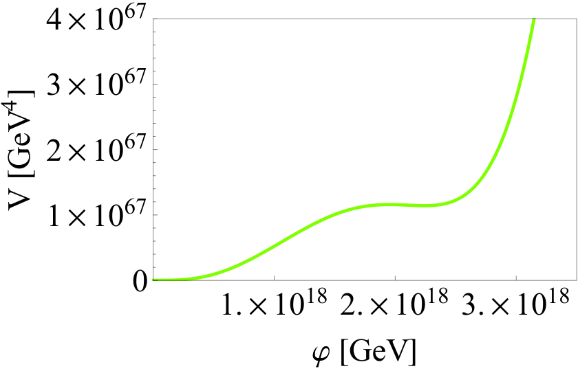
Figure 1: The SM Higgs potential VV as a function of the Higgs field φ\varphi. Here we take MH=125​GeVM_{H}=125\,\text{GeV} and tune the top mass in such a way that the potential becomes flat; see e.g. Ref. [65].

To understand the whole structure of the potential, it is crucial to investigate its behavior beyond the Planck scale. The calculation based on field theory cannot be trusted in this region. Although it is hard to reproduce the SM completely as a low energy effective theory of superstring, we can explore generic trans-Planckian structure of the Higgs field, under the assumption that the SM is close to a non-supersymmetric perturbative vacuum of superstring theory.

In four dimensions, string theory has many more tachyon-free non-supersymmetric vacua than the supersymmetric ones. The latest LHC results suggest the possibility of the absence of the low energy supersymmetry, and the research based on the non-supersymmetric vacua is becoming more and more important [73, 74, 75, 76, 77].

In such non-supersymmetric vacua, almost all the moduli are lifted up perturbatively, contrary to the supersymmetric ones which typically possess tens or even hundreds of flat directions that cannot be raised purturbatively. However, there remains a problem of instability in the non-supersymmetric models: The perturbative corrections generate tadpoles for the dilaton and other moduli such as the radii of toroidal compactifications. The dilaton can be stabilized within the perturbation series when gs∼1g_{s}\sim 1 [78], or else by the balance between the one-loop and the non-perturbative potentials when gsg_{s} is small [77]. In this paper, we assume that the dilaton is already stabilized. We will discuss other instabilities than the dilaton direction in Sections 2 and 3.

We start from the tachyon-free non-supersymmetric vacua of the heterotic string theory. We assume that the Higgs comes from a closed string and that its emission vertex at the zero momentum can be decomposed into a product of operators whose conformal dimensions are (1,0)(1,0) and (0,1)(0,1). This is realized in the following cases for example:

  • •

    The Higgs comes from an extra dimensional component of a gauge field [79, 80, 81, 82, 83, 84, 85].

  • •

    The Higgs is the only one doublet in generic fermionic constructions [86, 87, 88, 89].

  • •

    The Higgs comes from an untwisted sector in the orbifold construction [90, 91]; see e.g. Ref. [73] for a recent model-building example.55 5 In Ref. [73] the SM-like one Higgs doublet model is constructed, in which Higgs is realized as an extra dimensional gauge field. For example, the model under the ℤ6−I\mathbb{Z}_{6-I} orbifold compactification of S​O​(16)×S​O​(16)SO(16)\times SO(16) heterotic string with the shift vector V=(−1/2,−1/2, 1/6, 1/2,−2/3,−1/2, 0, 1/6)(−2/3,−1/2, 0,−1/2,−1/2, 0, 1/6, 2/3)\displaystyle V=\left(-1/2,\,-1/2,\,1/6,\,1/2,\,-2/3,\,-1/2,\,0,\,1/6\right)\left(-2/3,\,-1/2,\,0,\,-1/2,\,-1/2,\,0,\,1/6,\,2/3\right) and Wilson lines A5\displaystyle A_{5} =(1/2, 1/2,−1/2, 5/6,−1/6, 1/2, 1/6,−1/2)(1/2,−1/6,−5/6, 7/6, 1/6, 5/6, 1/2,−1/6)\displaystyle=\left(1/2,\,1/2,\,-1/2,\,5/6,\,-1/6,\,1/2,\,1/6,\,-1/2\right)\left(1/2,\,-1/6,\,-5/6,\,7/6,\,1/6,\,5/6,\,1/2,\,-1/6\right) A6\displaystyle A_{6} =(1/2, 1/2,−1/2, 5/6,−1/6, 1/2, 1/6,−1/2)(1/2,−1/6,−5/6, 7/6, 1/6, 5/6, 1/2,−1/6)\displaystyle=\left(1/2,\,1/2,\,-1/2,\,5/6,\,-1/6,\,1/2,\,1/6,\,-1/2\right)\left(1/2,\,-1/6,\,-5/6,\,7/6,\,1/6,\,5/6,\,1/2,\,-1/6\right) fits in all the three criteria. We thank the authors of Ref. [73] on this point.

Then we consider multiple insertions of such emission vertices to evaluate the effective potential. It is very important to understand the whole shape of the Higgs potential in order to discuss the initial condition of the Higgs inflation, as well as to examine whether the MPP is realized or not. We will show that, in the large field region, the Higgs potential is connected to a runaway vacuum with vanishing energy, which corresponds to opening up an extra dimension. We find that such potential can realize an eternal inflation.

This paper is organized as follows. In Sec. 2, we show that the potential in the large field limit with fixed radius can be classified into the above three categories. In Sec. 3, we compute the one-loop partition function as a function of a background field in S​O​(16)×S​O​(16)SO(16)\times SO(16) non-supersymmetric heterotic string on ℝ1,8×S1\mathbb{R}^{1,8}\times S^{1}, as a concrete toy model [92, 93, 94, 95, 96]. We explicitly check that the limiting behavior of the potential fits into the three categories mentioned above. We argue that physically this corresponds to opening up a multi degrees of freedom space above the Planck scale and that the runaway vacuum is a direction in this space. In Sec. 4, we point out a possibility that the Higgs inflation is preceded by an eternal inflation, which occurs either in a domain wall or in a false vacuum. In Sec. 5, we show a possible explanation for the vanishing cosmological constant in terms of the MPP, and consider a possible mechanism to yield the observed value of the order of (meV)4\left(\text{meV}\right)^{4}. In Sec. 6, we summarize our results. In Appendix A, we summarize our notation for several mathematical functions. In Appendix B, we review the fermionic construction that we use for the heterotic superstring theory. The computation of the partition function is also outlined. In Appendix C, we review the T-duality that we use in this work. In Appendix D, we review the MPP.

2 Higgs potential in string theory

In this section, we show how to treat the large constant background of a massless mode in closed string theory. In general, we start from a worldsheet action, say,

S0=12​π​α′​∫d2​z​GM​N​∂XM​∂¯​XN+⋯,\displaystyle S_{0}={1\over 2\pi\alpha^{\prime}}\int\text{d}^{2}z\,G_{MN}\,\partial X^{M}\bar{\partial}X^{N}+\cdots, (3)

where GM​NG_{MN} is the target space metric, M,N,…M,N,\dots run from 00 to D−1D-1, and α′\alpha^{\prime} is the string tension. In general, a genetic massless string state has the emission vertex

𝒪⁡(z,z¯)​ei​k⋅X,\displaystyle\mathcal{O}\!\left(z,\bar{z}\right)e^{ik\cdot X}, (4)

where k2=0k^{2}=0 and 𝒪⁡(z,z¯)\mathcal{O}\!\left(z,\bar{z}\right) has conformal dimensions (1,1)(1,1) to preserve the conformal symmetry on the worldsheet.

Refer to caption

Figure 2: Partition function under the presence of the background ϕ\phi. Summing up all the possible insertions of ϕ\phi, it exponentiates to yield Eq. (6). This picture shows the one-loop case.

As said in Introduction, we assume in this paper that the emission vertex at the zero momentum of the physical Higgs can be decomposed into a product of the (1,0)(1,0) operator 𝒪L​(z)\mathcal{O}_{L}\!\left(z\right) and the (0,1)(0,1) operator 𝒪R​(z¯)\mathcal{O}_{R}\!\left(\bar{z}\right):

𝒪⁡(z,z¯)\displaystyle\mathcal{O}\!\left(z,\bar{z}\right) =𝒪L​(z)​𝒪R​(z¯).\displaystyle=\mathcal{O}_{L}\!\left(z\right)\,\mathcal{O}_{R}\!\left(\bar{z}\right). (5)

An operator of this form is exactly marginal: Insertions of the operator ϕ​𝒪​(z,z¯)\phi\,\mathcal{O}\!\left(z,\bar{z}\right) can be exponentiated without renormalization, and hence the deformation of the worldsheet action

S\displaystyle S =S0+ϕ​∫d2​z​𝒪​(z,z¯)\displaystyle=S_{0}+\phi\int\text{d}^{2}z\,\mathcal{O}(z,\bar{z}) (6)

keeps the theory conformally invariant; see Fig. 2.

We want to know the effective potential for the background: V⁡(ϕ)V\!\left(\phi\right). At the tree-level, the potential vanishes

Vtree​(ϕ)=0.\displaystyle V_{\text{tree}}(\phi)=0. (7)

This is because the one-point function of any emission vertex, especially that of the graviton, vanishes on the sphere as it has non-zero conformal dimension. At the one-loop level and higher, we have non-zero effective potential.66 6 On the whole plane that is mapped from the sphere, an operator 𝒪\mathcal{O} with the scale dimension dsd_{s} satisfies ⟨𝒪⁡(λ​z)⟩=⟨𝒪⁡(z)⟩​λ−ds\langle\mathcal{O}\!\left(\lambda z\right)\rangle=\langle\mathcal{O}\!\left(z\right)\rangle\lambda^{-d_{s}} and the translational invariance reads ⟨𝒪⁡(λ​z)⟩=⟨𝒪⁡(z)⟩\langle\mathcal{O}\!\left(\lambda z\right)\rangle=\langle\mathcal{O}\!\left(z\right)\rangle. Hence we get ⟨𝒪⁡(z)⟩=0\langle\mathcal{O}\!\left(z\right)\rangle=0 for ds≠0d_{s}\neq 0. On the other hand, for torus and surfaces with higher genera, we cannot define the scale transformation, unlike the plane.

The DD-dimensional energy density is given by

Vg-loop\displaystyle V_{\text{$g$-loop}} =−Zg𝒱D,\displaystyle=-{Z_{g}\over\mathcal{V}_{D}}, (8)

where 𝒱D\mathcal{V}_{D} is the volume of DD-dimensional spacetime and ZgZ_{g} is the partition function on the worldsheet with genus gg after moduli integration. We note that the potential (8) is given in the Jordan frame that does not yet make the gravitational action canonical; we will come back to this point in Secs. 2.1 and 3.2.

We emphasize that in string theory, the partition function ZgZ_{g} can be obtained even for the field value larger than the Planck scale, unlike the ordinary quantum field theory where infinite number of Planck-suppressed operators become relevant and uncontrollable.

Before generalizing to arbitrary compactification, we first analyze two simple examples to build intuition: In Sec. 2.1, we study the large field limit of the radion, namely an extra dimensional component of the graviton under the toroidal compactification. This limit corresponds to the large radius limit of the compactified dimension. In Sec. 2.2, we further turn on the Wilson line and the anti-symmetric tensor field. We can analyze this setup by considering the corresponding boost in the momentum space [97, 98]. From the analysis of the spectrum of these modes, we argue that the effective potential in the large field limit can be classified into three categories, namely, runaway, periodic, and chaotic. (In Sec. 3, we will confirm it by a concrete computation for the toroidal compactification of the S​O​(16)×S​O​(16)SO(16)\times SO(16) heterotic string theory.)

In Sec. 2.3, we discuss more general compactifications, and show that the same classification holds.

2.1 Radion potential

As said above, we start from the toroidal compactification of the (D−1)(D-1)th direction: XD−1∼XD−1+2​π​RX^{D-1}\sim X^{D-1}+2\pi R. The emission vertex of the radion, GD−1​D−1G_{D-1\,D-1}, is

∂XD−1​∂¯​XD−1​ei​k⋅X.\displaystyle\partial X^{D-1}\bar{\partial}X^{D-1}\,e^{ik\cdot X}. (9)

Its constant background is given by setting the momentum k=0k=0.

We want the partition function with the radion background ϕ\phi:

Sworldsheet=12​π​α′​∫d2​z​(1+ϕ)​∂XD−1​∂¯​XD−1+⋯.\displaystyle S_{\text{worldsheet}}={1\over 2\pi\alpha^{\prime}}\int\text{d}^{2}z\left(1+\phi\right)\partial X^{D-1}\bar{\partial}X^{D-1}+\cdots. (10)

In this case, we can transform the action into the original form with ϕ=0\phi=0 by the field redefinition

X′D−1=1+ϕ​XD−1,\displaystyle X^{\prime D-1}=\sqrt{1+\phi}\,X^{D-1}, (11)

which however changes the periodicity as

X′D−1∼X′D−1+2​π​1+ϕ​R.\displaystyle X^{\prime D-1}\sim X^{\prime D-1}+2\pi\sqrt{1+\phi}\,R. (12)

That is, the radion background changes the radius of S1S^{1} to

R′\displaystyle R^{\prime} :=1+ϕ​R.\displaystyle:=\sqrt{1+\phi}\,R. (13)

Therefore if the compactification radius R′R^{\prime} is large, the effective action is proportional to it, and the (D−1)(D-1)-dimensional effective action for large ϕ\phi becomes

Seff\displaystyle S_{\text{eff}} ∼∫dD−1​x​−g​R′​(ℛ−C−2R′2​(∂R′)2)\displaystyle\sim\int\text{d}^{D-1}x\sqrt{-g}\,R^{\prime}\left(\mathcal{R}-C-{2\over R^{\prime 2}}\left(\partial R^{\prime}\right)^{2}\right)
=∫dD−1​x​−g​1+ϕ​R​(ℛ−C−12​(1+ϕ)2​(∂ϕ)2)\displaystyle=\int\text{d}^{D-1}x\sqrt{-g}\sqrt{1+\phi}\,R\left(\mathcal{R}-C-{1\over 2\left(1+\phi\right)^{2}}\left(\partial\phi\right)^{2}\right) (14)

up to an overall numerical coefficient, where we have taken the α′=1\alpha^{\prime}=1 units, ℛ\mathcal{R} is the Ricci scalar in (D−1)(D-1)-dimensions, and CC is a ϕ\phi-independent constant that is generated from loop corrections in the non-supersymmetric string theory. CC can be viewed as the DD-dimensional cosmological constant.

This can be confirmed at the one-loop level as follows. The radius dependent part of the one-loop partition function before the moduli integration is

∑n,w=−∞∞exp⁡[2​π​i​τ1​n​w−π​τ2​α′​((nR′)2+(R′​wα′)2)],\displaystyle\sum_{n,w=-\infty}^{\infty}\exp\left[2\pi i\tau_{1}nw-\pi\tau_{2}\alpha^{\prime}\left(\left({n\over R^{\prime}}\right)^{2}+\left({R^{\prime}w\over\alpha^{\prime}}\right)^{2}\right)\right], (15)

where nn and ww are the Kaluza-Klein (KK) and winding numbers, respectively, and τ=τ1+i​τ2\tau=\tau_{1}+i\tau_{2} is the moduli of the worldsheet torus. In the large radius limit R′≫α′R^{\prime}\gg\sqrt{\alpha^{\prime}}, we can rewrite Eq. (15) by the Poisson resummation formula:

R′π​τ2​α′​∑m,wexp⁡[−π​R′2α′​τ2​|m−w​τ|2].\displaystyle{R^{\prime}\over\sqrt{\pi\tau_{2}\alpha^{\prime}}}\sum_{m,w}\exp\left[-{\pi R^{\prime 2}\over\alpha^{\prime}\tau_{2}}|m-w\tau|^{2}\right]. (16)

We see that the partition function becomes indeed proportional to R′R^{\prime} in the large R′R^{\prime} limit. Note that in the large R′R^{\prime} limit, only the w=0w=0 modes contribute, and hence that the winding modes are not important here.

We then rewrite the action (14) in the Einstein frame. In (D−1)(D-1)-dimensions, the field redefinition by the Weyl transformation, gμ​νE=e2​ω​gμ​νg_{\mu\nu}^{\text{E}}=e^{2\omega}g_{\mu\nu}, gives us the volume element and the Ricci scalar in the Einstein frame as

−gE\displaystyle\sqrt{-g^{\text{E}}} =e(D−1)​ω​−g,\displaystyle=e^{\left(D-1\right)\omega}\sqrt{-g}, (17)
ℛE\displaystyle\mathcal{R}^{\text{E}} =e−2​ω​[ℛ−2​(D−2)​∇2ω−(D−3)​(D−2)​gμ​ν​∂μω​∂νω],\displaystyle=e^{-2\omega}\left[\mathcal{R}-2\left(D-2\right)\nabla^{2}\omega-\left(D-3\right)\left(D-2\right)g^{\mu\nu}\partial_{\mu}\omega\partial_{\nu}\omega\right], (18)

respectively. By choosing e(D−3)​ω=R′e^{\left(D-3\right)\omega}=R^{\prime}, we get the Einstein frame action:

Seff\displaystyle S_{\text{eff}} =∫dD−1​x​−gE​(ℛE+(D−3)​(D−2)​gE​μ​ν​∂μω​∂νω−e−2​ω​C−2R′2​(∂R′)2)\displaystyle=\int\text{d}^{D-1}x\sqrt{-g^{\text{E}}}\left(\mathcal{R}^{\text{E}}+\left(D-3\right)\left(D-2\right)g^{\text{E}\mu\nu}\,\partial_{\mu}\omega\,\partial_{\nu}\omega-e^{-2\omega}C-{2\over R^{\prime 2}}\left(\partial R^{\prime}\right)^{2}\right)
=∫dD−1​x​−gE​(ℛE−D−4D−3​gE​μ​νR′2​∂μR′​∂νR′−CR′2/(D−3))\displaystyle=\int\text{d}^{D-1}x\sqrt{-g^{\text{E}}}\left(\mathcal{R}^{\text{E}}-{D-4\over D-3}{g^{\text{E}\mu\nu}\over R^{\prime 2}}\partial_{\mu}R^{\prime}\,\partial_{\nu}R^{\prime}-{C\over R^{\prime 2/\left(D-3\right)}}\right)
=∫dD−1​x​−gE​(ℛE−gE​μ​ν2​∂μχ​∂νχ−C​exp⁡(−2​χ(D−3)​(D−4))),\displaystyle=\int\text{d}^{D-1}x\sqrt{-g^{\text{E}}}\left(\mathcal{R}^{\text{E}}-{g^{\text{E}\mu\nu}\over 2}\partial_{\mu}\chi\,\partial_{\nu}\chi-C\exp\!\left(-\sqrt{2}\chi\over\sqrt{\left(D-3\right)\left(D-4\right)}\right)\right), (19)

where the second term in Eq. (18) has become a total derivative and we have defined R′=:exp⁡(χ2​D−3D−4)R^{\prime}=:\exp\!\left({\chi\over\sqrt{2}}\sqrt{D-3\over D-4}\right). When D>4D>4 and C>0C>0, we see that the last term, the potential, becomes runaway for large R′R^{\prime} or χ\chi.77 7 The small radius limit R′≪α′R^{\prime}\ll\sqrt{\alpha^{\prime}} is the same as the large radius limit due to the T-duality: R′⟷α′/R′R^{\prime}\longleftrightarrow\alpha^{\prime}/R^{\prime} [99, 100, 101].

To summarize, the large field limit of the radion ϕ\phi, the extra dimensional component of the graviton, leads to the decompactification of the corresponding dimension. This decompactified vacuum corresponds to the runaway potential if the cosmological constant is positive [102, 103]. Since the large radius limit is equivalent to the weak coupling limit, the runaway vacuum corresponds to a free theory. Therefore this runaway nature is not altered by the higher order corrections. We will see in Section 6 that this argument also applies to the dilaton background.

2.2 Boost on momentum lattice

As the second example, we turn on the backgrounds for graviton, gauge, and anti-symmetric tensor fields. Let pp and qq be the numbers of the compactified dimensions in the left and right moving sectors of the closed string, other than our four dimensions. We take p≥qp\geq q without loss of generality. The spectrum of (p+q)(p+q)-dimensional momenta (k→L,k→R)(\vec{k}_{\text{L}},\vec{k}_{\text{R}}) of the non-oscillatory mode is restricted to form an (even self-dual) momentum lattice, due to the modular invariance [97, 98]; see Appendix B.4. Different lattices that are related by the S​O​(p,q)SO(p,q) rotation of (k→L,k→R)(\vec{k}_{\text{L}},\vec{k}_{\text{R}}) correspond to different compactifications, up to the S​O​(p)×S​O​(q)SO(p)\times SO(q) rotation that leaves k→L2\vec{k}_{\text{L}}^{2} and k→R2\vec{k}_{\text{R}}^{2} invariant. Therefore the compactifications are classified by the transformation

S​O​(p,q)S​O​(p)×S​O​(q).\displaystyle{SO(p,q)\over SO(p)\times SO(q)}. (20)

This is the moduli space of the theory at the tree level, which is lifted up by the loop corrections in non-supersymmetric string theory.

The boost in the momentum space corresponds to putting constant backgrounds for the degrees of freedom that are massless at the tree-level [97, 98]:

Ci​j​∂XLi​∂¯​XRj¯,\displaystyle C_{ij}\,\partial X^{i}_{\text{L}}\,\bar{\partial}X_{\text{R}}^{\bar{j}}, (21)

where ii and j¯\bar{j} run for 1,…,p1,\dots,p and 1,…,q1,\dots,q, respectively. In terms of qq-dimensional fields, they can be interpreted as the symmetric tensor (metric), antisymmetric tensor, and U​(1)p−q{U(1)}^{p-q} gauge fields (Wilson lines), whose total number is

q⁡(q+1)2+q⁡(q−1)2+q⁡(p−q)=p​q.\displaystyle{q\left(q+1\right)\over 2}+{q\left(q-1\right)\over 2}+q\left(p-q\right)=pq. (22)

Indeed, this agrees with the number of degrees of freedom of the coset space (20):

(p+q)​(p+q−1)2−p⁡(p−1)2−q⁡(q−1)2=p​q.\displaystyle{\left(p+q\right)\left(p+q-1\right)\over 2}-{p\left(p-1\right)\over 2}-{q\left(q-1\right)\over 2}=pq. (23)

Figure 3: Schematic picture of the momentum boost in the kRk_{\text{R}} vs kLk_{\text{L}} plane. The light cone in the momentum space is depicted by the dashed diagonal lines. The sets of lighter (magenta) and black dots represent the initial momentum lattice and the one after the boost, respectively. Left: There exists a point of the initial lattice on the light cone. Then there exist infinite amount of its integer multiplications on the light cone. In the infinite boost limit, they are contracted to form a decompactified dimension, which is represented by the black dots. Right: There is no initial point on the light cone, and such a decompactification does not occur.

We are interested in switching on the background of a single field. If the emission vertex of the field is given by ci​j¯​∂XLi​∂¯​XRj¯c_{i\bar{j}}\,\partial X^{i}_{\text{L}}\,\bar{\partial}X_{\text{R}}^{\bar{j}}, this corresponds to adding

λ​ci​j​∂XLi​∂¯​XRj¯\displaystyle\lambda\,c_{ij}\,\partial X^{i}_{\text{L}}\,\bar{\partial}X_{\text{R}}^{\bar{j}} (24)

to the worldsheet action, where λ\lambda represents the strength of the background. In general, the S​O​(p)×S​O​(q)SO(p)\times SO(q) rotation can make ci​j¯c_{i\bar{j}} into the diagonal form

ci​j¯\displaystyle c_{i\bar{j}} →[∗∗⋱∗],\displaystyle\to\begin{bmatrix}*&&&\\ &*&&\\ &&\ddots&\\ &&&*\\ &&&\\ &&&\end{bmatrix}, (25)

where the blank slots stand for zero. This background corresponds to the combination of qq boosts in the 11-1¯\bar{1}, …, qq-q¯\bar{q} planes. That is, the (p+q)(p+q)-dimensional vector

k=(kL1,…,kLp,kR1¯,…,kRq¯)\displaystyle k=\left(k_{\text{L}}^{1},\dots,k_{\text{L}}^{p};k_{\text{R}}^{\bar{1}},\dots,k_{\text{R}}^{\bar{q}}\right) (26)

is transformed by

[kL′ikR′i¯]\displaystyle\begin{bmatrix}k_{\text{L}}^{\prime i}\\ k_{\text{R}}^{\prime\bar{i}}\end{bmatrix} =[cosh⁡ηisinh⁡ηisinh⁡ηicosh⁡ηi]​[kLikRi¯],\displaystyle=\begin{bmatrix}\cosh\eta_{i}&\sinh\eta_{i}\\ \sinh\eta_{i}&\cosh\eta_{i}\end{bmatrix}\begin{bmatrix}k_{\text{L}}^{i}\\ k_{\text{R}}^{\bar{i}}\end{bmatrix},
kL′j\displaystyle k_{\text{L}}^{\prime j} =kLj,\displaystyle=k_{\text{L}}^{j}, (27)

for i=1,…,qi=1,\dots,q and j=q+1,…,pj=q+1,\,\dots,\,p.

Let us first consider the effect of a boost in a single plane:

[kL′kR′]\displaystyle\begin{bmatrix}k_{\text{L}}^{\prime}\\ k_{\text{R}}^{\prime}\end{bmatrix} =[cosh⁡ηsinh⁡ηsinh⁡ηcosh⁡η]​[kLkR].\displaystyle=\begin{bmatrix}\cosh\eta&\sinh\eta\\ \sinh\eta&\cosh\eta\end{bmatrix}\begin{bmatrix}k_{\text{L}}\\ k_{\text{R}}\end{bmatrix}. (28)

Then one of kL±kRk_{\text{L}}\pm k_{\text{R}} is contracted and the other expanded:

kL′+kR′\displaystyle k^{\prime}_{\text{L}}+k^{\prime}_{\text{R}} =eη​(kL+kR),\displaystyle=e^{\eta}\left(k_{\text{L}}+k_{\text{R}}\right),
kL′−kR′\displaystyle k^{\prime}_{\text{L}}-k^{\prime}_{\text{R}} =e−η​(kL−kR).\displaystyle=e^{-\eta}\left(k_{\text{L}}-k_{\text{R}}\right). (29)

The effective potential in the large η\eta limit depends on whether or not there exists a lattice point on the light cone in this plane, as is illustrated schematically in Fig. 3. There are two possibilities in the infinite boost limit:

  • •

    If a point in the initial momentum lattice sits on the light cone as in the left panel in Fig. 3, infinite amount of its integer multiplications on the light cone are contracted to form a continuous spectrum. This behavior is the same as that of the KK momenta in the large radius limit discussed in Sec. 2.1. The resultant partition function becomes proportional to the radius RR. The same argument as Sec. 2.1 gives us the runaway potential.

  • •

    If no point sits on the light cone in the initial momentum lattice, as in the right panel in Fig. 3, then the continuum is not formed by the infinite boost. For a given amount of boost, the closest point to the origin contributes the most to the partition function. Then the potential becomes either periodic or chaotic for larger and larger boost.

The fate of the large field limit depends on whether or not a lattice point sits on the light cone of the boost plane in the momentum space.

In the case of the multiple boosts (25), the boost in each plane is independent from the others. However, if there are several degenerate massless states as in Eq. (21), we should better consider all of them simultaneously. As we will see in Sec. 3 in a concrete model, the asymptotic behavior of the potential remains essentially the same.

2.3 General compactifications

We discuss the large field limit in more general setup including compactification on a curved space, possibly involving orbifolding etc., or even the case without having a geometrical interpretation. We will show that the classification still holds: runaway, periodic, and chaotic.

Refer to caption
Figure 4: Left: The Higgs emission vertex ∂Y​∂¯​Z\partial Y\,\bar{\partial}Z is single-valued around the graviton emission vertex because YY and ZZ are independent of the spacetime coordinate XμX^{\mu}. Right: Exponential mapping around the graviton emission vertex. ∂Y\partial Y and ∂¯​Z\bar{\partial}Z are periodic around the cylinder, e.g. around the (red) circle.

As said above, the emission vertex of a massless field must be written in terms of a (1,1)(1,1) operator, and we assume that this operator separates into the holomorphic and anti-holomorphic parts,

𝒪(1,1)=𝒪(1,0)×𝒪(0,1),\displaystyle\mathcal{O}_{(1,1)}=\mathcal{O}_{(1,0)}\times\mathcal{O}_{(0,1)}, (30)

on the worldsheet. Then we can write at least locally,

𝒪(1,0)=∂Y,\displaystyle\mathcal{O}_{(1,0)}=\partial Y, 𝒪(0,1)=∂¯​Z,\displaystyle\mathcal{O}_{(0,1)}=\bar{\partial}Z, (31)

where YY and ZZ are free worldsheet scalars. If we further assume that the Higgs field is uniquely identified, i.e., that it does not mix with other massless states at the tree level, then it suffices to consider a single background as in Eq. (6). In this case we may not need to consider the multi-field potential discussed above.

We can show that ∂Y\partial Y and ∂¯​Z\bar{\partial}Z are periodic at least in one sector: In fact, if we insert the graviton emission vertex ∂Xμ​∂¯​Xν​ei​k⋅X\partial X^{\mu}\,\bar{\partial}X^{\nu}e^{ik\cdot X} near the Higgs emission vertex, the latter is single valued in the neighborhood of the former. This is because YY and ZZ are independent of the spacetime coordinates XμX^{\mu}. Therefore, ∂Y\partial Y and ∂¯​Z\bar{\partial}Z are periodic in the graviton sector; see Fig. 4.

In such a sector, we can mode-expand ∂Y\partial Y and ∂¯​Z\bar{\partial}Z. Let us consider the simultaneous eigenvalues (pY,pZ)\left(p_{Y},p_{Z}\right) of the constant modes of ∂Y\partial Y and ∂¯​Z\bar{\partial}Z. The set of the pairs of eigenvalues form a momentum lattice ΓP={(pY,pZ)}\Gamma_{P}=\Set{\left(p_{Y},p_{Z}\right)}: If there exist states s1s_{1} and s2s_{2} with momenta (pY​1,pZ​1)\left(p_{Y1},p_{Z1}\right) and (pY​2,pZ​2)\left(p_{Y2},p_{Z2}\right), respectively, there is a state with the momentum (pY​1+pY​2,pZ​1+pZ​2)\left(p_{Y1}+p_{Y2},\,p_{Z1}+p_{Z2}\right); such a state appears when s1s_{1} and s2s_{2} merge. If ΓP\Gamma_{P} contains a non-zero vector, it forms the momentum lattice. Then the same argument applies as in Sec. 2.2. Putting a constant background for 𝒪(1,1)\mathcal{O}_{(1,1)} corresponds to the momentum boost. If there is a point on the light cone with pY/pZp_{Y}/p_{Z} being a rational number, then a runaway direction emerges in the infinite boost limit. If not, namely if there is no such point, then the potential becomes chaotic.

3 S​O​(16)×S​O​(16)SO(16)\times SO(16) heterotic string

We verify the argument in the previous section in the concrete model: the S​O​(16)×S​O​(16)SO(16)\times SO(16) heterotic string theory [92, 93]. This model breaks supersymmetry at the string scale but, unlike the bosonic string theory in 26 dimensions, the tachyonic modes are projected out as in the ordinary heterotic superstring theories. In the fermionic construction, the modular invariance of the partition function restricts the allowed set of the fermion numbers in Neveu-Schwarz (NS) and Ramond (R) sectors. The classification of the ten dimensional string theories is completed in Ref. [104]. The S​O​(16)×S​O​(16)SO(16)\times SO(16) model [92, 93] is the only one that has neither a tachyon nor a supersymmetry in ten dimensions.

We write the uncompactified dimensions XμX^{\mu} (μ=0,…,9\mu=0,\dots,9), and the compactified ones XLIX_{L}^{I} (I=1,…,16I=1,\dots,16) for the left movers. We then compactify this model on S1S^{1} [94]:

X9\displaystyle X^{9} ∼X9+2​π​R.\displaystyle\sim X^{9}+2\pi R. (32)

We further turn on a Wilson line for the gauge field Aμ=9I=1A_{\mu=9}^{I=1}, and compute the one-loop partition function.

In Appendix B, we spell out the construction of the model and the computation of the partition function; the notations for the theta functions are put in Appendix A. In Sec. 3.1, we review the partition function in the S​O​(16)×S​O​(16)SO(16)\times SO(16) heterotic string theory in 10 dimensions. In Sec. 3.2 we compute the one-loop partition function of this model for the case described above.

3.1 Partition function of S​O​(16)×S​O​(16)SO(16)\times SO(16) string

We first review the computation of the partition function in the S​O​(16)×S​O​(16)SO(16)\times SO(16) non-supersymmetric heterotic string [92, 93]. Here we have chosen a non-supersymmetric string as a toy model because, as discussed in Introduction, the low energy data at the electroweak scale suggests via the Veltman condition that the supersymmetry is broken at the Planck scale. In such a non-supersymmetric theory, the flat direction of the effective potential is raised perturbatively. Detailed procedure of the fermionic construction of the model is explained in Appendix B.1 and B.2.

Let us write down the contribution from the momentum lattice after the bosonization in each α​w→\alpha\vec{w} sector:

Z^T2,α​w→\displaystyle\hat{Z}_{T^{2},\alpha\vec{w}} =Trα​w→⁡e2​π​i​τ1​(L0−L¯0)−2​π​τ2​(L0+L¯0)|momentum lattice.\displaystyle=\Tr_{\text{$\alpha\vec{w}$}}e^{2\pi i\tau_{1}\left(L_{0}-\bar{L}_{0}\right)-2\pi\tau_{2}\left(L_{0}+\bar{L}_{0}\right)}\bigg|_{\text{momentum lattice}}. (33)

In our case, they are

Z^T2,0→\displaystyle\hat{Z}_{T^{2},\vec{0}} =18​((ϑ¯00)4−(ϑ¯01)4)​((ϑ00)8+(ϑ01)8)2,\displaystyle=\phantom{-}{1\over 8}\left(\left(\bar{\vartheta}_{00}\right)^{4}-\left(\bar{\vartheta}_{01}\right)^{4}\right)\left(\left(\vartheta_{00}\right)^{8}+\left(\vartheta_{01}\right)^{8}\right)^{2},
Z^T2,w→0\displaystyle\hat{Z}_{T^{2},\vec{w}_{0}} =−18​(ϑ¯10)4​(ϑ10)16,\displaystyle=-{1\over 8}\left(\bar{\vartheta}_{10}\right)^{4}\left(\vartheta_{10}\right)^{16},
Z^T2,w→1\displaystyle\hat{Z}_{T^{2},\vec{w}_{1}} =18​((ϑ¯00)4−(ϑ¯01)4)​(ϑ10)16,\displaystyle=\phantom{-}{1\over 8}\left(\left(\bar{\vartheta}_{00}\right)^{4}-\left(\bar{\vartheta}_{01}\right)^{4}\right)\left(\vartheta_{10}\right)^{16},
Z^T2,w→2\displaystyle\hat{Z}_{T^{2},\vec{w}_{2}} =18​((ϑ¯00)4+(ϑ¯01)4)​(ϑ10)8​((ϑ00)8−(ϑ01)8),\displaystyle=\phantom{-}{1\over 8}\left(\left(\bar{\vartheta}_{00}\right)^{4}+\left(\bar{\vartheta}_{01}\right)^{4}\right)\left(\vartheta_{10}\right)^{8}\left(\left(\vartheta_{00}\right)^{8}-\left(\vartheta_{01}\right)^{8}\right),
Z^T2,w→0+w→1\displaystyle\hat{Z}_{T^{2},\vec{w}_{0}+\vec{w}_{1}} =−18​(ϑ¯10)4​((ϑ00)8−(ϑ01)8)2,\displaystyle=-{1\over 8}\left(\bar{\vartheta}_{10}\right)^{4}\left(\left(\vartheta_{00}\right)^{8}-\left(\vartheta_{01}\right)^{8}\right)^{2},
Z^T2,w→0+w→2\displaystyle\hat{Z}_{T^{2},\vec{w}_{0}+\vec{w}_{2}} =−18​(ϑ¯10)4​((ϑ00)8+(ϑ01)8)​(ϑ10)8,\displaystyle=-{1\over 8}\left(\bar{\vartheta}_{10}\right)^{4}\left(\left(\vartheta_{00}\right)^{8}+\left(\vartheta_{01}\right)^{8}\right)\left(\vartheta_{10}\right)^{8},
Z^T2,w→1+w→2\displaystyle\hat{Z}_{T^{2},\vec{w}_{1}+\vec{w}_{2}} =18​((ϑ¯00)4+(ϑ¯01)4)​(ϑ10)8​((ϑ00)8−(ϑ01)8),\displaystyle=\phantom{-}{1\over 8}\left(\left(\bar{\vartheta}_{00}\right)^{4}+\left(\bar{\vartheta}_{01}\right)^{4}\right)\left(\vartheta_{10}\right)^{8}\left(\left(\vartheta_{00}\right)^{8}-\left(\vartheta_{01}\right)^{8}\right),
Z^T2,w→0+w→1+w→2\displaystyle\hat{Z}_{T^{2},\vec{w}_{0}+\vec{w}_{1}+\vec{w}_{2}} =−18​(ϑ¯10)4​((ϑ00)8+(ϑ01)8)​(ϑ10)8,\displaystyle=-{1\over 8}\left(\bar{\vartheta}_{10}\right)^{4}\left(\left(\vartheta_{00}\right)^{8}+\left(\vartheta_{01}\right)^{8}\right)\left(\vartheta_{10}\right)^{8}, (34)

where 0→\vec{0} and w→i\vec{w}_{i} are basis vectors for the boundary conditions on the fermions; see Appendix B.3 for details.

Let us sum up all the above contributions, multiplied by those from the oscillator modes in the bosonization. Including also the spacetime momentum and oscillator modes from the bosonic XmX^{m} (m=2,…,9m=2,\dots,9), we get the one-loop vacuum amplitude [92, 93]:

ZT2\displaystyle Z_{T^{2}} =V10α′5​12​(2​π)10​∫Fd​τ1​d​τ2τ26​1|η⁡(τ)|16​η​(τ)16​η¯​(τ¯)4​∑sector α​w→Z^T2,α​w→\displaystyle={V_{10}\over\alpha^{\prime 5}}{1\over 2\left(2\pi\right)^{10}}\int_{F}{\text{d}\tau_{1}\,\text{d}\tau_{2}\over\tau_{2}^{6}}{1\over\left|\eta(\tau)\right|^{16}{\eta(\tau)}^{16}\,{\bar{\eta}(\bar{\tau})}^{4}}\sum_{\text{sector $\alpha\vec{w}$}}\hat{Z}_{T^{2},\alpha\vec{w}}
=V10α′5​14​(2​π)10​∫Fd​τ1​d​τ2τ26​1|η⁡(τ)|16​η​(τ)16​η¯​(τ¯)4\displaystyle={V_{10}\over\alpha^{\prime 5}}{1\over 4(2\pi)^{10}}\int_{F}{\text{d}\tau_{1}\,\text{d}\tau_{2}\over\tau_{2}^{6}}{1\over\left|\eta(\tau)\right|^{16}{\eta(\tau)}^{16}\,{\bar{\eta}(\bar{\tau})}^{4}}
×[(ϑ¯01)4​(ϑ10)8​((ϑ00)8−(ϑ01)8)+(ϑ¯10)4​(ϑ01)8​((ϑ00)8−(ϑ10)8)],\displaystyle\quad\times\left[\left(\bar{\vartheta}_{01}\right)^{4}\left(\vartheta_{10}\right)^{8}\left(\left(\vartheta_{00}\right)^{8}-\left(\vartheta_{01}\right)^{8}\right)+\left(\bar{\vartheta}_{10}\right)^{4}\left(\vartheta_{01}\right)^{8}\left(\left(\vartheta_{00}\right)^{8}-\left(\vartheta_{10}\right)^{8}\right)\right], (35)

where FF represents the fundamental region,

F\displaystyle F :={(τ1,τ2)|−1/2≤τ1≤1/2,|τ|=|τ1+iτ2|≥1},\displaystyle:=\Set{\left(\tau_{1},\tau_{2}\right)}{-1/2\leq\tau_{1}\leq 1/2,\ \left|\tau\right|=\left|\tau_{1}+i\tau_{2}\right|\geq 1}, (36)

and we have used the Jacobi’s identity:

(ϑ¯00)4−(ϑ¯01)4−(ϑ¯10)4=0.\displaystyle\left(\bar{\vartheta}_{00}\right)^{4}-\left(\bar{\vartheta}_{01}\right)^{4}-\left(\bar{\vartheta}_{10}\right)^{4}=0. (37)

We can see from this identity that the contributions between w→0\vec{w}_{0} and w→1\vec{w}_{1} cancel. By the numerical calculation, we obtain [92, 93]

ρ10\displaystyle\rho_{10} =−ZT2V10≃(3.9×10⁻⁶)​1α′5.\displaystyle=-{Z_{T^{2}}\over V_{10}}\simeq\left(3.9\times 10^{-6}\right){1\over\alpha^{\prime 5}}. (38)

3.2 S1S^{1} compactification with Wilson line

Now we compactify the m=9m=9 direction on S1S^{1} with radius RR: X9∼X9+2​π​RX^{9}\sim X^{9}+2\pi R [94]. Here we consider a large field limit of an extra m=9m=9 dimensional component of the gauge field, Am=9I=1A_{m=9}^{I=1}. We will find three possible large field limits discussed in the previous section.

The emission vertex for the gauge field with the polarization and momentum ϵm\epsilon^{m} and kk, respectively, is

ϵm​(i​∂¯​Xm+α′2​(k⋅ψR)​ψRm)​∂XLI​ei​k⋅X,\displaystyle\epsilon_{m}\left(i\bar{\partial}X^{m}+{\alpha^{\prime}\over 2}\left(k\cdot\psi_{R}\right)\psi^{m}_{R}\right)\partial X^{I}_{L}\,e^{ik\cdot X}, (39)

where indices run such that m=2,…,9m=2,\dots,9 and I=1,…,16I=1,\dots,16. We see by putting k=0k=0 in Eq. (39) that a constant background AmIA_{m}^{I} corresponds to adding

AmI​∫d2​z​∂¯​Xm​∂XLI,\displaystyle A_{m}^{I}\int\text{d}^{2}z\,\bar{\partial}X^{m}\,\partial X^{I}_{L}, (40)

to the worldsheet action.88 8 In obtaining the constant background by putting k=0k=0, it is again important that the AA is massless at the tree-level. In particular, we switch on the component of I=1I=1 and m=9m=9, and write A:=A91A:=A_{9}^{1}:

A​∫d2​z​∂¯​X9​∂XL1.\displaystyle A\int\text{d}^{2}z\,\bar{\partial}X^{9}\,\partial X^{1}_{L}. (41)

Turning on the Wilson line background AA does not affect the oscillator modes since Eq. (40) is a total derivative in the worldsheet action; only the momentum lattice of the center-of-mass mode is changed by AA.

Let lLl_{L} be the momentum of XLI=1X^{I=1}_{L}. After fermionization, we have

lL\displaystyle l_{L} =2α′​m,\displaystyle=\sqrt{{2\over\alpha^{\prime}}}m, (42)

where m∈ℤm\in\mathbb{Z} and ℤ+1/2\mathbb{Z}+1/2 for the NS (anti-periodic) and R (periodic) boundary conditions, respectively. Let pLp_{L} and pRp_{R} be the spacetime momenta of the S1S^{1}-compactified direction Xm=9X^{m=9} for the left and right movers, respectively:

pL\displaystyle p_{L} =nR+R​wα′,\displaystyle={n\over R}+{Rw\over\alpha^{\prime}},
pR\displaystyle p_{R} =nR−R​wα′,\displaystyle={n\over R}-{Rw\over\alpha^{\prime}}, (43)

where n∈ℤn\in\mathbb{Z} and w∈ℤw\in\mathbb{Z} are the KK and winding numbers, respectively.

Turning on the background AA corresponds to the boost on the momentum lattice [98]:

[lL′pR′]=[cosh⁡ηsinh⁡ηsinh⁡ηcosh⁡η]​[lLpR],\displaystyle\begin{bmatrix}l_{L}^{\prime}\\ p_{R}^{\prime}\end{bmatrix}=\begin{bmatrix}\cosh\eta&\sinh\eta\\ \sinh\eta&\cosh\eta\end{bmatrix}\begin{bmatrix}l_{L}\\ p_{R}\end{bmatrix}, (44)

since there appears only lLl_{L} and pRp_{R} in Eq. (41). This boost necessarily changes the radius of the compactification too.

we will see that the identification

A\displaystyle A =sinh⁡η,\displaystyle=\sinh\eta, (45)

gives the correct answer below. Let us define rr by

r\displaystyle r :=Rcosh⁡η,\displaystyle:={R\over\cosh\eta}, (46)

which will turn out to be the compactification radius in the presence of AA. Note that in the language of Sec. 2.2, we have 17 left-moving and 1 right-moving internal dimensions (p=17p=17 and q=1q=1). The non-trivial transformations on the compactified space are

S​O​(17,1)S​O​(17).\displaystyle{SO(17,1)\over SO(17)}. (47)

Among them, we have chosen the boost between the left I=1I=1 and right m=9m=9 dimensions with the momenta lLl_{L} and pRp_{R}, respectively. The left momentum of the m=9m=9 dimension, pLp_{L}, is untouched. We will soon use the rotation between lLl_{L} and pLp_{L} that belongs to S​O​(17)SO(17).

We now show the validity of the identification (45). In terms of AA and rr, we have

pR′\displaystyle p_{R}^{\prime} =pR​cosh⁡η+lL​sinh⁡η\displaystyle=p_{R}\cosh\eta+l_{L}\sinh\eta =nr−r​wα′​(1+A2)+2α′​m​A,\displaystyle={n\over r}-{rw\over\alpha^{\prime}}\left(1+A^{2}\right)+\sqrt{{2\over\alpha^{\prime}}}mA, (48)
lL′\displaystyle l_{L}^{\prime} =lL​cosh⁡η+pR​sinh⁡η\displaystyle=l_{L}\cosh\eta+p_{R}\sinh\eta =2α′​m​1+A2+nr​A1+A2−r​wα′​A​1+A2,\displaystyle=\sqrt{{2\over\alpha^{\prime}}}m\sqrt{1+A^{2}}+{n\over r}{A\over\sqrt{1+A^{2}}}-{rw\over\alpha^{\prime}}A\sqrt{1+A^{2}}, (49)
pL′\displaystyle p_{L}^{\prime} =pL\displaystyle=p_{L} =nr​11+A2+r​wα′​1+A2.\displaystyle={n\over r}{1\over\sqrt{1+A^{2}}}+{rw\over\alpha^{\prime}}\sqrt{1+A^{2}}. (50)

We further rotate by a part of S​O​(17)SO(17) in Eq. (47),

[lL′′pL′′]\displaystyle\begin{bmatrix}l_{L}^{\prime\prime}\\ p_{L}^{\prime\prime}\end{bmatrix} =[cos⁡θsin⁡θ−sin⁡θcos⁡θ]​[lL′pL′],\displaystyle=\begin{bmatrix}\cos\theta&\sin\theta\\ -\sin\theta&\cos\theta\end{bmatrix}\begin{bmatrix}l_{L}^{\prime}\\ p_{L}^{\prime}\end{bmatrix}, (51)
pR′′\displaystyle p_{R}^{\prime\prime} =pR′,\displaystyle=p_{R}^{\prime},

with

cos⁡θ\displaystyle\cos\theta =11+A2,\displaystyle={1\over\sqrt{1+A^{2}}}, sin⁡θ\displaystyle\sin\theta =−A1+A2,\displaystyle=-{A\over\sqrt{1+A^{2}}}, (52)

to get

lL′′\displaystyle l_{L}^{\prime\prime} =2α′​m−2​r​wα′​A,\displaystyle=\sqrt{{2\over\alpha^{\prime}}}m-2{rw\over\alpha^{\prime}}A, (53)
pL′′\displaystyle p_{L}^{\prime\prime} =nr+r​wα′​(1−A2)+2α′​m​A.\displaystyle={n\over r}+{rw\over\alpha^{\prime}}\left(1-A^{2}\right)+\sqrt{{2\over\alpha^{\prime}}}mA. (54)

The spectrum becomes

∑all modes(lL′′2+pL′′2+pR′2)\displaystyle\sum_{\text{all modes}}\left(l_{L}^{\prime\prime 2}+p_{L}^{\prime\prime 2}+p_{R}^{\prime 2}\right) =∑m,n,w[(2α′m−2r​wα′A)2+(nr+r​wα′(1−A2)+2α′mA)2\displaystyle=\sum_{m,n,w}\Bigg[\left(\sqrt{{2\over\alpha^{\prime}}}m-2{rw\over\alpha^{\prime}}A\right)^{2}+\left({n\over r}+{rw\over\alpha^{\prime}}\left(1-A^{2}\right)+\sqrt{{2\over\alpha^{\prime}}}mA\right)^{2}
+(nr−r​wα′(1+A2)+2α′mA)2].\displaystyle\phantom{\mbox{}=\sum_{m,n,l}\Bigg[}+\left({n\over r}-{rw\over\alpha^{\prime}}\left(1+A^{2}\right)+\sqrt{{2\over\alpha^{\prime}}}mA\right)^{2}\Bigg]. (55)

As promised, this result (55) correctly reproduces that in Ref. [98, 94], which is obtained from the quantization of the scalar field under constraints. Furthermore, from Eq. (55), we see

(lL′′2+pL′′2)|m=w=0=pR′′2|m=w=0=n2r2,\displaystyle\left.\left(l_{L}^{\prime\prime 2}+p_{L}^{\prime\prime 2}\right)\right|_{m=w=0}=\left.p_{R}^{\prime\prime 2}\right|_{m=w=0}={n^{2}\over r^{2}}, (56)

which indicates that rr is the physical radius of S1S^{1}.

Now let us discuss the T-dual transformations that can be read off from the above result.

  • •

    We can see that the shift

    A\displaystyle A →A+2​α′r\displaystyle\rightarrow A+{\sqrt{2\alpha^{\prime}}\over r} (57)

    leaves the spectrum (55) unchanged.99 9 After the shift of AA, redefine the mode numbers by n′=n+2​m−2​wn^{\prime}=n+2m-2w, w′=ww^{\prime}=w, and m′=m−2​wm^{\prime}=m-2w.

  • •

    From Eq. (43), we see that the spectrum is invariant under the T-dual transformation [99, 100, 101]

    R\displaystyle R →α′R,\displaystyle\to{\alpha^{\prime}\over R}, (58)

    or in terms of rr and AA, r→α′/(1+A2)​rr\to\alpha^{\prime}/\left(1+A^{2}\right)r.

By defining

τ~\displaystyle\tilde{\tau} =τ~1+i​τ~2:=r​Aα′+i​rα′,\displaystyle=\tilde{\tau}_{1}+i\tilde{\tau}_{2}:={rA\over\sqrt{\alpha^{\prime}}}+i{r\over\sqrt{\alpha^{\prime}}}, (59)

we can write down the enlarged T-dual transformation:1010 10 The SS-transformation is the transformation (58) composed with A→−AA\to-A, while the TT is Eq. (57).

S:τ~→−1τ~\displaystyle S:\quad\tilde{\tau}\rightarrow-{1\over\tilde{\tau}}
T:τ~→τ~+2.\displaystyle T:\quad\tilde{\tau}\rightarrow\tilde{\tau}+\sqrt{2}. (60)

The general form of the T-dual transformation is

τ~′=a​τ~+bc​τ~+d,\displaystyle\tilde{\tau}^{\prime}={a\tilde{\tau}+b\over c\tilde{\tau}+d}, (61)

where a​d−b​c=1ad-bc=1 and aa, bb, cc, and dd are either

a\displaystyle a ∈ℤ,\displaystyle\in\mathbb{Z}, b\displaystyle b ∈2​ℤ,\displaystyle\in\sqrt{2}\mathbb{Z}, c\displaystyle c ∈2​ℤ,\displaystyle\in\sqrt{2}\mathbb{Z}, d\displaystyle d ∈ℤ,\displaystyle\in\mathbb{Z}, (62)

or

a\displaystyle a ∈2​ℤ,\displaystyle\in\sqrt{2}\mathbb{Z}, b\displaystyle b ∈ℤ,\displaystyle\in\mathbb{Z}, c\displaystyle c ∈ℤ,\displaystyle\in\mathbb{Z}, d\displaystyle d ∈2​ℤ.\displaystyle\in\sqrt{2}\mathbb{Z}. (63)

The fundamental region is −1/2≤τ~1≤1/2,|τ~|≥1-1/\sqrt{2}\leq\tilde{\tau}_{1}\leq 1/\sqrt{2},\,\left|\tilde{\tau}\right|\geq 1. More details can be found in Appendix C.

3.3 Effective potential under Wilson line

Let us write down the contribution from the momentum lattice after the bosonization in each sector α​w→\alpha\vec{w}; this time we include the momentum (43) of the S1S^{1}-compactified Xm=9X^{m=9} which is modified by the Wilson line AA as in Eqs. (48) and (54):

Z~T2,α​w→\displaystyle\tilde{Z}_{T^{2},\alpha\vec{w}} =Trα​w→⁡e2​π​i​τ1​(L0−L¯0)−2​π​τ2​(L0+L¯0)|momentum lattice.\displaystyle=\Tr_{\alpha\vec{w}}e^{2\pi i\tau_{1}\left(L_{0}-\bar{L}_{0}\right)-2\pi\tau_{2}\left(L_{0}+\bar{L}_{0}\right)}\bigg|_{\text{momentum lattice}}. (64)

Concretely,

Z~T2,0→\displaystyle\tilde{Z}_{T^{2},\vec{0}} =18​((ϑ¯00)4−(ϑ¯01)4)​∑m∈ℤgm​(η,R)​((ϑ00)7+(−1)m​(ϑ01)7)​((ϑ00)8+(ϑ01)8),\displaystyle=\phantom{-}{1\over 8}\left(\left(\bar{\vartheta}_{00}\right)^{4}-\left(\bar{\vartheta}_{01}\right)^{4}\right)\sum_{m\in\mathbb{Z}}g_{m}\!\left(\eta,R\right)\left(\left(\vartheta_{00}\right)^{7}+\left(-1\right)^{m}\left(\vartheta_{01}\right)^{7}\right)\left(\left(\vartheta_{00}\right)^{8}+\left(\vartheta_{01}\right)^{8}\right),
Z~T2,w→0\displaystyle\tilde{Z}_{T^{2},\vec{w}_{0}} =−18(ϑ¯10)4∑m∈ℤ+1/2gm(η,R)(ϑ10)15,\displaystyle=-{1\over 8}\left(\bar{\vartheta}_{10}\right)^{4}\sum_{m\in\mathbb{Z}+1/2}g_{m}\!\left(\eta,R\right)\left(\vartheta_{10}\right)^{15},
Z~T2,w→1\displaystyle\tilde{Z}_{T^{2},\vec{w}_{1}} =18​((ϑ¯00)4−(ϑ¯01)4)​∑m∈ℤ+1/2gm​(η,R)​(ϑ10)15,\displaystyle=\phantom{-}{1\over 8}\left(\left(\bar{\vartheta}_{00}\right)^{4}-\left(\bar{\vartheta}_{01}\right)^{4}\right)\sum_{m\in\mathbb{Z}+1/2}g_{m}\!\left(\eta,R\right)\left(\vartheta_{10}\right)^{15},
Z~T2,w→2\displaystyle\tilde{Z}_{T^{2},\vec{w}_{2}} =18​((ϑ¯00)4+(ϑ¯01)4)​∑m∈ℤ+1/2gm​(η,R)​(ϑ10)7​((ϑ00)8−(ϑ01)8),\displaystyle=\phantom{-}{1\over 8}\left(\left(\bar{\vartheta}_{00}\right)^{4}+\left(\bar{\vartheta}_{01}\right)^{4}\right)\sum_{m\in\mathbb{Z}+1/2}g_{m}\!\left(\eta,R\right)\left(\vartheta_{10}\right)^{7}\left(\left(\vartheta_{00}\right)^{8}-\left(\vartheta_{01}\right)^{8}\right),
Z~T2,w→0+w→1\displaystyle\tilde{Z}_{T^{2},\vec{w}_{0}+\vec{w}_{1}} =−18(ϑ¯10)4∑m∈ℤgm(η,R)((ϑ00)7−(−1)m(ϑ01)7)((ϑ00)8−(ϑ01)8),\displaystyle=-{1\over 8}\left(\bar{\vartheta}_{10}\right)^{4}\sum_{m\in\mathbb{Z}}g_{m}\!\left(\eta,R\right)\left(\left(\vartheta_{00}\right)^{7}-\left(-1\right)^{m}\left(\vartheta_{01}\right)^{7}\right)\left(\left(\vartheta_{00}\right)^{8}-\left(\vartheta_{01}\right)^{8}\right),
Z~T2,w→0+w→2\displaystyle\tilde{Z}_{T^{2},\vec{w}_{0}+\vec{w}_{2}} =−18(ϑ¯10)4∑m∈ℤgm(η,R)((ϑ00)7+(−1)m(ϑ01)7)(ϑ10)8,\displaystyle=-{1\over 8}\left(\bar{\vartheta}_{10}\right)^{4}\sum_{m\in\mathbb{Z}}g_{m}\!\left(\eta,R\right)\left(\left(\vartheta_{00}\right)^{7}+\left(-1\right)^{m}\left(\vartheta_{01}\right)^{7}\right)\left(\vartheta_{10}\right)^{8},
Z~T2,w→1+w→2\displaystyle\tilde{Z}_{T^{2},\vec{w}_{1}+\vec{w}_{2}} =18​((ϑ¯00)4+(ϑ¯01)4)​∑m∈ℤgm​(η,R)​((ϑ00)7−(−1)m​(ϑ01)7)​(ϑ10)8,\displaystyle=\phantom{-}{1\over 8}\left(\left(\bar{\vartheta}_{00}\right)^{4}+\left(\bar{\vartheta}_{01}\right)^{4}\right)\sum_{m\in\mathbb{Z}}g_{m}\!\left(\eta,R\right)\left(\left(\vartheta_{00}\right)^{7}-\left(-1\right)^{m}\left(\vartheta_{01}\right)^{7}\right)\left(\vartheta_{10}\right)^{8},
Z~T2,w→0+w→1+w→2\displaystyle\tilde{Z}_{T^{2},\vec{w}_{0}+\vec{w}_{1}+\vec{w}_{2}} =−18(ϑ¯10)4∑m∈ℤ+1/2gm(η,R)(ϑ10)7((ϑ00)8+(ϑ01)8),\displaystyle=-{1\over 8}\left(\bar{\vartheta}_{10}\right)^{4}\sum_{m\in\mathbb{Z}+1/2}g_{m}\!\left(\eta,R\right)\left(\vartheta_{10}\right)^{7}\left(\left(\vartheta_{00}\right)^{8}+\left(\vartheta_{01}\right)^{8}\right), (65)

where

gm​(η,R)\displaystyle g_{m}\!\left(\eta,R\right) =∑n,w=−∞∞exp[πiα′τ12(lL′′2+pL′′2−pR′′2)−π2τ2α′(lL′′2+pL′′2+pR′′2)]\displaystyle=\sum_{n,w=-\infty}^{\infty}\exp\left[\pi i\alpha^{\prime}{\tau_{1}\over 2}\left(l_{L}^{\prime\prime 2}+p_{L}^{\prime\prime 2}-p_{R}^{\prime\prime 2}\right)-{\pi\over 2}\tau_{2}\alpha^{\prime}\left(l_{L}^{\prime\prime 2}+p_{L}^{\prime\prime 2}+p_{R}^{\prime\prime 2}\right)\right]
=∑n,w=−∞∞exp⁡[π​i​τ1​(m2+2​n​w)−π4​τ2​α′​(e2​η​(lL+pR)2+e−2​η​(lL−pR)2+2​pL2)]\displaystyle=\sum_{n,w=-\infty}^{\infty}\exp\left[\pi i\tau_{1}\left(m^{2}+2nw\right)-{\pi\over 4}\tau_{2}\alpha^{\prime}\left(e^{2\eta}\left(l_{L}+p_{R}\right)^{2}+e^{-2\eta}\left(l_{L}-p_{R}\right)^{2}+2p_{L}^{2}\right)\right] (66)

contains the information of the Wilson line. We can check that the η→0\eta\to 0 limit reduces Eq. (65) to Eq. (34), multiplied by the contribution from the compactified dimension shown in Appendix. B.4.

Including the oscillator modes and the spacetime coordinates XmX^{m} (m=2,…,9m=2,\dots,9), we get

ZT2\displaystyle Z_{T^{2}} =V9α′9/2​12​(2​π)9​∫Fd​τ1​d​τ2τ211/2​1|η⁡(τ)|16​η​(τ)16​η¯​(τ¯)4​∑sector α​w→Z~T2,α​w→\displaystyle={V_{9}\over\alpha^{\prime 9/2}}{1\over 2(2\pi)^{9}}\int_{F}{d\tau_{1}d\tau_{2}\over\tau_{2}^{11/2}}{1\over\left|\eta(\tau)\right|^{16}{\eta(\tau)}^{16}{\bar{\eta}(\bar{\tau})}^{4}}\sum_{\text{sector $\alpha\vec{w}$}}\tilde{Z}_{T^{2},\alpha\vec{w}}
=V9α′9/2​18​(2​π)9​∫Fd​τ1​d​τ2τ211/2​1|η⁡(τ)|16​η​(τ)16​η¯​(τ¯)4\displaystyle={V_{9}\over\alpha^{\prime 9/2}}{1\over 8(2\pi)^{9}}\int_{F}{d\tau_{1}d\tau_{2}\over\tau_{2}^{11/2}}{1\over\left|\eta(\tau)\right|^{16}{\eta(\tau)}^{16}{\bar{\eta}(\bar{\tau})}^{4}}
×(∑m∈ℤ+1/2gm​(η,R)​(ϑ10)7​((ϑ¯01)4​(ϑ00)8−(ϑ¯00)4​(ϑ01)8)CLOSE\displaystyle\quad\times\Bigg(\sum_{m\in\mathbb{Z}+1/2}g_{m}\!\left(\eta,R\right)\left(\vartheta_{10}\right)^{7}\left(\left(\bar{\vartheta}_{01}\right)^{4}\left(\vartheta_{00}\right)^{8}-\left(\bar{\vartheta}_{00}\right)^{4}\left(\vartheta_{01}\right)^{8}\right)
+∑m∈ℤgm(η,R)[(ϑ00)7((ϑ¯10)4(ϑ01)8+(ϑ¯01)4(ϑ10)8)\displaystyle\phantom{\quad\times\Bigg(}+\sum_{m\in\mathbb{Z}}g_{m}\!\left(\eta,R\right)\bigg[\left(\vartheta_{00}\right)^{7}\left(\left(\bar{\vartheta}_{10}\right)^{4}\left(\vartheta_{01}\right)^{8}+\left(\bar{\vartheta}_{01}\right)^{4}\left(\vartheta_{10}\right)^{8}\right)
+(−1)m(ϑ01)7((ϑ¯10)4(ϑ00)8−(ϑ¯00)4(ϑ10)8)]).\displaystyle\phantom{\quad\times\Bigg(+\sum_{m\in\mathbb{Z}}g_{m}\!\left(\eta,R\right)\bigg[}+\left(-1\right)^{m}\left(\vartheta_{01}\right)^{7}\left(\left(\bar{\vartheta}_{10}\right)^{4}\left(\vartheta_{00}\right)^{8}-\left(\bar{\vartheta}_{00}\right)^{4}\left(\vartheta_{10}\right)^{8}\right)\bigg]\Bigg). (67)

The 9 dimensional energy density in the Jordan frame is given by

ρ9\displaystyle\rho_{9} =−ZT2V9;\displaystyle=-{Z_{T^{2}}\over V_{9}}; (68)

see Eq. (8).

Figure 5: The potential ρ9\rho_{9} in Jordan frame as a function of AA with r=α′r=\sqrt{\alpha^{\prime}} (left) and 2​α′\sqrt{2\alpha^{\prime}} (right), all in units of α′=1\alpha^{\prime}=1. We can see the periodicity A→A+2​α′/rA\to A+\sqrt{2\alpha^{\prime}}/r, up to the distortions due to numerical errors.

In Fig. 5, we plot ρ9\rho_{9} as a function of AA for r=α′r=\sqrt{\alpha^{\prime}} (left) and 2​α′\sqrt{2\alpha^{\prime}} (right), all in units of α′=1\alpha^{\prime}=1. The summation over nn and mm in Eqs. (66) and (67) are truncated by |n|,|m|≤10\left|n\right|,\left|m\right|\leq 10 and the numerical integration is performed within τ2≤4\tau_{2}\leq 4. We can see the periodicity A→A+2​α′/rA\to A+\sqrt{2\alpha^{\prime}}/r.

Refer to caption
Refer to caption

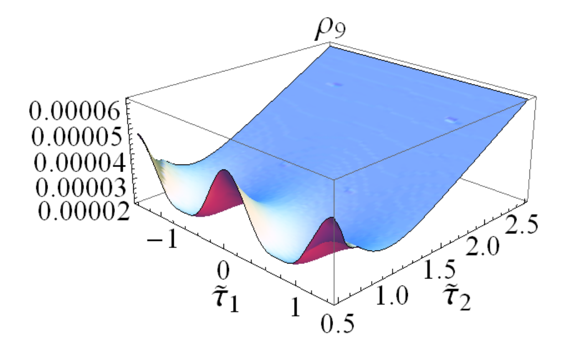
Figure 6: Contour and 3D plots are shown in the left and right panels, respectively, for the energy density ρ9\rho_{9} in the Jordan frame as a function of τ~1=r​A/α′\tilde{\tau}_{1}=rA/\sqrt{\alpha^{\prime}} and τ~2=r/α′\tilde{\tau}_{2}=r/\sqrt{\alpha^{\prime}}, with all their values being given in α′=1\alpha^{\prime}=1 units. In the left, we shade the fundamental region for the T-dual transformation: |τ1|≤1/2\left|\tau_{1}\right|\leq 1/\sqrt{2}, |τ|≥1\left|\tau\right|\geq 1. We can see the shift-symmetry τ~1→τ~1+2\tilde{\tau}_{1}\to\tilde{\tau}_{1}+\sqrt{2}, up to distortions due to numerical errors.

For varying AA and rr, we plot ρ9\rho_{9} as a function of τ~1=r​A/α′\tilde{\tau}_{1}=rA/\sqrt{\alpha^{\prime}} and τ~2=r/α′\tilde{\tau}_{2}=r/\sqrt{\alpha^{\prime}} in Fig. 6. Note that in the large rr (=α′​τ~2=\sqrt{\alpha^{\prime}}\tilde{\tau}_{2}) limit, the Jordan frame potential becomes proportional to rr. This can also be seen analytically from the fact that in the large rr limit, the contributing modes are as in Eq. (56), which results in the same expression as Eq. (16). To repeat, we have obtained both numerically and analytically that the Jordan frame potential is proportional to rr at the one-loop level. For large rr limit, all the higher loop corrections have the same behavior since it comes from the fact that the energy is proportional to the volume of the compactified dimension.

Refer to caption
Refer to caption

Figure 7: Contour and 3D plots are shown in the left and right panels, respectively, for the energy density VEV_{\text{E}} in the Einstein frame as a function of τ~1=r​A/α′\tilde{\tau}_{1}=rA/\sqrt{\alpha^{\prime}} and τ~2=r/α′\tilde{\tau}_{2}=r/\sqrt{\alpha^{\prime}}, with all their values being given in α′=1\alpha^{\prime}=1 units. The shaded fundamental region and the existence of the 2\sqrt{2}-shift are the same as in Fig. 6. We see that the potential becomes runaway for the large radius limit r≫α′r\gg\sqrt{\alpha^{\prime}}.

Now let us turn to the Einstein frame:

VE​(r)\displaystyle V_{E}(r) =−1(2​π​r)2/7​ZT22​π​r​V9,\displaystyle=-{1\over\left({2\pi r}\right)^{2/7}}{Z_{T^{2}}\over 2\pi rV_{9}},
=−1α′9/212​(2​π)72/71r9/7∫Fd​τ1​d​τ2τ211/21|η⁡(τ)|16​η​(τ)16​η¯​(τ¯)4∑sector α​w→Z~T2,α​w→;\displaystyle=-{1\over\alpha^{\prime 9/2}}{1\over 2\left(2\pi\right)^{72/7}}{1\over r^{9/7}}\int_{F}{d\tau_{1}d\tau_{2}\over\tau_{2}^{11/2}}{1\over\left|\eta(\tau)\right|^{16}{\eta(\tau)}^{16}{\bar{\eta}(\bar{\tau})}^{4}}\sum_{\text{sector $\alpha\vec{w}$}}\tilde{Z}_{T^{2},\alpha\vec{w}}; (69)

see Eq. (19). We plot this potential in Fig. 7. Important fact is that the potential in the Einstein frame becomes runaway for the large radius limit r≫α′r\gg\sqrt{\alpha^{\prime}}. As discussed above, this behavior should not be altered by the higher loop corrections.

Note that this effective potential in the Einstein frame is reliable only for large r≫α′r\gg\sqrt{\alpha^{\prime}} since the treatment in terms of the effective field theory (14) becomes valid only in this limit; furthermore, we can regard rr as the physical radius only in this limit; see also the argument around Eq. (56).

3.4 Large boost limit

We want to examine the behavior of the Higgs potential in the large field limit. However, in this nine dimensional toy model, there are two flat directions at this level, namely, AA and RR. If the Higgs comes from a similar mechanism to the gauge-Higgs unification, the Higgs field should be identified with AA. Therefore, we check the large AA limit for a fixed RR. This limit is nothing but the large boost limit as is easily seen from Eq. (45): η→∞\eta\rightarrow\infty. From Eqs. (46) and (59), the trajectory in the τ~1\tilde{\tau}_{1}-τ~2\tilde{\tau}_{2} plane is given by

τ~1=Rα′​tanh⁡η,\displaystyle\tilde{\tau}_{1}={R\over\sqrt{\alpha^{\prime}}}\tanh\eta,
τ~2=Rα′​1cosh⁡η.\displaystyle\tilde{\tau}_{2}={R\over\sqrt{\alpha^{\prime}}}{1\over\cosh\eta}. (70)

Since τ~12+τ~22=R2/α′\tilde{\tau}_{1}^{2}+\tilde{\tau}_{2}^{2}=R^{2}/\alpha^{\prime}, this path starts from (0,R/α′)\left(0,\,R/\sqrt{\alpha^{\prime}}\right) for η=0\eta=0, and moves on the circle toward (R/α′, 0)\left(R/\sqrt{\alpha^{\prime}},\,0\right) as η→∞\eta\to\infty. The question is what this trajectory is when mapped onto the fundamental region. The large η\eta behavior depends on the value of R/α′R/\sqrt{\alpha^{\prime}}:

  • •

    If R/α′∈2​ℚR/\sqrt{\alpha^{\prime}}\in\sqrt{2}\mathbb{Q}, then τ~2\tilde{\tau}_{2} (=r/α′=r/\sqrt{\alpha^{\prime}}) goes to infinity in the large η\eta limit. This can be seen as follows. Since τ~→R/α′\tilde{\tau}\to R/\sqrt{\alpha^{\prime}} as η→∞\eta\to\infty, let us check to what point R/α′R/\sqrt{\alpha^{\prime}} is mapped in the fundamental region. Let us write R/α′=2​p/qR/\sqrt{\alpha^{\prime}}=\sqrt{2}p/q with p,q∈ℤp,q\in\mathbb{Z}. By an appropriate times of 2\sqrt{2}-shifts (TT-transfomation in (60)), we can always make |p|<|q|\left|p\right|<\left|q\right|. Performing the inversion (SS-transfomation in (60)), and again doing an appropriate times of 2\sqrt{2}-shifts, we can make the numerator pp smaller and smaller; eventually we get p/q→0p/q\to 0. This corresponds to the infinity τ2→∞\tau_{2}\to\infty in the fundamental region.

    This behavior is expected from the discussion of the general momentum boost in Sec. 2.2. In fact, if and only if R/α′∈2​ℚR/\sqrt{\alpha^{\prime}}\in\sqrt{2}\mathbb{Q}, we can have a lattice point on the light cone in the momentum space, that is, there exist n,m,w∈ℤn,m,w\in\mathbb{Z} such that1111 11 This can be proved as follows. First we show that the conditions (71) and (72) can be met for an arbitrary R/α′∈2​ℚR/\sqrt{\alpha^{\prime}}\in\sqrt{2}\mathbb{Q} by an appropriate choice of n,m,wn,m,w. Let us write R/α′=2​qn/qdR/\sqrt{\alpha^{\prime}}=\sqrt{2}q_{n}/q_{d} with qn,qd∈ℤq_{n},q_{d}\in\mathbb{Z}. The condition (72) reads n​qd/qn+2​w​qn/qd=0nq_{d}/q_{n}+2wq_{n}/q_{d}=0. We can choose nn and ww such that n=n′​qnn=n^{\prime}q_{n} and w=w′​qdw=w^{\prime}q_{d} with n′,w′∈ℤn^{\prime},w^{\prime}\in\mathbb{Z}, resulting in the condition n′​qd+2​w′​qn=0n^{\prime}q_{d}+2w^{\prime}q_{n}=0. This can be satisfied by setting w′=qdw^{\prime}=q_{d} and n′=−2​qnn^{\prime}=-2q_{n}. Then the condition (71) reads 0=!m+12​(n′​qd−2​qn​w′)=m+n′​qd0\stackrel{{\scriptstyle!}}{{=}}m+{1\over 2}\left(n^{\prime}q_{d}-2q_{n}w^{\prime}\right)=m+n^{\prime}q_{d}, which can be satisfied by choosing m=−n′​qdm=-n^{\prime}q_{d}. Next we show that if R/α′∉2​ℚR/\sqrt{\alpha^{\prime}}\not{\in}\sqrt{2}\mathbb{Q}, there is no set of n,m,w∈ℤn,m,w\in\mathbb{Z} that satisfies Eqs. (71) and (72). By putting Eq. (72) into Eq. (71), we get the condition m±2​n​α′R=0m\pm\sqrt{2}n{\sqrt{\alpha^{\prime}}\over R}=0. Therefore, it is necessary that R/α′=∓2n/mR/\sqrt{\alpha^{\prime}}=\mp\sqrt{2}n/m with n,m∈ℤn,m\in\mathbb{Z}.

    lL2−pR2\displaystyle l_{L}^{2}-p_{R}^{2} =2α′​[m+12​(nR/α′−Rα′​w)]​[m−12​(nR/α′−Rα′​w)]=0,\displaystyle={2\over\alpha^{\prime}}\left[m+{1\over\sqrt{2}}\left({n\over R/\sqrt{\alpha^{\prime}}}-{R\over\sqrt{\alpha^{\prime}}}w\right)\right]\left[m-{1\over\sqrt{2}}\left({n\over R/\sqrt{\alpha^{\prime}}}-{R\over\sqrt{\alpha^{\prime}}}w\right)\right]=0, (71)
    pL2\displaystyle p_{L}^{2} =1α′​(nR/α′+Rα′​w)2=0.\displaystyle={1\over\alpha^{\prime}}\left({n\over R/\sqrt{\alpha^{\prime}}}+{R\over\sqrt{\alpha^{\prime}}}w\right)^{2}=0. (72)

    For R/α′∈2​ℚR/\sqrt{\alpha^{\prime}}\in\sqrt{2}\mathbb{Q}, there is a point on the light cone in the momentum space. Following the argument of Sec. 2.2, the Lorentz boost between lLl_{L} and pRp_{R} opens up a new dimension.

  • •

    If R/α′∉2​ℚR/\sqrt{\alpha^{\prime}}\not{\in}\sqrt{2}\mathbb{Q}, the potential becomes either periodic or chaotic. Let us check in what case we get the periodic potential.

    • –

      The periodic case is realized if, starting from a point τ~\tilde{\tau} (70) with the boost η\eta, we get another point on the trajectory with the boost η+ηc\eta+\eta_{c},

      τ~1′\displaystyle\tilde{\tau}_{1}^{\prime} =Rα′​tanh⁡(η+ηc),\displaystyle={R\over\sqrt{\alpha^{\prime}}}\tanh\!\left(\eta+\eta_{c}\right),
      τ~2′\displaystyle\tilde{\tau}_{2}^{\prime} =Rα′​1cosh⁡(η+ηc),\displaystyle={R\over\sqrt{\alpha^{\prime}}}{1\over\cosh\!\left(\eta+\eta_{c}\right)}, (73)

      which can be mapped from τ~\tilde{\tau} by an appropriate T-dual transformation (61).

      In general, the transformation of τ~2\tilde{\tau}_{2} is as shown in Eq. (168), and we get

      τ~2′\displaystyle\tilde{\tau}_{2}^{\prime} =τ~2|c​τ~+d|2=τ~2c2​R2α′+d2+2​c​d​τ~1=Rα′​1(c2​R2α′+d2)​cosh⁡η+2​c​d​Rα′​sinh⁡η\displaystyle={\tilde{\tau}_{2}\over\left|c\tilde{\tau}+d\right|^{2}}={\tilde{\tau}_{2}\over c^{2}{R^{2}\over\alpha^{\prime}}+d^{2}+2cd\tilde{\tau}_{1}}={R\over\sqrt{\alpha^{\prime}}}{1\over\left(c^{2}{R^{2}\over\alpha^{\prime}}+d^{2}\right)\cosh\eta+2cd{R\over\sqrt{\alpha^{\prime}}}\sinh\eta}
      =Rα′​1cosh⁡(η−η2),\displaystyle={R\over\sqrt{\alpha^{\prime}}}{1\over\cosh\!\left(\eta-\eta_{2}\right)}, (74)

      where we have defined η2\eta_{2} by

      tanh⁡η2:=−2​c​d​Rα′c2​R2α′+d2.\displaystyle\tanh\eta_{2}:=-{2cd{R\over\sqrt{\alpha^{\prime}}}\over c^{2}{R^{2}\over\alpha^{\prime}}+d^{2}}. (75)

      On the other hand, the same transformation maps τ~1\tilde{\tau}_{1} to

      τ~1′\displaystyle\tilde{\tau}_{1}^{\prime} =a​c​|τ~|2+(a​d+b​c)​τ~1+b​d|c​τ~+d|2=a​c​R2α′+b​d+(a​d+b​c)​τ1cosh⁡(η−η2)/cosh⁡η\displaystyle={ac\left|\tilde{\tau}\right|^{2}+\left(ad+bc\right)\tilde{\tau}_{1}+bd\over\left|c\tilde{\tau}+d\right|^{2}}={ac{R^{2}\over\alpha^{\prime}}+bd+\left(ad+bc\right)\tau_{1}\over\cosh\!\left(\eta-\eta_{2}\right)/\cosh\eta}
      =(a​c​R2α′+b​d)​cosh⁡η+Rα′​(a​d+b​c)​sinh⁡ηcosh⁡(η−η2)\displaystyle={\left(ac{R^{2}\over\alpha^{\prime}}+bd\right)\cosh\eta+{R\over\sqrt{\alpha^{\prime}}}\left(ad+bc\right)\sinh\eta\over\cosh\!\left(\eta-\eta_{2}\right)}
      =Rα′​sinh⁡(η−η1)cosh⁡(η−η2),\displaystyle={R\over\sqrt{\alpha^{\prime}}}{\sinh\!\left(\eta-\eta_{1}\right)\over\cosh\!\left(\eta-\eta_{2}\right)}, (76)

      where we have defined η1\eta_{1} by

      tanh⁡η1=−a​c​R2α′+b​dRα′​(a​d+b​c).\displaystyle\tanh\eta_{1}=-{ac{R^{2}\over\alpha^{\prime}}+bd\over{R\over\sqrt{\alpha^{\prime}}}\left(ad+bc\right)}. (77)

      The trajectory becomes periodic if and only if η1=η2\eta_{1}=\eta_{2}, that is,

      2​c​d​Rα′c2​R2α′+d2\displaystyle{2cd{R\over\sqrt{\alpha^{\prime}}}\over c^{2}{R^{2}\over\alpha^{\prime}}+d^{2}} =a​c​R2α′+b​dRα′​(a​d+b​c),\displaystyle={ac{R^{2}\over\alpha^{\prime}}+bd\over{R\over\sqrt{\alpha^{\prime}}}\left(ad+bc\right)}, (78)

      or

      (d2−c2​R2α′)​(b​d−a​c​R2α′)\displaystyle\left(d^{2}-c^{2}{R^{2}\over\alpha^{\prime}}\right)\left(bd-ac{R^{2}\over\alpha^{\prime}}\right) =0.\displaystyle=0. (79)

      Vanishing first factor means η2=∞\eta_{2}=\infty, and the finite period is obtained when and only when the last factor becomes zero:

      b​d−a​c​R2α′\displaystyle bd-ac{R^{2}\over\alpha^{\prime}} =0.\displaystyle=0. (80)

      Therefore, the partition function becomes periodic if and only if R2/α′R^{2}/\alpha^{\prime} can be written as

      R2​α′∉ℚ,\displaystyle{R\over\sqrt{2\alpha^{\prime}}}\not{\in}\mathbb{Q}, R2α′=b​da​c,\displaystyle{R^{2}\over\alpha^{\prime}}={bd\over ac}, (81)

      where a​d−b​c=1ad-bc=1 and either a,d∈2​ℤa,d\in\sqrt{2}\mathbb{Z}, b,c∈ℤb,c\in\mathbb{Z} or a,d∈ℤa,d\in\mathbb{Z}, b,c∈2​ℤb,c\in\sqrt{2}\mathbb{Z}.

    • –

      In particular, if R2/α′R^{2}/\alpha^{\prime} is an irrational number then the condition (81) cannot be met (unless a​c=0ac=0 that leads to the trivial η1=0\eta_{1}=0), and the partition function becomes non-periodic, namely chaotic.

Refer to caption
Refer to caption
Refer to caption

Figure 8: The trajectory that starts from η=0\eta=0 at (τ~1,τ~2)=(0,R/α′)\left(\tilde{\tau}_{1},\tilde{\tau}_{2}\right)=\left(0,R/\sqrt{\alpha^{\prime}}\right) for a fixed value of R/α′R/\sqrt{\alpha^{\prime}} being 2\sqrt{2}, 2, and 21/32^{1/3} in the left, center, and right panels, respectively, showing the runaway, periodic, and chaotic limits. We have shaded the fundamental region for the T-dual transformations.

As a check, we show the numerical results for R/α′=2R/\sqrt{\alpha^{\prime}}=\sqrt{2}, 22, and 21/32^{1/3} in Fig. 8. We see that they show the runaway, periodic, and chaotic limits, respectively. The result presented in this section provides a concrete example of the general argument presented in Sec. 2. It is plausible that the large Higgs field limit in string theory fits into either one of these three.

Note that our computation is based on the one-loop effective potential and that the higher order corrections are significant around the region A,R−1∼MsA,R^{-1}\sim M_{\text{s}} (=1/α′=1/\sqrt{\alpha^{\prime}}). Therefore, the result so far should be interpreted as an effort to guess what is the physical large field limit along a potential valley after including all the higher order corrections. In Fig. 8, we have checked the large AA limit for a fixed RR. Is this a physical limit, and if not, what should it be? Comparing Figs. 6 and 7, we see that it is a generic feature that there is a runaway vacuum no matter what the structure is around A,R−1∼MsA,R^{-1}\sim M_{\text{s}}. It seems plausible that if the physical large AA limit is not the one with fixed τ~2\tilde{\tau}_{2}, then large AA limit goes into the runaway vacuum after all. However, we consider all the three limits, runaway, periodic, and chaotic in order not to loose generality.

Refer to caption

Figure 9: Schematic figure for the Higgs potential. Low energy side is determined phenomenologically. High energy side represents a runaway direction in the multi degrees of freedom space.

As said above, the extrapolation from the low energy data has revealed that there is the quasi-flat direction of the Higgs potential in the SM. We are interested in the potential for the large field values. Beyond the string or Planck scale, there opens up several quasi-flat directions in general. Therefore we need to consider a multi-dimensional field space. In the example examined in this section, it corresponds to the AA-RR (or τ~1\tilde{\tau}_{1}-τ~2\tilde{\tau}_{2}) plane. As we have seen in this section, generally there is at least one runaway direction in this space that corresponds to opening up an extra dimension; see Fig. 9. We will discuss its physical implications in the subsequent sections.

4 Eternal Higgs inflation

As shown in Introduction, the Higgs potential V∼λeff​|H|4V\sim\lambda_{\text{eff}}\left|H\right|^{4} in the SM shows a quite peculiar behavior when extrapolated to very large field values: all of the λeff\lambda_{\text{eff}}, its running, and the bare Higgs mass can be accidentally small. In Ref. [61], we have proposed a possibility that this behavior, so to say the criticality, is a consequence of the Planck scale physics and that the criticality is closely related to the cosmic inflation.

Refer to caption

Figure 10: Schematic figure for the maximum that yields the domain wall, which becomes the source for the eternal inflation.

We have seen that the large field limit goes down to a runaway direction, which corresponds to opening up an extra dimension, in the multi degrees of freedom space, as shown in Fig. 9. Therefore, there is at least one maximum of the potential around the Planck scale; see Fig. 10. This maximum can be a source of an eternal inflation at the core of the domain wall [105] between the electroweak vacuum and the runaway vacuum, in which the fifth dimension is opened up. In order for this to work, the curvature of the potential at the maximum must be sufficiently small [106]:

MP2​Vφ​φV|maximum≲1.4.\displaystyle\left.M_{P}^{2}{V_{\varphi\varphi}\over V}\right|_{\text{maximum}}\lesssim 1.4. (82)

In our scenario, this can be naturally satisfied as follows. The potential for the fifth dimension can be seen by putting D=5D=5 in Eq. (19). In stringy language, the action for the fifth dimension R′≫Ms−1R^{\prime}\gg M_{\text{s}}^{-1} is coming from the one-loop potential: In the Einstein frame, we get

Seff\displaystyle S_{\text{eff}} ∼Ms2gs2​∫d4​x​−g​(ℛ−(∂R′)2R′2−gs2​Ms2​1R′).\displaystyle\sim{M_{\text{s}}^{2}\over g_{\text{s}}^{2}}\int\text{d}^{4}x\sqrt{-g}\left(\mathcal{R}-{\left(\partial R^{\prime}\right)^{2}\over R^{\prime 2}}-g_{\text{s}}^{2}M_{\text{s}}^{2}{1\over R^{\prime}}\right). (83)

Switching to the canonical field R′=egs​χ/MsR^{\prime}=e^{g_{\text{s}}\chi/M_{\text{s}}}, we get

Seff\displaystyle S_{\text{eff}} ∼∫d4x−g(MP2ℛ−(∂χ)2−e−χ/MPMs4),\displaystyle\sim\int\text{d}^{4}x\sqrt{-g}\left(M_{\text{P}}^{2}\mathcal{R}-\left(\partial\chi\right)^{2}-e^{-\chi/M_{\text{P}}}M_{\text{s}}^{4}\right), (84)

where MP=Ms/gsM_{\text{P}}=M_{\text{s}}/g_{\text{s}}. Therefore, the stringy potential also gives

Vχ​χ\displaystyle V_{\chi\chi} ∼VMP2.\displaystyle\sim{V\over M_{\text{P}}^{2}}. (85)

It is remarkable that the potential changes of order unity when we vary χ\chi by MPM_{\text{P}}, not by MsM_{\text{s}}, for large χ\chi. On the other hand at low energies, the SM potential in the Einstein frame exhibits the same behavior if the non-minimal coupling ξ\xi is of order ten [65]. Therefore, it is natural to conclude that the condition (82) is also met around the maximum.

We note that in the original version of the topological Higgs inflation [105], ξ\xi is used to make the maximum of the potential, and hence that it cannot account for the observed fluctuation of the cosmic microwave background (CMB). On the other hand, the scenario proposed in this paper allows the Higgs to be the source for both the eternal topological inflation and for the one that accounts for the CMB fluctuation, simultaneously.

Refer to caption

Figure 11: Schematic figure for the Higgs potential smoothly connected to the runaway direction.
Refer to caption
Refer to caption

Figure 12: Schematic figure for the Higgs potential. On the left, the false vacuum has higher energy than the quasi-flat potential in the SM, while on the right, it has lower energy.

There are two possibilities for the potential beyond the maximum:

  • •

    The potential smoothly becomes runaway as in Fig. 11.

  • •

    The potential has another local minimum as in Fig. 12.

In the latter case, the false vacuum gives another mechanism of eternal inflation. This situation is similar to some of the originators’ idea of the inflation using a first order phase transition [107, 108]. In the medium of the false vacuum, which is indicated by the (red) dot in Fig. 12, there appears a bubble of the electroweak vacuum due to the tunneling, which is indicated by the dotted arrow. This eternal inflation in the false vacuum had caused the so-called the graceful exit problem in the old inflation scenario [109, 110, 111]. However in the left case in Fig. 12, the space inside the bubble experiences the second stage of inflation [61, 65], after the dotted arrow in the figure, and hence this problem is ameliorated as we do not need bubbles to collide. In the right case in Fig. 12, we need another inflation to account for the observed CMB fluctuation such as the B−LB-L Higgs inflation.

5 Cosmological constant

As is reviewed in detail in Appendix D, the MPP requires degenerate vacua at the field value of the order of the Planck scale [36, 37, 38]. The cosmological constant of the runaway vacuum is exactly zero. Then the MPP tells us that our electroweak vacuum must have the zero cosmological constant too. This is a new solution to the cosmological constant problem in terms of the MPP.1212 12 See also Ref. [38] in which the cosmological constant problem is discussed in a different perspective.

On the other hand, the current universe is being dominated by the cosmological constant [112]

ρΛobs≃(2.2​meV)4,\displaystyle\rho_{\Lambda}^{\text{obs}}\simeq\left(2.2\,\text{meV}\right)^{4}, (86)

and is entering the second inflationary stage. This will eventually lead to the de Sitter space d​S4dS_{4} with the length scale H−1H^{-1}, where

H2=ρΛobs3​MP2.\displaystyle H^{2}={\rho_{\Lambda}^{\text{obs}}\over 3M_{P}^{2}}. (87)

We will discuss the possibility that the existence of the finite cosmological constant is understood as a statistical fluctuation.

Refer to caption

Figure 13: Universe is divided into parts that will eventually become causally disconnected to each other in the end of their histories.

First we point out that our universe is a part of a large universe whose cosmological constant is fixed to zero by the MPP.1313 13 The argument in this section may also apply for the multiverse [54, 55, 56, 57, 58]. The large universe can be divided into parts that will eventually become causally disconnected de Sitter spaces in the end of their histories, as in Fig. 13. After the Euclideanization, each de Sitter space becomes S4S^{4} with radius rU=1/Hr_{U}=1/H.

We consider one of the S4S^{4}’s and latticize it by the lattice spacing of the order of łP=1/MP\l_{P}=1/M_{\text{P}}, and let SiS_{i} be the action on each site labeled by ii. The total action for the S4S^{4} becomes the sum over positions:

S\displaystyle S =∑i=1rU4/lP4Si.\displaystyle=\sum_{i=1}^{r_{U}^{4}/l_{P}^{4}}S_{i}. (88)

Assuming that SiS_{i} are independent of each other, the vanishing cosmological constant for the large universe leads to ⟨Si⟩=0\Braket{S_{i}}=0 for each ii and in particular to ⟨S⟩=0\Braket{S}=0 for this part. Therefore the value of SS fluctuates around zero and its variance can be evaluated as

⟨S2⟩∼N:=rU4lP4,\displaystyle\Braket{S^{2}}\sim N:={r_{U}^{4}\over l_{P}^{4}}, (89)

where we have assumed that the variance of each SiS_{i} is of order unity.

We interpret Eq. (89) as the variance of the actions of the S4S^{4}’s in the large universe. Then the typical amount of the energy density of one S4S^{4} is estimated as

ρΛ∼⟨S2⟩rU4∼1lP2​rU2∼(meV)4.\displaystyle\rho_{\Lambda}\sim{\sqrt{\Braket{S^{2}}}\over r_{U}^{4}}\sim{1\over l_{P}^{2}r_{U}^{2}}\sim\left(\,\text{meV}\right)^{4}. (90)

Thus, we have obtained the right amount of the cosmological constant as the fluctuation from zero. This result has been obtained in Ref. [113] in the context of causal set theory.

We note that the value of HH is not really a prediction in this argument. We have rather provided a consistent explanation of having a finite amount of the cosmological constant, even though it is fixed to be zero for the large universe.

6 Summary and discussions

We have studied possible large field limits of the SM Higgs, assuming that it is coming from a massless state at the tree level in heterotic string theory with its supersymmetry broken at the string scale. In the toroidal compactification, putting a background for such a massless state corresponds to a boost in the momentum lattice. We have classified the large boost limits with fixed radius into three categories: runaway, periodic, and chaotic.

As a concrete toy model, we have examined the ten-dimensional S​O​(16)×S​O​(16)SO(16)\times SO(16) non-supersymmetric heterotic string, with a dimension being compactified on S1S^{1} with the radius RR. We have considered the large field limit of a Wilson line on the S1S^{1} with fixed RR, and reproduced these three limits. We have argued that this behavior is universal if the zero momentum limit of the emission vertex of the Higgs is written as a product of holomorphic (1,0) and anti-holomorphic (0,1) operators, not only in the case of toroidal compactification. In the known models of fermionic construction and of orbifolding, the emission vertex tends to be written as such a product, and our argument applies for these wide class of models.

Physically several degrees of freedom appears when the Higgs field value becomes larger than the Planck scale. We have argued that there exists an runaway direction in this multi degrees of freedom space. This runaway vacuum corresponds to opening up an extra dimension.

It is noteworthy that this potential fits into the criteria of the MPP proposed by Froggatt and Nielsen. The MPP requires that the electroweak vacuum is degenerate with this runaway vacuum, and hence that the cosmological constant of the electroweak vacuum is tuned to be zero in the large universe. We have speculated that the observed amount of the cosmological constant can be understood as a fluctuation from zero in the framework of the MPP.

We may get the eternal inflation from this potential. It is realized either as a topological inflation at the domain wall between the two vacua or as a decay from the false vacuum that traps the Higgs field. In both cases, the Higgs field, which is rolling down the potential, may cause the succeeding inflation, which accounts for the observed CMB fluctuations, along the quasi-flat potential around the critical point.

It would be interesting to study the limit in more realistic SM-like model with the orbifolding, fermionic constructions, etc; see e.g. Ref. [73].

Finally we comment on the dilaton potential. Though we consider the general compactifications which may not even have a geometric interpretation, let us illustrate the situation starting from a conventional ten dimensional string theory. The low energy effective action in ten dimensions reads

S\displaystyle S =Ms8gs2​∫d10​x​−g​e−2​Φ​(ℛ+4​∂μΦ​∂μΦ+⋯)\displaystyle={M_{\text{s}}^{8}\over g_{\text{s}}^{2}}\int\text{d}^{10}x\sqrt{-g}\,e^{-2\Phi}\left(\mathcal{R}+4\partial_{\mu}\Phi\,\partial^{\mu}\Phi+\cdots\right)
+Ms10∫d10x−g(−C+⋯)\displaystyle\quad+M_{\text{s}}^{10}\int\text{d}^{10}x\sqrt{-g}\left(-C+\cdots\right)
+𝒪⁡(gs2​e2​Φ),\displaystyle\quad+\mathcal{O}\!\left(g_{s}^{2}e^{2\Phi}\right), (91)

where Φ\Phi is the dilaton field and CC is the dimensionless cosmological constant induced at the one-loop level. We note that in this string frame, gsg_{\text{s}} and Φ\Phi always appear in the combination gs​eΦg_{\text{s}}e^{\Phi}. After the compactification,

S\displaystyle S =Ms2gs2​(Ms6​V6)​∫d4​x​−g4​e−2​Φ​(ℛ4+4​∂μΦ​∂μΦ+⋯)\displaystyle={M_{\text{s}}^{2}\over g_{\text{s}}^{2}}\left(M_{\text{s}}^{6}V_{6}\right)\int\text{d}^{4}x\sqrt{-g_{4}}\,e^{-2\Phi}\left(\mathcal{R}_{4}+4\partial_{\mu}\Phi\,\partial^{\mu}\Phi+\cdots\right)
+Ms4(Ms6V6)∫d4x−g4(−C+⋯)\displaystyle\quad+M_{\text{s}}^{4}\left(M_{\text{s}}^{6}V_{6}\right)\int\text{d}^{4}x\sqrt{-g_{4}}\left(-C+\cdots\right)
+𝒪⁡(gs2​e2​Φ),\displaystyle\quad+\mathcal{O}\!\left(g_{s}^{2}e^{2\Phi}\right), (92)

where V6V_{6} is the compactification volume. Switching to the Einstein frame, we get

S\displaystyle S =Ms2gs2​(Ms6​V6)​∫d4​x​−gE​(ℛE−2​∂μΦ​∂μΦ+⋯)\displaystyle={M_{\text{s}}^{2}\over g_{\text{s}}^{2}}\left(M_{\text{s}}^{6}V_{6}\right)\int\text{d}^{4}x\sqrt{-g_{E}}\left(\mathcal{R}_{E}-2\partial_{\mu}\Phi\,\partial^{\mu}\Phi+\cdots\right)
+Ms4(Ms6V6)∫d4x−gE(−Ce4​Φ+⋯)\displaystyle\quad+M_{\text{s}}^{4}\left(M_{\text{s}}^{6}V_{6}\right)\int\text{d}^{4}x\sqrt{-g_{E}}\left(-C\,e^{4\Phi}+\cdots\right)
+⋯.\displaystyle\quad+\cdots. (93)

We see from the second line that the dilaton has the runaway potential e4​Φe^{4\Phi} for Φ→−∞\Phi\to-\infty if the cosmological constant CC is positive. In this limit, the expansion parameter gs​eΦg_{s}e^{\Phi} in Eq. (92) becomes small, and the theory is weakly coupled. Since all the higher-loop corrections come with this combination as well, the runaway behavior is not altered by taking them into account. Therefore, this direction Φ→−∞\Phi\to-\infty necessarily comprises one of the runaway directions [78] in Fig. 9, and hence the arguments in Sections 4 and 5 apply quite generally.

Acknowledgement

We thank Michael Blaszczyk, Stefan Groot Nibbelink, Orestis Loukas, Sául Ramos-Sánchez, and Toshifumi Yamashita for useful comments. This work is in part supported by the Grant-in-Aid for Scientific Research Nos. 22540277 (HK), 23104009, 20244028, and 23740192 (KO). The work of Y. H. is supported by a Grant-in-Aid for Japan Society for the Promotion of Science (JSPS) Fellows No.25⋅\cdot1107.

Appendix A Theta functions

We list the notations for the functions that we use in the computation of the partition function. (The notations are the same as in Polchinski’s textbook but we list them anyway for convenience.) The Dedekind eta function is

η⁡(τ)=q1/24​∏n=1∞(1−qn),\displaystyle\eta(\tau)=q^{1/24}\prod_{n=1}^{\infty}\left(1-q^{n}\right), (94)

where q=e2​π​τq=e^{2\pi\tau}. We write theta function with characteristics as

ϑ​[ab]​(ν,τ)\displaystyle\vartheta\begin{bmatrix}a\\ b\end{bmatrix}(\nu,\tau) =∑n=−∞∞exp⁡(π​i​(n+a)2​τ+2​π​i​(n+a)​(ν+b)),\displaystyle=\sum_{n=-\infty}^{\infty}\exp\!\left(\pi i\left(n+a\right)^{2}\tau+2\pi i\left(n+a\right)\left(\nu+b\right)\right), (95)

and introduce the following shorthand notations:

ϑ00​(τ)\displaystyle\vartheta_{00}(\tau) =ϑ​[00]​(0,τ),\displaystyle=\vartheta\begin{bmatrix}0\\ 0\end{bmatrix}(0,\tau), (96)
ϑ01​(τ)\displaystyle\vartheta_{01}(\tau) =ϑ​[01/2]​(0,τ),\displaystyle=\vartheta\begin{bmatrix}0\\ 1/2\end{bmatrix}(0,\tau), (97)
ϑ10​(τ)\displaystyle\vartheta_{10}(\tau) =ϑ​[1/20]​(0,τ),\displaystyle=\vartheta\begin{bmatrix}1/2\\ 0\end{bmatrix}(0,\tau), (98)
ϑ11​(τ)\displaystyle\vartheta_{11}(\tau) =ϑ​[1/21/2]​(0,τ)=0.\displaystyle=\vartheta\begin{bmatrix}1/2\\ 1/2\end{bmatrix}(0,\tau)=0. (99)

The Jacobi’s identity reads

(ϑ00)4−(ϑ01)4−(ϑ10)4=0.\displaystyle\left(\vartheta_{00}\right)^{4}-\left(\vartheta_{01}\right)^{4}-\left(\vartheta_{10}\right)^{4}=0. (100)

Appendix B Fermionic construction manual for ten dimensions

We review the S​O​(16)×S​O​(16)SO(16)\times SO(16) heterotic string theory in terms of the fermionic construction, and show the computation of its one-loop partition function. In heterotic string theory, the right-moving modes are the same as the superstring in 10 dimensions XμX^{\mu} (μ=0,…,9\mu=0,\dots,9), while the left-movers as the bosonic string in 26 dimensions with their “internal” XLIX_{L}^{I} (I=1,…,16I=1,\dots,16) being compactified.

B.1 Generalized GSO projection

We work in the light-cone gauge, where X+X^{+} is identified with the time direction and X−X^{-} is written in terms of the transverse modes, where

X±=12​(X0±X1).\displaystyle X_{\pm}={1\over\sqrt{2}}(X^{0}\pm X^{1}). (101)

We express the left-moving extra degrees of freedom XLIX_{L}^{I} by 16 complex fermions, while we form 4 complex fermions by pairing the right-moving fermions ψRm\psi_{R}^{m} (m=2,…,9m=2,\dots,9). Hereafter, ψa\psi^{a} (a=1,…,4a=1,\dots,4) denote the 4 complex fermions representing ψRm\psi_{R}^{m}, and ψa\psi^{a} (a=5,…,20a=5,\dots,20) denote the 16 complex fermions representing XLIX_{L}^{I}.

Refer to caption

Figure 14: A and P denote the anti-periodic and periodic boundary conditions, respectively. The horizontal direction is the spatial one, σ\sigma. Given the all-A boundary condition for both the time and spatial directions, the modular invariance necessitates the all-P boundary condition for the time or spatial direction.
Refer to caption

Figure 15: Schematic picture for the string interaction joining w→i\vec{w}_{i} and w→j\vec{w}_{j} strings to make w→i+w→j\vec{w}_{i}+\vec{w}_{j} string. If there exist the sets of boundary conditions w→i\vec{w}_{i} and w→j\vec{w}_{j}, then there must be w→i+w→j\vec{w}_{i}+\vec{w}_{j} in WW.

Let us review the procedure to retain the modular invariance. Here we assume that each of the above-listed complex fermions ψa\psi^{a} (a=1,…,20a=1,\dots,20) either has the NS (anti-periodic) or R (periodic) boundary condition on the worldsheet σ∼σ+2​π\sigma\sim\sigma+2\pi:1414 14 One can consider a more general boundary condition such as ψa​(σ=2​π)=±ψa¯​(σ=0)\psi^{a}\!\left(\sigma=2\pi\right)=\pm\overline{\psi^{a}}\!\left(\sigma=0\right) and ψa​(σ=2​π)=−e2​π​i​wa​ψa​(σ=0)\psi^{a}\!\left(\sigma=2\pi\right)=-e^{2\pi iw_{a}}\psi^{a}\!\left(\sigma=0\right) for arbitrary rational waw^{a} [104].

NS: ψa(σ=2π)\displaystyle\text{NS: }\quad\psi^{a}\!\left(\sigma=2\pi\right) =−ψa​(σ=0),\displaystyle=-\psi^{a}\!\left(\sigma=0\right),
R: ψa(σ=2π)\displaystyle\text{R: }\quad\psi^{a}\!\left(\sigma=2\pi\right) =ψa​(σ=0).\displaystyle=\psi^{a}\!\left(\sigma=0\right). (102)

We can write them collectively

ψa​(σ=2​π)\displaystyle\psi^{a}\!\left(\sigma=2\pi\right) =−e2​π​i​wa​ψa​(σ=0),\displaystyle=-e^{2\pi iw^{a}}\psi^{a}\!\left(\sigma=0\right), (103)

where the vector w→=(wa)a=1,…,20\vec{w}=\left(w^{a}\right)_{a=1,\dots,20} consists of either 0 (NS, anti-periodic) or 1/21/2 (R, periodic) modulo 1.

We classify the possible boundary conditions by the following procedure. Let WW be a vector space over Z2Z_{2} spanned by the bases {w→i}i=0,…,l\Set{\vec{w}_{i}}_{i=0,\dots,l}. WW is the set of boundary conditions, appearing in a theory, that are required by the string interaction and the modular invariance:

  • •

    There must be all anti-periodic boundary condition

    0→=(0)a=1,…,20=(0,…,0)\displaystyle\vec{0}=\left(0\right)_{a=1,\dots,20}=\left(0,\dots,0\right) (104)

    in WW: When considering a partition function on the torus, there must be the sector in which all the fermions are anti-periodic in the time direction in order to get the identity operator in the trace, which is needed to form a projection operator; then the SS-transformation τ→−1/τ\tau\to-1/\tau maps this condition to the space direction.

  • •

    Then the modular invariance necessitates the all-periodic boundary condition

    w→0:=(1/2)a=1,…,20=(1/2,…,1/2)\displaystyle\vec{w}_{0}:=\left(1/2\right)_{a=1,\dots,20}=\left(1/2,\dots,1/2\right) (105)

    in WW; see Fig. 14.

  • •

    If w→i\vec{w}_{i} and w→j\vec{w}_{j} exist in WW, then w→i+w→j\vec{w}_{i}+\vec{w}_{j} must also be in WW; see Fig. 15.

A boundary condition belonging to WW can be written as

ψa​(σ=2​π)\displaystyle\psi^{a}\!\left(\sigma=2\pi\right) =−e2​π​i​(α​w→)a​ψa​(σ=0),\displaystyle=-e^{2\pi i\left(\alpha\vec{w}\right)^{a}}\psi^{a}\!\left(\sigma=0\right), (106)

where α​w→:=∑i=0lαi​w→i\alpha\vec{w}:=\sum_{i=0}^{l}\alpha_{i}\vec{w}_{i}, namely (α​w→)a:=∑i=0lαi​wia\left(\alpha\vec{w}\right)^{a}:=\sum_{i=0}^{l}\alpha_{i}w_{i}^{a}, with αi\alpha_{i} (i=0,…,li=0,\dots,l) being either 0 or 1 and the vector w→i=(wia)a=1,…,20\vec{w}_{i}=\left(w_{i}^{a}\right)_{a=1,\dots,20} consisting of either 0 or 1/21/2 again.

The partition function becomes modular invariant if and only if we impose the generalized GSO projection, under which the surviving states satisfy the following condition [104]:

e2​π​i​w→i⋅N→α​w→\displaystyle e^{2\pi i\vec{w}_{i}\cdot\vec{N}_{\alpha\vec{w}}} =e2​π​i​(∑j=0lki​j​αj−w→i⋅α​w→¯¯+si),for each i=0,…,l,\displaystyle=e^{2\pi i\left(\sum_{j=0}^{l}k_{ij}\alpha_{j}-\vec{w}_{i}\cdot\overline{\overline{\alpha\vec{w}}}+s_{i}\right)},\qquad\text{for each $i=0,\dots,l$,} (107)

that is,

w→i⋅N→α​w→\displaystyle\vec{w}_{i}\cdot\vec{N}_{\alpha\vec{w}} =1∑j=0lki​j​αj−w→i⋅α​w→¯¯+si,for each i=0,…,l,\displaystyle\stackrel{{\scriptstyle 1}}{{=}}\sum_{j=0}^{l}k_{ij}\alpha_{j}-\vec{w}_{i}\cdot\overline{\overline{\alpha\vec{w}}}+s_{i},\qquad\text{for each $i=0,\dots,l$,} (108)

where =1\stackrel{{\scriptstyle 1}}{{=}} stands for the equality modulo 1; N→α​w→\vec{N}_{\alpha\vec{w}} is the vector consisting of the worldsheet fermion numbers for the α​w→\alpha\vec{w} sector; the inner product is Lorentzian such that ++ and −- are respectively assigned for right and left movers,

w→i⋅w→j\displaystyle\vec{w}_{i}\cdot\vec{w}_{j} :=∑a=14wia​wja−∑b=520wib​wjb;\displaystyle:=\sum_{a=1}^{4}{w}_{i}^{a}{w}_{j}^{a}-\sum_{b=5}^{20}{w}_{i}^{b}{w}_{j}^{b}; (109)

sis_{i} denotes the value of the right-moving components of wiaw_{i}^{a} (a=1,…,4a=1,\dots,4),

si:=wi1=wi2=wi3=wi4\displaystyle s_{i}:=w_{i}^{1}=w_{i}^{2}=w_{i}^{3}=w_{i}^{4} (110)

(∑i=0lαi​si=0\sum_{i=0}^{l}\alpha_{i}s_{i}=0 and 1/21/2 respectively indicate that the α​w→\alpha\vec{w} sector is a spacetime boson and fermion);1515 15 All the right-moving components must take the same value as in Eq. (110) since we assume the 10 dimensional Lorentz invariance. α​w→¯¯\overline{\overline{\alpha\vec{w}}} is the vector, each of its component being the fractional part of the corresponding component of α​w→\alpha\vec{w}, that is, α​w→¯¯\overline{\overline{\alpha\vec{w}}} is the fractional vector in the decomposition1616 16 The fractional vector is chosen in such a way that all its components are within [−1/2,1/2)[-1/2,1/2). In our application, w→i⋅α​w→¯¯\vec{w}_{i}\cdot\overline{\overline{\alpha\vec{w}}} turns out to be zero.

α​w→=∑i=0lαi​w→i=(integer vector)+(fractional vector);\displaystyle\alpha\vec{w}=\sum_{i=0}^{l}\alpha_{i}\vec{w}_{i}=\text{(integer vector)}+\text{(fractional vector)}; (111)

and ki​jk_{ij} is the solution to the following conditions

ki​j+kj​i\displaystyle k_{ij}+k_{ji} =1w→i⋅w→j\displaystyle\stackrel{{\scriptstyle 1}}{{=}}\vec{w}_{i}\cdot\vec{w}_{j}
ki​j​mj\displaystyle k_{ij}m_{j} =10,\displaystyle\stackrel{{\scriptstyle 1}}{{=}}0, all the indices i,j=0,…,li,j=0,\dots,l unsummed,
ki​i+ki​0+si\displaystyle k_{ii}+k_{i0}+s_{i} =112​w→i⋅w→i,\displaystyle\stackrel{{\scriptstyle 1}}{{=}}{1\over 2}\vec{w}_{i}\cdot\vec{w}_{i}, (112)

with mim_{i} being the smallest integer that satisfies mi​w→i=10→m_{i}\vec{w}_{i}\stackrel{{\scriptstyle 1}}{{=}}\vec{0} for each ii unsummed (In our case mi=2m_{i}=2).

For a given WW, the condition (112) may have several solutions for ki​jk_{ij}. Each solution ki​jk_{ij} gives a 10 dimensional string theory that is in general physically distinct from the others. These solutions are believed to complete all the possible consistent string theories in 10 dimensions [104]. To summarize, once a set of basis vectors {w→i}i=0,…,l\Set{\vec{w}_{i}}_{i=0,\dots,l} is given, then one can construct consistent string theories according to the above procedure. A concrete example is shown below.

B.2 E8×E8E_{8}\times E_{8} and S​O​(16)×S​O​(16)SO(16)\times SO(16) string theories

We can obtain the E8×E8E_{8}\times E_{8} superstring theory and the S​O​(16)×S​O​(16)SO(16)\times SO(16) non-supersymmetric string theory by the following choice of basis:1717 17 S​O​(32)SO(32) supersymmetric string corresponds to the bases {w→0,w→1}\Set{\vec{w}_{0},\vec{w}_{1}}.

w→0\displaystyle\vec{w}_{0} =((12)4|(12)8​(12)8),\displaystyle=\left(\left({1\over 2}\right)^{4}\,\bigg|\,\left({1\over 2}\right)^{8}\,\left({1\over 2}\right)^{8}\right),
w→1\displaystyle\vec{w}_{1} =(04|(12)8​(12)8),\displaystyle=\left(0^{4}\,\bigg|\,\left({1\over 2}\right)^{8}\,\left({1\over 2}\right)^{8}\right),
w→2\displaystyle\vec{w}_{2} =(04|(12)8​ 08),\displaystyle=\left(0^{4}\,\bigg|\,\left({1\over 2}\right)^{8}\,0^{8}\right), (113)

where 00 and 1/21/2 represent the anti-periodic and periodic boundary conditions, respectively, as explained above; those on the left (right) of || are the boundary conditions for the right (left) moving fermions; and e.g. 040^{4} denote that there are four 00s in the slots.

Let us obtain ki​jk_{ij} for the basis (113). We express ki​jk_{ij} by a three-by-three matrix:

k=[k00k01k02k10k11k12k20k21k22]=[abcdefghi].\displaystyle k=\begin{bmatrix}k_{00}&k_{01}&k_{02}\\ k_{10}&k_{11}&k_{12}\\ k_{20}&k_{21}&k_{22}\end{bmatrix}=\begin{bmatrix}a&b&c\\ d&e&f\\ g&h&i\end{bmatrix}. (114)

Noting that m0=m1=m2=2m_{0}=m_{1}=m_{2}=2, s0=1/2s_{0}=1/2, s1=s2=0s_{1}=s_{2}=0, w→0⋅w→0=−3\vec{w}_{0}\cdot\vec{w}_{0}=-3, w→1⋅w→1=w→0⋅w→1=−4\vec{w}_{1}\cdot\vec{w}_{1}=\vec{w}_{0}\cdot\vec{w}_{1}=-4, and w→2⋅w→2=w→0⋅w→2=w→1⋅w→2=−2\vec{w}_{2}\cdot\vec{w}_{2}=\vec{w}_{0}\cdot\vec{w}_{2}=\vec{w}_{1}\cdot\vec{w}_{2}=-2, we obtain from Eq. (112)

k\displaystyle k =1[abcbbfcfc],\displaystyle\stackrel{{\scriptstyle 1}}{{=}}\begin{bmatrix}a&b&c\\ b&b&f\\ c&f&c\end{bmatrix}, a,b,c,f\displaystyle a,b,c,f =10​ or ​12.\displaystyle\stackrel{{\scriptstyle 1}}{{=}}0\text{ or }{1\over 2}. (115)

From 2​w→i=10→2\vec{w}_{i}\stackrel{{\scriptstyle 1}}{{=}}\vec{0}, we have the eight sectors shown in the table below.

α(0,0,0)(1,0,0)(0,1,0)(0,0,1)(1,1,0)(1,0,1)(0,1,1)(1,1,1)α​w→0→w→0w→1w→2w→0+w→1w→0+w→2w→1+w→2w→0+w→1+w→2\displaystyle\begin{array}[]{|c|cccccccc|}\hline\cr\alpha&\left(0,0,0\right)&\left(1,0,0\right)&\left(0,1,0\right)&\left(0,0,1\right)&\left(1,1,0\right)&\left(1,0,1\right)&\left(0,1,1\right)&\left(1,1,1\right)\\ \hline\cr\alpha\vec{w}&\vec{0}&\vec{w}_{0}&\vec{w}_{1}&\vec{w}_{2}&\vec{w}_{0}+\vec{w}_{1}&\vec{w}_{0}+\vec{w}_{2}&\vec{w}_{1}+\vec{w}_{2}&\vec{w}_{0}+\vec{w}_{1}+\vec{w}_{2}\\ \hline\cr\end{array}

Note that w→i⋅α​w→¯¯=10\vec{w}_{i}\cdot\overline{\overline{\alpha\vec{w}}}\stackrel{{\scriptstyle 1}}{{=}}0 for all sectors in this case.

Let us see the massless spectrum of each sector. The ground state energies of the 0→\vec{0} sector are −Ms/2-M_{\text{s}}/2 and −Ms-M_{\text{s}} for the right and left movers, respectively; recall that we have taken Ms:=1/α′M_{\text{s}}:=\sqrt{1/\alpha^{\prime}}. Changing the boundary condition of each slot (a=1,…,20a=1,\dots,20) from NS (anti-periodic) to R (periodic) raises the vacuum energy by Ms/8M_{\text{s}}/8. The lowest bosonic and fermionic modes raise the energy by MsM_{\text{s}} and Ms/2M_{\text{s}}/2, respectively. The level matching condition says that the left and right levels should be the same. We see that the possible problem of having tachyonic modes resides only in the 0→\vec{0} sector; we will check that they are safely projected out.

Let NRN_{R} be the number of right-moving complex fermions in the first 4 slots, where α​w→\alpha\vec{w}-dependence is made implicit for simplicity. Similarly, the subsequent 8 slots for the left-movers are numbered as NL​1N_{L1} and the last 8 slots NL​2N_{L2}. We can write

w→i⋅N→α​w→\displaystyle\vec{w}_{i}\cdot\vec{N}_{\alpha\vec{w}} =∑a=14wia​NRa−∑a=512wia​NL​1a−∑a=1320wia​NL​2a,\displaystyle=\sum_{a=1}^{4}w_{i}^{a}N_{R}^{a}-\sum_{a=5}^{12}w_{i}^{a}N_{L1}^{a}-\sum_{a=13}^{20}w_{i}^{a}N_{L2}^{a}, (116)

where

NR\displaystyle N_{R} =∑a=14NRa,\displaystyle=\sum_{a=1}^{4}N_{R}^{a}, NL​1\displaystyle N_{L1} =∑a=512NL​1a,\displaystyle=\sum_{a=5}^{12}N_{L1}^{a}, NL​2\displaystyle N_{L2} =∑a=1320NL​2a.\displaystyle=\sum_{a=13}^{20}N_{L2}^{a}. (117)

In our case (113), we get

w→0⋅N→α​w→\displaystyle\vec{w}_{0}\cdot\vec{N}_{\alpha\vec{w}} =NR2−NL​12−NL​22,\displaystyle={N_{R}\over 2}-{N_{L1}\over 2}-{N_{L2}\over 2},
w→1⋅N→α​w→\displaystyle\vec{w}_{1}\cdot\vec{N}_{\alpha\vec{w}} =−NL​12−NL​22,\displaystyle=-{N_{L1}\over 2}-{N_{L2}\over 2},
w→2⋅N→α​w→\displaystyle\vec{w}_{2}\cdot\vec{N}_{\alpha\vec{w}} =−NL​12.\displaystyle=-{N_{L1}\over 2}. (118)

For the fermions with R (periodic) boundary condition, it is convenient to use

ΓR\displaystyle\Gamma_{R} :=(−1)NR,\displaystyle:=\left(-1\right)^{N_{R}}, ΓL​1\displaystyle\Gamma_{L1} :=(−1)NL​1,\displaystyle:=\left(-1\right)^{N_{L1}}, ΓL​2\displaystyle\Gamma_{L2} :=(−1)NL​2,\displaystyle:=\left(-1\right)^{N_{L2}}, (119)

since ΓR\Gamma_{R} gives the chirality of the 10 dimensional spinor for the right-moving fermions and ΓL​1,ΓL​2\Gamma_{L1},\Gamma_{L2} give the chirality of the S​O​(16)SO(16) spinor for the left-moving fermions.

We look for the surviving states under the three projections i=0,1,2i=0,1,2 in Eq. (108).

  • •

    0→\vec{0} sector: All the fermions have the NS (anti-periodic) boundary condition. The projection (108) reads

    w→0⋅N→0→=NR2−NL​12−NL​22\displaystyle\vec{w}_{0}\cdot\vec{N}_{\vec{0}}={N_{R}\over 2}-{N_{L1}\over 2}-{N_{L2}\over 2} =112,\displaystyle\stackrel{{\scriptstyle 1}}{{=}}{1\over 2},
    w→1⋅N→0→=−NL​12−NL​22\displaystyle\vec{w}_{1}\cdot\vec{N}_{\vec{0}}=-{N_{L1}\over 2}-{N_{L2}\over 2} =10,\displaystyle\stackrel{{\scriptstyle 1}}{{=}}0,
    w→2⋅N→0→=−NL​12\displaystyle\vec{w}_{2}\cdot\vec{N}_{\vec{0}}=-{N_{L1}\over 2} =10.\displaystyle\stackrel{{\scriptstyle 1}}{{=}}0. (120)

    When exponentiated, it results in

    (−1)NR\displaystyle\left(-1\right)^{N_{R}} =−1,\displaystyle=-1, (−1)NL​1\displaystyle\left(-1\right)^{N_{L1}} =1,\displaystyle=1, (−1)NL​2\displaystyle\left(-1\right)^{N_{L2}} =1.\displaystyle=1. (121)

    We see that we need at least one mode of the right-moving fermion ψRm\psi_{R}^{m}, which raises the mass level from −Ms/2-M_{\text{s}}/2 at least to 0. Then the level matching condition tells that the left levels start from 0 too. Therefore, there remains no tachyonic mode.

    The massless states in this sector are

    ψR,−1/2mXL,−1n|0⟩0→\displaystyle\psi_{R,-1/2}^{m}X_{L,-1}^{n}\ket{0}_{\vec{0}} (122)

    (m,n=2,…,9m,n=2,\dots,9) that becomes a graviton, an antisymmetric tensor, and a dilation in ten dimensions and

    ψR,−1/2mψL,−1/2aψL,−1/2b|0⟩0→\displaystyle\psi_{R,-1/2}^{m}\psi_{L,-1/2}^{a}\psi_{L,-1/2}^{b}\ket{0}_{\vec{0}} (123)

    (a,b=5,…,12a,b=5,\dots,12 or a,b=13,…,20a,b=13,\dots,20) that becomes S​O​(16)×S​O​(16)SO(16)\times SO(16) gauge boson. To summarize, the massless states are (𝟑𝟓,𝟏,𝟏)+(𝟐𝟖,𝟏,𝟏)+(𝟏,𝟏,𝟏)(\boldsymbol{35},\boldsymbol{1},\boldsymbol{1})+(\boldsymbol{28},\boldsymbol{1},\boldsymbol{1})+(\boldsymbol{1},\boldsymbol{1},\boldsymbol{1}) and (𝟖v,𝟏𝟐𝟎,𝟏)+(𝟖v,𝟏,𝟏𝟐𝟎)(\boldsymbol{8}_{v},\boldsymbol{120},\boldsymbol{1})+(\boldsymbol{8}_{v},\boldsymbol{1},\boldsymbol{120}) in terms of S​O​(8)×S​O​(16)×S​O​(16)SO(8)\times SO(16)\times SO(16), where 𝟖v\boldsymbol{8}_{v} is the vector representation. This sector is common for the E8×E8E_{8}\times E_{8} superstring and the S​O​(16)×S​O​(16)SO(16)\times SO(16) non-supersymmetric string.

  • •

    w→0=((12)4|(12)8​(12)8)\vec{w}_{0}=\left(\left(1\over 2\right)^{4}\,\Big|\,\left(1\over 2\right)^{8}\,\left(1\over 2\right)^{8}\right) sector: All the fermions have the R (periodic) boundary condition. The projection (108) is

    w→0⋅N→w→0=NR2−NL​12−NL​22\displaystyle\vec{w}_{0}\cdot\vec{N}_{\vec{w}_{0}}={N_{R}\over 2}-{N_{L1}\over 2}-{N_{L2}\over 2} =1a+12,\displaystyle\stackrel{{\scriptstyle 1}}{{=}}a+{1\over 2},
    w→1⋅N→w→0=−NL​12−NL​22\displaystyle\vec{w}_{1}\cdot\vec{N}_{\vec{w}_{0}}=-{N_{L1}\over 2}-{N_{L2}\over 2} =1b,\displaystyle\stackrel{{\scriptstyle 1}}{{=}}b,
    w→2⋅N→w→0=−NL​12\displaystyle\vec{w}_{2}\cdot\vec{N}_{\vec{w}_{0}}=-{N_{L1}\over 2} =1c.\displaystyle\stackrel{{\scriptstyle 1}}{{=}}c. (124)

    That is,

    ΓR\displaystyle\Gamma_{R} =(−1)2​(a+b)+1,\displaystyle=\left(-1\right)^{2\left(a+b\right)+1},
    ΓL​1\displaystyle\Gamma_{L1} =(−1)2​c,\displaystyle=\left(-1\right)^{2c},
    ΓL​2\displaystyle\Gamma_{L2} =(−1)2​(b+c).\displaystyle=\left(-1\right)^{2(b+c)}. (125)

    The left ground state is raised by 16×Ms816\times{M_{\text{s}}\over 8} from −Ms-M_{\text{s}} due to the R (periodic) boundary conditions. The lightest left states start from MsM_{\text{s}}. So do the right states due to the level matching condition. There is no massless state in this sector.

  • •

    w→1=(04|(12)8​(12)8)\vec{w}_{1}=\left(0^{4}\,\Big|\,\left(1\over 2\right)^{8}\,\left(1\over 2\right)^{8}\right) sector: The right and left movers have the NS (anti-periodic) and R (periodic) boundary conditions, respectively. The projection (108) is

    w→0⋅N→w→1=NR2−NL​12−NL​22\displaystyle\vec{w}_{0}\cdot\vec{N}_{\vec{w}_{1}}={N_{R}\over 2}-{N_{L1}\over 2}-{N_{L2}\over 2} =1b+12,\displaystyle\stackrel{{\scriptstyle 1}}{{=}}b+{1\over 2},
    w→1⋅N→w→1=−NL​12−NL​22\displaystyle\vec{w}_{1}\cdot\vec{N}_{\vec{w}_{1}}=-{N_{L1}\over 2}-{N_{L2}\over 2} =1b,\displaystyle\stackrel{{\scriptstyle 1}}{{=}}b,
    w→2⋅N→w→1=−NL​12\displaystyle\vec{w}_{2}\cdot\vec{N}_{\vec{w}_{1}}=-{N_{L1}\over 2} =1f,\displaystyle\stackrel{{\scriptstyle 1}}{{=}}f, (126)

    that is,

    (−1)NR\displaystyle\left(-1\right)^{N_{R}} =−1,\displaystyle=-1,
    ΓL​1\displaystyle\Gamma_{L1} =(−1)2​f,\displaystyle=\left(-1\right)^{2f},
    ΓL​2\displaystyle\Gamma_{L2} =(−1)2​(b+f).\displaystyle=\left(-1\right)^{2\left(b+f\right)}. (127)

    Following the same reasoning as the w→0\vec{w}_{0} sector, there is no massless state in this sector.

  • •

    w→2=(04|(12)8​ 08)\vec{w}_{2}=\left(0^{4}\,\Big|\,\left(1\over 2\right)^{8}\,0^{8}\right) sector: The projection (108) is

    w→0⋅N→w→2=NR2−NL​12−NL​22\displaystyle\vec{w}_{0}\cdot\vec{N}_{\vec{w}_{2}}={N_{R}\over 2}-{N_{L1}\over 2}-{N_{L2}\over 2} =1c+12,\displaystyle\stackrel{{\scriptstyle 1}}{{=}}c+{1\over 2},
    w→1⋅N→w→2=−NL​12−NL​22\displaystyle\vec{w}_{1}\cdot\vec{N}_{\vec{w}_{2}}=-{N_{L1}\over 2}-{N_{L2}\over 2} =1f,\displaystyle\stackrel{{\scriptstyle 1}}{{=}}f,
    w→2⋅N→w→2=−NL​12\displaystyle\vec{w}_{2}\cdot\vec{N}_{\vec{w}_{2}}=-{N_{L1}\over 2} =1c,\displaystyle\stackrel{{\scriptstyle 1}}{{=}}c, (128)

    that is,

    (−1)NR\displaystyle\left(-1\right)^{N_{R}} =(−1)2​(c+f)+1,\displaystyle=\left(-1\right)^{2\left(c+f\right)+1},
    ΓL​1\displaystyle\Gamma_{L1} =(−1)2​c,\displaystyle=\left(-1\right)^{2c},
    (−1)NL​2\displaystyle\left(-1\right)^{N_{L2}} =(−1)2​(c+f).\displaystyle=\left(-1\right)^{2\left(c+f\right)}. (129)

    The massless spectrum depends on the value of c+fc+f. If c+f=10c+f\stackrel{{\scriptstyle 1}}{{=}}0, the massless states form a spacetime vector: (𝟖v,𝟏𝟐𝟖,𝟏)\left(\boldsymbol{8}_{v},\boldsymbol{128},\boldsymbol{1}\right) of S​O​(8)×S​O​(16)×S​O​(16)SO(8)\times SO(16)\times SO(16), which is a part of the E8×E8E_{8}\times E_{8} gauge boson in the superstring theory. If c+f=11/2c+f\stackrel{{\scriptstyle 1}}{{=}}1/2, there is no massless state.

  • •

    w→0+w→1=((12)4| 08​ 08)\vec{w}_{0}+\vec{w}_{1}=\left(\left(1\over 2\right)^{4}\,\Big|\,0^{8}\,0^{8}\right) sector: The projection (108) is

    w→0⋅N→w→0+w→1=NR2−NL​12−NL​22\displaystyle\vec{w}_{0}\cdot\vec{N}_{\vec{w}_{0}+\vec{w}_{1}}={N_{R}\over 2}-{N_{L1}\over 2}-{N_{L2}\over 2} =1a+b+12,\displaystyle\stackrel{{\scriptstyle 1}}{{=}}a+b+{1\over 2},
    w→1⋅N→w→0+w→1=−NL​12−NL​22\displaystyle\vec{w}_{1}\cdot\vec{N}_{\vec{w}_{0}+\vec{w}_{1}}=-{N_{L1}\over 2}-{N_{L2}\over 2} =10,\displaystyle\stackrel{{\scriptstyle 1}}{{=}}0,
    w→2⋅N→w→0+w→1=−NL​12\displaystyle\vec{w}_{2}\cdot\vec{N}_{\vec{w}_{0}+\vec{w}_{1}}=-{N_{L1}\over 2} =1c+f,\displaystyle\stackrel{{\scriptstyle 1}}{{=}}c+f, (130)

    that is,

    ΓR\displaystyle\Gamma_{R} =(−1)2​(a+b)+1,\displaystyle=\left(-1\right)^{2\left(a+b\right)+1},
    (−1)NL​1\displaystyle\left(-1\right)^{N_{L1}} =(−1)2​(c+f),\displaystyle=\left(-1\right)^{2\left(c+f\right)},
    (−1)NL​2\displaystyle\left(-1\right)^{N_{L2}} =(−1)2​(c+f).\displaystyle=\left(-1\right)^{2\left(c+f\right)}. (131)

    The massless spectrum depends on the value of c+fc+f. If c+f=10c+f\stackrel{{\scriptstyle 1}}{{=}}0, the massless state becomes the gravitino and dilatino (𝟓𝟔,𝟏,𝟏)+(𝟖′,𝟏,𝟏)\left(\boldsymbol{56},\boldsymbol{1},\boldsymbol{1}\right)+\left(\boldsymbol{8}^{\prime},\boldsymbol{1},\boldsymbol{1}\right) and the gaugino (8,120,𝟏)+(𝟖,𝟏,𝟏𝟐𝟎)\left(\boldsymbol{8},\boldsymbol{120},\boldsymbol{1}\right)+\left(\boldsymbol{8},\boldsymbol{1},\boldsymbol{120}\right) in terms of S​O​(8)×S​O​(16)×S​O​(16)SO(8)\times SO(16)\times SO(16), where 𝟖\boldsymbol{8} and 𝟖′\boldsymbol{8}^{\prime} are two spacetime spinor representations with different chiralities. We see that a spacetime supersymmetry remains. If c+f=11/2c+f\stackrel{{\scriptstyle 1}}{{=}}1/2, the massless state becomes a spacetime spinor (𝟖,𝟏𝟔,𝟏𝟔)\left(\boldsymbol{8},\boldsymbol{16},\boldsymbol{16}\right) which belongs to the bi-fundamental representation of the gauge group. This theory does not have a gravitino nor a gaugino, and hence the supersymmetry is not left.

  • •

    w→0+w→2=((12)4| 08​(12)8)\vec{w}_{0}+\vec{w}_{2}=\left(\left(1\over 2\right)^{4}\,\Big|\,0^{8}\,\left(1\over 2\right)^{8}\right) sector: The projection (108) is

    w→0⋅N→w→0+w→2=NR2−NL​12−NL​22\displaystyle\vec{w}_{0}\cdot\vec{N}_{\vec{w}_{0}+\vec{w}_{2}}={N_{R}\over 2}-{N_{L1}\over 2}-{N_{L2}\over 2} =1a+c+12,\displaystyle\stackrel{{\scriptstyle 1}}{{=}}a+c+{1\over 2},
    w→1⋅N→w→0+w→2=−NL​12−NL​22\displaystyle\vec{w}_{1}\cdot\vec{N}_{\vec{w}_{0}+\vec{w}_{2}}=-{N_{L1}\over 2}-{N_{L2}\over 2} =1b+f,\displaystyle\stackrel{{\scriptstyle 1}}{{=}}b+f,
    w→2⋅N→w→0+w→2=−NL​12\displaystyle\vec{w}_{2}\cdot\vec{N}_{\vec{w}_{0}+\vec{w}_{2}}=-{N_{L1}\over 2} =10,\displaystyle\stackrel{{\scriptstyle 1}}{{=}}0, (132)

    that is,

    ΓR\displaystyle\Gamma_{R} =(−1)2​(a+b+c+f)+1,\displaystyle=\left(-1\right)^{2\left(a+b+c+f\right)+1},
    (−1)NL​1\displaystyle\left(-1\right)^{N_{L1}} =1,\displaystyle=1,
    ΓL​2\displaystyle\Gamma_{L2} =(−1)2​(b+f).\displaystyle=\left(-1\right)^{2\left(b+f\right)}. (133)

    The massless states form a spacetime spinor that is (𝟖,𝟏,𝟏𝟐𝟖)\left(\boldsymbol{8},\boldsymbol{1},\boldsymbol{128}\right) representation of S​O​(8)×S​O​(16)×S​O​(16)SO(8)\times SO(16)\times SO(16).

  • •

    w→1+w→2=(04| 08​(12)8)\vec{w}_{1}+\vec{w}_{2}=\left(0^{4}\,\Big|\,0^{8}\,\left(1\over 2\right)^{8}\right) sector: The projection (108) reads

    w→0⋅N→w→1+w→2=NR2−NL​12−NL​22\displaystyle\vec{w}_{0}\cdot\vec{N}_{\vec{w}_{1}+\vec{w}_{2}}={N_{R}\over 2}-{N_{L1}\over 2}-{N_{L2}\over 2} =1b+c+12,\displaystyle\stackrel{{\scriptstyle 1}}{{=}}b+c+{1\over 2},
    w→1⋅N→w→1+w→2=−NL​12−NL​22\displaystyle\vec{w}_{1}\cdot\vec{N}_{\vec{w}_{1}+\vec{w}_{2}}=-{N_{L1}\over 2}-{N_{L2}\over 2} =1b+f,\displaystyle\stackrel{{\scriptstyle 1}}{{=}}b+f,
    w→2⋅N→w→1+w→2=−NL​12\displaystyle\vec{w}_{2}\cdot\vec{N}_{\vec{w}_{1}+\vec{w}_{2}}=-{N_{L1}\over 2} =1c+f,\displaystyle\stackrel{{\scriptstyle 1}}{{=}}c+f, (134)

    that is,

    (−1)NR\displaystyle\left(-1\right)^{N_{R}} =(−1)2​(c+f)+1,\displaystyle=\left(-1\right)^{2\left(c+f\right)+1},
    (−1)NL​1\displaystyle\left(-1\right)^{N_{L1}} =(−1)2​(c+f),\displaystyle=\left(-1\right)^{2\left(c+f\right)},
    ΓL​2\displaystyle\Gamma_{L2} =(−1)2​(b+c).\displaystyle=\left(-1\right)^{2(b+c)}. (135)

    The massless spectrum depends on the value of c+fc+f. If c+f=10c+f\stackrel{{\scriptstyle 1}}{{=}}0, the massless states form a spacetime vector: (𝟖v,𝟏,𝟏𝟐𝟖)\left(\boldsymbol{8}_{v},\boldsymbol{1},\boldsymbol{128}\right) of S​O​(8)×S​O​(16)×S​O​(16)SO(8)\times SO(16)\times SO(16). This becomes a part of the E8×E8E_{8}\times E_{8} gauge boson. If c+f=11/2c+f\stackrel{{\scriptstyle 1}}{{=}}1/2, there is no massless state.

  • •

    w→0+w→1+w→2=((12)4|(12)8​ 08)\vec{w}_{0}+\vec{w}_{1}+\vec{w}_{2}=\left(\left(1\over 2\right)^{4}\,\Big|\,\left(1\over 2\right)^{8}\,0^{8}\right) sector: The projection (108) is

    w→0⋅N→w→0+w→1+w→2=NR2−NL​12−NL​22\displaystyle\vec{w}_{0}\cdot\vec{N}_{\vec{w}_{0}+\vec{w}_{1}+\vec{w}_{2}}={N_{R}\over 2}-{N_{L1}\over 2}-{N_{L2}\over 2} =1a+b+c+12,\displaystyle\stackrel{{\scriptstyle 1}}{{=}}a+b+c+{1\over 2},
    w→1⋅N→w→0+w→1+w→2=−NL​12−NL​22\displaystyle\vec{w}_{1}\cdot\vec{N}_{\vec{w}_{0}+\vec{w}_{1}+\vec{w}_{2}}=-{N_{L1}\over 2}-{N_{L2}\over 2} =1f,\displaystyle\stackrel{{\scriptstyle 1}}{{=}}f,
    w→2⋅N→w→0+w→1+w→2=−NL​12\displaystyle\vec{w}_{2}\cdot\vec{N}_{\vec{w}_{0}+\vec{w}_{1}+\vec{w}_{2}}=-{N_{L1}\over 2} =1f,\displaystyle\stackrel{{\scriptstyle 1}}{{=}}f, (136)

    that is,

    ΓR\displaystyle\Gamma_{R} =(−1)2​(a+b+c+f)+1,\displaystyle=\left(-1\right)^{2\left(a+b+c+f\right)+1},
    ΓL​1\displaystyle\Gamma_{L1} =(−1)2​f,\displaystyle=\left(-1\right)^{2f},
    (−1)NL​2\displaystyle\left(-1\right)^{N_{L2}} =1.\displaystyle=1. (137)

    The massless states form a spacetime fermion: (8,128,𝟏)\left(\boldsymbol{8},\boldsymbol{128},\boldsymbol{1}\right) of S​O​(8)×S​O​(16)×S​O​(16)SO(8)\times SO(16)\times SO(16).

To summarize, if c+f=10c+f\stackrel{{\scriptstyle 1}}{{=}}0, the theory has a supersymmetry, and the massless states form the supergravity multiplet and the E8×E8E_{8}\times E_{8} vector multiplet in 10 dimensions. If c+f=11/2c+f\stackrel{{\scriptstyle 1}}{{=}}1/2, the theory is non-supersymmetric, and the massless states are

(𝟓𝟔,𝟏,𝟏)+(𝟐𝟖,𝟏,𝟏)+(𝟏,𝟏,𝟏)\displaystyle\left(\boldsymbol{56},\boldsymbol{1},\boldsymbol{1}\right)+\left(\boldsymbol{28},\boldsymbol{1},\boldsymbol{1}\right)+\left(\boldsymbol{1},\boldsymbol{1},\boldsymbol{1}\right)
+(𝟖v,𝟏𝟐𝟎,𝟏)+(𝟖v,𝟏,𝟏𝟐𝟎)\displaystyle+\left(\boldsymbol{8}_{v},\boldsymbol{120},\boldsymbol{1}\right)+\left(\boldsymbol{8}_{v},\boldsymbol{1},\boldsymbol{120}\right)
+(8,128,𝟏)+(𝟖,𝟏,𝟏𝟐𝟖)+(𝟖′,𝟏𝟔,𝟏𝟔),\displaystyle+\left(\boldsymbol{8},\boldsymbol{128},\boldsymbol{1}\right)+\left(\boldsymbol{8},\boldsymbol{1},\boldsymbol{128}\right)+\left(\boldsymbol{8}^{\prime},\boldsymbol{16},\boldsymbol{16}\right), (138)

of S​O​(8)×S​O​(16)×S​O​(16)SO(8)\times SO(16)\times SO(16). In this paper, we consider the latter.

We comment on the choice of chirality. Since the chirality of each sector takes either value of

ΓR\displaystyle\Gamma_{R} =(−1)2​(a+b)+1\displaystyle=\left(-1\right)^{2\left(a+b\right)+1} or (−1)2​(a+b+c+f)+1,\displaystyle\left(-1\right)^{2\left(a+b+c+f\right)+1},
ΓL​1\displaystyle\Gamma_{L1} =(−1)2​c\displaystyle=\left(-1\right)^{2c} or (−1)2​f,\displaystyle\left(-1\right)^{2f},
ΓL​2\displaystyle\Gamma_{L2} =(−1)2​(b+c)\displaystyle=\left(-1\right)^{2\left(b+c\right)} or (−1)2​(b+f),\displaystyle\left(-1\right)^{2\left(b+f\right)}, (139)

the relative difference of the chirality depends only on the combination c+fc+f. Therefore, it suffices to determine c+fc+f in order to classify the theories.

B.3 Contributions from worldsheet fermions to one-loop partition function

Let us compute the contribution from worldsheet fermions to the one-loop partition function ZT2Z_{T^{2}} in the fermionic construction of the S​O​(16)×S​O​(16)SO(16)\times SO(16) heterotic string theory. (We treat the contributions from the spacetime coordinates in the next section.)

We use the bosonization technique that replaces each worldsheet complex fermion by a worldsheet boson. The contribution from the oscillator modes of the bosons is the same as in the free boson case, resulting in the factor 1/η¯4​η161/\bar{\eta}^{4}\eta^{16}. As we will see below, the contribution from the boson zero modes that are constant along σ\sigma is computed as follows: The momentum of the boson zero mode is equal to the fermion number of the corresponding fermion; therefore for the momentum lattice of the bosons is the same as the charge lattice of the fermions; from NS (anti-periodic) fermions, we replace NRN_{R}, NL​1N_{L1} and NL​2N_{L2} in the partition function by the corresponding momentum lattice of the boson zero mode; for the R (periodic) fermion, we shift the momentum lattice by half of the lattice spacing in order to take the vacuum charge into account.

Let us check the contribution from each sector of fermions. As we have explained above, c+f=11/2c+f\stackrel{{\scriptstyle 1}}{{=}}1/2 in the non-supersymmetric heterotic string; we take a=1f=11/2a\stackrel{{\scriptstyle 1}}{{=}}f\stackrel{{\scriptstyle 1}}{{=}}1/2 and b=1c=10b\stackrel{{\scriptstyle 1}}{{=}}c\stackrel{{\scriptstyle 1}}{{=}}0 without loss of generality.

  • •

    0→\vec{0} sector: The momentum lattice is

    Γ0→\displaystyle\Gamma_{\vec{0}} ={(n1,…,n4∣m1,…,m8,l1,…,l8)|N∈odd,M∈even,L∈even},\displaystyle=\Set{\left(n_{1},...,n_{4}\mid m_{1},...,m_{8},\,l_{1},...,l_{8}\right)}{N\in\textsl{odd},\,M\in\textsl{even},\,L\in\textsl{even}}, (140)

    where even=2​ℤ\textsl{even}=2\mathbb{Z}, odd=2​ℤ+1\textsl{odd}=2\mathbb{Z}+1, and we define

    N\displaystyle N :=∑i=14ni,\displaystyle:=\sum_{i=1}^{4}n_{i}, M\displaystyle M :=∑i=18mi,\displaystyle:=\sum_{i=1}^{8}m_{i}, L\displaystyle L :=∑i=18li.\displaystyle:=\sum_{i=1}^{8}l_{i}. (141)

    The summation over the momenta of the boson zero modes becomes

    Z^0→\displaystyle\hat{Z}_{\vec{0}} =∑{pR,pL}∈Γ0→q¯pR2/2​qpL2/2\displaystyle=\sum_{\left\{p_{R},\,p_{L}\right\}\in\Gamma_{\vec{0}}}\bar{q}^{p_{R}^{2}/2}q^{p_{L}^{2}/2}
    :=∑{n1,…,n4,m1,…,m8,l1,…,l8}∈Γ0→e−πiτ¯∑i=14ni2eπ​i​τ​∑i=18(mi2+li2)\displaystyle:=\sum_{\left\{n_{1},\dots,n_{4},\,m_{1},\dots,m_{8},\,l_{1},\dots,l_{8}\right\}\in\Gamma_{\vec{0}}}e^{-\pi i\bar{\tau}\sum_{i=1}^{4}n_{i}^{2}}e^{\pi i\tau\sum_{i=1}^{8}\left(m_{i}^{2}+l_{i}^{2}\right)}
    =∑{n1,…,n4,m1,…,m8,l1,…,l8}∈ℤ201−(−1)N2​1+(−1)M2​1+(−1)L2\displaystyle=\sum_{\left\{n_{1},\dots,n_{4},\,m_{1},\dots,m_{8},\,l_{1},\dots,l_{8}\right\}\in\mathbb{Z}^{20}}{1-\left(-1\right)^{N}\over 2}{1+\left(-1\right)^{M}\over 2}{1+\left(-1\right)^{L}\over 2}
    ×e−πiτ¯∑ini2eπ​i​τ​∑i(mi2+li2)\displaystyle\phantom{=\sum_{\left\{n_{1},\dots,n_{4},\,m_{1},\dots,m_{8},\,l_{1},\dots,l_{8}\right\}\in\mathbb{Z}^{20}}}\times e^{-\pi i\bar{\tau}\sum_{i}n_{i}^{2}}e^{\pi i\tau\sum_{i}\left(m_{i}^{2}+l_{i}^{2}\right)}
    =18​((ϑ¯00)4−(ϑ¯01)4)​((ϑ00)8+(ϑ01)8)​((ϑ00)8+(ϑ01)8),\displaystyle={1\over 8}\left(\left(\bar{\vartheta}_{00}\right)^{4}-\left(\bar{\vartheta}_{01}\right)^{4}\right)\left(\left(\vartheta_{00}\right)^{8}+\left(\vartheta_{01}\right)^{8}\right)\left(\left(\vartheta_{00}\right)^{8}+\left(\vartheta_{01}\right)^{8}\right), (142)

    where the theta functions are listed in Appendix A.

  • •

    w→0\vec{w}_{0} sector: The momentum lattice is

    Γw→0\displaystyle\Gamma_{\vec{w}_{0}} ={(n1+12,…,n4+12|m1+12,…,m8+12,l1+12,…,l8+12)|\displaystyle=\bigg\{\left(n_{1}+{1\over 2},\,...,\,n_{4}+{1\over 2}\,\Big|\,m_{1}+{1\over 2},\,...,\,m_{8}+{1\over 2},\,l_{1}+{1\over 2},\,...,\,l_{8}+{1\over 2}\right)\bigg|
    N∈even,M∈even,L∈even}.\displaystyle\qquad N\in\textsl{even},\,M\in\textsl{even},\,L\in\textsl{even}\bigg\}. (143)

    The summation is

    Z^w→0=−∑{pR,pL}∈Γw→0q¯pR2/2qpL2/2=−18(ϑ¯10)4(ϑ10)8(ϑ10)8.\displaystyle\hat{Z}_{\vec{w}_{0}}=-\sum_{\left\{p_{R},\,p_{L}\right\}\in\Gamma_{\vec{w}_{0}}}\bar{q}^{p_{R}^{2}/2}q^{p_{L}^{2}/2}=-{1\over 8}\left(\bar{\vartheta}_{10}\right)^{4}\left(\vartheta_{10}\right)^{8}\left(\vartheta_{10}\right)^{8}. (144)

    Note that the extra minus sign is put for spacetime fermions.

  • •

    w→1\vec{w}_{1} sector: The momentum lattice is

    Γw→1\displaystyle\Gamma_{\vec{w}_{1}} ={(n1,…,n4∣m1+12,…,m8+12,l1+12,…,l8+12)|N∈odd,M∈odd,L∈odd}.\displaystyle=\Set{\left(n_{1},...,n_{4}\mid m_{1}+{1\over 2},...,m_{8}+{1\over 2},l_{1}+{1\over 2},...,l_{8}+{1\over 2}\right)}{N\in\textsl{odd},\,M\in\textsl{odd},\,L\in\textsl{odd}}. (145)

    The summation is

    Z^w→1=∑{pR,pL}∈Γw→1q¯pR2/2​qpL2/2=18​((ϑ¯00)4−(ϑ¯01)4)​(ϑ10)8​(ϑ10)8.\displaystyle\hat{Z}_{\vec{w}_{1}}=\sum_{\left\{p_{R},\,p_{L}\right\}\in\Gamma_{\vec{w}_{1}}}\bar{q}^{p_{R}^{2}/2}q^{p_{L}^{2}/2}={1\over 8}\left(\left(\bar{\vartheta}_{00}\right)^{4}-\left(\bar{\vartheta}_{01}\right)^{4}\right)\left(\vartheta_{10}\right)^{8}\left(\vartheta_{10}\right)^{8}. (146)
  • •

    w→2\vec{w}_{2} sector: The momentum lattice is

    Γw→2\displaystyle\Gamma_{\vec{w}_{2}} ={(n1,…,n4∣m1+12,…,m8+12,l1,…,l8)|N∈even,M∈even,L=odd}.\displaystyle=\Set{\left(n_{1},...,n_{4}\mid m_{1}+{1\over 2},\,...,\,m_{8}+{1\over 2},\,l_{1},...,l_{8}\right)}{N\in\textsl{even},\,M\in\textsl{even},\,L=\textsl{odd}}. (147)

    The summation is

    Z^w→2=∑{pR,pL}∈Γw→2q¯pR2/2​qpL2/2\displaystyle\hat{Z}_{\vec{w}_{2}}=\sum_{\left\{p_{R},\,p_{L}\right\}\in\Gamma_{\vec{w}_{2}}}\bar{q}^{p_{R}^{2}/2}q^{p_{L}^{2}/2} =18​((ϑ¯00)4+(ϑ¯01)4)​(ϑ10)8​((ϑ00)8−(ϑ01)8).\displaystyle={1\over 8}\left(\left(\bar{\vartheta}_{00}\right)^{4}+\left(\bar{\vartheta}_{01}\right)^{4}\right)\left(\vartheta_{10}\right)^{8}\left(\left(\vartheta_{00}\right)^{8}-\left(\vartheta_{01}\right)^{8}\right). (148)
  • •

    w→0+w→1\vec{w}_{0}+\vec{w}_{1} sector: The momentum lattice is

    Γw→0+w→1\displaystyle\Gamma_{\vec{w}_{0}+\vec{w}_{1}} ={(n1+12,…,n4+12∣m1,…,m8,l1,…,l8)|N∈even,M∈odd,L∈odd}.\displaystyle=\Set{\left(n_{1}+{1\over 2},...,n_{4}+{1\over 2}\mid m_{1},...,m_{8},l_{1},...,l_{8}\right)}{N\in\textsl{even},\,M\in\textsl{odd},\,L\in\textsl{odd}}. (149)

    The summation is

    Z^w→0+w→1=−∑{pR,pL}∈Γw→0+w→1q¯pR2/2qpL2/2\displaystyle\hat{Z}_{\vec{w}_{0}+\vec{w}_{1}}=-\sum_{\left\{p_{R},\,p_{L}\right\}\in\Gamma_{\vec{w}_{0}+\vec{w}_{1}}}\bar{q}^{p_{R}^{2}/2}q^{p_{L}^{2}/2} =−18​(ϑ¯10)4​((ϑ00)8−(ϑ01)8)​((ϑ00)8−(ϑ01)8).\displaystyle=-{1\over 8}\left(\bar{\vartheta}_{10}\right)^{4}\left(\left(\vartheta_{00}\right)^{8}-\left(\vartheta_{01}\right)^{8}\right)\left(\left(\vartheta_{00}\right)^{8}-\left(\vartheta_{01}\right)^{8}\right). (150)
  • •

    w→0+w→2\vec{w}_{0}+\vec{w}_{2} sector: The momentum lattice is

    Γw→0+w→2\displaystyle\Gamma_{\vec{w}_{0}+\vec{w}_{2}} ={(n1+12,…,n4+12|m1,…,m8,l1+12,…,l8+12)|\displaystyle=\bigg\{\left(n_{1}+{1\over 2},\,...,\,n_{4}+{1\over 2}\,\Big|\,m_{1},\,...,\,m_{8},\,l_{1}+{1\over 2},\,...,\,l_{8}+{1\over 2}\right)\bigg|
    N∈odd,M∈even,L∈odd}.\displaystyle\qquad N\in\textsl{odd},\,M\in\textsl{even},\,L\in\textsl{odd}\bigg\}. (151)

    The summation is

    Z^w→0+w→2=−∑{pR,pL}∈Γw→0+w→2q¯pR2/2qpL2/2\displaystyle\hat{Z}_{\vec{w}_{0}+\vec{w}_{2}}=-\sum_{\left\{p_{R},\,p_{L}\right\}\in\Gamma_{\vec{w}_{0}+\vec{w}_{2}}}\bar{q}^{p_{R}^{2}/2}q^{p_{L}^{2}/2} =−18​(ϑ¯10)4​((ϑ00)8+(ϑ01)8)​(ϑ10)8.\displaystyle=-{1\over 8}\left(\bar{\vartheta}_{10}\right)^{4}\left(\left(\vartheta_{00}\right)^{8}+\left(\vartheta_{01}\right)^{8}\right)\left(\vartheta_{10}\right)^{8}. (152)
  • •

    w→1+w→2\vec{w}_{1}+\vec{w}_{2} sector: The momentum lattice is

    Γw→1+w→2\displaystyle\Gamma_{\vec{w}_{1}+\vec{w}_{2}} ={(n1,…,n4|m1,…,m8,l1+12,…,l8+12)|N∈even,M∈odd,L∈even}.\displaystyle=\Set{\left(n_{1},...,n_{4}\,\Big|\,m_{1},...,m_{8},l_{1}+{1\over 2},...,l_{8}+{1\over 2}\right)}{N\in\textsl{even},\,M\in\textsl{odd},\,L\in\textsl{even}}. (153)

    The summation is

    Z^w→1+w→2=∑{pR,pL}∈Γw→1+w→2q¯pR2/2​qpL2/2\displaystyle\hat{Z}_{\vec{w}_{1}+\vec{w}_{2}}=\sum_{\left\{p_{R},\,p_{L}\right\}\in\Gamma_{\vec{w}_{1}+\vec{w}_{2}}}\bar{q}^{p_{R}^{2}/2}q^{p_{L}^{2}/2} =18​((ϑ¯00)4+((ϑ¯01)4)​((ϑ00)8−(ϑ01)8)​(ϑ10)8CLOSE.\displaystyle={1\over 8}\left(\left(\bar{\vartheta}_{00}\right)^{4}+(\left(\bar{\vartheta}_{01}\right)^{4}\right)\left(\left(\vartheta_{00}\right)^{8}-\left(\vartheta_{01}\right)^{8}\right)\left(\vartheta_{10}\right)^{8}. (154)
  • •

    w→0+w→1+w→2\vec{w}_{0}+\vec{w}_{1}+\vec{w}_{2} sector: The momentum lattice is

    Γw→0+w→1+w→2\displaystyle\Gamma_{\vec{w}_{0}+\vec{w}_{1}+\vec{w}_{2}} ={(n1+12,…,n4+12|m1+12,…,m8+12,l1,…,l8)|\displaystyle=\bigg\{\left(n_{1}+{1\over 2},\,...,\,n_{4}+{1\over 2}\,\Big|\,m_{1}+{1\over 2},\,...,\,m_{8}+{1\over 2},\,l_{1},\,...,\,l_{8}\right)\bigg|
    N∈odd,M∈odd,L∈even}.\displaystyle\qquad N\in\textsl{odd},\,M\in\textsl{odd},\,L\in\textsl{even}\bigg\}. (155)

    The summation is

    Z^w→0+w→1+w→2=−∑{pR,pL}∈Γw→0+w→1+w→2q¯pR2/2qpL2/2\displaystyle\hat{Z}_{\vec{w}_{0}+\vec{w}_{1}+\vec{w}_{2}}=-\sum_{\left\{p_{R},\,p_{L}\right\}\in\Gamma_{\vec{w}_{0}+\vec{w}_{1}+\vec{w}_{2}}}\bar{q}^{p_{R}^{2}/2}q^{p_{L}^{2}/2} =−18​(ϑ¯10)4​(ϑ10)8​((ϑ00)8+(ϑ01)8).\displaystyle=-{1\over 8}\left(\bar{\vartheta}_{10}\right)^{4}\left(\vartheta_{10}\right)^{8}\left(\left(\vartheta_{00}\right)^{8}+\left(\vartheta_{01}\right)^{8}\right). (156)

Summing up the contributions from all the sectors, and including the trivial contribution from the spacetime bosons shown in Sec. B.4, we get Eq. (35).

Note that in Eq. (35), the overall normalization is chosen to match the field theoretical computation as follows: Summing up loops of a point particle with length α\alpha, we get

ZS1=Vd∫dd​p(2​π)d∫0∞d​α2​αe−α(p2+m2)/2,\displaystyle Z_{S^{1}}=V_{d}\int{d^{d}p\over(2\pi)^{d}}\int_{0}^{\infty}{d\alpha\over 2\alpha}e^{-\alpha{(p^{2}+m^{2})/2}}, (157)

where the factor 2​α2\alpha comes from the redundancy to choose the initial point of the loop and its direction. In string theory, we want to fix the normalization AA in

ZT2=A​Vd​∫dd​p(2​π)d​∫d​τ1​d​τ2τ2​exp⁡(2​π​i​τ1​(L0−L¯0)−2​π​τ2​(L0+L¯0−124​(c+c¯))).\displaystyle Z_{T^{2}}=AV_{d}\int{d^{d}p\over(2\pi)^{d}}\int{d\tau_{1}d\tau_{2}\over\tau_{2}}\exp\!\left(2\pi i\tau_{1}\left(L_{0}-\bar{L}_{0}\right)-2\pi\tau_{2}\left(L_{0}+\bar{L}_{0}-{1\over 24}(c+\bar{c})\right)\right). (158)

The τ1\tau_{1} integral gives the level matching condition L0=L¯0L_{0}=\bar{L}_{0}. To compare with the point particle computation, we concentrate on the spacetime momentum: L0+L¯0=p2​α′/2+(neglected oscillators)L_{0}+\bar{L}_{0}=p^{2}\alpha^{\prime}/2+(\text{neglected oscillators}). After the τ1\tau_{1} integral, we get

ZT2=A​Vd​∫dd​p(2​π)d​∫d​τ2τ2​exp⁡(−π​τ2​p2​α′)+(contribution from oscillators).\displaystyle Z_{T^{2}}=AV_{d}\int{d^{d}p\over(2\pi)^{d}}\int{d\tau_{2}\over\tau_{2}}\exp\left(-\pi\tau_{2}p^{2}\alpha^{\prime}\right)+(\text{contribution from oscillators}). (159)

Comparing this expression with Eq. (157), we see

A=12.\displaystyle A={1\over 2}. (160)

B.4 Contributions from spacetime coordinates to one-loop partition function

Let us briefly recall the basic computation of the remaining contributions from the spacetime coordinates.

We start from the D=10D=10 dimensional free bosonic string:

HX\displaystyle H_{X} =L0+L¯0,\displaystyle=L_{0}+\bar{L}_{0}, (161)
L0\displaystyle L_{0} =α′4​p2+∑n=1∞∑m=2D−1α−nm​αnm−D−224,\displaystyle={\alpha^{\prime}\over 4}p^{2}+\sum_{n=1}^{\infty}\sum_{m=2}^{D-1}\alpha_{-n}^{m}\alpha_{n}^{m}-{D-2\over 24}, (162)
L¯0\displaystyle\bar{L}_{0} =α′4​p2+∑n~=1∞∑m=2D−1α~−n~m​α~n~m−D−224,\displaystyle={\alpha^{\prime}\over 4}p^{2}+\sum_{\tilde{n}=1}^{\infty}\sum_{m=2}^{D-1}\tilde{\alpha}_{-\tilde{n}}^{m}\tilde{\alpha}_{\tilde{n}}^{m}-{D-2\over 24}, (163)

where p2:=∑μ=0Dpμ​pμp^{2}:=\sum_{\mu=0}^{D}p^{\mu}p_{\mu}. Its contribution reads

Tr⁡(qL0​q¯L¯0)\displaystyle\Tr\left(q^{L_{0}}\bar{q}^{\bar{L}_{0}}\right) =VD​q−D−224​q¯−D−224​∫dD​p(2​π)D​exp⁡(−π​τ2​p2​α′)​∏i,n,n~∑Ni,n,N~i,n=1∞qn​Ni,n​q¯n~​N~i,n\displaystyle=V_{D}\,q^{-{D-2\over 24}}\bar{q}^{-{D-2\over 24}}\int{d^{D}p\over(2\pi)^{D}}\exp\!\left(-\pi\tau_{2}p^{2}\alpha^{\prime}\right)\prod_{i,n,\tilde{n}}\sum_{N_{i,n},\tilde{N}_{i,n}=1}^{\infty}q^{nN_{i,n}}\bar{q}^{\tilde{n}\tilde{N}_{i,n}}
=i​VD(2​π)D​q−D−224​q¯−D−224​(1τ2​α′)D/2​∏i,n,n~(1−qn)−1​(1−q¯n~)−1\displaystyle=i{V_{D}\over(2\pi)^{D}}q^{-{D-2\over 24}}\bar{q}^{-{D-2\over 24}}\left({1\over\tau_{2}\alpha^{\prime}}\right)^{D/2}\prod_{i,n,\tilde{n}}\left(1-q^{n}\right)^{-1}\left(1-\bar{q}^{\tilde{n}}\right)^{-1}
=i​VD(2​π)D​(1τ2​α′)D/2​1η​(τ)D−2​η¯​(τ¯)D−2,\displaystyle=i{V_{D}\over(2\pi)^{D}}\left({1\over\tau_{2}\alpha^{\prime}}\right)^{D/2}{1\over\eta(\tau)^{D-2}\,\bar{\eta}(\bar{\tau})^{D-2}}, (164)

where NN and N~\tilde{N} are the occupation numbers.

Next we compactify the (D−1)(D-1)th direction on S1S^{1}: XD−1∼XD−1+2​π​RX^{D-1}\sim X^{D-1}+2\pi R. The (D−1)(D-1)th momentum becomes discrete, which we replace in L0L_{0} and L¯0\bar{L}_{0} as

α′​(pD−1)24\displaystyle{\alpha^{\prime}\left(p^{D-1}\right)^{2}\over 4} →α′4​(pL2+pR2),\displaystyle\rightarrow{\alpha^{\prime}\over 4}\left(p_{L}^{2}+p_{R}^{2}\right), (165)

where

pL\displaystyle p_{L} =nR+w​Rα′,\displaystyle={n\over R}+{wR\over\alpha^{\prime}}, pR\displaystyle p_{R} =nR−w​Rα′.\displaystyle={n\over R}-{wR\over\alpha^{\prime}}. (166)

We then obtain

Tr⁡(qL0​q¯L¯0)\displaystyle\Tr\left(q^{L_{0}}\bar{q}^{\bar{L}_{0}}\right) →i​VD−1(2​π)D−1​(1τ2​α′)(D−1)/2​1η​(τ)D−2​η¯​(τ¯)D−2\displaystyle\rightarrow i{V_{D-1}\over(2\pi)^{D-1}}\left({1\over\tau_{2}\alpha^{\prime}}\right)^{\left(D-1\right)/2}{1\over{\eta\!\left(\tau\right)}^{D-2}{\bar{\eta}\!\left(\bar{\tau}\right)}^{D-2}}
×∑n,we2​π​i​τ1​α′4​(pL2−pR2)​exp⁡(−π​τ2​α′​(n2R2+w2​R2α′2)).\displaystyle\qquad\times\sum_{n,w}e^{2\pi i\tau_{1}{\alpha^{\prime}\over 4}\left(p_{L}^{2}-p_{R}^{2}\right)}\exp\!\left(-\pi\tau_{2}\alpha^{\prime}\left({n^{2}\over R^{2}}+{w^{2}R^{2}\over\alpha^{\prime 2}}\right)\right). (167)

Appendix C T-duality

In this Appendix, we show that successive SS and TT transformations (60) yield the Eq. (61). More explicitly,

τ~1\displaystyle\tilde{\tau}_{1} →a​c​|τ~|2+(a​d+b​c)​τ~1+b​d|c​τ~+d|2,\displaystyle\rightarrow{ac\left|\tilde{\tau}\right|^{2}+\left(ad+bc\right)\tilde{\tau}_{1}+bd\over\left|c\tilde{\tau}+d\right|^{2}}, τ~2\displaystyle\tilde{\tau}_{2} →τ~2|c​τ~+d|2.\displaystyle\rightarrow{\tilde{\tau}_{2}\over\left|c\tilde{\tau}+d\right|^{2}}. (168)

Using this duality, we will check in Sec. C.2 if τ~2=r/α′\tilde{\tau}_{2}=r/\sqrt{\alpha^{\prime}} stays finite or goes to infinity in the large boost limit η→∞\eta\to\infty.

C.1 Review on ordinary modular transformation

Let us first recall how we have shown that the general form of the transformation generated by τ→τ+1\tau\rightarrow\tau+1 and τ→−1/τ\tau\rightarrow-1/\tau is given by

τ\displaystyle\tau →τ′=a​τ+bc​τ+d,\displaystyle\rightarrow\tau^{\prime}={a\tau+b\over c\tau+d}, a​d−b​c\displaystyle ad-bc =1.\displaystyle=1. (169)

First we point out that the set of transformations Eq. (169) forms the S​L​(2,ℤ)SL(2,\mathbb{Z}) group, from which the closure of the transformation is obvious. In fact, if we identify the transformation with the matrix [abcd]\begin{bmatrix}a&b\\ c&d\end{bmatrix}, the composition of two transformations

τ′′=a′​a​τ+bc​τ+d+b′c′​a​τ+bc​τ+d+d′=(a′​a+b′​c)​τ+(a′​b+b′​d)(c′​a+d′​c)​τ+(c′​b+d′​d)\displaystyle\tau^{\prime\prime}={a^{\prime}{a\tau+b\over c\tau+d}+b^{\prime}\over c^{\prime}{a\tau+b\over c\tau+d}+d^{\prime}}={\left(a^{\prime}a+b^{\prime}c\right)\tau+\left(a^{\prime}b+b^{\prime}d\right)\over\left(c^{\prime}a+d^{\prime}c\right)\tau+\left(c^{\prime}b+d^{\prime}d\right)} (170)

is equivalent to the multiplication of the corresponding matrices [a′b′c′d′]​[abcd]\begin{bmatrix}a^{\prime}&b^{\prime}\\ c^{\prime}&d^{\prime}\end{bmatrix}\begin{bmatrix}a&b\\ c&d\end{bmatrix}. Moreover, the inverse of τ→τ′\tau\to\tau^{\prime}

τ\displaystyle\tau =−d​τ′+bc​τ′−a\displaystyle={-d\tau^{\prime}+b\over c\tau^{\prime}-a} (171)

is equivalent to the inverse matrix [abcd]−1\begin{bmatrix}a&b\\ c&d\end{bmatrix}^{-1}.

Since τ→τ+1\tau\to\tau+1 and τ→−1/τ\tau\to-1/\tau are special cases of Eq. (169), the transformation generated by them also has the form Eq. (169). On the other hand, any transformation Eq. (169) can be obtained as successive applications of τ→τ+1\tau\rightarrow\tau+1 and/or τ→−1/τ\tau\rightarrow-1/\tau.

Proof.

We start from the general form

a​τ+bc​τ+d\displaystyle{a\tau+b\over c\tau+d} (172)

of the transformation, and show that it reduces to τ\tau by applying τ→−1/τ\tau\to-1/\tau and τ→τ+1\tau\to\tau+1. By the nn times of shift, we get

τ′\displaystyle\tau^{\prime} =a​τ+bc​τ+d+n=(a+n​c)​τ+(b+n​d)c​τ+d.\displaystyle={a\tau+b\over c\tau+d}+n={\left(a+nc\right)\tau+\left(b+nd\right)\over c\tau+d}. (173)

Choosing n∈ℤn\in\mathbb{Z} appropriately, we can make a′=a+n​ca^{\prime}=a+nc satisfy |a′|<|c|\left|a^{\prime}\right|<\left|c\right|. The inversion τ′→−1/τ′\tau^{\prime}\to-1/\tau^{\prime} gives

τ′\displaystyle\tau^{\prime} →τ′′=−c​τ−da′​τ+b′.\displaystyle\to\tau^{\prime\prime}={-c\tau-d\over a^{\prime}\tau+b^{\prime}}. (174)

Now a′′a^{\prime\prime} (=−c=-c) and c′′c^{\prime\prime} (=a′=a^{\prime}) satisfy |a′′|>|c′′|\left|a^{\prime\prime}\right|>\left|c^{\prime\prime}\right|. By doing this cycle of shift and inversion successively, we can always reduce the value of aa to eventually get

bc​τ+d.\displaystyle{b\over c\tau+d}. (175)

From the condition for the determinant to be unity, we get b​c=−1bc=-1, which reads b=±1b=\pm 1 for bb and cc are integers. Finally by the inversion, we get

bc​τ+d\displaystyle{b\over c\tau+d} →−cb​τ−db=τ−db,\displaystyle\to-{c\over b}\tau-{d\over b}=\tau-{d\over b}, (176)

from which we obtain τ\tau by the integer shift.∎

C.2 T-dual transformation

We follow the argument above to show that we can get the general form (61) from the 2\sqrt{2}-shift and inversion in Eq. (60). Let us start from

a​τ~+b​2c​2​τ~+d,\displaystyle{a\tilde{\tau}+b\sqrt{2}\over c\sqrt{2}\tilde{\tau}+d}, a​d−2​b​c=1,\displaystyle ad-2bc=1, a,b,c,d∈ℤ.\displaystyle a,b,c,d\in\mathbb{Z}. (177)

The closure and the existence of the inverse can be shown in the same way as above.

By the nn times of 2\sqrt{2}-shift, we get

a​τ~+b​2c​2​τ~+d\displaystyle{a\tilde{\tau}+b\sqrt{2}\over c\sqrt{2}\tilde{\tau}+d} →τ~′=a​τ~+b​2c​2​τ~+d+n​2=(a+2​n​c)​τ~+(b+n​d)​2c​2​τ~+d=a′​τ~+b′​2c′​2​τ~+d′.\displaystyle\to\tilde{\tau}^{\prime}={a\tilde{\tau}+b\sqrt{2}\over c\sqrt{2}\tilde{\tau}+d}+n\sqrt{2}={\left(a+2nc\right)\tilde{\tau}+\left(b+nd\right)\sqrt{2}\over c\sqrt{2}\tilde{\tau}+d}={a^{\prime}\tilde{\tau}+b^{\prime}\sqrt{2}\over c^{\prime}\sqrt{2}\tilde{\tau}+d^{\prime}}. (178)

Choosing appropriate n∈ℤn\in\mathbb{Z}, we can always make |a′|≤|c|\left|a^{\prime}\right|\leq\left|c\right|. Further performing the inversion and the n′n^{\prime} times of 2\sqrt{2}-shift, we get

τ~′\displaystyle\tilde{\tau}^{\prime} →τ~′′=−c′​2​τ~+d′a′​τ~+b′​2+n′​2=(−c′+n′​a′)​2​τ~+(−d′+2​n′​b′)a′​τ~+b′​2.\displaystyle\to\tilde{\tau}^{\prime\prime}=-{c^{\prime}\sqrt{2}\tilde{\tau}+d^{\prime}\over a^{\prime}\tilde{\tau}+b^{\prime}\sqrt{2}}+n^{\prime}\sqrt{2}={\left(-c^{\prime}+n^{\prime}a^{\prime}\right)\sqrt{2}\tilde{\tau}+\left(-d^{\prime}+2n^{\prime}b^{\prime}\right)\over a^{\prime}\tilde{\tau}+b^{\prime}\sqrt{2}}. (179)

Again inverting, we get

τ~′′\displaystyle\tilde{\tau}^{\prime\prime} →τ~′′′=−a′​τ~+b′​2(−c′+n′​a′)​2​τ~+(−d′+2​n′​b′)=a′′′​τ~+2​b′′′c′′′​2​τ~+d′′′.\displaystyle\to\tilde{\tau}^{\prime\prime\prime}=-{a^{\prime}\tilde{\tau}+b^{\prime}\sqrt{2}\over\left(-c^{\prime}+n^{\prime}a^{\prime}\right)\sqrt{2}\tilde{\tau}+\left(-d^{\prime}+2n^{\prime}b^{\prime}\right)}={a^{\prime\prime\prime}\tilde{\tau}+\sqrt{2}b^{\prime\prime\prime}\over c^{\prime\prime\prime}\sqrt{2}\tilde{\tau}+d^{\prime\prime\prime}}. (180)

Choosing n′∈ℤn^{\prime}\in\mathbb{Z} appropriately, we can always make |c′′′|≤|a′′′/2|=|a′/2|≤|c/2|\left|c^{\prime\prime\prime}\right|\leq|a^{\prime\prime\prime}/2|=|a^{\prime}/2|\leq|c/2|.

By repeating this cycle, we can make the absolute value of the coefficient cc in Eq. (177) smaller and smaller to get c=0c=0 eventually:

a​τ~+b​2d=ad​τ~+bd​2.\displaystyle{a\tilde{\tau}+b\sqrt{2}\over d}={a\over d}\tilde{\tau}+{b\over d}\sqrt{2}. (181)

Since a​d=1ad=1 due to the condition for the determinant to be unity. From Eq. (181), we obtain τ~\tilde{\tau} by the 2\sqrt{2}-shifts.

The case

a​2​τ~+bc​τ~+d​2,\displaystyle{a\sqrt{2}\tilde{\tau}+b\over c\tilde{\tau}+d\sqrt{2}}, 2​a​b−b​c=1,\displaystyle 2ab-bc=1, a,b,c,d∈ℤ,\displaystyle a,b,c,d\in\mathbb{Z}, (182)

is an inversion of Eq. (177).

Appendix D Multiple point principle

We review the original argument for the MPP that says that the SM parameters should be tuned so that our SM vacuum is degenerate with another one whose vacuum expectation value of the Higgs field is around the Planck scale [36, 37, 38].

The quantum field theory (QFT) is formulated by the path integral

Z⁡({λ})\displaystyle Z\!\left(\left\{\lambda\right\}\right) =∫[d​φ]​e−S​({λ})​[φ],\displaystyle=\int[\text{d}\varphi]\,e^{-S\!\left(\left\{\lambda\right\}\right)\left[\varphi\right]}, (183)

where {λ}\left\{\lambda\right\} denotes the dependence on the coupling constants (and mass) collectively. The partition function (183) is analogous to the one in the canonical ensemble in the statistical mechanics:

Z⁡(β)\displaystyle Z(\beta) =∑ne−β​Hn.\displaystyle=\sum_{n}e^{-\beta H_{n}}. (184)

However in the statistical mechanics, the most fundamental concept is the micro-canonical ensemble:

Ω⁡(E)\displaystyle\Omega\!\left(E\right) =∑nδ⁡(Hn−E).\displaystyle=\sum_{n}\delta\!\left(H_{n}-E\right). (185)

Froggatt and Nielsen argue that more fundamental formulation of the QFT may be analogous to the micro-canonical ensemble, in which rather the average field value is fixed while the coupling constants are determined dynamically. Let us review their argument step by step.

The canonical ensemble becomes equivalent to the micro-canonical one in the thermodynamic (large volume) limit: Given the partition function (184), we can compute the multiplicity

Ω¯​(E):=∫d​β​eβ​E​Z​(β)\displaystyle\overline{\Omega}(E):=\int\text{d}\beta\,e^{\beta E}Z(\beta) =∫d​β​∫d​ℰ​(∑nδ⁡(Hn−ℰ))​e−β⁡(ℰ−E)\displaystyle=\int\text{d}\beta\int\text{d}\mathcal{E}\left(\sum_{n}\delta\!\left(H_{n}-\mathcal{E}\right)\right)e^{-\beta\left(\mathcal{E}-E\right)}
=∫d​β​∫d​ℰ​Ω​(ℰ)​e−β⁡(ℰ−E)\displaystyle=\int\text{d}\beta\int\text{d}\mathcal{E}\,\Omega\!\left(\mathcal{E}\right)e^{-\beta\left(\mathcal{E}-E\right)}
=∫d​β​∫d​ℰ​e𝒮⁡(ℰ)−β⁡(ℰ−E),\displaystyle=\int\text{d}\beta\int\text{d}\mathcal{E}\,e^{\mathcal{S}(\mathcal{E})-\beta\left(\mathcal{E}-E\right)}, (186)

where we used the entropy 𝒮⁡(ℰ):=ln⁡Ω⁡(ℰ)\mathcal{S}(\mathcal{E}):=\ln\Omega(\mathcal{E}); noting that 𝒮⁡(ℰ)\mathcal{S}(\mathcal{E}), ℰ\mathcal{E}, and EE are extensive variables, in the thermodynamic limit, the integral over β\beta and ℰ\mathcal{E} is dominated by the strong peak at their stationary values; by taking variations of ℰ\mathcal{E} and β\beta, we get d​𝒮/d​E=β\text{d}\mathcal{S}/\text{d}E=\beta and ℰ=E\mathcal{E}=E:

Ω¯​(E)\displaystyle\overline{\Omega}(E) →e𝒮⁡(E)=Ω⁡(E).\displaystyle\to e^{\mathcal{S}(E)}=\Omega(E). (187)

The energy is fixed first, and then the temperature T:=1/βT:=1/\beta is determined dynamically. Later we will see, in the QFT language, that the inverse-temperature β\beta corresponds to the coupling constants, that the energy E,ℰE,\mathcal{E} to the spatial integral over field values ∫dD​x​|φ|n\int\text{d}^{D}x\,\left|\varphi\right|^{n}, and that the summation over the states ∑n\sum_{n} to the path integration ∫[d​φ]\int[\text{d}\varphi].

As an illustration, let us consider a system of co-existing water and vapor with a fixed pressure in a piston, placed in a room temperature. We add heat into the piston. The temperature β−1\beta^{-1} in the piston rises to the boiling point. Even if we further continue to add the heat, it is used to make the water into the vapor, without changing the temperature. This way, for a large range of energy, the temperature is tuned to be the boiling point due to the two co-existing phases. In QFT language, this will be translated to the statement that even if Nature changes the field value in the micro-canonical version of the QFT, the coupling constant (mass) is tuned to the value that allows two co-existing vacua.1818 18 The effective potential must be convex, which is realized as a spatially inhomogeneous configuration with φ=φ1\varphi=\varphi_{1} in some regions and φ=φ2\varphi=\varphi_{2} in other places, where φ1\varphi_{1} and φ2\varphi_{2} are local minima of the potential; see e.g. Ref. [114].

The ordinary QFT starts from the path integral (183). Let us illustrate the situation by a simple toy model:

S⁡(Λ,m2,λ,…)​[φ]\displaystyle S\!\left(\Lambda,m^{2},\lambda,\dots\right)\left[\varphi\right] =∫dD​x​(|∂φ|2+Λ+m2​|φ|2+λ​|φ|4+⋯).\displaystyle=\int\text{d}^{D}x\,\left(\left|\partial\varphi\right|^{2}+\Lambda+m^{2}\left|\varphi\right|^{2}+\lambda\left|\varphi\right|^{4}+\cdots\right). (188)

The partition function reads

Z⁡(Λ,m2,λ,…)\displaystyle Z\!\left(\Lambda,m^{2},\lambda,\dots\right) =∫[d​φ]​e−S⁡(Λ,m2,λ,…)​[φ].\displaystyle=\int[\text{d}\varphi]\,e^{-S\!\left(\Lambda,m^{2},\lambda,\dots\right)\left[\varphi\right]}. (189)

The counterpart of Eq. (186) should be the following:

Ω¯​(I0,I2,I4,…)\displaystyle\overline{\Omega}\!\left(I_{0},I_{2},I_{4},\dots\right) =(∫dΛ∫dm2∫dλ⋯)eΛ​I0+m2​I2+λ​I4+⋯Z(Λ,m2,λ,…)\displaystyle=\left(\int\text{d}\Lambda\int\text{d}m^{2}\int\text{d}\lambda\cdots\right)\,e^{\Lambda I_{0}+m^{2}I_{2}+\lambda I_{4}+\cdots}Z\!\left(\Lambda,m^{2},\lambda,\dots\right)
=(∫dΛ∫dm2∫dλ⋯)eΛ​I0+m2​I2+λ​I4+⋯∫[dφ]e−S⁡(Λ,m2,λ,…)​[φ]\displaystyle=\left(\int\text{d}\Lambda\int\text{d}m^{2}\int\text{d}\lambda\cdots\right)\,e^{\Lambda I_{0}+m^{2}I_{2}+\lambda I_{4}+\cdots}\int[\text{d}\varphi]\,e^{-S\!\left(\Lambda,m^{2},\lambda,\dots\right)\left[\varphi\right]}
=(∫dΛ∫dm2∫dλ⋯)(∫dℐ0∫dℐ2∫dℐ4⋯)\displaystyle=\left(\int\text{d}\Lambda\int\text{d}m^{2}\int\text{d}\lambda\cdots\right)\,\left(\int\text{d}\mathcal{I}_{0}\int\text{d}\mathcal{I}_{2}\int\text{d}\mathcal{I}_{4}\cdots\right)
×e−Λ⁡(ℐ0−I0)−m2​(ℐ2−I2)−λ⁡(ℐ4−I4)+⋯\displaystyle\qquad\times e^{-\Lambda\left(\mathcal{I}_{0}-I_{0}\right)-m^{2}\left(\mathcal{I}_{2}-I_{2}\right)-\lambda\left(\mathcal{I}_{4}-I_{4}\right)+\cdots}
×[∫[dφ]e−∫dDx(∂φ)2\displaystyle\qquad\times\Bigg[\int[\text{d}\varphi]\,e^{-\int\text{d}^{D}x\,\left(\partial\varphi\right)^{2}}
δ(∫dDx−ℐ0)δ(∫dDx|φ|2−ℐ2)δ(∫dDx|φ|4−ℐ4)⋯],\displaystyle\phantom{\qquad\times\Bigg[\,}\delta\!\left(\int\text{d}^{D}x-\mathcal{I}_{0}\right)\delta\!\left(\int\text{d}^{D}x\,\left|\varphi\right|^{2}-\mathcal{I}_{2}\right)\delta\!\left(\int\text{d}^{D}x\,\left|\varphi\right|^{4}-\mathcal{I}_{4}\right)\cdots\Bigg], (190)

where the dimensionality is

[φ]\displaystyle\left[\varphi\right] =D−22,\displaystyle={D-2\over 2}, [ℐ0]\displaystyle\left[\mathcal{I}_{0}\right] =−D,\displaystyle=-D, [ℐ2]\displaystyle\left[\mathcal{I}_{2}\right] =−2,\displaystyle=-2, [ℐ4]\displaystyle\left[\mathcal{I}_{4}\right] =D−4,\displaystyle=D-4, (191)

etc.

From the observation, we know that the volume of the universe 𝒱\mathcal{V} is much larger than the Planck volume: 𝒱:=∫dD​x⋙MP−D\mathcal{V}:=\int\text{d}^{D}x\ggg M_{P}^{-D}. In the thermodynamic limit 𝒱→∞\mathcal{V}\to\infty, we will recover the multiplicity in the micro-canonical ensemble: 1919 19 Here we leave the kinetic term as is. one might apply the same argument for the kinetic term as well.

Ω¯​(I0,I2,I4,…)\displaystyle\overline{\Omega}\!\left(I_{0},I_{2},I_{4},\dots\right) →∫[dφ]e−∫dDx(∂φ)2δ(∫dDx−I0)δ(∫dDx|φ|2−I2)δ(∫dDx|φ|4−I4)⋯\displaystyle\to\int[\text{d}\varphi]\,e^{-\int\text{d}^{D}x\,\left(\partial\varphi\right)^{2}}\delta\!\left(\int\text{d}^{D}x-I_{0}\right)\delta\!\left(\int\text{d}^{D}x\,\left|\varphi\right|^{2}-I_{2}\right)\delta\!\left(\int\text{d}^{D}x\,\left|\varphi\right|^{4}-I_{4}\right)\cdots
=:Ω⁡(I0,I2,I4,…).\displaystyle=:\Omega\!\left(I_{0},I_{2},I_{4},\dots\right). (192)

The “entropy” is given by

𝒮⁡(I0,I2,I4,…)\displaystyle\mathcal{S}\!\left(I_{0},I_{2},I_{4},\dots\right) =ln⁡Ω⁡(I0,I2,I4,…).\displaystyle=\ln\Omega\!\left(I_{0},I_{2},I_{4},\dots\right). (193)

In the micro-canonical version of the QFT, Nature chooses a set of extensive variables {I0,I2,…}\Set{I_{0},I_{2},\dots}. Natural choice would be the values of order unity in Planck units, multiplied by the volume 𝒱\mathcal{V}:

I0\displaystyle I_{0} ∼𝒱,\displaystyle\sim\mathcal{V}, I2\displaystyle I_{2} ∼𝒱​MPD−2,\displaystyle\sim\mathcal{V}M_{P}^{D-2}, I4\displaystyle I_{4} ∼𝒱​MP2​D−4,\displaystyle\sim\mathcal{V}M_{P}^{2D-4}, ⋯.\displaystyle\cdots. (194)

Suppose that such a generic set of extensive variables are given in the micro-canonical picture. Then the integral over the intensive variables Λ,m2,λ,…\Lambda,m^{2},\lambda,\dots in Eq. (190) must be dominated by such values that allow the co-existing vacua, whose mixture can reproduce the values (190) as their mean value. This is just as in the heuristic example shown above. The field values in such vacua other than ours must be around the Planck scale.

We comment that the effective potential can be approximated by the quartic term because the running Higgs mass is almost zero in Planck units in a mass independent renormalization scheme. Therefore both the quartic coupling and its beta function must be zero at the Planck scale in order to allow the other vacuum. This has led to the predictions of the top mass 173±5​GeV173\pm 5\,\text{GeV} and the Higgs mass 135±9​GeV135\pm 9\,\text{GeV} [36], nearly twenty years before the Higgs discovery.

We note that the bare Higgs mass becomes accidentally small for a Planck scale cutoff, given the low energy data at the electroweak scale [18, 19, 20, 21, 29, 30, 31]. This smallness of the bare mass can be accounted for by the above argument if we employ a regularization scheme in which the bare Higgs mass appears in the effective potential near the cutoff; see e.g. Appendix B in Ref. [60].

In Ref. [37], this argument has been extended to the meta-stable vacua. In Ref. [38], the delta function in this argument has been promoted to an arbitrary function having appropriate peaks.

References

  • [1] ATLAS Collaboration, G. Aad et al., Observation of a new particle in the search for the Standard Model Higgs boson with the ATLAS detector at the LHC, Phys.Lett. B716 (2012), 1–29, 1207.7214.
  • [2] CMS Collaboration, S. Chatrchyan et al., Observation of a new boson at a mass of 125 GeV with the CMS experiment at the LHC, Phys.Lett. B716 (2012), 30–61, 1207.7235.
  • [3] CMS Collaboration, Combination of standard model Higgs boson searches and measurements of the properties of the new boson with a mass near 125 GeV, (2013), CMS-PAS-HIG-13-005, http://goo.gl/qtsbs1.
  • [4] Particle Data Group, K. Olive et al., Review of Particle Physics, Chin.Phys. C38 (2014), 090001.
  • [5] D. Buttazzo, G. Degrassi, P. P. Giardino, G. F. Giudice, F. Sala, et al., Investigating the near-criticality of the Higgs boson, JHEP 1312 (2013), 089, 1307.3536.
  • [6] N. Haba, K. Kaneta, and R. Takahashi, Planck scale boundary conditions in the standard model with singlet scalar dark matter, JHEP 1404 (2014), 029, 1312.2089.
  • [7] N. Haba and R. Takahashi, Higgs inflation with singlet scalar dark matter and right-handed neutrino in light of BICEP2, Phys.Rev. D89 (2014), 115009, 1404.4737.
  • [8] Y. Hamada, H. Kawai, and K.-y. Oda, Predictions on mass of Higgs portal scalar dark matter from Higgs inflation and flat potential, JHEP 1407 (2014), 026, 1404.6141.
  • [9] N. Haba, H. Ishida, and R. Takahashi, Higgs inflation and Higgs portal dark matter with right-handed neutrinos, (2014), 1405.5738.
  • [10] N. Haba, H. Ishida, K. Kaneta, and R. Takahashi, Vanishing Higgs potential at the Planck scale in a singlet extension of the standard model, Phys.Rev. D90 (2014), 036006, 1406.0158.
  • [11] K. Bhattacharya, J. Chakrabortty, S. Das, and T. Mondal, Higgs vacuum stability and inflationary dynamics after BICEP2 and PLANCK dust polarisation data, (2014), 1408.3966.
  • [12] K. Kawana, Multiple Point Principle of the Standard Model with Scalar Singlet Dark Matter and Right Handed Neutrinos, PTEP 2015 (2014), no. 2, 023B04, 1411.2097.
  • [13] M. Holthausen, K. S. Lim, and M. Lindner, Planck scale Boundary Conditions and the Higgs Mass, JHEP 1202 (2012), 037, 1112.2415.
  • [14] F. Bezrukov, M. Y. Kalmykov, B. A. Kniehl, and M. Shaposhnikov, Higgs Boson Mass and New Physics, JHEP 1210 (2012), 140, 1205.2893.
  • [15] G. Degrassi, S. Di Vita, J. Elias-Miro, J. R. Espinosa, G. F. Giudice, et al., Higgs mass and vacuum stability in the Standard Model at NNLO, JHEP 1208 (2012), 098, 1205.6497.
  • [16] S. Alekhin, A. Djouadi, and S. Moch, The top quark and Higgs boson masses and the stability of the electroweak vacuum, Phys.Lett. B716 (2012), 214–219, 1207.0980.
  • [17] I. Masina, The Higgs boson and Top quark masses as tests of Electroweak Vacuum Stability, Phys.Rev. D87 (2013), 053001, 1209.0393.
  • [18] Y. Hamada, H. Kawai, and K.-y. Oda, Bare Higgs mass at Planck scale, Phys.Rev. D87 (2013), no. 5, 053009, 1210.2538.
  • [19] F. Jegerlehner, The Standard model as a low-energy effective theory: what is triggering the Higgs mechanism?, Acta Phys.Polon. B45 (2014), 1167–1214, 1304.7813.
  • [20] F. Jegerlehner, The hierarchy problem of the electroweak Standard Model revisited, (2013), 1305.6652.
  • [21] Y. Hamada, H. Kawai, and K.-y. Oda, Bare Higgs mass and potential at ultraviolet cutoff, (2013), 1305.7055.
  • [22] V. Branchina and E. Messina, Stability, Higgs Boson Mass and New Physics, (2013), 1307.5193.
  • [23] A. Kobakhidze and A. Spencer-Smith, The Higgs vacuum is unstable, (2014), 1404.4709.
  • [24] A. Spencer-Smith, Higgs Vacuum Stability in a Mass-Dependent Renormalisation Scheme, (2014), 1405.1975.
  • [25] V. Branchina, E. Messina, and A. Platania, Top mass determination, Higgs inflation, and vacuum stability, (2014), 1407.4112.
  • [26] V. Branchina, E. Messina, and M. Sher, The lifetime of the electroweak vacuum and sensitivity to Planck scale physics, (2014), 1408.5302.
  • [27] F. Jegerlehner, M. Y. Kalmykov, and B. A. Kniehl, Self-consistence of the Standard Model via the renormalization group analysis, (2014), 1412.4215.
  • [28] L. Bian, RGE, the naturalness problem and the understanding of the Higgs mass term, (2013), 1308.2783.
  • [29] I. Masina and M. Quiros, On the Veltman Condition, the Hierarchy Problem and High-Scale Supersymmetry, Phys.Rev. D88 (2013), 093003, 1308.1242.
  • [30] M. Al-sarhi, I. Jack, and D. Jones, Quadratic divergences in gauge theories, Z.Phys. C55 (1992), 283–288.
  • [31] D. Jones, The quadratic divergence in the Higgs mass revisited, Phys.Rev. D88 (2013), 098301, 1309.7335.
  • [32] F. Jegerlehner, Higgs inflation and the cosmological constant, (2014), 1402.3738.
  • [33] A. Cherchiglia, A. Vieira, B. Hiller, A. P. B. Scarpelli, and M. Sampaio, Guises and Disguises of Quadratic Divergences, Annals Phys. 351 (2014), 751–772, 1410.1063.
  • [34] D. Bai, J.-W. Cui, and Y.-L. Wu, Quantum Electroweak Symmetry Breaking Through Loop Quadratic Contributions, (2014), 1412.3562.
  • [35] M. Veltman, The Infrared - Ultraviolet Connection, Acta Phys.Polon. B12 (1981), 437.
  • [36] C. Froggatt and H. B. Nielsen, Standard model criticality prediction: Top mass 173 +- 5-GeV and Higgs mass 135 +- 9-GeV, Phys.Lett. B368 (1996), 96–102, hep-ph/9511371.
  • [37] C. Froggatt, H. B. Nielsen, and Y. Takanishi, Standard model Higgs boson mass from borderline metastability of the vacuum, Phys.Rev. D64 (2001), 113014, hep-ph/0104161.
  • [38] H. B. Nielsen, PREdicted the Higgs Mass, (2012), 94–126, 1212.5716.
  • [39] K. A. Meissner and H. Nicolai, Effective action, conformal anomaly and the issue of quadratic divergences, Phys.Lett. B660 (2008), 260–266, 0710.2840.
  • [40] R. Foot, A. Kobakhidze, K. L. McDonald, and R. R. Volkas, A Solution to the hierarchy problem from an almost decoupled hidden sector within a classically scale invariant theory, Phys.Rev. D77 (2008), 035006, 0709.2750.
  • [41] S. Iso, N. Okada, and Y. Orikasa, Classically conformal B−LB-L extended Standard Model, Phys.Lett. B676 (2009), 81–87, 0902.4050.
  • [42] S. Iso, N. Okada, and Y. Orikasa, The minimal B−LB-L model naturally realized at TeV scale, Phys.Rev. D80 (2009), 115007, 0909.0128.
  • [43] T. Hur and P. Ko, Scale invariant extension of the standard model with strongly interacting hidden sector, Phys.Rev.Lett. 106 (2011), 141802, 1103.2571.
  • [44] S. Iso and Y. Orikasa, TeV Scale B-L model with a flat Higgs potential at the Planck scale - in view of the hierarchy problem -, PTEP 2013 (2013), 023B08, 1210.2848.
  • [45] P. H. Chankowski, A. Lewandowski, K. A. Meissner, and H. Nicolai, Softly broken conformal symmetry and the stability of the electroweak scale, (2014), 1404.0548.
  • [46] A. Kobakhidze and K. L. McDonald, Comments on the Hierarchy Problem in Effective Theories, JHEP 1407 (2014), 155, 1404.5823.
  • [47] A. Gorsky, A. Mironov, A. Morozov, and T. Tomaras, Is the Standard Model saved asymptotically by conformal symmetry?, Zh.Eksp.Teor.Fiz. 147 (2015), 399–409, 1409.0492.
  • [48] J. Kubo, K. S. Lim, and M. Lindner, Electroweak Symmetry Breaking via QCD, Phys.Rev.Lett. 113 (2014), 091604, 1403.4262.
  • [49] R. Foot, A. Kobakhidze, and A. Spencer-Smith, Criticality in the scale invariant standard model (squared), (2014), 1409.4915.
  • [50] K. Kawana, Criticality and Inflation of the Gauged B-L Model, (2015), 1501.04482.
  • [51] M. Shaposhnikov and C. Wetterich, Asymptotic safety of gravity and the Higgs boson mass, Phys.Lett. B683 (2010), 196–200, 0912.0208.
  • [52] Y. Kawamura, Naturalness, Conformal Symmetry and Duality, PTEP 2013 (2013), no. 11, 113B04, 1308.5069.
  • [53] Y. Kawamura, Gauge hierarchy problem, supersymmetry and fermionic symmetry, (2013), 1311.2365.
  • [54] H. Kawai and T. Okada, Solving the Naturalness Problem by Baby Universes in the Lorentzian Multiverse, Prog.Theor.Phys. 127 (2012), 689–721, 1110.2303.
  • [55] H. Kawai, Low energy effective action of quantum gravity and the naturalness problem, Int.J.Mod.Phys. A28 (2013), 1340001.
  • [56] Y. Hamada, H. Kawai, and K. Kawana, Evidence of the Big Fix, Int.J.Mod.Phys. A29 (2014), no. 17, 1450099, 1405.1310.
  • [57] K. Kawana, Reconsideration of the Coleman’s Baby Universe, (2014), 1405.2743.
  • [58] Y. Hamada, H. Kawai, and K. Kawana, Weak Scale From the Maximum Entropy Principle, PTEP 2015 (2014), no. 3, 033B06, 1409.6508.
  • [59] F. L. Bezrukov and M. Shaposhnikov, The Standard Model Higgs boson as the inflaton, Phys.Lett. B659 (2008), 703–706, 0710.3755.
  • [60] Y. Hamada, H. Kawai, and K.-y. Oda, Minimal Higgs inflation, PTEP 2014 (2014), 023B02, 1308.6651.
  • [61] Y. Hamada, H. Kawai, K.-y. Oda, and S. C. Park, Higgs Inflation is Still Alive, Phys.Rev.Lett. 112 (2014), no. 24, 241301, 1403.5043.
  • [62] F. Bezrukov and M. Shaposhnikov, Higgs inflation at the critical point, Phys.Lett. B734 (2014), 249–254, 1403.6078.
  • [63] P. Ko and W.-I. Park, Higgs-portal assisted Higgs inflation in light of BICEP2, (2014), 1405.1635.
  • [64] Z.-Z. Xianyu and H.-J. He, Asymptotically Safe Higgs Inflation, JCAP 1410 (2014), 083, 1407.6993.
  • [65] Y. Hamada, H. Kawai, K.-y. Oda, and S. C. Park, Higgs inflation from Standard Model criticality, (2014), 1408.4864.
  • [66] L. E. Ibanez, F. Marchesano, and I. Valenzuela, Higgs-otic Inflation and String Theory, (2014), 1411.5380.
  • [67] F. Bezrukov, J. Rubio, and M. Shaposhnikov, Living beyond the edge: Higgs inflation and vacuum metastability, (2014), 1412.3811.
  • [68] C. Germani and A. Kehagias, New Model of Inflation with Non-minimal Derivative Coupling of Standard Model Higgs Boson to Gravity, Phys.Rev.Lett. 105 (2010), 011302, 1003.2635.
  • [69] K. Kamada, T. Kobayashi, M. Yamaguchi, and J. Yokoyama, Higgs G-inflation, Phys.Rev. D83 (2011), 083515, 1012.4238.
  • [70] K. Kamada, T. Kobayashi, T. Takahashi, M. Yamaguchi, and J. Yokoyama, Generalized Higgs inflation, Phys.Rev. D86 (2012), 023504, 1203.4059.
  • [71] K. Nakayama and F. Takahashi, Higgs Chaotic Inflation and the Primordial B-mode Polarization Discovered by BICEP2, (2014), 1403.4132.
  • [72] H. M. Lee, Self-complete chaotic inflation, (2014), 1403.5602.
  • [73] M. Blaszczyk, S. Groot Nibbelink, O. Loukas, and S. Ramos-Sanchez, Non-supersymmetric heterotic model building, JHEP 1410 (2014), 119, 1407.6362.
  • [74] C. Angelantonj, I. Florakis, and M. Tsulaia, Universality of Gauge Thresholds in Non-Supersymmetric Heterotic Vacua, Phys.Lett. B736 (2014), 365–370, 1407.8023.
  • [75] Y. Hamada, T. Kobayashi, and S. Uemura, Standard Model-like D-brane models and gauge couplings, (2014), 1409.2740.
  • [76] S. G. Nibbelink, Model building with the non-supersymmetric heterotic SO(16)xSO(16) string, (2015), 1502.03604.
  • [77] S. Abel, K. R. Dienes, and E. Mavroudi, Towards a Non-Supersymmetric String Phenomenology, (2015), 1502.03087.
  • [78] M. Dine and N. Seiberg, Is the Superstring Weakly Coupled?, Phys.Lett. B162 (1985), 299.
  • [79] N. Manton, A New Six-Dimensional Approach to the Weinberg-Salam Model, Nucl.Phys. B158 (1979), 141.
  • [80] D. Fairlie, Higgs’ Fields and the Determination of the Weinberg Angle, Phys.Lett. B82 (1979), 97.
  • [81] A. Salam and J. Strathdee, On Kaluza-Klein Theory, Annals Phys. 141 (1982), 316–352.
  • [82] S. Randjbar-Daemi, A. Salam, and J. Strathdee, Spontaneous Compactification in Six-Dimensional Einstein-Maxwell Theory, Nucl.Phys. B214 (1983), 491–512.
  • [83] Y. Hosotani, Dynamical Mass Generation by Compact Extra Dimensions, Phys.Lett. B126 (1983), 309.
  • [84] Y. Hosotani, Dynamical Gauge Symmetry Breaking as the Casimir Effect, Phys.Lett. B129 (1983), 193.
  • [85] Y. Hosotani, Dynamics of Nonintegrable Phases and Gauge Symmetry Breaking, Annals Phys. 190 (1989), 233.
  • [86] H. Kawai, D. C. Lewellen, and S. H. Tye, Construction of Four-Dimensional Fermionic String Models, Phys.Rev.Lett. 57 (1986), 1832.
  • [87] H. Kawai, D. C. Lewellen, and S. H. Tye, Construction of Fermionic String Models in Four-Dimensions, Nucl.Phys. B288 (1987), 1.
  • [88] W. Lerche, D. Lust, and A. Schellekens, Chiral Four-Dimensional Heterotic Strings from Selfdual Lattices, Nucl.Phys. B287 (1987), 477.
  • [89] I. Antoniadis, C. Bachas, and C. Kounnas, Four-Dimensional Superstrings, Nucl.Phys. B289 (1987), 87.
  • [90] L. J. Dixon, J. A. Harvey, C. Vafa, and E. Witten, Strings on Orbifolds, Nucl.Phys. B261 (1985), 678–686.
  • [91] L. J. Dixon, J. A. Harvey, C. Vafa, and E. Witten, Strings on Orbifolds. 2., Nucl.Phys. B274 (1986), 285–314.
  • [92] L. J. Dixon and J. A. Harvey, String Theories in Ten-Dimensions Without Space-Time Supersymmetry, Nucl.Phys. B274 (1986), 93–105.
  • [93] L. Alvarez-Gaume, P. H. Ginsparg, G. W. Moore, and C. Vafa, An O(16) x O(16) Heterotic String, Phys.Lett. B171 (1986), 155.
  • [94] P. H. Ginsparg and C. Vafa, Toroidal Compactification of Nonsupersymmetric Heterotic Strings, Nucl.Phys. B289 (1987), 414.
  • [95] H. Itoyama and T. Taylor, Supersymmetry Restoration in the Compactified O(16) x O(16)-prime Heterotic String Theory, Phys.Lett. B186 (1987), 129.
  • [96] H. Itoyama and T. Taylor, Small Cosmological Constant in String Models, (1987).
  • [97] K. Narain, New Heterotic String Theories in Uncompactified Dimensions << 10, Phys.Lett. B169 (1986), 41.
  • [98] K. Narain, M. Sarmadi, and E. Witten, A Note on Toroidal Compactification of Heterotic String Theory, Nucl.Phys. B279 (1987), 369.
  • [99] K. Kikkawa and M. Yamasaki, Casimir Effects in Superstring Theories, Phys.Lett. B149 (1984), 357.
  • [100] N. Sakai and I. Senda, Vacuum Energies of String Compactified on Torus, Prog.Theor.Phys. 75 (1986), 692.
  • [101] J. Maharana and J. H. Schwarz, Noncompact symmetries in string theory, Nucl.Phys. B390 (1993), 3–32, hep-th/9207016.
  • [102] T. Appelquist and A. Chodos, Quantum Effects in Kaluza-Klein Theories, Phys.Rev.Lett. 50 (1983), 141.
  • [103] T. Appelquist and A. Chodos, The Quantum Dynamics of Kaluza-Klein Theories, Phys.Rev. D28 (1983), 772.
  • [104] H. Kawai, D. Lewellen, and S. Tye, Classification of Closed Fermionic String Models, Phys.Rev. D34 (1986), 3794.
  • [105] Y. Hamada, K.-y. Oda, and F. Takahashi, Topological Higgs inflation: The origin of the Standard Model criticality, Phys.Rev. D90 (2014), 097301, 1408.5556.
  • [106] N. Sakai, H.-A. Shinkai, T. Tachizawa, and K.-i. Maeda, Dynamics of topological defects and inflation, Phys.Rev. D53 (1996), 655, gr-qc/9506068.
  • [107] K. Sato, First Order Phase Transition of a Vacuum and Expansion of the Universe, Mon.Not.Roy.Astron.Soc. 195 (1981), 467–479.
  • [108] A. H. Guth, The Inflationary Universe: A Possible Solution to the Horizon and Flatness Problems, Phys.Rev. D23 (1981), 347–356.
  • [109] A. D. Linde, A New Inflationary Universe Scenario: A Possible Solution of the Horizon, Flatness, Homogeneity, Isotropy and Primordial Monopole Problems, Phys.Lett. B108 (1982), 389–393.
  • [110] S. Hawking, I. Moss, and J. Stewart, Bubble Collisions in the Very Early Universe, Phys.Rev. D26 (1982), 2681.
  • [111] A. H. Guth and E. J. Weinberg, Could the Universe Have Recovered from a Slow First Order Phase Transition?, Nucl.Phys. B212 (1983), 321.
  • [112] Planck Collaboration, P. Ade et al., Planck 2013 results. XVI. Cosmological parameters, Astron.Astrophys. 571 (2014), A16, 1303.5076.
  • [113] R. D. Sorkin, Is the cosmological ’constant’ a nonlocal quantum residue of discreteness of the causal set type?, AIP Conf.Proc. 957 (2007), 142–153, 0710.1675.
  • [114] E. J. Weinberg and A.-q. Wu, UNDERSTANDING COMPLEX PERTURBATIVE EFFECTIVE POTENTIALS, Phys.Rev. D36 (1987), 2474.