Hierarchical Electrochemical Modeling and Simulation of Bio-Hybrid Interfaces

Emanuela Abbate¹ and Matteo Porro^2,4 and Thierry Nieus³ and Riccardo Sacco⁴ Address: ¹ Inria Bordeaux Sud-Ouest,
200 avenue de la vieille tour, 33405 Talence Cedex, France
e-mail: emanuela.abbate@inria.fr
² Center for Nano Science and Technology @PoliMi, Istituto Italiano di Tecnologia,
via Pascoli 70, 20133 Milano, Italy
e-mail: matteo.porro@iit.it
³ Nets3 laboratory, Department of Neuroscience and Brain Technologies,
Istituto Italiano di Tecnologia, via Morego 30, 16163 Genova, Italy
e-mail: thierry.nieus@iit.it
⁴Dipartimento di Matematica, Politecnico di Milano,
Piazza Leonardo da Vinci 32, 20133 Milano, Italy
e-mail: riccardo.sacco@polimi.it

Date: August 24, 2026

Abstract.

In this article we propose and investigate a hierarchy of mathematical models based on partial differential equations (PDE) and ordinary differential equations (ODE) for the simulation of the biophysical phenomena occurring in the electrolyte fluid that connects a biological component (a single cell or a system of cells) and a solid-state device (a single silicon transistor or an array of transistors). The three members of the hierarchy, ordered by decreasing complexity, are: (i) a 3D Poisson-Nernst-Planck (PNP) PDE system for ion concentrations and electric potential; (ii) a 2D reduced PNP system for the same dependent variables as in (i); (iii) a 2D area-contact PDE system for electric potential coupled with a system of ODEs for ion concentrations. The backward Euler method is adopted for temporal semi-discretization and a fixed-point iteration based on Gummel’s map is used to decouple system equations. Spatial discretization is performed using piecewise linear triangular finite elements stabilized via edge-based exponential fitting. Extensively conducted simulation results are in excellent agreement with existing analytical solutions of the PNP problem in radial coordinates and experimental and simulated data using simplified lumped parameter models.

Keywords: Bio-hybrid systems; neuro-electronic interfaces; multiscale models; electrodiffusion of ions; functional iterations; numerical simulation; exponentially fitted finite elements.

1. Introduction and Motivation

In this article we address the study of a class of problems arising in the context of Bioelectronics, a recently emerged discipline at the crossroad among Nanotechnology, Solid-State Electronics, Biology and Neuroscience. The focus of our investigation is on the mathematical and computational modeling of bioelectronic interfaces (see [44, 17] for a review and [26, 20, 16, 34] for a selection of significant applications). Bioelectronic interfaces are bio-hybrid structures constituted by living cells attached to an electronic substrate and surrounded by an electrolyte bath. An example can be seen in Fig. 1(a) which shows an electronmicrograph of hippocampal neuron cultured on an electrolyte-oxide-silicon field-effect transistor (EOSFET) [42]. Fig. 1(b) reports a schematic cross-section view of a neuro-chip, which allows to identify the main parts of the bio-hybrid system: the cell, the extracellular bath, the thin interstitial cleft separating the cell and the electronic substrate, the protective oxide layer deposited on the top of the substrate, and the source-to-drain transistor structure.

Refer to caption — (a) Rat neuron on electronic substrate

In the basic function mode of the EOSFET, as a consequence of the cellular activity elicited by the application of an external stimulus, ionic current flows through the adhering cell membrane and along the cleft. The resulting extracellular voltage turns out to play the role of the gate voltage which controls electrical charge flow in the substrate and, ultimately, the current flowing out from the drain terminal of the device.

The interface contact in the scheme illustrated in Fig. 1 is realized by the thin conductive electrolyte separating the two subsystems, whose amplitude is smaller than the cell radius by about three orders of magnitude. Therefore, the cell-chip junction forms a planar electrical core-coat conductor and the main physical phenomena (ion electrodiffusion and gate voltage modulation) take place in this three-dimensional region whose vertical thickness is much smaller than the two-dimensional area where the cell adheres to the substrate.

The above description indicates that a sound mathematical picture of a bioelectronic interface requires the adoption of a genuine multiscale perspective. For this reason, in this article we continue our analysis started off in [4] and numerically investigated in [5] and propose a hierarchy of models based on PDEs and ODEs for the simulation of the biophysical phenomena occurring in the 3D interface contact described above. The hierarchy includes the following three members, ordered by decreasing level of complexity: (i) a 3D Poisson-Nernst-Planck (PNP) PDE system for ion electrodiffusion and electric potential dynamics [39]; (ii) a 2D reduced PNP system for the same dependent variables and phenomena as in (i); (iii) a 2D area-contact PDE system for electric potential dynamics coupled with a system of ODEs for ion dynamics. This last member of the hierarchy is a variant of the area-contact model proposed and studied in [8].

Model (i) is the most accurate in the hierarchy but, of course, requires a considerable amount of computational effort for its numerical simulation. Model (ii) is obtained by averaging the 3D PNP equations in the direction $z$ perpendicular to the electrolyte cleft. This model reduction procedure leads to a modified PNP system to be solved in a 2D plane $x$ - $y$ parallel to the substrate. Model (iii) is a further reduction of (ii) obtained by neglecting spatial dependence of ion concentrations in the electrolyte cleft. This leads to a time-dependent 2D Poisson equation for electric potential coupled with electrolyte cleft ion dynamics described by a system of ODEs as done in [8]. In all members of the hierarchy, iono-electric coupling between substrate and electrolyte is accounted for by “lumped” transmission conditions expressing continuity of dielectric and ionic fluxes across the interfaces. Electrodiffusive ionic coupling between cell(s) and electrolyte is described through a variety of transmembrane currents including the Goldman-Hodgkin-Katz and Hodgkin-Huxley models [32, 34].

The backward Euler method is adopted for temporal semi-discretization and a fixed-point iteration based on Gummel’s map [27] is used to decouple system equations. Spatial discretization is performed using a generalization to axisymmetric cylindrical coordinates of the piecewise linear triangular finite element scheme stabilized via edge-based exponential fitting proposed and analyzed in [46].

Extensively conducted simulations using the full 3D PNP model reveal that ion concentration and electric field variations mainly occur in the electrolyte cleft. Sensible results are also obtained addressing non ideal effects occurring in realistic devices, such as undesired cellular activity detection on more than one electrode and cellular cross-stimulation. Simulation experiments using the 2D formulations proposed in the present article demonstrate their excellent agreement with experimental and numerical results in the existing literature [36, 8] but with a significant saving of computational effort with respect to the solution of the full 3D PNP system.

A short outline of the article is as follows. In Sects. 2 and 3 we illustrate the hierarchy of mathematical models used to represent ion electrodiffusion and electric potential distribution in the bioelectronic structure. In Sect. 4 we describe the numerical techniques adopted for the solution of the discrete problem. In Sect. 5 we address the validation of the proposed computational model in the simulation of several test cases of biophysical significance. In Sect. 6 we summarize the main contents of our analysis and indicate some perspectives for future research directions.

2. Three-Dimensional Model

In this section we illustrate a three-dimensional model of ion electrodiffusion throughout the interstitial cleft separating the cell and the electronic substrate under the application of an external stimulus.

2.1. Geometrical model

Fig. 2(a) shows a 3D schematic picture of a cell-to-substrate interface. The cell shape is represented as a rotational solid separated by the planar substrate by a thin electrolyte domain $\Omega_{el}$ . Despite the extracellular fluid is surrounding all the cell, most of the effects resulting from cell stimulation occur in the adhesion region as is demonstrated in the numerical experiments reported in Section 5.2. For this reason, we restrict the geometrical space where to solve the mathematical problem to the 3D region $\,\Omega_{el}$ , see Fig. 2(b), which includes the cleft between the attached cell membrane and the device, but also the part of electrolyte in the neighborhood of the cell close to the substrate. The layer thickness $\delta_{j}$ is of the order of 50 $\div$ $100\text{\,}\mathrm{nm}$ while the cell radius is around $10\text{\,}\mathrm{\SIUnitSymbolMicro m}$ in the considered applications [8, 36].

(a) Cell, electrolyte and substrate

(b) 3D computational domain and interfaces

Figure 2. Left: geometrical model of the whole bio-hybrid system. A cell surrounded by an electrolyte bath is attached to an electronic device. Right: the computational domain

\Omega_{el}

is the thin layer of electrolyte between the cell and the substrate. Seven different boundary regions are distinguished: the upper surface is divided in

\Gamma_{cell}

(the cell attachment area) and

\Gamma_{ef}

(surface separating the electrolyte cleft from the extracellular fluid).

2.2. The Poisson-Nernst-Planck system

The Poisson-Nernst-Planck system (PNP) for ion electrodiffusion reads [39]:


(1a)	$\displaystyle\dfrac{\partial c_{i}}{\partial t}+\text{div}\,\mathbf{f}_{i}\left(c_{i},\varphi\right)$	$\displaystyle=0$	$\displaystyle i=1,\ldots,M$
(1b)	$\displaystyle\mathbf{f}_{i}\left(c_{i},\varphi\right)$	$\displaystyle=-D_{i}\nabla c_{i}+\mu_{i}\displaystyle\frac{z_{i}}{\|z_{i}\|}c_{i}\mathbf{E}$	$\displaystyle i=1,\ldots,M$
(1c)	$\displaystyle D_{i}$	$\displaystyle=\dfrac{\mu_{i}V_{th}}{\left\|z_{i}\right\|}$	$\displaystyle i=1,\ldots,M$
(1d)	$\displaystyle\text{div}\,\mathbf{E}$	$\displaystyle=\dfrac{1}{\varepsilon}\rho$
(1e)	$\displaystyle\mathbf{E}$	$\displaystyle=-\nabla\varphi$
(1f)	$\displaystyle\rho$	$\displaystyle=q\sum_{i=1}^{M}z_{i}c_{i}.$
Eq. (1a) is the continuity equation describing mass conservation for each ion whose concentration is denoted by $c_{i}$ ( $\mathrm{m}$ ), $i=1,\ldots,M$ , $M\geq 1$ being the number of ions flowing in the electrolyte fluid. Each ion flux density $\mathbf{f}_{i}$ ( $\mathrm{m}$ ) is defined by the Nernst-Planck relation (1b) in which it is possible to recognize a chemical contribution and an electric contribution, in such a way that the model be regarded as an extension of Fick’s law of diffusion to the case where the diffusing particles are also moved by electrostatic forces with respect to the fluid. The quantity $z_{i}$ is the valence of the $i$ -th ion, while $\mu_{i}$ and $D_{i}$ are the mobility and diffusivity of the chemical species, respectively, related by the Einstein relation (1c) where $V_{th}=k_{B}T/q$ ( $\mathrm{V}$ ) is the thermal potential ( $k_{B}$ is the Boltzmann constant, $T$ is the absolute temperature and $q$ is the elementary charge). The electric field $\mathbf{E}$ ( $\mathrm{V}\mathrm{m}^{-1}$ ) due to space charge distribution $\rho$ in the electrolyte is determined by the Poisson equation (1d) which represents Gauss’ law in differential form, $\varepsilon$ being uthe dielectric permittivity of the fluid medium. For further analysis, it is useful to introduce the electrical current density $\mathbf{j}_{i}$ ( $\mathrm{A}\mathrm{m}^{-2}$ ), equal to the number of ion charges flowing through a given surface area per unit time and defined as
(1g)	$\mathbf{j}_{i}:=qz_{i}\mathbf{f}_{i}=-qz_{i}D_{i}\nabla c_{i}+q\mu_{i}\|z_{i}\|c_{i}\mathbf{E}\qquad i=1,\ldots,M.$

Remark 1.

The PNP system (1) has the same format and structure as the Drift-Diffusion equations for semiconductors (see, e.g., [27]), but it is applied to a different medium (water instead of a semiconductor crystal lattice) and includes, in general, more charge carriers than just holes and electrons, as in the case of semiconductor device theory.

2.3. Boundary and initial conditions

Let $t$ and $\mathbf{x}$ denote the time variable and the spatial coordinate, respectively. We denote also by $\Gamma:=\partial\Omega_{el}$ the boundary of the computational domain in Fig. 2(b) and by $\mathbf{n}$ the unit outward normal vector on $\Gamma$ .

The initial conditions $c_{i}^{0}(\mathbf{x})=c_{i}\left(0,\mathbf{x}\right)$ and $\varphi^{0}(\mathbf{x})=\varphi(0,\mathbf{x})$ are determined by solving the static version of the PNP system (1) in the domain $\Omega_{el}$ , which corresponds to setting $\frac{\partial c_{i}}{\partial t}=0$ in (1a) for each ion $i=1,\ldots,M$ .

The boundary conditions deserve a deeper discussion because they need to mathematically express the coupling between the electrolyte cleft and the surrounding environment, comprising the extracellular fluid and the active parts of the bio-hybrid system, namely, the cell, the membrane and the electronic substrate (see Fig. 2(a)). Referring to Fig. 2(b) for the notation, we distinguish among seven different regions in the boundary $\Gamma$ : four lateral sides $\Gamma_{i}$ , $i=1,\ldots,4$ , a lower face $\Gamma_{sub}$ in contact with the substrate, and an upper face divided into two parts, the area attached to the cell $\Gamma_{cell}$ , and the free region $\Gamma_{ef}$ , covered on top by the surrounding volume of extracellular fluid. Accordingly, the following conditions are enforced on the electric field and the particle fluxes:

(2a)	$\displaystyle\varphi$	$\displaystyle=V_{bath}$	$\displaystyle\text{on}\,\Gamma_{1}\cup\Gamma_{2}\cup\Gamma_{3}\cup\Gamma_{4}$
(2b)	$\displaystyle\llbracket\mathbf{D\cdot n}\rrbracket_{\Gamma_{ef}}$	$\displaystyle=0$	$\displaystyle\text{on}\,\Gamma_{ef}$
(2c)	$\displaystyle\llbracket\mathbf{D\cdot n}\rrbracket_{\Gamma_{cell}}$	$\displaystyle=0$	$\displaystyle\text{on}\,\Gamma_{cell}$
(2d)	$\displaystyle\llbracket\mathbf{D\cdot n}\rrbracket_{\Gamma_{sub}}$	$\displaystyle=0$	$\displaystyle\text{on}\,\Gamma_{sub}$
(2e)	$\displaystyle c_{i}$	$\displaystyle=c_{i}^{bath}$	$\displaystyle\text{on}\,\Gamma_{1}\cup\Gamma_{2}\cup\Gamma_{3}\cup\Gamma_{4}$
(2f)	$\displaystyle\llbracket\mathbf{f}_{i}\cdot\mathbf{n}\rrbracket_{\Gamma_{ef}}$	$\displaystyle=0$	$\displaystyle\text{on}\,\Gamma_{ef}$
(2g)	$\displaystyle\llbracket\mathbf{f}_{i}\cdot\mathbf{n}\rrbracket_{\Gamma_{cell}}$	$\displaystyle=0$	$\displaystyle\text{on}\,\Gamma_{cell}$
(2h)	$\displaystyle\mathbf{f}_{i}\cdot\mathbf{n}$	$\displaystyle=0$	$\displaystyle\text{on}\,\Gamma_{sub}$
having denoted by $\llbracket\cdot\rrbracket_{\zeta}$ the jump operator restricted to the interface $\zeta$ .

Eqns. (2a) and (2e) are Dirichlet boundary conditions that can be interpreted as “far field conditions”, meaning that sufficiently far from the surface where the cell is attached to the substrate, we can assume the electric potential $\varphi$ to be fixed at a given constant reference value and each ion concentration to be fixed at a given constant value $c_{i}^{bath}$ . The quantities $c_{i}^{bath}$ , $i=1,\ldots,M$ , are physiologically given values in such a way that the electrolyte is a neutral solution, i.e.,

(2i)

\rho=\rho_{bath}=q\sum_{i=1}^{M}z_{i}c_{i}^{bath}=0.

Cleft-cell coupling

The most relevant physiological phenomena occurring in the bio-hybrid interface depend on the properties of the cell membrane and can be modeled as the sum of two contributions, one from the lipid portion of the membrane and one from the ionic channels.

(a) Membrane

(b) Lumping in

\Gamma_{cell}

Figure 3. On the left: cell and electrolyte separated by the membrane with its physical thickness t_M. On the right: cell and electrolyte separated by an interface

\Gamma_{cell}

with zero thickness, result of the lumping of the original boundaries

\Gamma_{1}

and

\Gamma_{2}

of the membrane region.

The membrane subdomain (shown in Fig. 3(a)) has a thickness t_M of the order of 5 $\div$ $10\text{\,}\mathrm{nm}$ , which is much smaller than the characteristic size of the domain $\Omega_{el}$ . Therefore, a geometrical discretization of this small region may give rise to a huge number of degrees of freedom for the numerical method. To reduce computational complexity, we apply the membrane model proposed in [32, 5]. This amounts to assuming that $\varphi$ varies linearly across the membrane thickness so that, upon introducing the two dimensional manifold $\Gamma_{cell}$ corresponding to the middle cross-section of the membrane volume, the transmission condition (2c) across the two dimensional manifold $\Gamma_{cell}$ becomes

(3a)		$\mathbf{D}_{c}\cdot\mathbf{n}_{c}=-\mathbf{D}_{e}\cdot\mathbf{n}_{e}=-\varepsilon_{M}\dfrac{\varphi_{m2}-\varphi_{m1}}{\text{t}_{M}}\simeq-C_{M}\left(\varphi_{m2}-V_{cell}\right),$
where $\varepsilon_{M}$ is the membrane permittivity, $V_{cell}$ is the intracellular potential while $\varphi_{m1}$ and $\varphi_{m2}$ are the traces of $\varphi$ at both sides of $\Gamma_{cell}$ (cell and electrolyte, respectively). Condition (3a) expresses a capacitive coupling between cell and cleft through the membrane specific capacitance $C_{M}:=\varepsilon_{M}/\text{t}_{M}$ ( $\mathrm{F}\text{\,}{\mathrm{m}}^{-2}$ ).

To account for membrane channels, the ionic current in the case of active cells is described by the following generalized Hodgkin-Huxley (HH) model (for a detailed description see [24, 25, 23, 29])

(3b)

j_{i}^{tm}=j_{i}^{tm}\left(t,\mathbf{x},\mathbf{s},V_{cell},\varphi,\mathbf{c}^{cell},\mathbf{c}\right)

where $\mathbf{s}$ is a vector collecting the gating variables $n,m$ and $h$ responsible of channel opening probabilities, while $\mathbf{c}^{cell}$ and $\mathbf{c}$ are arrays of size $M$ containing all the ion concentrations inside and outside the cell. If instead only passive cells are considered, as in most simulations performed in this work, the adopted model is the Goldman-Hodgkin-Katz (GHK) equation for the current density [23]

(3c)

j_{i}^{tm}=p_{i}z_{i}q\left[Be\left(-\dfrac{z_{i}\left(V_{cell}-\varphi\right)}{V_{th}}\right)c_{i}^{cell}-Be\left(\dfrac{z_{i}\left(V_{cell}-\varphi\right)}{V_{th}}\right)c_{i}\right],

where $p_{i}$ is the permeability constant of the specific ion ( $\mathrm{m}\text{\,}{\mathrm{s}}^{-1}$ ) and $Be(x):=x/(e^{x}-1)$ is the inverse of the Bernoulli function. With these descriptions of the transmembrane current density $j_{i}^{tm}$ for each ion species, condition (2g) becomes

(3d)

\mathbf{f}_{e}^{i}\cdot\mathbf{n}_{e}=-\mathbf{f}_{c}^{i}\cdot\mathbf{n}_{c}=-\dfrac{j_{i}^{tm}}{qz_{i}}.

Cleft-substrate coupling

In the present work, the action of the electro-chemical bounding of ions at the interface between electrolyte cleft and substrate is neglected, and the semiconductor device is assumed to behave as a MOS capacitor mathematically described through a lumped equivalent model as in (3a). Referring to Fig. 4 the capacitive coupling on $\Gamma_{sub}$ is

(4a)		$\mathbf{D}_{s}\cdot\mathbf{n}_{s}=-\mathbf{D}_{e}\cdot\mathbf{n}_{e}\simeq-\epsilon_{s}\dfrac{\varphi_{s2}-\varphi_{s1}}{\text{t}_{S}}=-C_{S}\left(\varphi_{s2}-V_{G}\right),$
where $\varphi_{s1}$ and $\varphi_{s2}$ are the traces of $\varphi$ on both sides of $\,\Gamma_{sub}$ . The function $V_{G}=V_{G}\left(t\right)$ denotes the value of the potential on the gate contact, taken to be spatially constant according to the hypothesis of ideal metallic behavior of the gate. Regarding the particle fluxes, condition (2h) already states that there is no current injection in the electronic device.

Figure 4. Electronic substrate model and coupling with the electrolyte.

Electrolyte-electrolyte artificial coupling

As shown in Fig. 2(a), the electrolyte domain is restricted to a thin sheet of amplitude $\delta_{j}$ . This approximation leads to the boundary conditions (2b) and (2f) on the fictitious boundary $\Gamma_{ef}$ . Assuming again that the potential is a linear function of $z$ , we can rewrite (2b) as

(4b)

\mathbf{D}_{ext}\cdot\mathbf{n}_{ext}=-\mathbf{D}_{int}\cdot\mathbf{n}_{int}\simeq C^{*}\left(\varphi_{int}-\varphi_{ext}\right)\simeq C^{*}\left(\varphi_{int}-V_{bath}\right),

where $\varphi_{int}$ and $\varphi_{ext}$ are the traces of $\varphi$ respectively on the two sides of $\,\Gamma_{ef}$ (see Fig. 5). The reduced model (4b) consists of assuming that far away from the boundary $\,\Gamma_{ef}$ the potential is at the reference value $V_{bath}\,$ , $C^{*}$ being a fictitious capacitance introduced to relate the value of the potential in the electrolyte, inside and outside of the computational domain $\Omega_{el}$ . A possible modeling approach to estimate the value of $C^{*}$ consists in taking a fraction $1/\kappa$ of the value of $C_{M}$ . Computational experiments indicate that $\kappa=5$ is an appropriate choice.

Figure 5. Cross section in the

x

z

plane of the electrolyte bath, illustrating the coupling condition between

\Omega_{el}

and the external remaining electrolyte enforced on

\Gamma_{ef}

Regarding particle fluxes, we assume that, far away from $\Gamma_{ef}$ , ion concentrations can be considered to be equal to their bath value $c_{i}^{bath}$ and the electrolyte to be electroneutral. Then condition (2f) can be rewritten as

(4c)

\mathbf{f}_{ext}^{i}\cdot\mathbf{n}_{ext}=-\mathbf{f}_{int}^{i}\cdot\mathbf{n}_{int}=-v_{i}^{*}\left(c_{i}^{int}-c_{i}^{ext}\right)\simeq v_{i}^{*}\left(c_{i}^{int}-c_{i}^{bath}\right)\quad i=1,\ldots,M.

The above relation is a Robin condition for the particle flux density which physically expresses the fact that ions are allowed to cross the fictitious interface $\Gamma_{ef}$ , as it should be in the non-truncated electrolyte domain. Mathematically, the quantity $v_{i}^{*}$ is an effective permeability ( $\mathrm{m}\text{\,}{\mathrm{s}}^{-1}$ ) whose value can be estimated by equating flux (4c) to a fraction $1/\kappa^{*}$ of the flux through the membrane (3d). Computational experiments indicate that $\kappa^{*}=20$ is an appropriate choice.

3. Hierarchical models

The analysis of [8, 36] shows that the ion current density entering the cleft through the membrane mainly flows parallel to the $z$ -axis. Once inside the cleft, the direction of the current density changes into the radial one. The time needed by the ions to flow across the cleft thickness is of the order of ${10}^{-7}\text{\,}\mathrm{s}$ . Particles move many times up and down along the $z$ -direction because the ratio between the cleft thickness and the radius of the attached area is of the order of $10^{-3}$ and the resulting contribution of this random motion to the vertical current is equal to zero. Thus, it appears to be reasonable to derive a family of two-dimensional models in the $x-y$ plane from the 3D PNP system of Sect. 2. This is the object of the discussion below.

3.1. Model reduction: from fully 3D to 2.5D ion electrodiffusion

We place a coordinate system with the origin in the middle of $\Omega_{el}$ . The plane in the middle of the cell-chip junction, depicted in Fig. 6, is going to be the new two dimensional domain $\,\Omega_{2D}$ : it is equidistant from $\Gamma_{sub}\,$ and from $\Gamma_{ef}\cup\Gamma_{cell}$ , which are respectively placed at $z=-\delta_{j}/2$ and $z=+\delta_{j}/2$ .

Figure 6. Schematics for the geometrical reduction in the

x

y

plane: the middle plan of the cleft becomes the two-dimensional domain

\Omega_{2D}

V_{xy}

is a control volume used to compute the integrals and the fluxes.

We follow a procedure based on the integration of the three-dimensional Eqs. (1) on the test volume of Fig. 6. This latter is a parallelepiped of volume $V_{xy}=\delta_{j}h_{x}h_{y}$ , where $h_{x}$ and $h_{y}$ are infinitesimally small. Introducing the following integral means:

(5a)		$\overline{\varphi}\left(t;x,y\right)=\dfrac{1}{\delta_{j}}\int_{-\frac{\delta_{j}}{2}}^{\frac{\delta_{j}}{2}}\varphi\left(t;x,y,z\right)dz\qquad\overline{c_{i}}\left(t;x,y\right)=\dfrac{1}{\delta_{j}}\int_{-\frac{\delta_{j}}{2}}^{\frac{\delta_{j}}{2}}c_{i}\left(t;x,y,z\right)dz,$
and integrating the continuity Eq. (1a), we obtain

	$\displaystyle\dfrac{\partial\overline{c}_{i}}{\partial t}\delta_{j}h_{x}h_{y}\,+\>$	$\displaystyle\,\text{f}_{x}^{i}\left(t;x+\dfrac{h_{x}}{2},y,0\right)\delta_{j}h_{y}-\,\text{f}_{x}^{i}\left(t;x-\dfrac{h_{x}}{2},y,0\right)\delta_{j}h_{y}$
	$\displaystyle+\>$	$\displaystyle\,\text{f}_{y}^{i}\left(t;x,y+\dfrac{h_{y}}{2},0\right)\delta_{j}h_{x}-\,\text{f}_{y}^{i}\left(t;x,y-\dfrac{h_{y}}{2},0\right)\delta_{j}h_{x}$
(5b)		$\displaystyle+\>$	$\displaystyle\,\text{f}_{z}^{i}\left(t;x,y,\dfrac{\delta_{j}}{2}\right)h_{x}h_{y}-\,\text{f}_{z}^{i}\left(t;x,y,-\dfrac{\delta_{j}}{2}\right)h_{x}h_{y}=0,$
$\text{f}_{x}$ , $\text{f}_{y}$ and $\text{f}_{z}$ being the components of the fluxes in the three directions. An analogous result is obtained for the Poisson equation (1d).

The values of the fluxes $\mathbf{f}_{i}$ and of the electric displacement $\mathbf{D}$ on $\Sigma_{top}$ and $\Sigma_{bot}$ are unknown and need be computed according to the boundary conditions applied on these surfaces. The boundary conditions on $\Sigma_{top}$ and $\Sigma_{bot}$ can be written as:

(5c)	$\displaystyle\mathbf{f}_{i}\cdot\mathbf{n}$	$\displaystyle=f_{i}^{top}\left(t;c_{i}^{top},\overline{c}_{i},\varphi_{top},\overline{\varphi}\right)$	$\displaystyle\text{on }\Sigma_{top}$
(5d)	$\displaystyle\mathbf{f}_{i}\cdot\mathbf{n}$	$\displaystyle=f_{i}^{bot}\left(t;c_{i}^{bot},\overline{c}_{i},\varphi_{bot},\overline{\varphi}\right)$	$\displaystyle\text{on }\Sigma_{bot}$
(5e)	$\displaystyle\mathbf{D}\cdot\mathbf{n}$	$\displaystyle=g_{top}\left(t;c_{i}^{top},\overline{c}_{i},\varphi_{top},\overline{\varphi}\right)$	$\displaystyle\text{on }\Sigma_{top}$
(5f)	$\displaystyle\mathbf{D}\cdot\mathbf{n}$	$\displaystyle=g_{bot}\left(t;c_{i}^{bot},\overline{c}_{i},\varphi_{bot},\overline{\varphi}\right)$	$\displaystyle\text{on }\Sigma_{bot},$

where the functions $f_{i}^{top}$ , $f_{i}^{bot}$ , $g_{top}$ and $g_{bot}$ depend on the “averaged” quantities defined in (5a), but also on the quantities evaluated on the surfaces $\Sigma_{top}$ and $\Sigma_{bot}$ , defined as:

(5g)		$\displaystyle c_{i}^{top}:=\left.c_{i}\right\|_{\Sigma_{top}}$		$\displaystyle c_{i}^{bot}:=\left.c_{i}\right\|_{\Sigma_{bot}}$
(5h)		$\displaystyle\varphi_{top}:=\left.\varphi\right\|_{\Sigma_{top}}$		$\displaystyle\varphi_{bot}:=\left.\varphi\right\|_{\Sigma_{bot}}.$

Dividing (5b) and the analogue for the Poisson equation by $\left|V_{xy}\right|=\delta_{j}h_{x}h_{y}$ , and taking the limit as $h_{x},h_{y}\rightarrow 0$ , we obtain the following averaged 2.5D PNP model in $\Omega_{2D}$ :


(6a)		$\displaystyle\dfrac{\partial\overline{c}_{i}}{\partial t}+\text{div}_{xy}\overline{\mathbf{f}}_{i}+\dfrac{1}{\delta_{j}}f_{i}^{top}+\dfrac{1}{\delta_{j}}f_{i}^{bot}\,=\,0$
(6b)		$\displaystyle\overline{\mathbf{f}}_{i}\,=\,-D_{i}\left(\nabla_{xy}\overline{c}_{i}+\dfrac{z_{i}}{V_{th}}\overline{c}_{i}\nabla_{xy}\overline{\varphi}\right)$
(6c)		$\displaystyle\text{div}_{xy}\overline{\mathbf{D}}+\dfrac{1}{\delta_{j}}g_{top}+\dfrac{1}{\delta_{j}}g_{bot}\,=\>q\sum_{i}z_{i}\overline{c}_{i}$
(6d)		$\displaystyle\overline{\mathbf{D}}\>=\>-\epsilon\nabla_{xy}\overline{\varphi}.\qquad$
The boundary conditions applied on $\partial\Omega_{2D}$ simply reduce to:

(6e)		$\displaystyle\overline{c}_{i}=c_{i}^{bath}$
(6f)		$\displaystyle\overline{\varphi}=\varphi_{bath}.$

The reason for qualifying the novel electrodiffusive model (6) as a 2(+1/2)D=2.5D formulation is related to the definition of the source flux terms $f_{i}^{top},f_{i}^{bot}$ and $g_{top},g_{bot}$ , object of the next section.

3.1.1. The reason for the ”2.5D”: boundary layer model approximation

Let $\chi_{\zeta}$ denote the characteristic function of a domain $\zeta\subset\mathbb{R}^{2}$ . Then, since the upper surface of $\Omega_{el}$ is the union of two different parts, $\Gamma_{cell}$ and $\Gamma_{ef}$ (cf. Fig. 6), we decompose $f_{i}^{top}$ and $g_{top}$ into the sum of two contributions as:


(7a)	$\displaystyle f_{i}^{top}$	$\displaystyle=$	$\displaystyle f_{i,top}^{cell}\,\chi_{\Gamma_{cell}}+f_{i,top}^{ef}\,\chi_{\Gamma_{ef}}$
(7b)	$\displaystyle g_{top}$	$\displaystyle=$	$\displaystyle g_{top}^{cell}\,\chi_{\Gamma_{cell}}+g_{top}^{ef}\,\chi_{\Gamma_{ef}}.$

Figure 7. Cross section in the

x

z

plane of the three-dimensional cleft, showing the scheme for the model of the boundary layers near the surfaces

\Gamma_{cell}

and

\Gamma_{sub}

(

H

is the layer amplitude). Decomposition into three subdomains:

\Omega_{1}=\left\{(x,z)\text{ s.t. }z\in\left[\delta_{j}/2-H;\>\delta_{j}/2\right]\right\}

\Omega_{2}=\left\{(x,z)\text{ s.t. }z\in\left[-\delta_{j}/2+H;\>\delta_{j}/2-H\right]\right\}

and

\Omega_{3}=\left\{(x,z)\text{ s.t. }z\in\left[-\delta_{j}/2;\>-\delta_{j}/2+H\right]\right\}

The coupling conditions on $\,\Gamma_{cell}$ and $\,\Gamma_{sub}$ are between different environments and typically give rise to the occurrence of boundary layers [4, 18, 33]. These latter are in the form of electrical double layers, of which we only account for the diffuse layer, neglecting the ions attached to the surfaces, as in the Gouy-Chapman approximation [21]. In Fig. 7, we focus our attention on a $x$ - $z$ cross section of the whole three-dimensional electrolyte cleft at $y=\bar{y}$ , denoted $\Omega_{xz}$ . This latter is partitioned into three distinct subdomains as $\Omega_{xz}=\Omega_{1}\cup\Omega_{2}\cup\Omega_{3}$ , $H$ being the amplitude of the two boundary layer regions $\Omega_{2}$ and $\Omega_{3}$ . According to physical evidence, for every fixed point $\bar{x}$ of the $x$ axis, we assume that

\dfrac{\partial\varphi(\bar{x},z)}{\partial z}=\dfrac{\partial c_{i}(\bar{x},z)}{\partial z}=0\quad\text{in}\>\Omega_{2},

and we set $\varphi(\bar{x},z)=\overline{\varphi}(\bar{x},z)\text{ and }c_{i}(\bar{x},z)=\overline{c}_{i}(\bar{x},z)\text{ for all }z\in\Omega_{2}$ . These two definitions amount to extending along the $z$ -direction (in the sole interval $\Omega_{2}$ ) the averaged values determined by the model described in Sect. 3.1. We also introduce further assumptions on the electric potential and the particle fluxes in the two boundary layer subdomains:

(1)

$\varphi$ is linear in $\Omega_{1}$ and $\Omega_{3}$ and continuous at $z=\delta_{j}/2-H$ and at $z=-\delta_{j}/2+H$ ;
(2)

$\mathbf{f}_{i}$ is constant in $\Omega_{1}$ and $\Omega_{3}$ .

The spatial distribution of $\varphi(\bar{x},z)$ for a fixed point $\bar{x}$ is schematically depicted in Fig. 8(a). Assumption 1. indicates that the electric field is piecewise constant over $\Omega_{xz}$ (and equal to zero in $\Omega_{2}$ ). Also the particle fluxes are piecewise constant over $\Omega_{xz}$ (and equal to zero in $\Omega_{2}$ because both drift and diffusion terms are null there).

(a) Potential

(b) Concentration

Figure 8. Scheme of the distributions in the

z

-direction at a fixed

\bar{x}

for

\varphi(\bar{x},z)

and for

c_{i}(\bar{x},z)

(where the considered ion is positively charged) for the cross section depicted in Fig. 7.

In order to determine the concentration $c_{i}(\bar{x},z)$ , we integrate the Nernst-Planck transport equation (1b) in $\Omega_{1}$ and $\Omega_{3}$ . The resulting distribution of ions is piecewise exponential over $\Omega_{xz}$ , continuous at $z=\delta_{j}/2-H$ and at $z=-\delta_{j}/2+H$ , and constant in $\Omega_{2}$ , as depicted in Fig. 8(b). The corresponding mathematical expressions for the boundary fluxes $f_{i,top}^{cell}$ and $f_{bot}$ are:


(8a)		$\displaystyle f_{i,top}^{cell}=-\dfrac{D_{i}}{H}\left(Be\left(-\dfrac{z_{i}(\varphi_{top}-\overline{\varphi})}{V_{th}}\right)c_{i}^{top}-Be\left(\dfrac{z_{i}(\varphi_{top}-\overline{\varphi})}{V_{th}}\right)\overline{c}_{i}\right)$
(8b)		$\displaystyle f_{i}^{bot}=-\dfrac{D_{i}}{H}\left(Be\left(\dfrac{z_{i}(\overline{\varphi}-\varphi_{bot})}{V_{th}}\right)c_{i}^{bot}-Be\left(-\dfrac{z_{i}(\overline{\varphi}-\varphi_{bot})}{V_{th}}\right)\overline{c}_{i}\right).$

The above described modeling reduction procedure is equivalent to applying the Scharfetter-Gummel (SG) exponentially fitted approximation in $\Omega_{1}$ and $\Omega_{3}$ [40]. Regarding the electric displacement, with the above approximation we obtain:


(9a)		$\displaystyle g_{top}^{cell}-\epsilon\dfrac{\varphi_{top}-\overline{\varphi}}{H}$
(9b)		$\displaystyle g_{bot}=-\epsilon\dfrac{\varphi_{bot}-\overline{\varphi}}{H}.$

To determine the values $c_{i}^{top}$ , $c_{i}^{bot}$ , $\varphi_{top}$ and $\varphi_{bot}$ we use (8) into the coupling boundary conditions (3d) and (2h), and (9) into the coupling boundary conditions (3a) and (4a), to obtain:


(10a)		$\displaystyle\left.c_{i}^{top}\right\|_{\Gamma_{cell}}=\frac{1}{Be\left(-z_{i}(\varphi_{top}-\overline{\varphi})/V_{th}\right)}\left(\overline{c}_{i}Be\left(z_{i}(\varphi_{top}-\overline{\varphi})/V_{th}\right)+\dfrac{j_{i}^{top}H}{qz_{i}D_{i}}\right)$
(10b)		$\displaystyle\left.c_{i}^{bot}\right\|_{\Gamma_{sub}}=\frac{Be\left(-z_{i}(\overline{\varphi}-\varphi_{bot})/V_{th}\right)}{Be\left(z_{i}(\overline{\varphi}-\varphi_{bot})/V_{th}\right)}\overline{c}_{i}$
(10c)		$\displaystyle\left.\varphi_{top}\right\|_{\Gamma_{cell}}=\dfrac{1}{C_{M}+\epsilon/H}\left(C_{M}V_{cell}+\dfrac{\epsilon}{H}\overline{\varphi}\right)$
(10d)		$\displaystyle\left.\varphi_{bot}\right\|_{\Gamma_{sub}}=\dfrac{1}{C_{S}+\epsilon/H}\left(C_{S}V_{G}+\dfrac{\epsilon}{H}\overline{\varphi}\right).$

Let us now consider the artificial surface $\Gamma_{ef}$ . No boundary layer is expected to occur there, so that we simply set

(11)

\left.\varphi_{top}\right|_{\Gamma_{ef}}=\overline{\varphi},\qquad\left.c_{i}^{top}\right|_{\Gamma_{ef}}=\overline{c}_{i}

and use these values into the electrolyte-electrolyte coupling conditions (4c) and (4b) to compute the functions $g_{top}^{ef}$ and $f_{i,top}^{ef}$ introduced in (7). The final 2.5D ion electrodiffusion model in $\Omega_{2D}$ then reads:


(12a)		$\displaystyle\dfrac{\partial\overline{c}_{i}}{\partial t}+\text{div}_{xy}\overline{\mathbf{f}}_{i}+\dfrac{1}{\delta_{j}}f_{i,cell}^{top}\left.\chi\right\|_{\Gamma_{cell}}+\dfrac{1}{\delta_{j}}f_{i}^{bot}+\dfrac{1}{\delta_{j}}v^{*}\left(\overline{c}_{i}-c_{i}^{bath}\right)\left.\chi\right\|_{\Gamma_{ef}}=0$
(12b)		$\displaystyle\overline{\mathbf{f}}_{i}=-D_{i}(\nabla_{xy}\overline{c}_{i}+\dfrac{z_{i}}{V_{th}}\overline{c}_{i}\nabla_{xy}\overline{\varphi})$
(12c)		$\displaystyle\text{div}_{xy}\overline{\mathbf{D}}+\dfrac{1}{\delta_{j}}g_{top}^{cell}\left.\chi\right\|_{\Gamma_{cell}}+\dfrac{1}{\delta_{j}}g_{bot}+\dfrac{1}{\delta_{j}}C^{*}\left(\overline{\varphi}-V_{bath}\right)\left.\chi\right\|_{\Gamma_{ef}}=q\sum_{i}z_{i}\overline{c}_{i}$
(12d)		$\displaystyle\overline{\mathbf{D}}=-\epsilon\nabla_{xy}\overline{\varphi}.$

System (12) is completed by the same kind of initial conditions as for the 3D PNP system (1), by the boundary conditions (6e)-(6f) and by the set of relations (8)-(11)

3.2. A 2D electrical model for ion transport: the Area Contact formulation

In the same spirit as done for single cells by Fromherz et al. in [8, 43] and for multi-electrode arrays (MEAs) in [28], it is possible to obtain from the 2.5D equation system (6) a genuine 2D ion transport model, denoted Area Contact model. To this purpose, following the approach of [8], we consider only the attached area as computational domain $\Omega_{2D}$ , we neglect the variation of $\varphi$ and $c_{i}$ in the $z$ -direction and we also assume that ion densities are spatially homogeneous. In this manner, the functions $f_{i}^{top}$ , $f_{i}^{bot}$ , $g_{top}$ and $g_{bot}$ are still computed using the 3D boundary conditions of Sect. 2.3 but setting $\varphi_{top}=\varphi_{bot}=\overline{\varphi}$ and $c_{i}^{top}=c_{i}^{bot}=\overline{c}_{i}$ .

Omitting from now the notation $\,\overline{(\cdot)}\,$ , we sum the $M$ continuity equations (6a) and use the Poisson equation and the boundary coupling conditions defined in (3a) and (4a) to express the time derivative of $\rho$ as

\dfrac{\partial}{\partial t}\left(\rho\delta_{j}\right)=\dfrac{\partial}{\partial t}\left(\text{div}_{xy}\mathbf{D}\right)+\dfrac{\partial}{\partial t}\left(C_{M}\varphi+C_{S}\varphi\right)-\dfrac{\partial}{\partial t}\left(C_{M}V_{cell}+C_{S}V_{G}\right).

Replacing the previous relation into the sum of the continuity equations we end up with the 2D Area Contact model for ion transport:


(13a)		$\displaystyle\left(C_{M}+C_{S}\right)\dfrac{\partial\varphi}{\partial t}+\text{div}_{xy}\left(\mathbf{j}_{tot}^{cond}-\dfrac{\partial\left(\epsilon\nabla\varphi\right)}{\partial t}\right)\>=\>j_{tot}^{tm}+\dfrac{\partial}{\partial t}\left(C_{M}V_{cell}+C_{S}V_{G}\right)$
(13b)		$\displaystyle\mathbf{j}_{tot}^{cond}\,=\,-q\sum\left\|z_{i}\right\|\mu_{i}c_{i}\delta_{j}\nabla\varphi.$
For given ion concentrations $c_{i}$ , system (13) is a parabolic boundary value problem for the dependent variable $\varphi=\varphi(x,y,t)$ . Following the terminology adopted in [8], we refer to system (13) as the “2D electrical model”. Ion dynamics should also be accounted for, therefore at each time level we first solve (13) and compute the integral mean of $\varphi$ over $\Omega_{2D}$
(13c)		$V_{J}(t):=\dfrac{\int_{\Omega_{2D}}\varphi\left(x,y,t\right)dxdy}{\left\|\Omega_{2D}\right\|},$

$\left|\Omega_{2D}\right|$ denoting the area of the contact area. Then, we use $V_{J}(t)$ as an input voltage to solve the system of ODEs corresponding to the electrical equivalent circuit proposed in [8], to determine the concentrations $c_{i}$ that must be passed to (13b) to advance to the next time level. Following again the terminology adopted in [8], we refer to this latter PDE-ODE coupled system as the “2D electrodiffusion model”. The physical accuracy of the 2D models introduced above are investigated in Sect. 5.6.3.

4. Functional Iterations and Numerical Discretization

In this section we describe the techniques used to numerically solve the mathematical models introduced in Sections 2 and 3. The adopted strategy is composed of three steps:

(1)

Temporal discretization
(2)

Linearization
(3)

Spatial discretization

Step 1

For the temporal discretization we adopt the Backward-Euler scheme to approximate all time derivatives. Since in most applications considered in this work the input signal (usually the intracellular potential $V_{cell}(t)$ ) is expressed as a combination of Heaviside functions, the time step of temporal advancement $\Delta t$ is a-priori appropriately chosen in numerical simulations according to the following strategy: in correspondence of the on/off switching time of the signal, $\Delta t$ is set equal to a small value, in the order of $1\text{\times}{10}^{-8}\text{\,}\mathrm{s}$ ; then, once transients are exhausted, $\Delta t$ is suitably increased up to a value in the order of $1\text{\times}{10}^{-3}\text{\,}\mathrm{s}$ .

Step 2

In order to handle the intrinsic nonlinearity of the models, we apply a functional iteration procedure that is widely used in the decoupled solution of the DD semiconductor device equations. The method is the well known Gummel Map [27, 30, 22, 3], a staggered algorithm where each variable of the problem and its corresponding equation are treated in sequence until convergence. Gummel’s map in the steady state regime is theoretically investigated in the seminal book [27] to which we refer for details and further bibliography. Under proper conditions on problem geometry and boundary data, the Gummel decoupled iteration is proved to admit a fixed point and also to be a contraction. This implies uniqueness of the solution of the nonlinear PDE equation system under investigation. The convergence rate predicted by the analysis of [27] is linear, but computational experience reveals that the Gummel algorithm in stationary conditions is exceptionally rapid and robust with respect to the choice of the initial guess, which makes it much preferable than Newton’s method despite its theoretically predicted lower order of convergence.

Step 3

For the spatial discretization of the linearized PDEs we adopt the piecewise linear conforming Galerkin-finite element method (G-FEM) stabilized by means of an exponential fitting technique (Edge Averaged Finite Element method (EAFE)) [2, 10, 19, 46], in order to deal with possibly dominating drift terms and avoid the onset of spurious oscillations in the computed solutions.

4.1. The EAFE method in axisymmetric geometries

In this section we illustrate the extension of the EAFE method proposed in [46] to treat the case of three-dimensional electrodiffusive problems in axisymmetric geometries as in the numerical simulations reported in Sect. 5.

Figure 9. Schematics of an axisymmetric configuration.

4.1.1. The electrodiffusion model problem

Let $\Omega_{as}=(0,R)\times(0,Z)$ be the computational domain shown in Fig. 9 with boundary $\Gamma:=\partial\Omega_{as}$ divided into two disjoint subsets $\Gamma_{D}$ and $\Gamma_{N}$ and with outward unit normal vector $\mathbf{n}=[n_{r},\,n_{z}]^{T}$ . Let $u$ be the dependent variable (having the physical meaning of ion density), related to the ancillary dependent variable $n$ through the constitutive equation

(14a)		$u=ne^{\psi}$
where $\psi$ is a given function representing a normalized electric potential. The change of variable (14a) allows to write the DD flux density (1b) in an equivalent diffusive form and $n$ undergoes the name of Slotboom variable [41]. The model of electrodiffusion of $n$ that we consider in the present section is the following boundary value problem in self-adjoint form:
(14b)		$\begin{cases}\dfrac{1}{r}\dfrac{\partial}{\partial r}\left(rJ_{r}\right)+\dfrac{\partial}{\partial z}J_{z}+ce^{\psi}n=f&\text{in}\;\Omega_{as}\\ n=0&\text{on}\;\Gamma_{D}\\ -\mathbf{J}\left(n\right)\cdot\mathbf{n}=j_{N}&\text{on}\;\Gamma_{N},\end{cases}$
where $\mathbf{J}(n)=[J_{r}(n)\,J_{z}(n)]^{T}=\mu e^{\psi}[\partial n/\partial r,\,\partial n/\partial z]^{T}$ , $\mu\in C^{0}(\overline{\Omega}_{as})$ being the ion mobility such that $\mu=\mu\left(x\right)\geq\mu_{0}>0\;\forall x\in\overline{\Omega}_{as}$ , and where $\psi$ is a continuous piecewise linear function over $\,\overline{\Omega}_{as}$ such that the drift field is $\mathbf{b}:=\nabla\psi$ (a normalized electric field). We also assume the reaction coefficient $c\in L^{\infty}(\Omega_{as})$ , with $c\geq 0\;\text{a.e.\ in }\Omega_{as}$ , the source term $f\in L^{2}\left(\Omega_{as}\right)$ and the boundary flux $j_{N}\in L^{2}\left(\Gamma_{N}\right)$ . For any given functions $\phi$ and $\theta$ belonging to $L^{2}(\Omega_{as})$ , let us endow $L^{2}(\Omega_{as})$ with the weighted scalar product $\left\langle\cdot,\cdot\right\rangle_{\omega}$
(14c)		$\left\langle\phi,\theta\right\rangle_{\omega}:=\int_{0}^{Z}\int_{0}^{R}\widetilde{\phi}(r,z)\widetilde{\theta}(r,z)drdz=\left\langle\widetilde{\phi},\widetilde{\theta}\right\rangle,$
where the weight function is $\omega=\sqrt{r}$ , $\widetilde{\phi}:=\omega\phi$ , $\widetilde{\theta}:=\omega\theta$ and $\left\langle\cdot,\cdot\right\rangle$ is the usual scalar product in $L^{2}(\Omega_{as})$ . Finally, let
(14d)		$V:=H_{\Gamma_{D}}^{1}\left(\Omega_{as}\right)=\left\{v\in H^{1}\left(\Omega_{as}\right):\>\left.v\right\|_{\Gamma_{D}}=0\right\},$
endowed with the equivalent norm, using Poincaré-Friedrichs inequality (see [38], Chapt. 1)
(14e)		$\left\\|w\right\\|_{V}:=\left\\|\nabla w\right\\|_{\omega}=\left(\left\langle\nabla w,\nabla w\right\rangle_{\omega}\right)^{1/2}\qquad\forall w\in V.$
Then, the weak formulation of problem (14b) reads: find $n\in V$ such that:

(14f)			$\displaystyle a_{\omega}\left(n,v\right)=F_{\omega}\left(v\right)$	$\displaystyle\qquad\forall v\in V$
where:

(14g)			$\displaystyle a_{\omega}\left(n,v\right)=-\left\langle\mu e^{\psi}\nabla n,\nabla v\right\rangle_{\omega}+\left\langle ce^{\psi}n,v\right\rangle_{\omega}$
(14h)			$\displaystyle F_{\omega}\left(v\right)=\left\langle f,v\right\rangle_{\omega}+\int_{\Gamma_{N}}j_{N}vds_{\omega}$
and where $ds_{\omega}=rds$ is the curvilinear abscissa in radial coordinates, $ds$ being the usual curvilinear abscissa. Using the Lax-Milgram lemma (cf. [38], Chapt. 5) we can prove existence and uniqueness of the solution $n\in V$ of (14f) and the following stability estimate [1]
	$\left\\|n\right\\|_{V}\leq\dfrac{C_{P}\left\\|f\right\\|_{L^{2}(\Omega_{as})}+C_{N}\left\\|j_{N}\right\\|_{L^{2}(\Gamma_{N})}}{e^{\psi_{m}}\mu_{0}}$
where $C_{P}$ and $C_{N}$ are the Poincaré’s and trace constants, respectively, while $\psi_{m}$ is the minimum of $\psi$ in $\overline{\Omega}_{as}$ . Existence and uniqueness of $n$ obviously imply the existence and uniqueness of the function $u$ that solves the boundary value problem corresponding to (14b) but written as the continuity equation (1a).

4.1.2. Extension of the EAFE method to axisymmetric geometries

Let $\mathcal{T}_{h}$ be a regular triangulation of the domain $\Omega_{as}$ made by triangles $K$ (cf. [38], Chapt. 3). On $\mathcal{T}_{h}$ we introduce the finite dimensional subspace $V_{h}\subset V$ made of piecewise linear conforming finite elements vanishing on $\Gamma_{D}$ . Denoting by $n_{h}\in V_{h}$ the finite element approximation of $n$ , the application of the EAFE method to problem (14f) consists of finding $n_{h}\in V_{h}$ such that:

(14i)

\displaystyle a_{\omega,h}\left(n_{h},v_{h}\right)=F_{\omega}\left(v_{h}\right)

\displaystyle\qquad\forall v_{h}\in V_{h}

where $a_{\omega,h}(\cdot,\cdot)$ is an approximate bilinear form constructed in such a way that the approximation $\mathbf{J}_{h}(n_{h})$ of the flux $\mathbf{J}(n)$ over each triangle $K$ is a constant vector whose tangential component over each edge $e\in\partial K$ is computed by replacing the diffusion coefficient $\mu e^{\psi}\big|_{e}$ with its harmonic average along $e$ . After computing the local stiffness matrix $A^{K}$ as in the case of Cartesian orthogonal coordinates, $A^{K}$ in still multiplied by the weighting factor $\int_{K}rdrdz$ (see [1, 10, 9]). The following formula is used for the approximate evaluation of the local stiffness matrix of the EAFE method in axisymmetric geometries

(14j)

\displaystyle A^{K}_{\omega}=\begin{bmatrix}\vskip 5.69046pt\overline{r}_{1}&0&0\\ \vskip 5.69046pt0&\overline{r}_{2}&0\\ 0&0&\overline{r}_{3}\end{bmatrix}A^{K}

\displaystyle\forall K\in\mathcal{T}_{h}

$\overline{r}_{i}$ being the radial distance of the midpoint of edge $e_{i}$ from the origin of the coordinate system, $i=1,2,3$ . The above approach proves to be numerically stable and accurate as demonstrated in all the computational experiments reported in Sect. 5. For the discretization of the local reaction and source terms, we adopt the same trapezoidal quadrature used in the Cartesian case and obtain

(14k)		$\displaystyle M^{K}_{\omega}=\begin{bmatrix}\vskip 5.69046ptc_{1}e^{\psi_{1}}r_{1}&0&0\\ \vskip 5.69046pt0&c_{2}e^{\psi_{2}}r_{2}&0\\ 0&0&c_{3}e^{\psi_{3}}r_{3}\end{bmatrix}\dfrac{\|K\|}{3},$
(14l)		$\displaystyle\mathbf{F}^{K}_{\omega}=\begin{bmatrix}f_{1}r_{1}\\ f_{2}r_{2}\\ f_{3}r_{3}\end{bmatrix}\dfrac{\|K\|}{3}+\dfrac{1}{2}\begin{bmatrix}(j_{N,2}+j_{N,3})\overline{r}_{1}\|e_{1}\|\delta_{e_{1}}\\ (j_{N,3}+j_{N,1})\overline{r}_{2}\|e_{2}\|\delta_{e_{2}}\\ (j_{N,1}+j_{N,2})\overline{r}_{3}\|e_{3}\|\delta_{e_{3}}\\ \end{bmatrix}$	$\displaystyle\qquad\forall K\in\mathcal{T}_{h}$

where ${r}_{i}$ is the radial distance of node $i$ from the origin of the coordinate system, $i=1,2,3$ , $|K|$ is the area of $K$ , $|e_{i}|$ is the length of edge $e_{i}$ , $i=1,2,3$ , while $\delta_{e_{i}}$ is equal to 1 if $e_{i}\in\Gamma_{N}$ and 0 otherwise, and, finally, $c_{i}$ , $f_{i}$ , $j_{N,i}$ and $\psi_{i}$ are the values of the $\mathbb{P}_{1}$ -interpolants of $c$ , $f$ , $\psi$ and $j_{N}$ at each node $i$ of $K$ , $i=1,2,3$ . Upon assembling (14j), (14k) and (14l) over the grid and applying the inverse of (14a) at each node of $\mathcal{T}_{h}$ [6, 7], we end up with the following linear algebraic system

(14m)

\Sigma_{\omega}\mathbf{u}\,=\,\mathbf{F}_{\omega},

where $\mathbf{u}$ is the vector of nodal values of the dependent variable $u$ while $\Sigma_{\omega}$ and $\mathbf{F}_{\omega}$ are the global stiffness matrix and load vector of the EAFE method, respectively. As proved in [1], $\Sigma_{\omega}$ is an irreducible M-matrix with respect to its columns. This implies that (14m) admits a unique solution and that the discrete maximum principle holds under the same conditions as in the Cartesian case studied in [46]. In particular, if $\,\mathbf{F}_{\omega}\geq\mathbf{0}$ (in the componentwise sense), then the solution of (14m) is such that $\mathbf{u}>\mathbf{0}$ .

5. Numerical Results

In this section, we carry out an extensive validation of all the mathematical models discussed in Sects. 2 and 3. To this purpose, we divide the conducted simulations into two categories:

•

validation of the PNP model of Sect. 2 in 3D axisymmetric geometries;
•

validation of the model reduction of Sect. 3.

5.1. Convergence analysis

The numerical schemes of Sect. 4 have been implemented in Octave using the Octave-Forge package bim [1] for matrix assembly. The need to resort to radial and cylindrical coordinates is intrinsic in most of the geometries considered in the description of bio-hybrid devices, therefore we extended the package bim for these configurations and accurately validated the code with a broad range of test cases. Here we discuss the results of a convergence analysis carried out on the two dimensional advection-diffusion problem (14b), solved on the square domain $\Omega_{as}=\left[1,2\right]\times\left[0,1\right]$ in the $r$ - $z$ plane (the symmetry axis is $r=0$ ). We consider the case with $\mu=1$ , $\mathbf{b}=\nabla\psi=\left[1,1\right]^{T}$ , $c=1$ , and where $f$ and the boundary conditions enforced on $\Gamma_{as}$ are chosen in such a way that the exact solution is

u\left(r,z\right)=z^{2}\ln r.

Figure 10. Convergence analysis:

\left\|u-u_{h}\right\|_{L^{\infty}\left(\Omega_{as}\right)}

\left\|u-u_{h}\right\|_{L^{2}\left(\Omega_{as}\right)}

and

\left\|u-u_{h}\right\|_{H^{1}\left(\Omega_{as}\right)}

as a function of the mesh size

h

Fig. 10 reports the values of the $L^{\infty}$ , $L^{2}$ and $H^{1}$ -norm of the error $u-u_{h}$ as a function of the mesh size $h$ . It is remarkable to notice that the numerical solution $u_{h}$ shows the same convergence properties in the energy norm proved for the EAFE method in Cartesian coordinates in [46, 19, 31]. Moreover, results clearly indicate superconvergence of the scheme in the $L^{2}$ and $L^{\infty}$ norms, as with usual piecewise linear finite elements (see [38], Chapt. 6).

5.2. Voltage-clamp stimulation: validation of the domain reduction

As a first numerical experiment, we consider a configuration comprising the entire electrolyte bath surrounding the cell, in order to demonstrate that the main phenomena occur in the electrolyte cleft chosen as computational domain in Sect. 2. The geometry, represented in Fig. 11(a), is a cross section in the $r$ - $z$ plane of the three-dimensional computational domain. Boundary conditions are enforced according to the framework of Sect. 2.3 for the bath and for the coupling conditions, while on $\Gamma_{sim}$ homogeneous Neumann conditions for both potential and concentrations are considered, as required by the axial symmetry. The mesh used in the numerical computations is shown in Fig. 11(b) and is characterized by a local refinement in the regions close to the cell membrane.

In the cleft between the cell and the chip (thickness $\delta_{j}=$ $100\text{\,}\mathrm{nm}$ ) we use a structured mesh in order to independently control the mesh characteristic dimension in the $r$ and $z$ directions. This allows the use of very stretched triangles to achieve a more detailed description of this area as required by the geometrical multiscale nature of the problem in which the ratio between cell radius and $\delta_{j}$ is $10^{3}$ .

Parameter	Symbol	Value
Intracellular potassium concentration	$c_{K}^{int}$	$140$ mM
Intracellular sodium concentration	$c_{Na}^{int}$	$4$ mM
Intracellular chloride concentration	$c_{Cl}^{int}$	$144$ mM
Extracellular bath potassium concentration	$c_{K}^{bath}$	$5$ mM
Extracellular bath sodium concentration	$c_{Na}^{bath}$	$140$ mM
Extracellular bath chlorine concentration	$c_{Cl}^{bath}$	$145$ mM
Potassium conductance	$g_{M}^{K}$	$250$ $\mathrm{S}\text{\,}{\mathrm{m}}^{-2}$
Membrane specific capacitance	$C_{M}$	1 $\mathrm{\SIUnitSymbolMicro F}\text{\,}{\mathrm{cm}}^{-2}$
Substrate specific capacitance	$C_{S}$	0.3 $\mathrm{\SIUnitSymbolMicro F}\text{\,}{\mathrm{cm}}^{-2}$
Initial transmembrane potential	$V_{cell}-\left.\varphi\right\|_{\Gamma_{cell}}$	-85 $\mathrm{mV}$

Table 1. Model parameter values considered in the simulations involving passive HEK cells.

We consider a voltage-clamp configuration in which the cell is stimulated by varying the intracellular potential from $-85\text{\,}\mathrm{mV}$ to $50\text{\,}\mathrm{mV}$ , and we describe the transmembrane currents with the Goldman-Hodgkin-Katz model illustrated in Sect. 2.3. We consider a human embryonic kidney cell HEK293, as in [8, 36], expressing just potassium channels, and the adopted parameter values are reported in Table 1.

Fig. 12 shows the obtained results in terms of potential and ion concentrations. As a consequence of the change of the intracellular potential, the $\text{K}{\vphantom{\text{X}}}^{\text{+}}$ channels open and $\text{K}{\vphantom{\text{X}}}^{\text{+}}$ ions flow in the extracellular space. The variation of the potassium concentration is not very large outside the cleft region because ions can diffuse to the bulk of the solution and electroneutrality is restored in a few nanometers. In the cleft region, instead, ion diffusion is limited by the presence of the substrate and ions are forced to follow a radial pathway towards the bulk of the solution. As a consequence, a much higher potassium concentration is determined and consequently chloride and sodium ions are respectively attracted and repelled from the cleft region. The determined electric potential variation shows a parabolic profile with a peak value of approximately $3\text{\,}\mathrm{mV}$ at the center of the cell. In view of these results, we can therefore state that the approximations introduced in Sect. 2.1 are sound. Fig. 13 reports the results obtained with a simulation conducted only underneath the cell where it is possible to spot the steep layers at the membrane due to capacitive coupling and charge screening effects.

Having started our analysis from a single cell on an electronic substrate, we now investigate configurations with more than one cell and/or more than one electrode, focusing on the mutual influence between neigbouring devices.

5.3. Voltage-clamp stimulation: signal on a neighboring electrode

In an ideal device for biological signal recording only the closest electrode to the excited cells should be recording a signal, but this actually does not occur in realistic experiments. In order to investigate this non ideality effect, we consider a configuration in which a cell is stimulated and the resulting signal is probed by two electrodes, one just below the cell and the other facing the bath electrolyte at a variable distance $W$ . The representation of the computational domain with the two electrodes $\Gamma_{s1}$ and $\Gamma_{s2}$ and the overlying cell is shown in Fig. 14. The boundary conditions on $\Gamma\setminus\Gamma_{ef}$ are the same as in Sect. 5.2 and the parameter values are reported in Table 1. To account for the whole electrolyte surrounding the cell, we enforce on $\Gamma_{ef}$ the Robin boundary condition described in the modeling procedure of Sect. 2.3, setting $C^{*}=5\cdot 10^{-3}$ $\mathrm{F}\text{\,}{\mathrm{m}}^{-1}$ and $v^{*}=10^{-3}$ $\mathrm{m}\text{\,}{\mathrm{s}}^{-1}$ in all our computations.

Figure 14. Computational domain with two electrodes for a voltage-clamp stimulation recording. Figure not in scale:

\delta_{j}=$100\text{\,}\mathrm{nm}$,R_{cell}=$10\text{\,}\mathrm{\SIUnitSymbolMicro m}$,R_{sub}=$1.5\text{\,}\mathrm{\SIUnitSymbolMicro m}$

and

l=$2\text{\,}\mathrm{\SIUnitSymbolMicro m}$

The output of the simulations are the potentials measured by the two electrodes as a consequence of the voltage-clamp stimulation. Fig. 15 reports the computed potential profile in the cases $W=$2\text{\,}\mathrm{\SIUnitSymbolMicro m}$$ and $W=$10\text{\,}\mathrm{\SIUnitSymbolMicro m}$$ . Far from the cell adhesion region $r>$10\text{\,}\mathrm{\SIUnitSymbolMicro m}$$ , the potential decays to the bulk value ( $\varphi=0$ ) with a trend proportional to $1/r$ . In the first device configuration the second electrode is located in the region with $r\in[12,15]\,$\mathrm{\SIUnitSymbolMicro m}$$ and the probed electric potential is significantly different from the bulk value. In the second configuration, instead, the electrode is placed between $[20,23]\,$\mathrm{\SIUnitSymbolMicro m}$$ , where the perturbation is almost equilibrated, so the measured signal is very low.

The computed concentration profiles are shown in Fig. 16, and notably the profiles are in very good agreement with the results of Sect. 5.2.

Since the potential $\varphi$ in proximity of the second electrode does not attain a uniform value, we introduce the local average

\Delta V_{s2}=\dfrac{1}{\left|\Gamma_{s2}\right|}\int_{\Gamma_{s2}}\left(\left.\varphi\right|_{\Gamma_{s2}}-V_{s2}\right)d\gamma

to be interpreted as the value probed by the second electrode and returned as output. We consider values of $W$ in the range between 2 and $20\text{\,}\mathrm{\SIUnitSymbolMicro m}$ and three different values of the cleft thickness $\delta_{j}$ , namely 50, 100 and $150\text{\,}\mathrm{nm}$ , In Fig. 17 we report the computed values of $\Delta V_{s2}$ and we observe an almost exponential decrease of the signal when considering an increasingly distant electrode. Moreover, we observe in Fig. 18 that in configurations characterized by a smaller value of $\delta_{j}$ , a more intense variation of the potential is registered in the portion of electrolyte under the cell, due to the fact that higher values of the potassium concentration occur there. From Fig. 17 we also notice that the value of $\Delta V_{s2}$ decreases with the cleft thickness. A physical explanation for this latter result can be provided by resorting to the definition of electrical resistance for the cleft, which applies here since the electrolyte solution is an electrical conductor. We have

R_{el}=\rho_{el}\dfrac{L_{el}}{S_{el}},

where $\rho_{el}$ is the electrolyte resistivity, $L_{el}$ and $S_{el}$ are the length and the cross sectional area of the cleft, this latter being linearly proportional to the thickness $\delta_{j}$ . A smaller value of $\delta_{j}$ hence results in a larger resistance $R_{el}$ , determining a more pronounced decay of the potential along the cleft radius, as shown in Fig. 18(a).

5.4. Voltage-clamp stimulation: effect on a neighboring cell

When more cells are attached to a bioelectronic device, if a stimulation is applied to just one cell, the perturbation can be sensed also by the neighboring ones. Here we investigate this effect by studying the device configuration of Fig. 19, where a second cell on the right (denoted from now on as cell B) is located at a distance $W$ from the stimulated one on the left (denoted from now on as cell A).

Figure 19. Computational domain with two cells and two electrodes. Figure not in scale:

\delta_{j}=$100\text{\,}\mathrm{n}\mathrm{m}$,R_{cell}=$10\text{\,}\mathrm{\SIUnitSymbolMicro m}$

and

R_{sub}=$1.5\text{\,}\mathrm{\SIUnitSymbolMicro m}$)

The scheme of Fig. 19 is not characterized by any rotational symmetry, so in principle it cannot be described using the geometrical framework introduced in Sect. 4 and adopted in the previously presented numerical results. Our approach consists of dividing the computational domain of Fig. 19 into two parts along the artificial interface $\Gamma_{interf}$ and assuming axial symmetry to hold separately on each of the two subdomains. This allows us to formulate the mathematical problem in each subdomain using cylindrical coordinates as in Sect. 4 so that the solution of the problem in the whole domain is obtained through subdomain coupling across $\Gamma_{interf}$ using the substructuring techniques described in [37, 11, 1, 9]. Since the perturbation due to cellular stimulation is not symmetric with respect to the axis of cell B, the above described approach introduces a certain level of approximation, which is expected to become less significant as the distance between the two cells is increased.

We study an electrophysiological configuration in which the internal potential of both cells is controlled and while cell A is stimulated applying a voltage step to $50\text{\,}\mathrm{mV}$ , cell B is kept at the resting value and the membrane current is measured. Since the configuration differs from that considered in Sects. 5.2 and 5.3, the resting voltage $V_{ceq}$ at which the cells are in equilibrium, (i.e., when the overall current flowing through the membrane is zero), is not expected to coincide with the value of $-85\text{\,}\mathrm{mV}$ attained in the case of the single cell configuration. The new value of $V_{ceq}$ can be determined by solving the PNP system subject to the condition $V_{c1}=V_{c2}=V_{ceq}$ , $V_{ceq}$ being an unknown quantity, and to the following constraints

\displaystyle\dfrac{1}{\left|\Gamma_{c1}\right|}\int_{\Gamma_{c1}}j^{tm}(V_{c1},\varphi|_{\Gamma_{c1}})\,d\gamma=\dfrac{1}{\left|\Gamma_{c2}\right|}\int_{\Gamma_{c2}}j^{tm}(V_{c2},\varphi|_{\Gamma_{c2}})\,d\gamma=0.

The obtained value for $V_{ceq}$ is about $-90\text{\,}\mathrm{mV}$ , slightly more negative than the previous value of $-85\text{\,}\mathrm{mV}$ . This is probably due to the fact that in the case of the two-cell configuration, potassium concentration in the cleft region is, on average, larger than in the case of the sole cell A, because of potassium current injection also from cell B. As a consequence, a larger diffusive flux tends to drive positive ions from the electrolyte cleft towards the intracellular sites so that a more negative clamp voltage is needed to increase the transmembrane electric field required to counterbalance the increased diffusive flux and restore the equilibrium condition of zero transmembrane current flow.

Fig. 20 shows the spatial distributions of the potential $\varphi$ and of the potassium concentration for two different values of the distance $W$ between the two cells. The channels of cell A are always open and are injecting a $\text{K}^{+}$ current in the electrolyte, because of depolarization. This causes an increase of $\text{K}{\vphantom{\text{X}}}^{\text{+}}$ and of $\varphi$ in the considered domain, which may lead, in turn, to the opening of the channels of cell B. In the case where the two cells are close enough (at a distance $W=$20\text{\,}\mathrm{\SIUnitSymbolMicro m}$$ ) the electric potential exhibits a significant boundary layer at $\Gamma_{c2}$ as shown by Fig. 20(a), to which corresponds an opening of the $\text{K}{\vphantom{\text{X}}}^{\text{+}}$ channels of cell B. In Fig. 20(b), we observe an evident depletion in the spatial distribution $c_{K}$ under $\,\Gamma_{c2}$ . This is due to the fact that the potassium current here is entering into cell B: as physically expected the potassium is injected by one cell (cell A) and collected from the other one (cell B), in a manner that resembles, using an electronics analogy, the working principle of a solid-state transistor (see the series of articles [12, 13, 14]). In the case of a larger $W$ (Figs. 20(c) and 20(d)), the value of the potential in the electrolyte is lower and there is practically no current entering into cell B, because in this configuration ions are free to flow in a larger portion of electrolyte.

In Fig. 21 we report the integral averages of the transmembrane current densities $j_{1}^{tm}$ and $j_{2}^{tm}$ , flowing out of the first cell and into the second cell, respectively, as functions of the distance $W$ between the two cells. While $j_{1}^{tm}$ is unaffected by $W$ , $j_{2}^{tm}$ exponentially decays with $W$ .

Figure 21. Computed transmembrane current densities

j_{i}^{tm},\ i=1,2,

for the two cells as a function of

W

. With

j_{1}^{tm}

we denote the outward current flowing from the interior of cell 1 to the electrolyte, while with

j_{2}^{tm}

we denote the inward current flowing into the second cell. Results obtained with a depolarizing step at

V_{c1}=$50\text{\,}\mathrm{mV}$

and keeping

V_{c2}=V_{ceq}

5.5. Cells with active channels

In all the numerical experiments described so far, we have dealt with cells with passive channels. We now consider the case of a cardiac cell as the one studied in [32], which expresses voltage-gated ion channels. In order to describe the behavior of such kind of cells we adopt the well known Hodgkin-Huxley model (see for the details [24, 23, 29]), to reproduce the opening/closing dynamics of the channels, so that the transmembrane ion currents are computed at every time $t$ as:

(15)

\begin{cases}j_{K}=\overline{g}_{K}n^{4}\left(V_{cell}-\left.\varphi\right|_{\Gamma_{cell}}-\left.V_{K}\right|_{\Gamma_{cell}}\right)\\[4.30554pt] j_{Na}=\overline{g}_{Na}hm^{3}\left(V_{cell}-\left.\varphi\right|_{\Gamma_{cell}}-\left.V_{Na}\right|_{\Gamma_{cell}}\right)\\[4.30554pt] j_{leak}=\overline{g}_{Cl}\left(V_{cell}-\left.\varphi\right|_{\Gamma_{cell}}-\left.V_{Cl}\right|_{\Gamma_{cell}}\right),\end{cases}

where $V_{K},V_{Na}$ and $V_{Cl}$ are the Nernst potentials of potassium, sodium and chloride ions at $\Gamma_{cell}$ , respectively, while $\overline{g}_{K}$ and $\overline{g}_{Na}$ are the maximum values of potassium and sodium ion conductances. The value $n^{4}$ represents the probability of a $\text{K}{\vphantom{\text{X}}}^{\text{+}}$ channel to be open, while the probability that a $\text{Na}{\vphantom{\text{X}}}^{\text{+}}$ channel is open is given by the product $m^{3}h$ . The gating variables $n,m$ and $h$ need to be consistently computed by solving the following system of ODEs at each of the mesh nodes on the side $\Gamma_{cell}$ representing the cell membrane:

(16)

\begin{cases}\dfrac{\mathrm{d}n}{\mathrm{d}t}=\alpha_{n}(1-n)-\beta_{n}n\\[6.45831pt] \dfrac{\mathrm{d}m}{\mathrm{d}t}=\alpha_{m}(1-m)-\beta_{m}m\\[6.45831pt] \dfrac{\mathrm{d}h}{\mathrm{d}t}=\alpha_{h}(1-h)-\beta_{h}h.\end{cases}

Here we study a benchmark patch-clamp experiment in voltage-clamp configuration, in which a depolarizing pulse is applied from the resting state ( $-70\text{\,}\mathrm{mV}$ ) holding $V_{cell}$ at $15\text{\,}\mathrm{mV}$ and considering the parameter values listed in Table 2.

Parameter	Symbol	Value
Intracellular potassium concentration	$c_{K}^{int}$	$140$ mM
Intracellular sodium concentration	$c_{Na}^{int}$	$10$ mM
Intracellular chloride concentration	$c_{Cl}^{int}$	$20$ mM
Extracellular bath potassium concentration	$c_{K}^{bath}$	$5$ mM
Extracellular bath sodium concentration	$c_{Na}^{bath}$	$145$ mM
Extracellular bath chloride concentration	$c_{Cl}^{bath}$	$150$ mM
Max potassium conductance	$\overline{g}_{K}$	$180\cdot 10^{1}$ $\mathrm{S}\text{\,}{\mathrm{m}}^{-2}$
Max sodium conductance	$\overline{g}_{Na}$	$600\cdot 10^{1}$ $\mathrm{S}\text{\,}{\mathrm{m}}^{-2}$
Chloride conductance	$\overline{g}_{Cl}$	$1.5\cdot 10^{1}$ $\mathrm{S}\text{\,}{\mathrm{m}}^{-2}$
Membrane specific capacitance	$C_{M}$	1 $\mathrm{\SIUnitSymbolMicro F}\text{\,}{\mathrm{cm}}^{-2}$
Substrate specific capacitance	$C_{S}$	0.3 $\mathrm{\SIUnitSymbolMicro F}\text{\,}{\mathrm{cm}}^{-2}$
Initial transmembrane potential	$V_{cell}-\left.\varphi\right\|_{\Gamma_{cell}}$	-70 $\mathrm{mV}$

Table 2. Model parameter values considered in the simulations involving active cardiac cell.

Fig. 22 shows the computed opening probability profiles of $\text{K}{\vphantom{\text{X}}}^{\text{+}}$ and $\text{Na}{\vphantom{\text{X}}}^{\text{+}}$ channels, respectively, $10\text{\,}\mathrm{ms}$ after the onset of the stimulation, and as expected we can observe that the potassium channels are open while the sodium channels are already inactivated. The limited spatial variability of the obtained profiles agrees with the fact that in the considered patch clamp configuration, the potential is modified in the whole cell domain, so the channels on the membrane respond almost uniformly. Fig. 23 shows the spatial distributions of potential and ion concentrations of the species with active channels ( $\text{K}{\vphantom{\text{X}}}^{\text{+}}$ and $\text{Na}{\vphantom{\text{X}}}^{\text{+}}$ ). Notice the occurrence of sharp boundary layers at the cell-electrolyte interface due to sodium channel inactivation.

(a)

n^{4}(r)

(b)

hm^{3}(r)

Figure 22. Computed spatial distributions of the

\text{K}{\vphantom{\text{X}}}^{\text{+}}

and

\text{Na}{\vphantom{\text{X}}}^{\text{+}}

channel opening probabilities for every point of the boundary

\Gamma_{cell}

representing the cell membrane,

10\text{\,}\mathrm{ms}

after the onset of a depolarizing voltage-clamp pulse at

V_{cell}=$15\text{\,}\mathrm{mV}$

In order to compare our results with the voltage clamp experimental measurements on cells with active channels, we compute the integral average of the channel opening probabilities $n^{4}$ and $hm^{3}$ over $\Gamma_{cell}$ and we show their evolution in Fig. 24(a). These results are in excellent agreement with the behavior characteristic of the classic HH model (see. e.g., [15, 23, 29]), but, while this latter is usually applied in a lumped manner, our model has the feature of describing possible spatial inhomogeneities in the activation (cf. Fig. 23). In Fig. 24(b) we report the average ion channel transmembrane current densities computed according to (15), and, as expected, the typical current profile after a voltage-clamp depolarization is recovered. After the onset of the voltage step, an inward current is induced by the opening of $\text{Na}{\vphantom{\text{X}}}^{\text{+}}$ channels, which are eventually inactivated, and for longer times the $\text{K}{\vphantom{\text{X}}}^{\text{+}}$ channels open and determine a stationary outward flux.

As a final result, we consider the effects of different depolarizations of the cell over the ion transmembrane currents. In Fig. 25 we show the variation in time of potassium and sodium conductances in correspondence of four different values of $V_{cell}$ . We observe that $g_{Na}$ turns on more rapidly than $g_{K}$ . Moreover, the Na⁺ channels begin to close before depolarization is turned off, whereas the K⁺ channels remain open as long as the membrane is depolarized. As in the classic HH theory, when the cell is depolarized the Na⁺ channels switch from the resting (closed) to the activated (open) state and then, if depolarization is maintained, the channel switches to the inactivated state again.

5.6. Reduced order models

In this section we illustrate the results obtained solving the reduced models introduced in Sect. 3.

5.6.1. Validation of the 2.5D model against the 3D PNP model

In this section we verify the accuracy of the reduced model of Sect. 3.1 in the study of the same biophysical configuration analyzed in Sect. 5.2 with the 3D axisymmetric PNP model. Since the geometrical setting is axisymmetric, we can reduce ourselves to a one dimensional manifold $\Omega_{rad}$ , describing the variation of the quantities of interest along the sole radial direction. The considered domain $\Omega_{rad}$ is the union of two different parts $\Omega_{r}^{cell}\cup\Omega_{r}^{ef}$ (the part where the cell is attached and the free part of extracellular fluid). For the approximation of the boundary layers introduced in Sect. 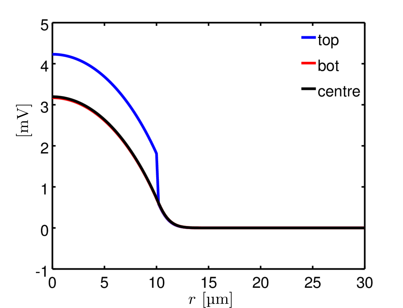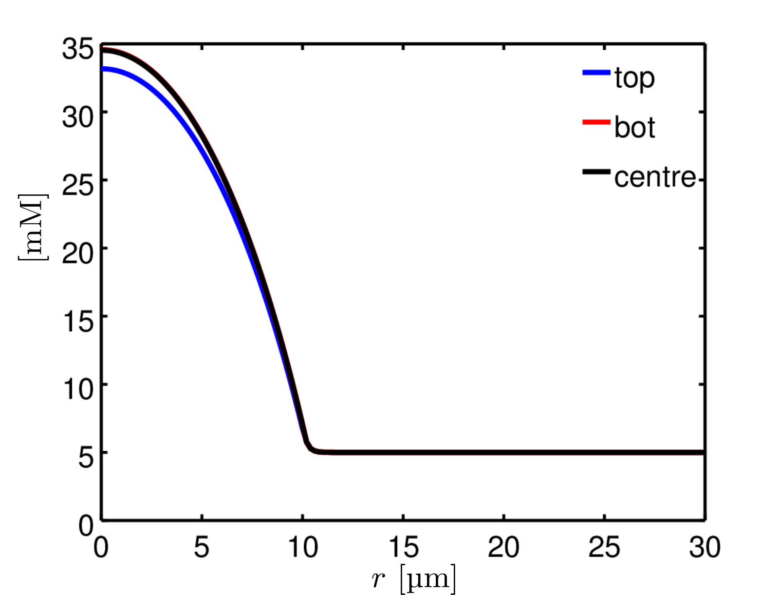3.1, based on the simulations of the previous sections and on asymptotic analysis (see [32]), we set $H\simeq 2\lambda_{Debye}\simeq$ $1.6\text{\,}\mathrm{nm}$ .

Simulation results obtained with the reduced model are shown in Fig. 26, where we immediately notice that the capacitive couplings obtained with 3D simulations of Sect. 5.2 are well reproduced. As observed in Sect. 3.1 and in the spatial distributions of Sect. 5.3, the quantities of interest in $\Omega_{r}^{ef}$ are not expected to sensibly vary along $z$ . This solution behavior is confirmed by the radial distributions of Fig. 26: potential $\overline{\varphi}$ and concentrations $\overline{c}_{i}$ are perfectly superimposed on the distributions of the top and bottom quantities in the free part. We observe a very fast decay in $\Omega_{r}^{ef}$ , as expected and as the one obtained in the simulation results shown in Fig. 12.

Having computed the averaged and the top and bottom values of the dependent variables, we can also reconstruct their $z$ -dependence, at a fixed point $\bar{r}$ , using the following post-processing formulas:


(17a)			$\displaystyle\varphi(\bar{r},z)=\overline{\varphi}(z,\bar{r})+\left.\left(\dfrac{\varphi_{top}(\bar{r},z)-\overline{\varphi}(\bar{r},z)}{H}\right)\right\|_{z\in\Omega_{1}}+\left.\left(\dfrac{\overline{\varphi}(\bar{r},z)-\varphi_{bot}(\bar{r},z)}{H}\right)\right\|_{z\in\Omega_{3}}$
(17b)			$\displaystyle c_{i}(\bar{r},z)=\overline{c}_{i}\exp\left(-z_{i}\dfrac{\varphi(\bar{r},z)-\overline{\varphi}(\bar{r},z)}{V_{th}}\right),$

where $\Omega_{1}$ and $\Omega_{3}$ are the boundary layer subdomains (see Fig. 7). The reconstruction of $\varphi(r=0,z)$ and of $c_{K}(r=0,z)$ is illustrated in Fig. 27 and we see that the major term in the electrolyte system behavior is the capacitive coupling with the cell membrane.

The above obtained results allow us to conclude that the reduced mathematical model of Sect. 3.1 is valid, because its predictions favorably agree with those of the 3D model, but with a much smaller amount of degrees of freedom.

5.6.2. Validation of the 2.5D model against exact solutions

In this section we analyze a biophysical setting similar to that presented in [36], where the authors derive the exact profiles of potential and ion concentrations in radial coordinates under the assumption of axial symmetry. Their model refers to the middle plane of a cleft between a cell and a substrate as in the general setup described in Sect. 3, but under the following simplifications:

•

ions are assumed to flow only in the radial direction, so that $j_{i,\phi}=j_{i,z}=0$ , and no spatial dependence on $\phi$ and $z$ is assumed. The radial coordinate $r$ is taken in the interval $[0,R]$ ( $R$ being the cell radius);
•

the influx of $\text{K}^{+}$ ion charge per volume and per time is given by $\lambda_{K}=j_{K}^{tm}/\delta_{j}$ , where $\delta_{j}$ is the cleft width and $j_{K}^{tm}$ is the potassium current density through the membrane, here assumed to be constant. Therefore in Eq. (6a) we only have $f^{top}_{K}=\lambda_{K}$ ;
•

there is no influence on the flux of ions inside the cleft from the two interfaces (the cell-cleft and the chip-cleft interfaces), neglecting the capacitive couplings described in Sect. 2.3. This gives $g^{top}=g^{bot}=0$ in Eq. (6c);
•

only the stationary case is considered, meaning that all quantities are independent of time.

(a) Potential

(b) Concentrations

Figure 28. On the left: radial profile of the potential

\varphi\left(r\right)

. On the right: radial profile of the changes of ion concentrations with respect to their bath values

c_{i}\left(r\right)-c_{i}^{bath}

. Results obtained with a source term

\lambda_{K}=

11\text{\,}\mathrm{pA}\text{\,}{\mathrm{\SIUnitSymbolMicro m}}^{-2}

and a cell radius

R=

15\text{\,}\mathrm{\SIUnitSymbolMicro m}

as in [36].

Fig. 28 shows the computed distributions of potential and ion concentrations under the cell. By inspection on the analytical solutions reported in [36] it can be seen that our results are in excellent agreement with the latter solutions. Convergence of the finite element solution as a function of the radial mesh size $h$ is reported in Fig. 29 where a quadratic rate can be observed before the occurrence of error saturation due to the nonlinear solver tolerance. This result, obtained in the solution of a nonlinear problem, confirms the convergence analysis of Sect. 5.1, carried out on a linear model problem.

Figure 29. Log-log plot of the maximum norm of the discretization error

\varphi-\varphi_{h}

Under the hypotheses illustrated above, the potential variation at $r=0$ is quite small (less than $1\text{\,}\mathrm{m}\mathrm{V}$ ) and the absolute changes of ion concentrations for $\text{Cl}^{-}$ and $\text{Na}^{+}$ are quite small too, except for $\text{K}^{+}$ ion concentration, from 5 mM to 8 mM.

(a) Potential

\varphi(t,r=0)

(b) Concentrations

c_{i}(t,r=0)-c_{i}^{bath}

Figure 30. Time variation of the potential and of the concentrations with respect to their bath values, at the center of the junction.

We also conduct a time dependent simulation of this experimental setup, redefining the transmembrane current as $\lambda_{K}\left(t\right)=\lambda_{K}H\left(t\right)$ , where $\lambda_{K}$ is the constant current used in the static simulation and $H\left(t\right)$ is the Heaviside function. With this mathematical definition of potassium injection, we consider an instantaneous opening of the $\text{K}^{+}$ channels at $t=0$ , which leads to a time variation of the quantities $\varphi$ and $c_{i}$ (see Fig. 30, where we show the variation of these functions evaluated at $r=0$ ). Transients are exhausted in about $150\text{\,}\mathrm{m}\mathrm{s}$ , in agreement with the results of [45], while the steady-state values of $\varphi$ and $c_{i}$ agree well with those computed in the static case shown in Fig. 28.

5.6.3. Validation of the Area-Contact model

In this concluding section we compare the results obtained with the Area-Contact (A-C) model proposed in Sect. 3.2 with the results of [8], which we refer to for all physical data and details of the electrical equivalent circuits used to determine the time evolution of ion concentrations in the cleft. To this purpose, we conduct a first simulation considering given concentrations $c_{i}$ constant in time and only solving Eq. (13) (2D electrical model). Then, we conduct a second simulation accounting for ion dynamics, by adding an ODE system for the ionic concentrations (2D electrodiffusion model). In both cases the integral mean $V_{J}$ is computed as in (13c). The considered electrophysiological experiment is a voltage clamp stimulation with the depolarizing pulse shown by Fig. 31(a) and the values of model parameters are the same as in [8].

As demonstrated by Fig. 31(b), the 2D electrical model accounts only for the fast response of the system, with a dynamics determined by the electrical time constant $\tau=\left(C_{M}+C_{S}\right)/\sigma\simeq$ $1.0944\text{\,}\mathrm{\SIUnitSymbolMicro S}$ ( $\sigma=q\sum_{i=1}^{M}|z_{i}|\mu_{i}c_{i}^{bath}\delta_{J}$ being the global cleft conductance): when the cell is depolarized, almost instantaneously the potential goes to a value around $2\text{\,}\mathrm{m}\mathrm{V}$ . The 2D electrodiffusion model, instead, describing the time variation of $c_{i}$ , accounts also for the slow component, as shown by Figs. 31(c) and 31(d): both potential and concentrations have transients with a time constant in the order of milliseconds, as expected (we have expressed the changes of extracellular ion concentrations in the junction as Nernst potentials between junction and bath). The integral mean of the electrical potential $\varphi$ increases fast to a value around $2.5\text{\,}\mathrm{m}\mathrm{V}$ and subsequently decays to a stationary level around $1.5\text{\,}\mathrm{mV}$ and the potassium concentration increases from $5$ mM to $17$ mM, giving a Nernst potential $V_{J}^{K}\simeq$ $-27\text{\,}\mathrm{m}\mathrm{V}$ in the junction. Notably, all results are in excellent agreement with those reported by Brittinger and Fromherz in [8]. Finally, the spatial distributions of the potential $\varphi$ computed by the 2D electrical and electrodiffusion models, and used to determine $V_{J}$ in (13c), are reported in Fig. 32. The resulting parabolic shape is in very good agreement with the behavior shown by the 3D results of Sect. 3.2.

6. Conclusions and Future Perspectives

In this article we have addressed the mathematical modeling and numerical simulation of ion electrodiffusion in bio-hybrid devices. This subject is of paramount importance in the wider scientific context of neuroelectronics, where the main aim is to actually realize devices consisting of the integration of biological tissues with solid-state integrated electronic circuits.

In this treatise we have illustrated a suitable mathematical characterization of bio-electronic interfaces, investigating different possible modeling hypotheses on the coupling between the two different environments (cell and electronic device) and on the derivation of model dimensional reductions, performed to decrease the computational simulation effort. A hierarchy of multiscale models has been therefore presented and extensively validated with a broad range of numerical computations, obtaining sensible results and comparing them with literature and experiments.

This mathematical description has also been applied to complex configurations and has proved to be able to simulate the interactions between multiple cells and multiple devices. Even if the present work is not a faithful copy of a real-world biophysical setting, it can be considered a first step for the construction of mathematical models to be used in the design of actual devices.

Clearly, future research is needed to provide a better description of the complex multiscale/multiphysics problem object of our investigation. Among possible developments, we mention:

•

a more accurate modeling of the electronic substrate, which can be useful in studying different types of stimulation, for example a different polarization of the chip influencing the cell;
•

a model for the chemical binding mechanism of the ions to the electronic substrate is also required, in order to fully describe the EOSFET device;
•

a coupling between electro-chemical and fluid-mechanical systems, in order to account for the forces due to pressure differences and flow in the aqueous medium;
•

a more realistic description of the problem geometry, with full three-dimensional computations including the intracellular fluid can be useful to faithfully reproduce the entire phenomena;
•

an application of the computational model to the simulation of electrophysiological experiments in current-clamp conditions.

The above mentioned improvements, particularly, the study of the current-clamp protocol, should give the realistic chance to go further in the study of the interactions between multiple cells, maybe introducing a neural network and simulating a whole brain slice, as in the experimental results of [26, 47].

Acknowledgments

Matteo Porro and Riccardo Sacco were supported by Gruppo Nazionale per il Calcolo Scientifico of Istituto Nazionale di Alta Matematica “F. Severi”. Thierry Nieus was partially supported by the SI-CODE project of the Future and Emerging Technologies (FET) programme within the Seventh Framework Programme for Research of The European Commission, under FET-Open grant number: FP7-284553.

References

[1] E. Abbate. Hierarchical multiscale modeling and simulation of bio-electronic interfaces. Master’s thesis, Politecnico di Milano, 2014.
[2] R.E. Bank, W.M. Coughran Jr, and L.C. Cowsar. The finite volume Scharfetter-Gummel method for steady convection diffusion equations. Computing and Visualization in Science, 1(3):123–136, 1998.
[3] F. Bosisio, S. Micheletti, and R. Sacco. A discretization scheme for an extended drift-diffusion model including trap-assisted phenomena. Journal of Computational Physics, 159(2):197–212, 2000.
[4] M. Brera. Multiphysics/multiscale computational modeling in neuroelectronics. Master’s thesis, Politecnico di Milano, 2009.
[5] M. Brera, J.W. Jerome, Y. Mori, and R. Sacco. A conservative and monotone mixed-hybridized finite element approximation of transport problems in heterogeneous domains. Computer Methods in Applied Mechanics and Engineering, 199(41):2709–2720, 2010.
[6] F. Brezzi, L. D. Marini, and P. Pietra. Numerical simulation of semiconductor devices. Computer Methods in Applied Mechanics and Engineering, 75(1–3):493 – 514, 1989.
[7] F. Brezzi, L.D. Marini, and P. Pietra. Two-dimensional exponential fitting and applications to drift-diffusion models. SIAM Journal on Numerical Analysis, 26(6):1342–1355, 1989.
[8] M. Brittinger and P. Fromherz. Field-effect transistor with recombinant potassium channels: fast and slow response by electrical and chemical interactions. Applied Physics A, 81(3):439–447, 2005.
[9] M. Cogliati and M. Porro. Third generation solar cells: modeling and simulations. Master’s thesis, Politecnico di Milano, 2009.
[10] C. de Falco. Quantum–corrected drift–diffusion models and numerical simulation of nanoscale semiconductor devices. PhD thesis, Università degli Studi di Milano, 2006.
[11] C. de Falco, M. Porro, R. Sacco, and M. Verri. Multiscale modeling and simulation of organic solar cells. Computer Methods in Applied Mechanics and Engineering, 245 - 246(0):102 – 116, 2012.
[12] R.S. Eisenberg. Ionic channels in biological membranes: Natural nanotubes. Accounts of Chemical Research, 31(3):117–123, 1998.
[13] R.S. Eisenberg. From structure to function in open ionic channels. Journal of Membrane Biology, 171:1–24, 1999.
[14] R.S. Eisenberg. Ions in fluctuating channels: transistors alive. Fluct. Noise Lett., 11, 2012.
[15] G. Ermentrout and D. Terman. Mathematical Foundations of Neuroscience. Springers, 2010.
[16] E. Ferrea, A. Maccione, L. Medrihan, T. Nieus, D. Ghezzi, P. Baldelli, F. Benfenati, and L. Berdondini. Large-scale, high-resolution electrophysiological imaging of field potentials in brain slices with microelectronic multielectrode arrays. Front Neural Circuits, 6(80):1–8, 2012.
[17] P. Fromherz, S. Eick, and B. Hofmann. Neuroelectronic Interfacing with Semiconductor Chips. In R. Waser, editor, Nanoelectronics and Information Technology 3rd, pages 847–868. Weinheim, Berlin, 2012.
[18] C.L. Gardner, J.R. Jones, S.M. Baer, and S. Chang. Simulation of the ephaptic effect in the cone–horizontal cell synapse of the retina. SIAM Journal on Applied Mathematics, 73(2):636–648, 2013.
[19] E. Gatti, S. Micheletti, and R. Sacco. A new Galerkin framework for the drift-diffusion equation in semiconductors. East West Journal of Numerical Mathematics, 6:101–136, 1998.
[20] D. Ghezzi, M. R. Antognazza, M. Dal Maschio, E. Lanzarini, F. Benfenati, and G. Lanzani. A hybrid bioorganic interface for neuronal photoactivation. Nature Communications, 2:166, 2011.
[21] D.C. Grahame. The electrical double layer and the theory of electrocapillarity. Chemical Reviews, 41(3):441–501, 1947.
[22] H.K. Gummel. A self-consistent iterative scheme for one-dimensional steady state transistor calculations. IEEE Transactions on Electron Devices, 11(10):455–465, 1964.
[23] B. Hille. Ion channels of excitable membranes, volume 507. Sinauer Sunderland, MA, 2001.
[24] A.L. Hodgkin and A.F. Huxley. Currents carried by sodium and potassium ions through the membrane of the giant axon of loligo. The Journal of physiology, 116(4):449, 1952.
[25] A.L. Hodgkin and A.F. Huxley. A quantitative description of membrane current and its application to conduction and excitation in nerve. The Journal of physiology, 117(4):500, 1952.
[26] M. Hutzler, A. Lambacher, B. Eversmann, M. Jenkner, R. Thewes, and P. Fromherz. High-resolution multitransistor array recording of electrical field potentials in cultured brain slices. Journal of neurophysiology, 96(3):1638–1645, 2006.
[27] J.W. Jerome. Analysis of charge transport. Springer Berlin, 1996.
[28] N. Joye, A. Schmid, and Y. Leblebici. An electrical model of the cell-electrode interface for high-density microelectrode arrays. In Engineering in Medicine and Biology Society, 2008. EMBS 2008. 30th Annual International Conference of the IEEE, pages 559–562. IEEE, 2008.
[29] J. Keener and J. Sneyd. Mathematical Physiology. Springer-Verlag, 2009.
[30] T. Kerkhoven. A spectral analysis of the decoupling algorithm for semiconductor simulation. SIAM Journal on Numerical Analysis, 25(6):1299–1312, 1988.
[31] R.D. Lazarov and L.T. Zikatanov. An exponential fitting scheme for general convection-diffusion equations on tetrahedral meshes. arXiv preprint arXiv:1211.0869, 2012.
[32] Y. Mori. A three-dimensional model of cellular electrical activity. PhD thesis, New York University, 2006.
[33] Y. Mori and C.S. Peskin. A numerical method for cellular electrophysiology based on the electrodiffusion equations with internal boundary conditions at the membrane. Communications in Applied Mathematics and Computational Sciences, 4:85–134, 2009.
[34] C. Moulin, A. Glière, D. Barbier, S. Joucla, B. Yvert, P. Mailley, and R. Guillemaud. A new 3-d finite-element model based on thin-film approximation for microelectrode array recording of extracellular action potential. IEEE Transactions on Biomedical Engineering, 55(2):683–692, 2008.
[35] E. Neher. Molecular biology meets microelectronics. Nature Biotechnology, 19(2):114–114, 2001.
[36] M. Pabst, G. Wrobel, S. Ingebrandt, F. Sommerhage, and A. Offenhäusser. Solution of the Poisson-Nernst-Planck equations in the cell-substrate interface. The European Physical Journal E, 24(1):1–8, 2007.
[37] A. Quarteroni and A. Valli. Domain decomposition methods for partial differential equations. Numerical Mathematics Scientific Computation, Clarendon Press, 1999.
[38] A. Quarteroni and A. Valli. Numerical approximation of partial differential equations, volume 23. Springer, 2008.
[39] I. Rubinstein. Electro-diffusion of ions, volume 11. SIAM, 1990.
[40] D.L. Scharfetter and H.K. Gummel. Large-signal analysis of a silicon Read diode oscillator. IEEE Transactions on Electron Devices, 16(1):64–77, 1969.
[41] J.W. Slotboom. Computer-aided two-dimensional analysis of bipolar transistors. IEEE Transactions on Electron Devices, 20(8):669–679, Aug 1973.
[42] M. Voelker and P. Fromherz. Signal transmission from individual mammalian nerve cell to field-effect transistor. Small, 1:206–210, 2005.
[43] R. Waser. Nanoelectronics and information technology. John Wiley & Sons, 2012.
[44] I. Willner and E. Katz. Bioelectronics: from theory to applications. John Wiley & Sons, 2006.
[45] G. Wrobel, R. Seifert, S. Ingebrandt, H. Enderlein, J.and Ecken, A. Baumann, U.B. Kaupp, and A. Offenhäusser. Cell-transistor coupling: investigation of potassium currents recorded with p-and n-channel fets. Biophysical journal, 89(5):3628–3638, 2005.
[46] J. Xu and L. Zikatanov. A monotone finite element scheme for convection-diffusion equations. Mathematics of Computation of the American Mathematical Society, 68(228):1429–1446, 1999.
[47] G. Zeck and P. Fromherz. Noninvasive neuroelectronic interfacing with synaptically connected snail neurons immobilized on a semiconductor chip. Proceedings of the National Academy of Sciences, 98(18):10457–10462, 2001.

(5g)		$\displaystyle c_{i}^{top}:=\left.c_{i}\right\|_{\Sigma_{top}}$		$\displaystyle c_{i}^{bot}:=\left.c_{i}\right\|_{\Sigma_{bot}}$
(5h)		$\displaystyle\varphi_{top}:=\left.\varphi\right\|_{\Sigma_{top}}$		$\displaystyle\varphi_{bot}:=\left.\varphi\right\|_{\Sigma_{bot}}.$