跳到论文正文
W Papers独立论文阅读器 arXiv:1501.04326 论文正文 计算阅读时间 · 0%
引用这篇论文根据当前论文元数据生成,正式投稿前建议核对。


License: arXiv.org perpetual non-exclusive license
arXiv:1501.04326v2 [math.NA] 17 Jul 2016

The spherical Radon transform with centers on cylindrical surfaces

Markus Haltmeier Email: markus.haltmeier@uibk.ac.at Address: Department of Mathematics, University of Innsbruck, Technikestraße 13, A-6020 Innsbruck, Austria    Sunghwan Moon Email: shmoon@unist.ac.kr Address: Department of Mathematical Sciences, Ulsan National Institute of Science and Technology, Ulsan 44919, Republic of Korea Corresponding author: Corresponding author
Abstract

Recovering a function from its spherical Radon transform with centers of spheres of integration restricted to a hypersurface is at the heart of several modern imaging technologies, including SAR, ultrasound imaging, and photo- and thermoacoustic tomography. In this paper we study an inversion of the spherical Radon transform with centers of integration restricted to cylindrical surfaces of the form Γ×ℝm\Gamma\times\mathbb{R}^{m}, where Γ\Gamma is a hypersurface in ℝn\mathbb{R}^{n}. We show that this transform can be decomposed into two lower dimensional spherical Radon transforms, one with centers on Γ\Gamma and one with a planar center-set in ℝm+1\mathbb{R}^{m+1}. Together with explicit inversion formulas for the spherical Radon transform with a planar center-set and existing algorithms for inverting the spherical Radon transform with a center-set Γ\Gamma, this yields reconstruction procedures for general cylindrical domains. In the special case of spherical or elliptical cylinders we obtain novel explicit inversion formulas. For three spatial dimensions, these inversion formulas can be implemented efficiently by backprojection type algorithms only requiring 𝒪⁡(𝙽4/3)\mathcal{O}({\tt N}^{4/3}) floating point operations, where 𝙽{\tt N} is the total number of unknowns to be recovered. We present numerical results demonstrating the efficiency of the derived algorithms.

Keywords: 
Spherical means, Radon transform, inversion, reconstruction formula
MSC
44A12 , 45Q05, 35L05, 92C55

1 Introduction

Let Γ\Gamma be a hypersurface in ℝn\mathbb{R}^{n}. In this paper we study the spherical Radon transform with a center-set Γ×ℝm\Gamma\times\mathbb{R}^{m} that maps a function f:ℝn+m→ℝf\colon\mathbb{R}^{n+m}\to\mathbb{R} to the spherical integrals

(𝐌x,y​f)​(x,y,r)≔1|𝕊n+m−1|​∫𝕊n+m−1f⁡((x,y)+r​ω)​dS⁡(ω) for ​(x,y,r)∈Γ×ℝm+1.(\mathbf{M}_{x,y}f)(x,y,r)\coloneqq\frac{1}{\lvert\mathbb{S}^{{n+m}-1}\rvert}\int_{\mathbb{S}^{{n+m}-1}}f((x,y)+r\omega)\dS(\omega)\quad\text{ for }(x,y,r)\in\Gamma\times\mathbb{R}^{m+1}\,.

Here |r|\lvert r\rvert and (x,y)∈Γ×ℝm(x,y)\in\Gamma\times\mathbb{R}^{m} are the radius and the center of the sphere of integration, respectively, 𝕊n+m−1\mathbb{S}^{{n+m}-1} is the unit sphere in ℝn+m\mathbb{R}^{n+m}, and |𝕊n+m−1|\lvert\mathbb{S}^{{n+m}-1}\rvert is the total surface area of 𝕊n+m−1\mathbb{S}^{{n+m}-1}. Note that x,yx,y as subscripts of (𝐌x,y​f)​(x,y,r)(\mathbf{M}_{x,y}f)(x,y,r) indicate the variables in which the spherical Radon transform is applied, while in the argument they are placeholders for the actual data points. For example, evaluating the spherical Radon transform at (x,y,r)=(0,0,0)(x,y,r)=(0,0,0) gives (𝐌x,y​f)​(0,0,0)(\mathbf{M}_{x,y}f)(0,0,0). Similar notions will be used for auxiliary transforms introduced below; these suggestive notations are used to facilitate the readability of the manuscript.

Recovering a function from its spherical Radon transform with centers restricted to a hypersurface is crucial for the recently developed thermoacoustic and photoacoustic tomography [1, 2]. It is also relevant for other imaging technologies such SAR imaging [3, 4] or ultrasound tomography [5].

Explicit inversion formulas for reconstructing ff from its spherical Radon transform are of theoretical as well of practical importance. For example, they serve as theoretical basis of backprojection-type reconstruction algorithms frequently used in practice. However, explicit inversion formulas are only known for some special center-sets. Such formulas exist for the case where the center-set is a hyperplane [6, 7, 8, 9, 10, 11] or a sphere [12, 13, 14, 15, 16]. More recently, closed-form inversions have also been derived for the cases of elliptically shaped center-sets (see [17, 18, 19, 20, 21, 22]), certain quadrics [23, 24], oscillatory algebraic sets [25], and corner-like domains [26].

Refer to caption
Refer to caption
Figure 1.1: Left: A phantom consisting of a superposition of three balls. Right: 3D reconstruction from its spherical Radon transform on a cylinder in ℝ3\mathbb{R}^{3} using the inversion formula (2) derived in Section 3.

1.1 Main contribution

In this paper we present a general approach for deriving reconstruction algorithms and inversion formulas for the spherical Radon transform on cylindrical surfaces yielding inversion formulas for the center-set Γ×ℝm\Gamma\times\mathbb{R}^{m}, provided that an inversion formula is known for the center-set Γ\Gamma. Our approach is based on the observation that the spherical Radon transform with a center-set Γ×ℝm\Gamma\times\mathbb{R}^{m} can be written as the composition of a spherical Radon transform with a center-set Γ⊆ℝn\Gamma\subseteq\mathbb{R}^{n} and another spherical Radon transform with a planar center-set in ℝm+1\mathbb{R}^{m+1} (see Theorem 2.3). Recall that inversion formulas for the spherical Radon transform with a planar center-set are well known. Consequently, if an inversion formula is available for the center-set Γ⊆ℝn\Gamma\subseteq\mathbb{R}^{n}, then this factorization yields an inversion formula for 𝐌x,y\mathbf{M}_{x,y}. As explicit inversion formulas are in particular known for spherical and elliptical center-sets, we obtain new analytic inversion formulas for spherical or elliptical cylinders (Theorems 3.1 and 3.2). A reconstruction result with one of our inversion formulas for an elliptical cylinder is shown in Figure 1.1.

We emphasize, that our factorization approach can also be combined with any other reconstruction algorithm for the spherical means, such as time reversal [27, 28, 29] or series expansion methods [30, 31], that can be used for the case where Γ\Gamma is the boundary of a general bounded domain.

1.2 Outline

The rest of this paper is organized as follows. In Section 2 we show that the spherical Radon transform with centers on Γ×ℝm\Gamma\times\mathbb{R}^{m} can be decomposed in two partial spherical Radon transforms, one with a center-set Γ\Gamma and one with a planar center-set in ℝm+1\mathbb{R}^{m+1}; see Theorem 2.3. In Section 3 we apply the factorization approach to derive novel explicit inversion formulas for the case where Γ×ℝm\Gamma\times\mathbb{R}^{m} is an elliptical or circular cylinder; see Theorems 3.1 and 3.2. In Section 4 we derive filtered backprojection algorithms based on the inversion formulas for elliptical cylinders in ℝ3\mathbb{R}^{3} and present numerical results. The paper concludes with a short discussion in Section 5.

2 Decomposition of the spherical Radon transform

We study the spherical Radon transform with centers on a cylinder Γ×ℝm\Gamma\times\mathbb{R}^{m}, where Γ⊆ℝn\Gamma\subseteq\mathbb{R}^{n} is any smooth hypersurface with n,m∈ℕn,m\in\mathbb{N} and n≥2n\geq 2. It will be convenient to identify ℝn+m≃ℝn×ℝm\mathbb{R}^{{n+m}}\simeq\mathbb{R}^{n}\times\mathbb{R}^{m} and to write any point in ℝn+m\mathbb{R}^{{n+m}} in the form (x,y)∈ℝn×ℝm(x,y)\in\mathbb{R}^{n}\times\mathbb{R}^{m}.

Definition 2.1 (Spherical Radon transform with a cylindrical center-set).

Let f∈Lloc1​(ℝn+m)f\in L^{1}_{\rm loc}(\mathbb{R}^{n+m}). The spherical Radon transform of ff with a cylindrical center-set Γ×ℝm\Gamma\times\mathbb{R}^{m} is defined by

𝐌x,y​f:Γ×ℝm+1\displaystyle\mathbf{M}_{x,y}f\colon\Gamma\times\mathbb{R}^{m+1} →ℝ\displaystyle\to\mathbb{R}
(x,y,r)\displaystyle(x,y,r) ↦1|𝕊n+m−1|​∫𝕊n+m−1f⁡((x,y)+r​ω)​dS⁡(ω).\displaystyle\mapsto\frac{1}{\lvert\mathbb{S}^{{n+m}-1}\rvert}\int_{\mathbb{S}^{{n+m}-1}}f\left((x,y)+r\omega\right)\dS(\omega)\,.

In the following we show that 𝐌x,y\mathbf{M}_{x,y} can be written as the product of two lower dimensional spherical Radon transforms, one with a center-set Γ\Gamma in ℝn\mathbb{R}^{n} and one with a planar center-set in ℝm+1\mathbb{R}^{m+1}. These partial spherical Radon transforms are defined as follows.

Definition 2.2 (Partial spherical Radon transforms).

  1. (a)

    For f∈Lloc1​(ℝn+m)f\in L^{1}_{\rm loc}(\mathbb{R}^{n+m}) we define

    𝐌x​f:Γ×ℝm+1→ℝ:(x,y,s)↦1|𝕊n−1|​∫𝕊n−1f⁡(x+s​ω1,y)​dS⁡(ω1).\mathbf{M}_{x}f\colon\Gamma\times\mathbb{R}^{m+1}\to\mathbb{R}\colon(x,y,s)\mapsto\frac{1}{\lvert\mathbb{S}^{n-1}\rvert}\int_{\mathbb{S}^{n-1}}f(x+s\omega_{1},y)\dS(\omega_{1})\,.
  2. (b)

    For h∈Lloc1​(Γ×ℝm+1)h\in L^{1}_{\rm loc}(\Gamma\times\mathbb{R}^{m+1}) we define

    𝐌y,s​h:Γ×ℝm+1→ℝ:(x,y,r)↦1|𝕊m|​∫𝕊mh⁡(x,(y,0)+r​σ)​dS⁡(σ).\mathbf{M}_{y,s}h\colon\Gamma\times\mathbb{R}^{m+1}\to\mathbb{R}\colon(x,y,r)\mapsto\frac{1}{\lvert\mathbb{S}^{m}\rvert}\int_{\mathbb{S}^{m}}h(x,(y,0)+r\sigma)\dS(\sigma)\,.

The operators 𝐌x\mathbf{M}_{x} and 𝐌y,s\mathbf{M}_{y,s} are partial spherical Radon transforms, where the subscripts indicate the variables in which the integration is applied. By definition, 𝐌x,y​f\mathbf{M}_{x,y}f, 𝐌x​f\mathbf{M}_{x}f, and 𝐌y,s​h\mathbf{M}_{y,s}h are even in the last variable.

Theorem 2.3 (Decomposition).

For every f∈Lloc1​(ℝn+m)f\in L^{1}_{\rm loc}(\mathbb{R}^{n+m}) we have

𝐌x,y​f=Cn,m​|r|1−n​𝐌y,s​(|s|n−1​𝐌x​f)w​i​t​hCn,m≔12​|𝕊m|​|𝕊n−1||𝕊n+m−1|.\mathbf{M}_{x,y}f=C_{n,m}\,\lvert r\rvert^{1-n}\mathbf{M}_{y,s}\left(\lvert s\rvert^{n-1}\mathbf{M}_{x}f\right)\quad{with}\quad C_{n,m}\coloneqq\frac{1}{2}\,\frac{\lvert\mathbb{S}^{m}\rvert\,\lvert\mathbb{S}^{n-1}\rvert}{\lvert\mathbb{S}^{{n+m}-1}\rvert}\,. (1)
Proof.

We use standard spherical coordinates Φ:(0,2​π)×(0,π)n−2×(0,π)m→𝕊n+m−1\Phi\colon(0,2\pi)\times(0,\pi)^{n-2}\times(0,\pi)^{m}\to\mathbb{S}^{{n+m}-1} written in the form Φ⁡(α,β)=(Φ1​(α)​sin⁡(β1)​…​sin⁡(βm),Φ2​(β))\Phi(\alpha,\beta)=(\Phi_{1}(\alpha)\sin(\beta_{1})\dots\sin(\beta_{m}),\Phi_{2}(\beta)) for α∈(0,2​π)×(0,π)n−2\alpha\in(0,2\pi)\times(0,\pi)^{n-2} and β∈(0,π)m\beta\in(0,\pi)^{m}, where

Φ1​(α)≔[sin(α1)sin(α2)⋯sin(αn−1)cos(α1)sin(α2)⋯sin(αn−1)⋮cos⁡(αn−2)​sin⁡(αn−1)cos⁡(αn−1)]andΦ2​(β)≔[cos(β1)sin(β2)sin(β3)⋯sin(βm)cos(β2)sin(β3)⋯sin(βm)⋮cos⁡(βm−1)​sin⁡(βm)cos⁡(βm)].\Phi_{1}(\alpha)\coloneqq\left[\begin{array}[]{r}\sin(\alpha_{1})\sin(\alpha_{2})\cdots\sin(\alpha_{n-1})\\ \cos(\alpha_{1})\sin(\alpha_{2})\cdots\sin(\alpha_{n-1})\\ \vdots\\ \cos(\alpha_{n-2})\sin(\alpha_{n-1})\\ \cos(\alpha_{n-1})\end{array}\right]\quad\text{and}\quad\Phi_{2}(\beta)\coloneqq\left[\begin{array}[]{r}\cos(\beta_{1})\sin(\beta_{2})\sin(\beta_{3})\cdots\sin(\beta_{m})\\ \cos(\beta_{2})\sin(\beta_{3})\cdots\sin(\beta_{m})\\ \vdots\\ \cos(\beta_{m-1})\sin(\beta_{m})\\ \cos(\beta_{m})\end{array}\right]\,.

Notice that Φ1:(0,2​π)×(0,π)n−2→𝕊n−1\Phi_{1}\colon(0,2\pi)\times(0,\pi)^{n-2}\to\mathbb{S}^{n-1} is the standard parameterization of 𝕊n−1\mathbb{S}^{n-1} using spherical coordinates. Further, not that dSn−1(α)=sin(α2)…sin(αn−1)n−2d​α\dS_{n-1}(\alpha)=\sin(\alpha_{2})\dots\sin(\alpha_{n-1})^{n-2}\dalpha is the surface element on 𝕊n−1\mathbb{S}^{n-1} and sin(β1)n−1…sin(βm)n+m−2dSn−1(α)d​β\sin(\beta_{1})^{n-1}\dots\sin(\beta_{m})^{{n+m}-2}\dS_{n-1}(\alpha)\dbeta the surface element on 𝕊n+m−1\mathbb{S}^{{n+m}-1}. Expressing the spherical Radon transform 𝐌y,s\mathbf{M}_{y,s} in terms of integrals over the parameter set (0,2​π)×(0,π)n−2×(0,π)m(0,2\pi)\times(0,\pi)^{n-2}\times(0,\pi)^{m} therefore yields

(𝐌x,y​f)​(x,y,r)\displaystyle(\mathbf{M}_{x,y}f)(x,y,r)
=1|𝕊n+m−1|​∫(0,π)m∫(0,2​π)×(0,π)n−2f⁡(x+r​sin⁡(β1)​…​sin⁡(βm)​Φ1​(α),y+r​Φ2​(β))\displaystyle=\frac{1}{\lvert\mathbb{S}^{{n+m}-1}\rvert}\int_{(0,\pi)^{m}}\int_{(0,2\pi)\times(0,\pi)^{n-2}}f\left(x+r\sin(\beta_{1})\dots\sin(\beta_{m})\Phi_{1}(\alpha),y+r\Phi_{2}(\beta)\right)
×sin(β1)n−1…sin(βm)n+m−2dSn−1(α)d​β\displaystyle\hskip 137.9979pt\times\sin(\beta_{1})^{n-1}\dots\sin(\beta_{m})^{{n+m}-2}\dS_{n-1}(\alpha)\dbeta
=|𝕊n−1||𝕊n+m−1|∫(0,π)m(𝐌xf)(x,y+rΦ2(β),rsin(β1)⋯sin(βm))sin(β1)n−1…sin(βm)n+m−2d​β\displaystyle=\frac{\lvert\mathbb{S}^{n-1}\rvert}{\lvert\mathbb{S}^{{n+m}-1}\rvert}\int_{(0,\pi)^{m}}(\mathbf{M}_{x}f)\left(x,y+r\Phi_{2}(\beta),r\sin(\beta_{1})\cdots\sin(\beta_{m})\right)\sin(\beta_{1})^{n-1}\dots\sin(\beta_{m})^{{n+m}-2}\dbeta
=|𝕊n−1|​|r|1−n|𝕊n+m−1|∫(0,π)m(𝐌xf)(x,y+rΦ2(β),rsin(β1)…sin(βm))|r|n−1sin(β1)n−1⋯sin(βm)n+m−2d​β\displaystyle=\frac{\lvert\mathbb{S}^{n-1}\rvert\,\lvert r\rvert^{1-n}}{\lvert\mathbb{S}^{{n+m}-1}\rvert}\int_{(0,\pi)^{m}}(\mathbf{M}_{x}f)\left(x,y+r\Phi_{2}(\beta),r\sin(\beta_{1})\dots\sin(\beta_{m})\right)\lvert r\rvert^{n-1}\sin(\beta_{1})^{n-1}\cdots\sin(\beta_{m})^{{n+m}-2}\dbeta
=|𝕊n−1|​|r|1−n|𝕊n+m−1|∫(0,π)m(|s|n−1𝐌xf)(x,y+rΦ2(β),rsin(β1)…sin(βm))sin(β2)…sin(βm)m−1d​β.\displaystyle=\frac{\lvert\mathbb{S}^{n-1}\rvert\,\lvert r\rvert^{1-n}}{\lvert\mathbb{S}^{{n+m}-1}\rvert}\int_{(0,\pi)^{m}}\left(\lvert s\rvert^{n-1}\mathbf{M}_{x}f\right)\left(x,y+r\Phi_{2}(\beta),r\sin(\beta_{1})\dots\sin(\beta_{m})\right)\sin(\beta_{2})\dots\sin(\beta_{m})^{m-1}\dbeta\,.

Next notice that β↦(Φ2​(β),sin⁡(β1)​…​sin⁡(βm))\beta\mapsto\left(\Phi_{2}(\beta),\sin(\beta_{1})\dots\sin(\beta_{m})\right) is a parameterization of 𝕊+m≔𝕊m∩{(y,s)∈ℝm+1:s≥0}\mathbb{S}^{m}_{+}\coloneqq\mathbb{S}^{m}\cap\{(y,s)\in\mathbb{R}^{m+1}\colon s\geq 0\} and that sin(β2)…sin(βm)m−1d​β\sin(\beta_{2})\dots\sin(\beta_{m})^{m-1}\dbeta is the corresponding surface element. Because |s|n−1​𝐌x​f\lvert s\rvert^{n-1}\mathbf{M}_{x}f is even in ss,

(\displaystyle( OPEN𝐌x,y​f)​(x,y,r)\displaystyle\mathbf{M}_{x,y}f)(x,y,r)
=|r|1−n2|𝕊n−1||𝕊n+m−1|∫(0,2​π)×(0,π)m−1(|s|n−1𝐌xf)(x,y+rΦ2(β),rsin(β1)⋯sin(βm))sinβ2⋯sin(βm)m−1d​β\displaystyle=\frac{\lvert r\rvert^{1-n}}{2}\,\frac{\lvert\mathbb{S}^{n-1}\rvert}{\lvert\mathbb{S}^{{n+m}-1}\rvert}\int_{(0,2\pi)\times(0,\pi)^{m-1}}(\lvert s\rvert^{n-1}\mathbf{M}_{x}f)(x,y+r\Phi_{2}(\beta),r\sin(\beta_{1})\cdots\sin(\beta_{m}))\sin\beta_{2}\cdots\sin(\beta_{m})^{m-1}\dbeta
=|r|1−n2​|𝕊m|​|𝕊n−1||𝕊n+m−1|​(𝐌y,s​|s|n−1​𝐌x​f)​(x,y,r),\displaystyle=\frac{\lvert r\rvert^{1-n}}{2}\,\frac{\lvert\mathbb{S}^{m}\rvert\,\lvert\mathbb{S}^{n-1}\rvert}{\lvert\mathbb{S}^{{n+m}-1}\rvert}(\mathbf{M}_{y,s}\lvert s\rvert^{n-1}\mathbf{M}_{x}f)(x,y,r)\,,

which is the desired identity. ∎

According to Theorem 2.3 a possible strategy to recover the function f:ℝn+m→ℝf\colon\mathbb{R}^{n+m}\to\mathbb{R} from its spherical Radon transform 𝐌x,y​f\mathbf{M}_{x,y}f is by first inverting 𝐌y,s\mathbf{M}_{y,s} and subsequently inverting 𝐌x\mathbf{M}_{x}. Formulas and algorithms for inverting the spherical Radon transform 𝐌y,s\mathbf{M}_{y,s} with centers on a hyperplane are well known; see [6, 7, 8, 9, 10, 11]. If Γ\Gamma is the boundary of a bounded domain B⊆ℝmB\subseteq\mathbb{R}^{m}, then efficient reconstruction algorithms for recovering a function with support in BB are known, including time reversal [27, 28, 25, 29] and series expansion methods [30, 31]. Hence in such situations Theorem 2.3 yields efficient reconstruction algorithms.

Further, explicit formulas for inverting 𝐌x\mathbf{M}_{x} are known for some particular surfaces Γ\Gamma, including spheres [16, 14, 12, 13, 15] and ellipsoids [17, 18, 19, 20, 21, 22]. Combining inversion formulas for 𝐌y,s\mathbf{M}_{y,s} and 𝐌x\mathbf{M}_{x} gives us explicit formulas for recovering a function from its spherical Radon transform on elliptical cylinders. In the following section we derive such formulas for elliptical cylinders.

3 Explicit inversion formulas for elliptical cylinders

In this section we consider the case where Γ=∂EA\Gamma=\partial E_{A} is the boundary of the solid ellipsoid EA≔{x∈ℝn:|A−1​x|<1}E_{A}\coloneqq\{x\in\mathbb{R}^{n}:\lvert A^{-1}x\rvert<1\}, where AA is a diagonal n×nn\times n matrix with positive diagonal entries a1,…,ana_{1},\dotsc,a_{n}. We use the factorization of the spherical Radon transform to derive explicit inversion formulas for elliptical and spherical cylinders.

We define the partial spherical back-projections of h:∂EA×ℝm+1→ℝh\colon\partial E_{A}\times\mathbb{R}^{m+1}\to\mathbb{R} by

(𝐌y,s♯​h)​(x,y,s)\displaystyle(\mathbf{M}_{y,s}^{\sharp}h)(x,y,s) ≔∫ℝmh⁡(x,y′,|y−y′|2+s2)​d​y′\displaystyle\coloneqq\int_{\mathbb{R}^{m}}h\left(x,y^{\prime},\sqrt{\lvert y-y^{\prime}\rvert^{2}+s^{2}}\,\right)\mathrm{d}y^{\prime} (x,y,s)∈∂EA×ℝm+1,\displaystyle(x,y,s)\in\partial E_{A}\times\mathbb{R}^{m+1}\,,
(𝐌x♯​h)​(x,y)\displaystyle(\mathbf{M}_{x}^{\sharp}h)(x,y) ≔∫𝕊n−1h⁡(A​σ,y,|x−A​σ|)​dS⁡(σ)\displaystyle\coloneqq\int_{\mathbb{S}^{n-1}}h(A\sigma,y,|x-A\sigma|)\dS(\sigma) (x,y)∈EA×ℝm.\displaystyle(x,y)\in E_{A}\times\mathbb{R}^{m}\,.

Note that the integral in the definition of 𝐌y,s♯​h\mathbf{M}_{y,s}^{\sharp}h may not converge absolutely. In such a situation 𝐌y,s♯​h\mathbf{M}_{y,s}^{\sharp}h can be defined via extension to the space of temperate distributions; see [6] for details. Further, we denote by Δy,s\Delta_{y,s} the Laplacian with respect to (y,s)(y,s), ΔA​x≔∑i=1n(1/ai2)∂xi2\Delta_{Ax}\coloneqq\sum_{i=1}^{n}(1/a_{i}^{2})\partial^{2}_{x_{i}} the Laplacian with respect to A​xAx, 𝐇s\mathbf{H}_{s} the Hilbert transform, and by 𝐃s:=(2s)−1∂s\mathbf{D}_{s}:=(2s)^{-1}\partial_{s} the derivative with respect to s2s^{2}.

Theorem 2.3 in combination with the inversion formulas for the spherical Radon transform on a planar center-set and an elliptical center-set ∂EA\partial E_{A} yields explicit inversion formulas for 𝐌x,y\mathbf{M}_{x,y}. For example, combining the inversion formulas of [6] and [19, 22], we get the following result.

Theorem 3.1 (Inversion formula for elliptic cylinders).

For f∈Cc∞​(EA×ℝm)f\in C_{c}^{\infty}(E_{A}\times\mathbb{R}^{m}) and (x,y)∈EA×ℝm(x,y)\in E_{A}\times\mathbb{R}^{m}, we have

f⁡(x,y)=2n−2​det(A)(n−2)!​(2​π)m​|𝕊n+m−1||𝕊n−2|​|𝕊n−1|​(ΔA​x​𝐌x♯​𝐁s​(−Δy,s)(m−1)/2​𝐌y,s♯​|r|n−1​𝐌x,y​f)​(x,y),f(x,y)=\frac{2^{n-2}\det(A)}{(n-2)!(2\pi)^{m}}\frac{\lvert\mathbb{S}^{{n+m}-1}\rvert}{\lvert\mathbb{S}^{n-2}\rvert\lvert\mathbb{S}^{n-1}\rvert}\left(\Delta_{Ax}\mathbf{M}_{x}^{\sharp}\mathbf{B}_{s}(-\Delta_{y,s})^{(m-1)/2}\mathbf{M}_{y,s}^{\sharp}\left\lvert r\right\rvert^{n-1}\mathbf{M}_{x,y}f\right)(x,y)\,, (2)

with

(𝐁s​h)​(x,y,s)≔{(−1)n/2​(𝐃sn−2​h)​(x,y,s)if n≥2 is even,(−1)(n−1)/2​(s​𝐃sn−2​𝐇s​h)​(x,y,s)if n≥3 is odd.(\mathbf{B}_{s}h)\left(x,y,s\right)\coloneqq\begin{cases}(-1)^{n/2}\left(\mathbf{D}_{s}^{n-2}h\right)\left(x,y,s\right)&\text{if $n\geq 2$ is even,}\\ (-1)^{(n-1)/2}\left(s\mathbf{D}_{s}^{n-2}\mathbf{H}_{s}h\right)\left(x,y,s\right)&\text{if $n\geq 3$ is odd}\,.\end{cases} (3)
Proof.

See A.1. ∎

In the case of a circular cylinder with n=2n=2 we have the following simpler inversion formula.

Theorem 3.2 (Inversion formula for circular cylinder).

Let DR⊆ℝ2D_{R}\subseteq\mathbb{R}^{2} denote a disc of radius RR centered at the origin and let f∈Cc∞​(DR×ℝm)f\in C_{c}^{\infty}(D_{R}\times\mathbb{R}^{m}). Then, for every (x,y)∈DR×ℝm(x,y)\in D_{R}\times\mathbb{R}^{m}, we have

f⁡(x,y)=−|𝕊m+1|2​(2​π)m+1​(𝐌x♯​(−Δy,s)(m−1)/2​∂s2𝐌y,s♯​|r|​𝐌x,y​f)​(x,y).f(x,y)=-\frac{\lvert\mathbb{S}^{m+1}\rvert}{2(2\pi)^{m+1}}\left(\mathbf{M}_{x}^{\sharp}(-\Delta_{y,s})^{(m-1)/2}\partial_{s}^{2}\mathbf{M}_{y,s}^{\sharp}\left\lvert r\right\rvert\mathbf{M}_{x,y}f\right)(x,y)\,. (4)
Proof.

See A.2. ∎

In the case that m≥1m\geq 1 is an odd number, then (−Δy,s)(m−1)/2(-\Delta_{y,s})^{(m-1)/2} is a differential operator and therefore local. Consequently, in such a situation, the inversion formula (4) is local: Recovering the function ff at any point (x,y)(x,y) uses only integrals over those spheres which pass through an arbitrarily small neighborhood of that point. In the case that m≥2m\geq 2 is an even number, then (−Δy,s)(m−1)/2(-\Delta_{y,s})^{(m-1)/2} is a non-integer power of the Laplacian. In such a situation, (4) is non-local. The same argumentation shows that for even nn, the inversion formula (2) is also local for mm odd and non-local for mm even. Such a different behavior for even and odd dimensions is also well known for the standard inversion formulas of the classical Radon transform, as well as for known inversion formulas for the spherical Radon transform with centers on spheres or ellipses.

Remark 3.3 (Elliptical cylinders in ℝ3\mathbb{R}^{3}).

Consider the important special case of an elliptical cylinder EA×ℝE_{A}\times\mathbb{R} in ℝ3\mathbb{R}^{3}, where EA≔{(x1,x2)∈ℝ2:(x1/a1)2+(x2/a2)2<1}E_{A}\coloneqq\{(x_{1},x_{2})\in\mathbb{R}^{2}:(x_{1}/a_{1})^{2}+(x_{2}/a_{2})^{2}<1\}. Then (2) simplifies to f=−det(A)/(2π)ΔA​x𝐌x♯𝐌y,s♯|r|𝐌x,yf=-\det\left(A\right)/(2\pi)\,\Delta_{Ax}\mathbf{M}_{x}^{\sharp}\mathbf{M}_{y,s}^{\sharp}\left\lvert r\right\rvert\mathbf{M}_{x,y} which can be written in the form

f(x,y)=−det(A)2​πΔA​x∫𝕊1[∫ℝ(|r|𝐌x,yf)(Aσ,y′,|y−y′|2+s2)dy′]s=|x−A​σ|dS(σ).f(x,y)=-\frac{\det\left(A\right)}{2\pi}\Delta_{Ax}\int_{\mathbb{S}^{1}}\left[\int_{\mathbb{R}}(|r|\mathbf{M}_{x,y}f)\left(A\sigma,y^{\prime},\sqrt{\left\lvert y-y^{\prime}\right\rvert^{2}+s^{2}}\right)\dyy^{\prime}\right]_{s=|x-A\sigma|}\dS(\sigma)\,. (5)

In Section 4 we present numerical results using (5). There we also numerically compare (5) to the universal backprojection formula (UBP)

f⁡(x,y)=12​π​∫∂EA𝝂x⋅(x−x′)​[∫ℝ(r−1​∂rr−1​∂rr​𝐌x,y​f)​(x′,y′,|y−y′|2+s2)​dy′]s=|x−x′|​dS⁡(x′),f(x,y)=\frac{1}{2\pi}\int_{\partial E_{A}}\boldsymbol{\nu}_{x}\cdot(x-x^{\prime})\left[\int_{\mathbb{R}}\left(r^{-1}\partial_{r}r^{-1}\partial_{r}r\mathbf{M}_{x,y}f\right)\left(x^{\prime},y^{\prime},\sqrt{\left\lvert y-y^{\prime}\right\rvert^{2}+s^{2}}\right)\dyy^{\prime}\right]_{s=|x-x^{\prime}|}\dS(x^{\prime})\,, (6)

where 𝝂x\boldsymbol{\nu}_{x} is the outer unit normal to ∂EA\partial E_{A}. In [16], the UBP has been shown to provide an exact reconstruction for spherical means on planes, spheres, and circular cylinders in ℝ3\mathbb{R}^{3}. In [14, 20, 18, 23, 24], this result has been generalized to spheres, elliptical cylinders, and other quadrics in arbitrary spatial dimensions. ❖

4 Numerical implementation

In the previous section we derived several inversion formulas for recovering a function supported in a cylinder. In this section we report the numerical implementations of these formulas and present some numerical results. We restrict ourselves to the special important case of elliptical cylinders EA×ℝE_{A}\times\mathbb{R} in ℝ3\mathbb{R}^{3}.

4.1 Discrete reconstruction algorithm

In the numerical implementation the centers have to be restricted to a finite number of discrete samples on the truncated cylinder ∂EA×[−H,H]\partial E_{A}\times[-H,H] of finite height. Further the radii are restricted to discrete values in [0,r0][0,r_{0}]. Here 2​H2H is the height of the detection cylinder and the maximal radius r0r_{0} is chosen in such a way that (𝐌x,y​f)​(x,y,r)=0(\mathbf{M}_{x,y}f)(x,y,r)=0 for (x,y)∈EA×[−H,H](x,y)\in E_{A}\times[-H,H] and r>r0r>r_{0}. We model these discrete data by

𝚐⁡[𝚔,𝚖,𝚕]≔(𝐌x,y​f)​(x⁡[𝚔],H​𝚖𝙻,r0​𝚕𝙼) for ​(𝚔,𝚖,𝚕)∈{0,…,𝙺−1}×{−𝙻,…,𝙻}×{0,…,𝙼},{\tt g}[{\tt k},{\tt m},{\tt l}]\coloneqq(\mathbf{M}_{x,y}f)\left(x[{\tt k}],H\,\frac{{\tt m}}{{\tt L}},r_{0}\frac{{\tt l}}{{\tt M}}\right)\quad\text{ for }({\tt k},{\tt m},{\tt l})\in\{0,\dots,{\tt K}-1\}\times\{-{\tt L},\dots,{\tt L}\}\times\{0,\dots,{\tt M}\}\,,

where x⁡[𝚔]≔(a1​cos⁡(2​π​𝚔/𝙺),a2​sin⁡(2​π​𝚔/𝙺))x[{\tt k}]\coloneqq\left(a_{1}\cos\left(2\pi{\tt k}/{\tt K}\right),a_{2}\sin\left(2\pi{\tt k}/{\tt K}\right)\right) are the angular detector positions. The aim is to derive a discrete algorithm, that outputs an approximation

𝚏[𝚗1,𝚗2,𝚗3]≃f(a1𝚗1𝙽x,a1𝚗2𝙽x,H𝚗3𝙻) for (𝚗1,𝚗2,𝚗3)∈{−𝙽x,…,𝙽x}2×{−𝙻/2,…,𝙻/2}.{\tt f}[{\tt n}_{1},{\tt n}_{2},{\tt n}_{3}]\simeq f\left(a_{1}\frac{{\tt n}_{1}}{{\tt N}_{x}},a_{1}\frac{{\tt n}_{2}}{{\tt N}_{x}},H\frac{{\tt n}_{3}}{{\tt L}}\right)\quad\text{ for }({\tt n}_{1},{\tt n}_{2},{\tt n}_{3})\in\{-{\tt N}_{x},\dots,{\tt N}_{x}\}^{2}\times\{-{\tt L}/2,\dots,{\tt L}/2\}\,.

We implemented the inversion formulas (5) and (6) by replacing all filtration operations and all partial backprojections by a discrete approximation. We shall outline this for the inversion formula (5), which reads f=−det(A)/(2π)(ΔA​x𝐌x♯𝐌y,s♯r𝐌x,yf)f=-\det\left(A\right)/(2\pi)(\Delta_{Ax}\mathbf{M}_{x}^{\sharp}\mathbf{M}_{y,s}^{\sharp}r\mathbf{M}_{x,y}f). For the numerical implementation, the operators ΔA​x\Delta_{Ax}, 𝐌x♯\mathbf{M}_{x}^{\sharp}, 𝐌y,s♯\mathbf{M}_{y,s}^{\sharp}, and rr are replaced by finite-dimensional approximations and 𝐌x,y​f\mathbf{M}_{x,y}f is replaced by the discrete data 𝚐{\tt g} resulting 𝚏:=−det(A)/(2π)(△𝙰𝙼𝚡♯𝙼𝚢,𝚜♯𝚛)𝚐{\tt f}:=-\det\left(A\right)/(2\pi)({\tt\triangle_{A}}\;{\tt M_{x}^{\sharp}}{\tt M_{y,s}^{\sharp}}\,{\tt r}){\tt g}. Here 𝚛{\tt r} is a discrete multiplication operator, △𝙰{\tt\triangle_{A}} is a finite difference approximation of ΔA​x\Delta_{Ax}, and 𝙼𝚡♯{\tt M_{x}^{\sharp}} and 𝙼𝚢,𝚜♯{\tt M_{y,s}^{\sharp}} are obtained by discretizing 𝐌x♯\mathbf{M}_{x}^{\sharp} and 𝐌y,s♯\mathbf{M}_{y,s}^{\sharp} with the composite trapezoidal rule and a linear interpolation as described in [32, 12].
Refer to caption
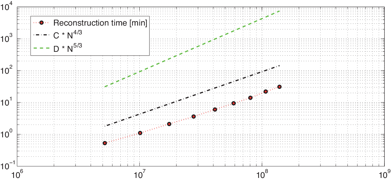
Figure 4.1: Log-log plot of the actual reconstruction time 𝚃⁡(𝙽)\tt{T}({\tt N}) of our Matlab implementation using (5) in dependence of the number of unknowns for 𝙽x=100,125,…,300{\tt N}_{x}=100,125,\dots,300. A comparison with the slopes of the log-log plots of 𝙲∗𝙽𝟺/𝟹\tt{C}*{\tt N}^{4/3} and 𝙳∗𝙽𝟻/𝟹\tt{D}*{\tt N}^{5/3} demonstrates the theoretical behavior 𝚃⁡(𝙽)=𝒪⁡(𝙽𝟺/𝟹)\tt{T}({\tt N})=\mathcal{O}({\tt N}^{4/3}). The constants 𝙲\tt{C}, 𝙳\tt{D} have been selected in simply in such a manner, that the above curves do not interfere with each other.

The partial backprojection operators are two-dimensional discrete backprojections for fixed 𝚔{\tt k} and 𝚗3{\tt n}_{3}, respectively. Assuming 𝙺,𝙻,𝙼=𝒪⁡(𝙽x){\tt K},{\tt L},{\tt M}=\mathcal{O}({\tt N}_{x}), both of these back-projection operators can be implemented using 𝒪⁡(𝙽x3)\mathcal{O}({\tt N}_{x}^{3}) floating point operations (see [32, 12]). Therefore, the numerical effort of evaluating (5) or (6) is 𝒪⁡(𝙽4/3)\mathcal{O}({\tt N}^{4/3}), where 𝙽=(2​𝙽x+1)2​(𝙻+1){\tt N}=(2{\tt N}_{x}+1)^{2}({\tt L}+1) is the total number of unknowns. Note that the direct implementation of a standard 3D spherical back-projection operator requires 𝒪⁡(𝙽5/3)\mathcal{O}({\tt N}^{5/3}) floating point operations, see [32, 33, 34]. Typically we have 𝙽x≥100{\tt N}_{x}\geq 100, and therefore our implementations are faster than the standard 3D spherical back-projections by at least two orders of magnitude. Figure 4.1 shows a log-log plot of the reconstruction time using (5) for 𝙽x∈{100,125,…,300}{\tt N}_{x}\in\{100,125,\dots,300\} (where we have chosen 𝙺,𝙻{\tt K},{\tt L}, and 𝙼{\tt M} proportional to 𝙽x{\tt N}_{x}) verifying that the number of floating point operations is 𝒪⁡(𝙽4/3)\mathcal{O}({\tt N}^{4/3}). For comparison purpose, Figure 4.1 also shows log-log plots of 𝙽↦𝙲∗𝙽𝟺/𝟹{\tt N}\mapsto\tt{C}*{\tt N}^{4/3} and 𝙽↦𝙳∗𝙽𝟻/𝟹{\tt N}\mapsto\tt{D}*{\tt N}^{5/3} for some constants 𝙲\tt{C}, 𝙳\tt{D}.

Refer to caption
Refer to caption
Refer to caption
Refer to caption
Refer to caption
Refer to caption
Figure 4.2: Reconstruction results using simulated data. Top row (from left to right): Horizontal slices of the phantom, the reconstruction using (5), and the reconstruction with the UBP (6). Bottom row: The same for the vertical slices.

4.2 Numerical results

For the numerical simulations presented below we consider superpositions of radially symmetric indicator functions. Figure 4.2 shows the considered phantom and the numerical reconstruction using the inversion formulas (5) and (6) for a1=1a_{1}=1, a2=0.8a_{2}=0.8, H=2H=2 and r0=4r_{0}=4. For the discretization we used 𝙺=256{\tt K}=256, 𝙻=200{\tt L}=200, 𝙼=400{\tt M}=400, and 𝙽x=100{\tt N}_{x}=100. In particular, the step size H/𝙻=0.01H/{\tt L}=0.01 in the vertical direction is chosen equal to the step size a1/𝙽x=0.01a_{1}/{\tt N}_{x}=0.01 in the horizontal direction and also to the radial step size r0/𝙼=0.01r_{0}/{\tt M}=0.01. We thereby use approximately five times more data points than unknowns, which mainly accounts for the fact that the detector elements cover a larger area than the reconstruction volume; while the step sizes are the same. Reducing the number of data points would introduce artifacts due to spatial undersampling; see [35]. One can see that the reconstruction results for all inversion formulas are very good, especially in the horizontal direction. In the vertical slice the vertical boundaries of the reconstructed balls are blurred. Such artifacts are expected and arise from truncating the observation surface, see [36, 37, 38, 39, 4, 40]. All computations have been performed in Matlab. The three dimensional reconstructed data sets consisting of (2​𝙽x2+1)​(𝙻+1)=8 120 601(2{\tt N}_{x}^{2}+1)({\tt L}+1)=8\,120\,601 unknowns and 𝙺​(2​𝙻+1)​(𝙼+1)=41 165 056{\tt K}(2{\tt L}+1)({\tt M}+1)=41\,165\,056 data points using either (5) or (6) have been computed in 6 minutes on a MacBook Pro with 2.3​GHz2.3\,\mathrm{GHz} Intel Core i7 processor.

Refer to caption
Refer to caption
Refer to caption
Refer to caption
Figure 4.3: Reconstruction results using noisy data. From left to right: Horizontal slice using (5), horizontal slice using (6), vertical slice using (5), and vertical slice using (6).

In order to illustrate the stability of the derived discrete back-projection algorithms with respect to the noise we applied all algorithms to simulated data, where we added Gaussian white noise with variance equal to 2%2\% of the maximal absolute value of 𝚐{\tt g}. The reconstruction results (using a1=1a_{1}=1, a2=0.8a_{2}=0.8, r0=4r_{0}=4, H=2H=2, 𝙺=256{\tt K}=256, 𝙻=200{\tt L}=200, 𝙼=400{\tt M}=400, and 𝙽x=100{\tt N}_{x}=100 as above) for noisy data are shown in Figure 4.3. As can be seen the implementations of all back-projection formulas perform quite stably with respect to noise. The slight amplification of noise is expected due to the ill-posedness of the inversion of the spherical Radon transform reflected by the two derivatives in any of the inversion formulas. The sensitivity with respect to noise could easily be further reduced by applying a regularization strategy similar to [34, 41] for the spherical Radon transform with centers on a sphere.

5 Conclusion

In this paper we studied an inversion of the spherical Radon transform in the case where the centers of the spheres of integration are located on a cylindrical surface Γ×ℝm\Gamma\times\mathbb{R}^{m}. We showed that this particular instance of the spherical Radon transform can be decomposed into two lower dimensional partial spherical Radon transforms, one with a center-set Γ⊆ℝn\Gamma\subseteq\mathbb{R}^{n} and one with a planar center-set in ℝm+1\mathbb{R}^{m+1}, see Theorem 2.3. This factorization was used to derive explicit inversion formulas for elliptical and circular cylinders. We emphasize, that our factorization approach can also be used for more general cylinders in combination with existing algorithms for an inversion from spherical means on bounded domains, such as time reversal or series expansion.

Appendix A Proof of explicit inversion formulas

A.1 Proof of Theorem 3.1

In this appendix we derive the inversion formula (2) stated in Theorem 3.1. For that purpose we first give an inversion formula for spherical means on an ellipsoid that essentially follows from [19, 22].

Lemma A.1.

For f∈Cc∞​(EA×ℝm)f\in C_{c}^{\infty}(E_{A}\times\mathbb{R}^{m}) and every (x,y)∈EA×ℝm(x,y)\in E_{A}\times\mathbb{R}^{m}, we have

f⁡(x,y)=2n−3​det(A)|𝕊n−2|​(n−2)!​(ΔA​x​𝐌x♯​𝐂s​𝐌x​f)​(x,y),f\left(x,y\right)=\frac{2^{n-3}\det(A)}{\lvert\mathbb{S}^{n-2}\rvert(n-2)!}\left(\Delta_{Ax}\mathbf{M}_{x}^{\sharp}\mathbf{C}_{s}\mathbf{M}_{x}f\right)\left(x,y\right)\,, (7)

with

(𝐂s​h)​(x,y,s)≔{2π​∫0∞s′​h​(x,y,s′)​log⁡|s2−s′2|​ds′n=2,(−1)(n−1)/2​(s​𝐃sn−3​sn−2​h)​(x,y,s)n≥3 odd,(−1)(n−2)/2​(𝐇s​𝐃sn−3​sn−2​h)​(x,y,s)n≥4 even.(\mathbf{C}_{s}h)\left(x,y,s\right)\coloneqq\begin{cases}\frac{2}{\pi}\int_{0}^{\infty}s^{\prime}h\left(x,y,s^{\prime}\right)\log\left\lvert s^{2}-s^{\prime 2}\right\rvert\ds^{\prime}&\text{$n=2,$}\\ (-1)^{(n-1)/2}\left(s\mathbf{D}_{s}^{n-3}s^{n-2}h\right)\left(x,y,s\right)&\text{$n\geq 3$ odd}\,,\\ (-1)^{(n-2)/2}\left(\mathbf{H}_{s}\mathbf{D}_{s}^{n-3}s^{n-2}h\right)\left(x,y,s\right)&\text{$n\geq 4$ even}\,.\end{cases}
Proof.

For n=2n=2 and n=3n=3, the inversion formula (7) has been derived in [22] and for odd n≥3n\geq 3 in [19]. For even n≥4n\geq 4, in [19] the following inversion formula has been shown:

f⁡(x,y)=2n−3​det(A)|𝕊n−2|​(n−2)!​(−1)(n−2)/2​ΔA​x​∫Sn−12π​∫0∞(𝐃sn−2​sn−2​𝐌x​f)​(A​σ,y,s)​log⁡||x−A​σ|2−s2|​s​ds​dS⁡(σ).f\left(x,y\right)=\frac{2^{n-3}\det(A)}{\lvert\mathbb{S}^{n-2}\rvert(n-2)!}(-1)^{(n-2)/2}\Delta_{Ax}\int_{S^{n-1}}\frac{2}{\pi}\int_{0}^{\infty}\left(\mathbf{D}_{s}^{n-2}s^{n-2}\mathbf{M}_{x}f\right)\left(A\sigma,y,s\right)\log\left\lvert|x-A\sigma|^{2}-s^{2}\right\rvert s\ds\dS(\sigma)\,. (8)

Using 2​s​(s2−|A​σ−x|2)−1=(s−|A​σ−x|)−1+(s+|A​σ−x|)−12s(s^{2}-|A\sigma-x|^{2})^{-1}=(s-|A\sigma-x|)^{-1}+(s+|A\sigma-x|)^{-1}, the inner integral in (8) can be written as

2π​∫0∞(𝐃sn−2​sn−2​𝐌x​f)​(A​σ,y,s)​log⁡||x−A​σ|2−s2|​s​ds=1π​P.V.∫0∞(𝐃sn−3​sn−2​𝐌x​f)​(A​σ,y,s)​2​s​dss2−|x−A​σ|2=1π[P.V.∫0∞(𝐃sn−3​sn−2​𝐌x​f)​(A​σ,y,s)s−|x−A​σ|ds+∫0∞(𝐃sn−3​sn−2​𝐌x​f)​(A​σ,y,s)s+|x−A​σ|ds]=1π​P.V.∫ℝ(𝐃sn−3​sn−2​𝐌x​f)​(A​σ,y,s)s−|x−A​σ|​ds=(𝐇s​𝐃sn−3​sn−2​𝐌x​f)​(A​σ,y,|x−A​σ|).\frac{2}{\pi}\int_{0}^{\infty}\left(\mathbf{D}_{s}^{n-2}s^{n-2}\mathbf{M}_{x}f\right)\left(A\sigma,y,s\right)\log\left\lvert|x-A\sigma|^{2}-s^{2}\right\rvert s\ds\\ \begin{aligned} &=\frac{1}{\pi}\,\mathrm{P.V.}\!\int_{0}^{\infty}\left(\mathbf{D}_{s}^{n-3}s^{n-2}\mathbf{M}_{x}f\right)\left(A\sigma,y,s\right)\frac{2s\ds}{s^{2}-|x-A\sigma|^{2}}\\ &=\frac{1}{\pi}\left[\,\mathrm{P.V.}\!\int_{0}^{\infty}\frac{\left(\mathbf{D}_{s}^{n-3}s^{n-2}\mathbf{M}_{x}f\right)\left(A\sigma,y,s\right)}{s-|x-A\sigma|}\ds+\int_{0}^{\infty}\frac{\left(\mathbf{D}_{s}^{n-3}s^{n-2}\mathbf{M}_{x}f\right)\left(A\sigma,y,s\right)}{s+|x-A\sigma|}\ds\right]\\ &=\frac{1}{\pi}\,\mathrm{P.V.}\!\int_{\mathbb{R}}\frac{\left(\mathbf{D}_{s}^{n-3}s^{n-2}\mathbf{M}_{x}f\right)\left(A\sigma,y,s\right)}{s-|x-A\sigma|}\ds\\ &=\left(\mathbf{H}_{s}\mathbf{D}_{s}^{n-3}s^{n-2}\mathbf{M}_{x}f\right)\left(A\sigma,y,|x-A\sigma|\right)\,.\end{aligned}

Inserting the last displayed equation in (8) shows (7) for the case of even n≥4n\geq 4. ∎

Lemma A.2.

For even and differentiable h:ℝ→ℝh\colon\mathbb{R}\to\mathbb{R} we have 𝐇s​𝐃s​𝐇s​h=−𝐃s​h\mathbf{H}_{s}\mathbf{D}_{s}\mathbf{H}_{s}h=-\mathbf{D}_{s}h.

Proof.

Since hh is even, 𝐇s​h\mathbf{H}_{s}h and 𝐃s​𝐇s​h\mathbf{D}_{s}\mathbf{H}_{s}h are odd in ss. Now, for any odd function φ:ℝ→ℝ\varphi\colon\mathbb{R}\to\mathbb{R}, we get

(𝐇sφ)(s)=1πP.V.∫ℝφ⁡(s′)s−s′ds′=1π(P.V.∫0∞φ⁡(s′)s−s′ds′−P.V.∫0∞φ⁡(s′)s+s′ds′)=1π​P.V.∫0∞2​s′s2−(s′)2​φ​(s′)​ds′.(\mathbf{H}_{s}\varphi)(s)=\frac{1}{\pi}\,\mathrm{P.V.}\!\int_{\mathbb{R}}\frac{\varphi(s^{\prime})}{s-s^{\prime}}\ds^{\prime}=\frac{1}{\pi}\left(\mathrm{P.V.}\!\int_{0}^{\infty}\frac{\varphi(s^{\prime})}{s-s^{\prime}}\ds^{\prime}-\mathrm{P.V.}\!\int_{0}^{\infty}\frac{\varphi(s^{\prime})}{s+s^{\prime}}\ds^{\prime}\right)\\ =\frac{1}{\pi}\,\mathrm{P.V.}\!\int_{0}^{\infty}\frac{2s^{\prime}}{s^{2}-(s^{\prime})^{2}}\varphi(s^{\prime})\ds^{\prime}\,. (9)

Applying (9) once with φ=𝐃s​𝐇s​h\varphi=\mathbf{D}_{s}\mathbf{H}_{s}h and once with φ=𝐇s​h\varphi=\mathbf{H}_{s}h yields

(𝐇s​𝐃s​𝐇s​h)​(s)\displaystyle(\mathbf{H}_{s}\mathbf{D}_{s}\mathbf{H}_{s}h)(s) =1π​P.V.∫0∞2​s′s2−(s′)2​(𝐃s​𝐇s​h)​(s′)​ds′\displaystyle=\frac{1}{\pi}\,\mathrm{P.V.}\!\int_{0}^{\infty}\frac{2s^{\prime}}{s^{2}-(s^{\prime})^{2}}(\mathbf{D}_{s}\mathbf{H}_{s}h)(s^{\prime})\ds^{\prime}
=𝐃s​1π​P.V.∫0∞2​s′s2−(s′)2​(𝐇s​h)​(s′)​ds′=(𝐃s​𝐇s​𝐇s​h)​(s)=−𝐃s​h​(s).∎\displaystyle=\mathbf{D}_{s}\,\frac{1}{\pi}\,\mathrm{P.V.}\!\int_{0}^{\infty}\frac{2s^{\prime}}{s^{2}-(s^{\prime})^{2}}(\mathbf{H}_{s}h)(s^{\prime})\ds^{\prime}=(\mathbf{D}_{s}\mathbf{H}_{s}\mathbf{H}_{s}h)(s)=-\mathbf{D}_{s}h(s)\,.\qed

Now we are ready to prove Theorem 3.1. For that purpose, let f∈Cc∞​(EA×ℝm)f\in C_{c}^{\infty}(E_{A}\times\mathbb{R}^{m}). From Theorem 2.3 and the inversion formula [6] for the spherical Radon transform with a planar center-set (see also [10, 9]), we obtain

𝐌x​f=|𝕊n+m−1|(2​π)m​|𝕊n−1|​(|s|1−n​(−Δy,s)(m−1)/2​𝐇s​∂s𝐌y,s♯​|r|n−1​𝐌x,y​f).\mathbf{M}_{x}f=\frac{\lvert\mathbb{S}^{{n+m}-1}\rvert}{(2\pi)^{m}\lvert\mathbb{S}^{n-1}\rvert}\Bigl(\left\lvert s\right\rvert^{1-n}(-\Delta_{y,s})^{(m-1)/2}\mathbf{H}_{s}\partial_{s}\mathbf{M}_{y,s}^{\sharp}\left\lvert r\right\rvert^{n-1}\mathbf{M}_{x,y}f\Bigr)\,. (10)

Together with (7) this gives

f⁡(x,y)\displaystyle f(x,y) =2n−3​det(A)|𝕊n−2|​(n−2)!​(ΔA​x​𝐌x♯​𝐂s​𝐌x​f)​(x,y)\displaystyle=\frac{2^{n-3}\det(A)}{\lvert\mathbb{S}^{n-2}\rvert(n-2)!}\left(\Delta_{Ax}\mathbf{M}_{x}^{\sharp}\mathbf{C}_{s}\mathbf{M}_{x}f\right)(x,y)
=2n−3​det(A)|𝕊n−2|​(n−2)!​|𝕊n+m−1|(2​π)m​|𝕊n−1|​(ΔA​x​𝐌x♯​𝐂s​|s|1−n​(−Δy,s)(m−1)/2​𝐇s​∂s𝐌y,s♯​|r|n−1​𝐌x,y​f)​(x,y)\displaystyle=\frac{2^{n-3}\det(A)}{\lvert\mathbb{S}^{n-2}\rvert(n-2)!}\frac{\lvert\mathbb{S}^{{n+m}-1}\rvert}{(2\pi)^{m}\lvert\mathbb{S}^{n-1}\rvert}\left(\Delta_{Ax}\mathbf{M}_{x}^{\sharp}\mathbf{C}_{s}\left\lvert s\right\rvert^{1-n}(-\Delta_{y,s})^{(m-1)/2}\mathbf{H}_{s}\partial_{s}\mathbf{M}_{y,s}^{\sharp}\left\lvert r\right\rvert^{n-1}\mathbf{M}_{x,y}f\right)(x,y)
=2n−2​det(A)(2​π)m​(n−2)!​|𝕊n+m−1||𝕊n−2|​|𝕊n−1|​(ΔA​x​𝐌x♯​𝐁s​(−Δy,s)(m−1)/2​𝐌y,s♯​|r|n−1​𝐌x,y​f)​(x,y),\displaystyle=\frac{2^{n-2}\det(A)}{(2\pi)^{m}(n-2)!}\frac{\lvert\mathbb{S}^{{n+m}-1}\rvert}{\lvert\mathbb{S}^{n-2}\rvert\lvert\mathbb{S}^{n-1}\rvert}\left(\Delta_{Ax}\mathbf{M}_{x}^{\sharp}\mathbf{B}_{s}(-\Delta_{y,s})^{(m-1)/2}\mathbf{M}_{y,s}^{\sharp}\left\lvert r\right\rvert^{n-1}\mathbf{M}_{x,y}f\right)(x,y)\,,

with

(𝐁s​h)​(x,y,s)={1π​∫0∞(∂s𝐇s​h)​(x,y,s′)​log⁡|s2−s′2|​ds′if n=2,12​(−1)(n−1)/2​(s​𝐃sn−3​s−1​∂s𝐇s​h)​(x,y,s)if n≥3 odd,12​(−1)(n−2)/2​(𝐇s​𝐃sn−3​s−1​∂s𝐇s​h)​(x,y,s)if n≥4 even.(\mathbf{B}_{s}h)\left(x,y,s\right)=\begin{cases}\frac{1}{\pi}\int_{0}^{\infty}(\partial_{s}\mathbf{H}_{s}h)\left(x,y,s^{\prime}\right)\log\left\lvert s^{2}-s^{\prime 2}\right\rvert\ds^{\prime}&\text{if $n=2$,}\\ \frac{1}{2}(-1)^{(n-1)/2}\left(s\mathbf{D}_{s}^{n-3}s^{-1}\partial_{s}\mathbf{H}_{s}h\right)\left(x,y,s\right)&\text{if $n\geq 3$ odd,}\\ \frac{1}{2}(-1)^{(n-2)/2}\left(\mathbf{H}_{s}\mathbf{D}_{s}^{n-3}s^{-1}\partial_{s}\mathbf{H}_{s}h\right)\left(x,y,s\right)&\text{if $n\geq 4$ even}\,.\end{cases}

It remains to verify, that 𝐁\mathbf{B} can be written in the form (3). For n≥3n\geq 3 odd this follows from 𝐃s=1/2s−1∂s\mathbf{D}_{s}=1/2s^{-1}\partial_{s}. In the case n=2n=2 integration by parts and applying (9) shows

(𝐁s​h)​(x,y,s)\displaystyle(\mathbf{B}_{s}h)\left(x,y,s\right) =−1π​P.V.∫0∞(𝐇s​h)​(x,y,s′)​2​s′s2−s′2​ds′=−(𝐇s​𝐇s​h)​(x,y,s)=h⁡(x,y,s).\displaystyle=-\frac{1}{\pi}\,\mathrm{P.V.}\!\int_{0}^{\infty}(\mathbf{H}_{s}h)\left(x,y,s^{\prime}\right)\frac{2s^{\prime}}{s^{2}-s^{\prime 2}}\ds^{\prime}=-(\mathbf{H}_{s}\mathbf{H}_{s}h)\left(x,y,s\right)=h\left(x,y,s\right)\,.

Finally, for the case that n≥4n\geq 4, repeated application of Lemma A.2 implies that 𝐁\mathbf{B} is given by (3), and concludes the proof.

A.2 Proof of Theorem 3.2

To prove Theorem 3.2 we use the following modification of one of the formulas of [12, Corollary 1.2].

Lemma A.3.

For f∈Cc∞​(DR×ℝm)f\in C_{c}^{\infty}(D_{R}\times\mathbb{R}^{m}) and (x,y)∈DR×ℝm(x,y)\in D_{R}\times\mathbb{R}^{m}, we have

f⁡(x,y)=12​(𝐌x♯​𝐇s​∂s|s|​𝐌x​f)​(x,y).f(x,y)=\frac{1}{2}\left(\mathbf{M}_{x}^{\sharp}\mathbf{H}_{s}\partial_{s}\left\lvert s\right\rvert\mathbf{M}_{x}f\right)(x,y)\,. (11)
Proof.

The proof is based on [12] and a range condition for 𝐌x\mathbf{M}_{x} derived in [42]. The range condition for the spherical Radon transform of [42] yields

0\displaystyle 0 =∫∂DRP.V.∫0∞2​ss2−|x′−x|2​𝐌x​f​(x′,y,s)​ds⁡dS⁡(x′)\displaystyle=\int_{\partial D_{R}}\mathrm{P.V.}\!\int_{0}^{\infty}\frac{2s}{s^{2}-|x^{\prime}-x|^{2}}\mathbf{M}_{x}f(x^{\prime},y,s)\ds\dS(x^{\prime})
=∫∂DRP.V.∫0∞𝐌x​f​(x′,y,s)​ds⁡dS⁡(x′)s−|x′−x|+∫∂DR∫0∞𝐌x​f​(x′,y,s)​ds⁡dS⁡(x′)s+|x′−x|\displaystyle=\int_{\partial D_{R}}\mathrm{P.V.}\!\int_{0}^{\infty}\mathbf{M}_{x}f(x^{\prime},y,s)\frac{\ds\dS(x^{\prime})}{s-|x^{\prime}-x|}+\int_{\partial D_{R}}\int_{0}^{\infty}\mathbf{M}_{x}f(x^{\prime},y,s)\frac{\ds\dS(x^{\prime})}{s+|x^{\prime}-x|}
=∫∂DRP.V.∫ℝsign⁡(s)​𝐌x​f​(x′,y,s)​ds⁡dS⁡(x′)s−|x′−x|\displaystyle=\int_{\partial D_{R}}\mathrm{P.V.}\!\int_{\mathbb{R}}\operatorname{sign}(s)\mathbf{M}_{x}f(x^{\prime},y,s)\frac{\ds\dS(x^{\prime})}{s-|x^{\prime}-x|}
=(𝐌x♯​𝐇s​sign⁡(s)​𝐌x​f)​(x,y).\displaystyle=\left(\mathbf{M}_{x}^{\sharp}\mathbf{H}_{s}\operatorname{sign}(s)\mathbf{M}_{x}f\right)(x,y)\,. (12)

By the product rule, we have

(𝐌x♯​𝐇s​∂s|s|​𝐌x​f)​(x,y)=(𝐌x♯​𝐇s​sign⁡(s)​𝐌x​f)​(x,y)+(𝐌x♯​𝐇s​|s|​∂s𝐌x​f)​(x,y).\left(\mathbf{M}_{x}^{\sharp}\mathbf{H}_{s}\partial_{s}\left\lvert s\right\rvert\mathbf{M}_{x}f\right)(x,y)=\left(\mathbf{M}_{x}^{\sharp}\mathbf{H}_{s}\operatorname{sign}(s)\mathbf{M}_{x}f\right)(x,y)+\left(\mathbf{M}_{x}^{\sharp}\mathbf{H}_{s}\left\lvert s\right\rvert\partial_{s}\mathbf{M}_{x}f\right)(x,y)\,.

According to (12), the first term in the last displayed equation equals zero, and according to [12, Eq. (1.6)] the second term is equal to 2​f​(x,y)2f(x,y). This completes the proof. ∎

The inversion formula (4) now follows from (10) and (11). In fact,

f⁡(x,y)\displaystyle f(x,y) =12​(𝐌x♯​𝐇s​∂s|s|​𝐌x​f)​(x,y)\displaystyle=\frac{1}{2}\left(\mathbf{M}_{x}^{\sharp}\mathbf{H}_{s}\partial_{s}\left\lvert s\right\rvert\mathbf{M}_{x}f\right)(x,y)
=|𝕊m+1|2​(2​π)m+1​(𝐌x♯​𝐇s​∂s(−Δy,s)(m−1)/2​𝐇s​∂s𝐌y,s♯​|r|​𝐌x,y​f)​(x,y)\displaystyle=\frac{\lvert\mathbb{S}^{m+1}\rvert}{2(2\pi)^{m+1}}\left(\mathbf{M}_{x}^{\sharp}\mathbf{H}_{s}\partial_{s}(-\Delta_{y,s})^{(m-1)/2}\mathbf{H}_{s}\partial_{s}\mathbf{M}_{y,s}^{\sharp}\left\lvert r\right\rvert\mathbf{M}_{x,y}f\right)(x,y)
=−|𝕊m+1|2​(2​π)m+1​(𝐌x♯​(−Δy,s)(m−1)/2​∂s2𝐌y,s♯​|r|​𝐌x,y​f)​(x,y),\displaystyle=-\frac{\lvert\mathbb{S}^{m+1}\rvert}{2(2\pi)^{m+1}}\left(\mathbf{M}_{x}^{\sharp}(-\Delta_{y,s})^{(m-1)/2}\partial_{s}^{2}\mathbf{M}_{y,s}^{\sharp}\left\lvert r\right\rvert\mathbf{M}_{x,y}f\right)(x,y)\,,

where we used two identities 𝐇s​∂s(−Δy,s)(m−1)/2=(−Δy,s)(m−1)/2​∂s𝐇s\mathbf{H}_{s}\partial_{s}(-\Delta_{y,s})^{(m-1)/2}=(-\Delta_{y,s})^{(m-1)/2}\partial_{s}\mathbf{H}_{s} and 𝐇s​𝐇s​h=−h\mathbf{H}_{s}\mathbf{H}_{s}h=-h.

Acknowledgements

The work of the second author was supported in part by the National Research Foundation of Korea (NRF) grant funded by the Korea government (MSIP) (No.2015R1C1A1A01051674) and supported by the TJ Park Science Fellowship of POSCO TJ Park Foundation.

Bibliography

References

  • Kruger et al. [1995] R. A. Kruger, P. Liu, Y. R. Fang, C. R. Appledorn, Photoacoustic ultrasound (PAUS)–Reconstruction tomography, Med. Phys. 22 (10) (1995) 1605–1609.
  • Wang [2009] L. V. Wang, Photoacoustic Imaging and Spectroscopy, Optical Science and Engineering, Taylor & Francis, ISBN 9781420059922, 2009.
  • Hellsten and Andersson [1987] H. Hellsten, L. E. Andersson, An inverse method for the processing of synthetic aperture RADAR data, Inverse Probl. 3 (1) (1987) 111–124.
  • Stefanov and Uhlmann [2013] P. Stefanov, G. Uhlmann, Is a curved flight path in SAR better than a straight one?, SIAM J. Appl. Math. 73 (4) (2013) 1596–1612.
  • Norton and Norton [1981] S. J. Norton, S. Norton, Ultrasonic reflectivity imaging in three dimensions: exact inverse scattering solutions for plane, cylindrical, and spherical apertures, IEEE Trans. Biomed. Eng. BME-28 (2) (1981) 202–220.
  • Andersson [1988] L. Andersson, On the determination of a function from spherical averages, SIAM J. Math. Anal. 19 (1) (1988) 214–232.
  • Beltukov [2009] A. Beltukov, Inversion of the Spherical Mean Transform with Sources on a Hyperplane, arXiv:0919.1380v1, 2009.
  • Buhgeim and Kardakov [1978] A. L. Buhgeim, V. B. Kardakov, Solution of an inverse problem for an elastic wave equation by the method of spherical means, Sibirsk. Mat. Z. 19 (4) (1978) 749–758.
  • Fawcett [1985] J. Fawcett, Inversion of nn-dimensional spherical averages, SIAM J. Appl. Math. 45 (2) (1985) 336–341.
  • Klein [2003] J. Klein, Inverting the spherical Radon transform for physically meaningful functions, 2003.
  • Narayanan and Rakesh [2010] E. K. Narayanan, Rakesh, Spherical means with centers on a hyperplane in even dimensions, Inverse Probl. 26 (3) (2010) 035014.
  • Finch et al. [2007] D. Finch, M. Haltmeier, Rakesh, Inversion of spherical means and the wave equation in even dimensions, SIAM J. Appl. Math. 68 (2007) 392–412.
  • Finch et al. [2004] D. Finch, S. Patch, Rakesh, Determining a function from its mean values over a family of spheres, SIAM J. Math. Anal. 35 (5) (2004) 1213–1240.
  • Kunyansky [2007a] L. A. Kunyansky, Explicit inversion formulae for the spherical mean Radon transform, Inverse Probl. 23 (1) (2007a) 373–383.
  • Nguyen [2009] L. V. Nguyen, A family of inversion formulas for thermoacoustic tomography, Inverse Probl. Imaging 3 (4) (2009) 649–675.
  • Xu and Wang [2005] M. Xu, L. Wang, Universal back-projection algorithm for photoacoustic computed tomography, Phys. Rev. E 71 (1) (2005) 016706.
  • Ansorg et al. [2013] M. Ansorg, F. Filbir, W. R. Madych, R. Seyfried, Summability kernels for circular and spherical mean data, Inverse Probl. 29 (1) (2013) 015002.
  • Haltmeier [2014a] M. Haltmeier, Universal inversion formulas for recovering a function from spherical means, SIAM J. Math. Anal. 46 (1) (2014a) 214–232.
  • Haltmeier [2014b] M. Haltmeier, Exact reconstruction formula for the spherical mean radon transform on ellipsoids, Inverse Probl. 30 (10) (2014b) 105006.
  • Natterer [2012] F. Natterer, Photo-acoustic inversion in convex domains, Inverse Probl. Imaging 6 (2) (2012) 315–320.
  • Palamodov [2012] V. P. Palamodov, A uniform reconstruction formula in integral geometry, Inverse Probl. 28 (6) (2012) 065014.
  • Salman [2014] Y. Salman, An inversion formula for the spherical mean transform with data on an ellipsoid in two and three dimensions, J. Math. Anal. Appl. 420 (2014) 612–620.
  • Haltmeier and Pereverzyev [2015a] M. Haltmeier, S. Pereverzyev, Jr., Recovering a function from circular means or wave data on the boundary of parabolic domains, SIAM J. Imaging Sci. 8 (1) (2015a) 592–610.
  • Haltmeier and Pereverzyev [2015b] M. Haltmeier, S. Pereverzyev, Jr., The universal back-projection formula for spherical means and the wave equation on certain quadric hypersurfaces, J. Math. Anal. Appl. 429 (1) (2015b) 366–382.
  • Palamodov [2014] V. P. Palamodov, Time reversal in photoacoustic tomography and levitation in a cavity, Inverse Probl. 30 (12) (2014) 125006 (16 pages).
  • Kunyansky [2015] L. Kunyansky, Inversion of the spherical means transform in corner-like domains by reduction to the classical Radon transform, Inverse Probl. 31 (095001).
  • Burgholzer et al. [2007a] P. Burgholzer, G. J. Matt, M. Haltmeier, G. Paltauf, Exact and approximate imaging methods for photoacoustic tomography using an arbitrary detection surface, Phys. Rev. E 75 (2007a) 046706.
  • Hristova et al. [2008] Y. Hristova, P. Kuchment, L. Nguyen, Reconstruction and time reversal in thermoacoustic tomography in acoustically homogeneous and inhomogeneous media, Inverse Probl. 24 (5) (2008) 055006 (25pp).
  • Treeby and Cox [2010] B. E. Treeby, B. T. Cox, k-Wave: MATLAB toolbox for the simulation and reconstruction of photoacoustic wave-fields, J. Biomed. Opt. 15 (2010) 021314.
  • Agranovsky and Kuchment [2007] M. Agranovsky, P. Kuchment, Uniqueness of reconstruction and an inversion procedure for thermoacoustic and photoacoustic tomography with variable sound speed, Inverse Probl. 23 (5) (2007) 2089–2102.
  • Kunyansky [2007b] L. A. Kunyansky, A series solution and a fast algorithm for the inversion of the spherical mean Radon transform, Inverse Probl. 23 (6) (2007b) S11–S20.
  • Burgholzer et al. [2007b] P. Burgholzer, J. Bauer-Marschallinger, H. Grün, M. Haltmeier, G. Paltauf, Temporal back-projection algorithms for photoacoustic tomography with integrating line detectors, Inverse Probl. 23 (6) (2007b) S62–S80.
  • Kunyansky [2012] L. A. Kunyansky, Fast reconstruction algorithms for the thermoacoustic tomography in certain domains with cylindrical or spherical symmetries, Inverse Probl. Imaging 6 (1) (2012) 111–131.
  • Haltmeier et al. [2005] M. Haltmeier, T. Schuster, O. Scherzer, Filtered backprojection for thermoacoustic computed tomography in spherical geometry, Math. Methods Appl. Sci. 28 (16) (2005) 1919–1937, ISSN 0170-4214.
  • Haltmeier [2016] M. Haltmeier, Sampling conditions for the circular Radon transform, IEEE Trans. Image Process. 25 (6) (2016) 2910–2919.
  • Frikel and Quinto [2015] J. Frikel, E. T. Quinto, Artifacts in incomplete data tomography with applications to photoacoustic tomography and sonar, SIAM J. Appl. Math. 75 (2) (2015) 703–725.
  • Kunyansky [2008] L. A. Kunyansky, Thermoacoustic tomography with detectors on an open curve: an efficient reconstruction algorithm, Inverse Probl. 24 (5) (2008) 055021.
  • Nguyen [2015] L. V. Nguyen, On artifacts in limited data spherical radon transform: flat observation surfaces, SIAM J. Math. Anal. 47 (4) (2015) 2984–3004.
  • Paltauf et al. [2007] G. Paltauf, R. Nuster, M. Haltmeier, P. Burgholzer, Experimental evaluation of reconstruction algorithms for limited view photoacoustic tomography with line detectors, Inverse Probl. 23 (6) (2007) S81–S94.
  • Xu et al. [2004] Y. Xu, L. V. Wang, G. Ambartsoumian, P. Kuchment, Reconstructions in limited-view thermoacoustic tomography, Med. Phys. 31 (4) (2004) 724–733.
  • Haltmeier [2011] M. Haltmeier, A mollification approach for inverting the spherical mean Radon transform, SIAM J. Appl. Math. 71 (5) (2011) 1637–1652.
  • Finch and Rakesh [2009] D. Finch, Rakesh, Recovering a function from its spherical mean values in two and three dimensions, in: L. Wang (Ed.), Photoacoustic Imaging and Spectroscopy, Optical Science and Engineering, Taylor & Francis, 2009.