Direct reconstruction of dynamical dark energy from observational Hubble parameter data Note: Fully documented templates are available in the elsarticle package on CTAN.
Abstract
Reconstructing the evolution history of the dark energy equation of state parameter directly from observational data is highly valuable in cosmology, since it contains substantial clues in understanding the nature of the accelerated expansion of the Universe. Many works have focused on reconstructing using Type Ia supernova data, however, only a few studies pay attention to Hubble parameter data. In the present work, we explore the merit of Hubble parameter data and make an attempt to reconstruct from them through the principle component analysis approach. We find that current Hubble parameter data perform well in reconstructing ; though, when compared to supernova data, the data are scant and their quality is worse. Both CDM and evolving models can be constrained within at redshifts and even at redshifts 0.1 z 1 by using simulated data of observational quality.
Keywords:
Dark Energy , Reconstruction, Nonparametric Model , Observational Hubble Parameter Data1 Introduction
There have been a handful of works reconstructing the dark energy equation of state parameter , defined as , where and represent the pressure and energy density, from observed distance modulus data (e.g., Type Ia supernova (SN Ia) data). Basically, these works can be divided into two categories: (i) Assume a particular model about so that the model quantities (e.g., luminosity distance ) can be compared directly with the observations. (ii) Characterize the data with an underlying model and then reconstruct numerically. For category (i), the assumed model can be expressed as a parameterized form of a basis representation or a function distribution representation. The parametric forms are currently the most commonly used, which either assume is a constant or allow for a redshift dependence, such as , where and are constants [1, 2]. Hojjati et al. [3] used wavelets to study the redshift evolution of . In that work the Principal Component Analysis (PCA) technique, which has the advantage of detecting local features such as bumps in , was applied to decorrelate the wavelet coefficients. Huterer et al. [4] presented a piecewise constant description of by binning redshifts, and estimated the corresponding band power. The PCA was also used to make the band power uncorrelated so that the eigenmodes can be written as linear combinations of redshift bins. Holsclaw et al. [5] introduced a non-parametric reconstruction method by modeling through a Gaussian process (GP) and estimating the GP hyperparameters with a Bayesian inference and Markov chain Monte Carlo sampling. Zhao et al. [6] combined GP and redshift binning method to feature , in which the value in each bin is treated as free parameter to be determined. To make differentiable for the calculation of the dark energy perturbations, they interpolated between the bins with narrow tanh functions.For category (ii), Daly et al. [7] developed a simple numerical method to determine from the data, which made no assumptions about the underlying cosmological models. Their approach is model-independent. However, the final results are noisier and highly sensitive to the amount and quality of the available data. To suppress the noise, Shafieloo et al. [8] smoothed the SN Ia data by applying a Gaussian kernel over the whole redshift range before performing reconstruction. Majumdar et al. [9] expressed the distance modulus in a parametric form, , and used the standard minimization to determine the parameters (a, b, ). Clarkson et al. [10] fitted the data before reconstruction using eigenmodes which were transformed from a set of primal basis functions with PCA.
With observational data getting richer and more diverse, recently researchers have begun to study dark energy reconstruction with multiple sets of measurements. Holsclaw et al. [11] extended their Gaussian process method [5] to include a diverse set of measurements: baryon acoustic oscillations (BAO), cosmic microwave background measurements (CMB), and supernova data (SNe), while observational Hubble parameter data (OHD) were used by other researchers [9, 6, 12].
So far, most research has focused on observational data acquired from SNe, CMB, and BAO, especially from SNe, or their hypothetical counterparts. On the contrary, the problem of reconstructing dark energy from Hubble parameter data has attracted less attention of the cosmology community. How valuable are OHD in modeling the Universe? In fact, some pioneers have made explorative works in this area. Ma et al. [13] studied the viability of constraining the cosmological parameters using OHD and concluded that as many as 64 data points are sufficient to get a result comparative to SNe data. Pan et al. [14] discovered that to some extent the OHD were better poised to give information about the nature of dark energy than the SN Ia data. Encouraged by these pioneering works, in this paper we attempt to reconstruct dark energy solely with the help of OHD.
2 Merit of the Hubble parameter
Although, as previously mentioned, some authors have considered the role of OHD in reconstructing dark energy with combined data sets, few researchers have tried to use OHD solely to undertake this task [15]. This is partially due to the smaller number and lower quality of OHD compared to the distance module data. In contrast to the 580 SN Ia data released by the supernova cosmology project [16], to date, the most comprehensive sample of OHD contains only 37 measurements (see Figs. 1). They are collected from [17, 18, 19, 20, 21, 22, 23, 24, 15, 25], most of which are compiled in [26]. Current OHD are obtained primarily by the cosmic chronometers method (30 measurements) [17, 18, 20, 24, 15]. Radial BAO peaks detection is another method to extract [21, 22, 23]. The cosmic chronometers method is affected by the systematic biases in the age determination of galaxies, while for the radial BAO method, the systematics stem from various distortion effects subjected to the autocorrelation function. Since a fiducial flat Lambda cold dark matter (CDM) model and its parameters are used to convert redshifts into distances and to gauge the comoving BAO scales in the selected redshift slice [27], the radial BAO method is essentially model-dependent, and the possible circular logic issue also contributes to the systematic errors in this method [28]. Since OHD measurements coming from different techniques may suffer from different systematic effects, the 30 measurements that come from cosmic chronometers are adopted in our analysis (see Fig.1). They all have been compiled in Ref. [15].

OHD (with mean relative error of ) have generally larger error bars than SN Ia data (with mean relative error of merely ). However, OHD have more direct and efficient power to constrain compared to SN Ia data. is written in terms of as Equation (1) [10]:
| (1) | |||||
Here and are normalized density parameters of matter and curvature and prime denotes the derivative with respect to . is the normalized comoving distance and is the Hubble constant. Note that the second derivative of is a prerequisite in Eq. (1) even in the case of . We can decompose Eq. (1) into two simpler equations by introducing the Hubble parameter as the intermediate quantity, which can be expressed as Equation (2),
| (2) |
and Equation (3),
| (3) |
Eq. (3) shows that to calculate from , only the first derivative of is needed. The derivative operator functions as a high-pass filter and can thus heavily amplify the observational errors. Therefore, to reconstruct , is preferable to when regarding the suppression of the propagation of noise [29]. Such an advantage of makes it a promising method to reconstruct directly from instead of , although the current quality of data is comparatively poor. It should be noted that Pan et al. [14] have given an estimate about the advantage of the first derivative of data over the second derivative in reconstructing dark energy. They studied the efficacy of four different parameters: the deceleration parameter, the equation of state of dark energy, the dark energy density, and the geometrical parameters , which can be expressed as Equation (4) [30]:
| (4) |
In discriminating theoretical models of dark energy using supernova data, they found that the geometrical parameters , a cosmological parameter constructed from the first derivative of the data, for which the theoretical models of dark energy are sufficiently distant from each other, performs best in reconstructing dark energy from SNe data.
3 Methodology
Most existing reconstruction approaches making use of the observed distance modulus data can also be applied to OHD. Here we apply the framework of weighted least square (WLS) and PCA [10]. Given a set of data , we fit them with a smooth analytical function, and then use it and its first derivative to reconstruct according to Eq. (3). Assume the covariance matrix of the data satisfies for and for . We start with a set of N primary basis functions , and their summation is used to fit through the weighted least square technique, with the weight matrix being . Minimizing the weighted squared residual by solving , we get the coefficient vector as shown in Equation (5):
| (5) |
where the measurement matrix is composed of the basis function set. Meanwhile, according to the least squares theory, the inverse covariance matrix of coefficient vector is given by Equation (6):
| (6) |
Then the PCA is implemented by calculating eigenvalues and eigenvectors of : , where is the matrix of eigenvectors and the diagonal matrix with diagonal entities representing eigenvalues with decreasing order. A set of optimal basis functions are produced by transforming the primary functions through : . That is given by Equation (7),
| (7) |
where is the mth component of the nth eigenvector. The first () eigenfuncitons are usually of interest since they are the principal components and represent the main features of the data. We use them to fit X once more with WLS and get new coefficients given by Equation (8):
| (8) |
Then the function gives the analytic representative of the data X. Thus, each choice will give a particular reconstruction of .
To balance the risk of getting a wrong and the risk of over-fitting, we adopted the formalism discussed in [10]. That is, a combined information criterion is used to cull out the most suitable combinations of with and , which is defined as Equation (9):
| (9) |
where AIC is the Akaike information criteria and BIC the Bayesian criteria. This framework does not single out one particular combination of that possesses minimum CIC, but selects a family of reconstructions which satisfy Equation (10):
| (10) |
where is a constant being set to 5 through the paper. From the selected family of reconstructions the averaged and errors are inferred. Thus, controls the size of the family of combinations and gives the weight for the importance of the Bayesian criteria relative to the Akaike criteria.
Both OHD (denote by hereafter) and simulated data (denote hereafter) are tested in our experiments. Moresco[24] performed a simulation of a Euclid-like survey to forecast the expected improvement on estimating cosmological parameters with future data. Here, we get based on currently observed data by using the method proposed in [12]. We assume and and the Hubble constant is set to the newest value of km/s/Mpc [25]. In this method, we take the relative error as a random variable which satisfies the z-independent Nakagami distribution . By fitting OHD, we get the following distribution parameters: and . The final data should follow the Gaussian distribution , where is the fiducial H which gives the simulated data. In total, 400 data points with evenly distributed in the range of [0, 2.0] are generated. The uncertainties of the increase with z. As a result, the simulated data set is qualitatively comparable with observations.
4 Results
4.1 Results on simulated data
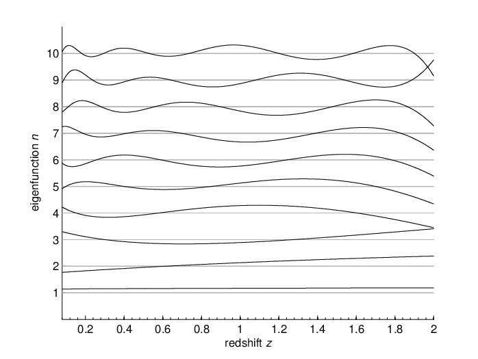
We first test the power of the data with the above technique. The primary basis functions are , . Other types of functions, such as and , are also tested but led to similar results. The function set leads to slightly larger reconstruction errors, while the reconstruction errors given by are slightly smaller than . In Fig.2, we show the first 10 normalized eigenfunctions obtained by fitting the data with PCA, with the underlying model being w = -1 and N = 10. We find that, for a fixed N, the shapes of eigenfunctions vary from smooth to oscillatory. The fiducial model used in this procedure has the same parameters as those used in the simulation procedures, i.e., and . We set and study three cases = 0.1, 0.5, and 1.0, respectively. Fig.3 shows the reconstructed (denote by hereafter). On the whole, the results are quite good for all values. Fig.3 shows that takes us from conservative models where = 1 to more wild models where = 0.1. This is due to the fact that models minimizing the BIC criteria tend to become smooth with tight error bars, while models with low AIC values are oscillatory and have large errors.

It is expected that the number of data points should have a crucial impact on the quality of the reconstruction. As shown in Fig.4, the reconstruction error drops drastically with an increasing number of the simulated data points, except for the number greater than 200 or so. For 200 or more data points, the resulting errors are comparable to what are shown in Fig.3. We can see that the currently observed 30 data points, with current measure quality, are really too sparse. We expect more OHD data points to be measured in future. On the other hand, 400 data points seem to be enough for improving the reconstruction quality, and further increasing the number of data points will merely lead to a marginal improvement. Further improvement on the reconstruction result needs further improvement on data quality.

However, it is unlikely that future surveys will provide hundreds of measurements. On the contrary, current measurements are basically systematic-dominated, so there is space for improvement in the direction of getting smaller errorbars, even at higher-z. Thus, we give the simulation by keeping the number 30 of data points fixed but reducing errors. How the reconstructed errors vary with different errors is shown in Fig.5. We can see that, to make the reconstructed error less than 0.05 at , which is equivalent to the reconstruction accuracy obtained by 400 points of current measurement quality (see Fig.4), the relative error of should achieve . Obviously this is a big challenge for future surveys. We alternatively test 50 points and find the needed relative error should be , and for 100 points the relative error is necessary. Considering the feasibility of future implement, 100 OHD measurements with quality of are desirable.

For comparison a hypothetical data set of distance modulus data is also constructed [10], which consists of 2000 data points evenly distributed in the redshift range , and 300 data points in range [31]. The uncertainties are composed of a constant statistical error and systematic errors linearly drifting from . The primary basis functions , , are transformed again to a set of eigenmodes with PCA, which are suitably adapted to the simulated data. The cosmological parameters are assumed, according to [10]. Different assumptions of in and simulations ( is set to 67.4 and 65 respectively) don’t affect the results. Fig.6 demonstrates the comparison between errors reconstructed from data and those reconstructed from simulated data. Red curves represent -reconstructed errors and blue curves represent -reconstructed errors. We find that for moderate values , both -reconstructed errors and -reconstructed errors are relatively low. When is greater than 0.6, however, the -reconstructed errors are lower than -reconstructed ones, and with the increase of , the differences between them get more remarkable. Increasing also vastly magnifies the differences. For smaller , in contrast to the -reconstructed errors, the -reconstructed errors will grow uncontrollably as increases. Only in the low- region does data produce errors greater than data. In addition, both -reconstructed and -reconstructed errors grow with decreased in the low- region ), and the differences between them are acceptable. Taken together, Fig.6 (see also Fig.4) shows that we can constrain the CDM model within at redshifts and even at 0.1 z 1 by using the simulated data. Thus, we conclude that using data can get better results than that using simulated data. Note that the mean relative errors of data are about , while the relative errors of data are about , indicating the former is nearly two orders larger than the latter (we compare the relative errors rather than the absolute values since and are different physical quantities). Hence, the comparison convincingly validates the merit of Hubble parameter data, as stated in section 2, in reconstructing the dark energy equation of state.

Based on the analysis in section 2, the reconstruction of from data can be split into two procedures: first reconstructing (denote by hereafter) from using Eq.(2), and then deriving from using Eq.(3). One may imagine that the error propagation and amplification taken in the first procedure will induce errors of similar in value to, or at least at the same order as, errors of data, so they would produce comparable errors (see Fig.6) for the resulting . However, Fig.7 shows this is not the case. We find from this figure that, compared to the errors of data, errors are quite small. We give the explanation as follows: first note that both and data are noisy, with errors measuring the extent of noise (see Fig.7). Because we use the first eigenfunctions, which encompass the dominant features in the data, to fit the data, and throw away the higher ones which contain noise-induced oscillations (see Methodology), noises are suppressed in the resultant . However, this is the case for reconstruction from data but not the case for reconstruction from data. By resampling the parameters in data fitting, noises are to a large extent suppressed in the first procedure of reconstruction from data (i.e., the procedure), resulting in relatively low errors (see Fig.7), while the second procedure (i.e., the procedure) essentially maintains all the noise-induced features inherited from the first procedure. In a word, it is the noise-suppression effect in the reconstruction of from data, which is lacking in the second procedure of reconstruction from data, that makes the reconstructed from behave better, even though the quality of data is much worse than data.

Then we use data to reconstruct two types of evolving . One is a standard slow evolution, expressed as ; the other evolves more drastically, modeled by . The reconstruction result is shown in Figs. 8 and 9. We set and . We again see that data outperform, in most cases, the simulated SN Ia data. Similar to the result obtained from the CDM model, the two evolving models are also constrained within for most redshifts in the range . For the second type of , not only the errors constructed by the former are much lower than the latter, but also the former constructed is more faithful to the underlying . It seems that data perform better for more oscillatory evolving dark energy.


4.2 Results on observational data
Finally we test the performance of OHD. See section 2 for the description of the OHD dataset of 30 data points. To make a comparison, the data set of distance modulus is also acquired. The last distance modulus measurements, which consist of 580 observed points, were produced by Supernova Cosmology Project11 1 http://supernova.lbl.gov/Union/ [16]. The parameters of the best-fit fiducial CDM model for OHD data are , while the parameters for fitting data are [10]. Interestingly, the most likely reconstruction, denoted , favors a transition from at low redshift to at higher redshift, a behavior that is consistent with the quintom model which allows to cross -1 [32]. The comparison of errors between -reconstructed and -reconstructed is given in Fig.11. We can see from Fig.11 that the quality of two reconstructions are comparable through most of the z region, though in low redshift region -reconstructed errors are noticeably larger than -reconstructed errors. Roughly speaking, the reconstruction from performs better than the reconstruction from for relatively large values. Concerning the much worse quality and much fewer observational data points of compared to , this result is impressive.

It is shown from Fig.10 that the shapes of the curves and are quite similar. Accordingly, as shown in Fig.11, the difference of error curves of for and are small, and the curve differs from the other two -reconstructed curves at a lower extent compared to the -reconstruction counterparts, especially in high redshift region. This behavior reveals that the reconstructions obtained from data are more “stable” than those from in the sense that they are less dependent on values. Here we can give an intuitive interpretation for it. The parameter in fact controls values and the number of combinations. The smaller is, the higher the probability that the larger, and the bigger the set of combinations is. Therefore, smaller results in the emergence of larger in the set of combinations, which leads to more precise data fitting and more noisy features reserved. Since is more "distant" from than , even small uncertainties included in the SN Ia data fitting curves may induce comparatively large oscillations of the resultant . On the contrary, for the reconstruction from OHD, the noisy features entering the eigenmodes due to the dropped s will not cause the resultant to oscillate significantly. Hence, from this aspect the merit of OHD in reconstructing dark energy equation of state is established more solidly.

5 Conclusions
We made an attempt in this paper to reconstruct dark energy equation of state parameter from Hubble parameter data within the framework proposed by Clarkson Zuncke [10]. We first made a comparison between the simulated Hubble parameter data and distance module data. The results showed that data can produce more conservative than the simulated data. Then the performance of OHD was evaluated against SNe data. We found that the errors of the reconstructed , using OHD and data, are comparable. We also concluded that the number of data points could impact the quality of the reconstruction. It turns out that 400 data points are sufficient to improve the reconstruction quality using OHD only. Further improvement requires more accurate data measurements.
We have shown that the Hubble parameter dataset alone is potentially capable of reconstructing the dark energy equation of state. As discussed above, to obtain satisfactory reconstruction, efforts on both the quality and the number of OHD are requisite. There are several ways to enhance the quality of OHD, of which deeper-redshift, more-complete-sky-coverage LRG survey and spectroscopic observations of those identified LRGs give remarkable improvement. It is expected that future surveys will be able to offer a large sample of massive and passive galaxies to be used in age-dating. The precise determination of the absolute galaxy ages is a quite complicated process, however, that issue can be ignored for measurements because one just needs to take the difference between the ages in narrow redshift bins so that the systematic bias in the absolute ages cancel out. The ongoing CMB observation program, the Atacama Cosmology Telescope (ACT) [33], will produce a catalogue of galaxy cluster candidates to be validated up to via the Sunyaev-Zel’dovich effect [34, 35]. This ensures a promising dataset outperforming current SNIa datasets. For the range , forthcoming surveys such as Euclid[36] and WFIRST [37], will greatly improve the present-day statistics, increasing the number of passive galaxies at these redshifts by at least an order of magnitude[36], which will result in observing approximatively one thousand spectra of passive galaxies at these redshifts[24]. Combining these future observations, it is reasonable to expect that the Hubble parameter data will be helpful in exploring the expansion history of the Universe.
It should be noted that the results and analyses in this paper are method-specific, since we consider just one reconstruction method. Whether similar results and conclusions can be obtained by using other reconstruction methods, such as Gaussian process modeling [5], is still unknown.
Acknowledgements
We would like to thank Dr. Hao-ran Yu and Hao-feng Qin for their in-depth discussion with us. This work was supported by the National Science Foundation of China (Grants Nos. 11173006, 11528306 and 11303003), the Ministry of Science and Technology National Basic Science program (project 973, grant No. 2012CB821804) and the Shandong Provincial Natural Science Foundation of China (Grant No ZR2013AM002).
References
References
- [1] M. Chevallier, D. Polarski, Accelerating Universes with Scaling Dark Matter, International Journal of Modern Physics D 10 (2001) 213–223. arXiv:gr-qc/0009008, doi:10.1142/S0218271801000822.
- [2] E. V. Linder, Exploring the Expansion History of the Universe, Physical Review Letters 90 (9) (2003) 091301. arXiv:astro-ph/0208512, doi:10.1103/PhysRevLett.90.091301.
- [3] A. Hojjati, L. Pogosian, G.-B. Zhao, Detecting features in the dark energy equation of state: a wavelet approach, JCAP 4 (2010) 7. arXiv:0912.4843, doi:10.1088/1475-7516/2010/04/007.
- [4] D. Huterer, A. Cooray, Uncorrelated estimates of dark energy evolution, Phys. Rev. D 71 (2) (2005) 023506. arXiv:astro-ph/0404062, doi:10.1103/PhysRevD.71.023506.
- [5] T. Holsclaw, U. Alam, B. Sansó, H. Lee, K. Heitmann, S. Habib, D. Higdon, Nonparametric Dark Energy Reconstruction from Supernova Data, Physical Review Letters 105 (24) (2010) 241302. arXiv:1011.3079, doi:10.1103/PhysRevLett.105.241302.
- [6] G.-B. Zhao, R. G. Crittenden, L. Pogosian, X. Zhang, Examining the Evidence for Dynamical Dark Energy, Physical Review Letters 109 (17) (2012) 171301. arXiv:1207.3804, doi:10.1103/PhysRevLett.109.171301.
- [7] R. A. Daly, S. G. Djorgovski, A Model-Independent Determination of the Expansion and Acceleration Rates of the Universe as a Function of Redshift and Constraints on Dark Energy, ApJ 597 (2003) 9–20. arXiv:astro-ph/0305197, doi:10.1086/378230.
- [8] A. Shafieloo, U. Alam, V. Sahni, A. A. Starobinsky, Smoothing supernova data to reconstruct the expansion history of the Universe and its age, MNRAS 366 (2006) 1081–1095. arXiv:astro-ph/0505329, doi:10.1111/j.1365-2966.2005.09911.x.
- [9] D. Majumdar, A. Bandyopadhyay, D. Adak, Reconstructing the equation of state and density parameter for dark energy from combined analysis of recent SNe Ia, OHD and BAO data, Journal of Physics Conference Series 375 (3) (2012) 032008. doi:10.1088/1742-6596/375/1/032008.
- [10] C. Clarkson, C. Zunckel, Direct Reconstruction of Dark Energy, Physical Review Letters 104 (21) (2010) 211301. arXiv:1002.5004, doi:10.1103/PhysRevLett.104.211301.
- [11] T. Holsclaw, U. Alam, B. Sansó, et al., Nonparametric reconstruction of the dark energy equation of state from diverse data sets, Phys. Rev. D 84 (8) (2011) 083501. arXiv:1104.2041, doi:10.1103/PhysRevD.84.083501.
- [12] H.-R. Yu, S. Yuan, T.-J. Zhang, Nonparametric reconstruction of dynamical dark energy via observational Hubble parameter data, Phys. Rev. D 88 (10) (2013) 103528. arXiv:1310.0870, doi:10.1103/PhysRevD.88.103528.
- [13] C. Ma, T.-J. Zhang, Power of Observational Hubble Parameter Data: A Figure of Merit Exploration, ApJ 730 (2011) 74. arXiv:1007.3787, doi:10.1088/0004-637X/730/2/74.
- [14] A. V. Pan, U. Alam, Reconstructing Dark Energy : A Comparison of Cosmological Parameters, ArXiv e-printsarXiv:1012.1591.
- [15] M. Moresco, L. Pozzetti, A. Cimatti, R. Jimenez, C. Maraston, L. Verde, D. Thomas, A. Citro, R. Tojeiro, D. Wilkinson, A 6% measurement of the Hubble parameter at z˜0.45: direct evidence of the epoch of cosmic re-acceleration, JCAP 5 (2016) 014. arXiv:1601.01701, doi:10.1088/1475-7516/2016/05/014.
- [16] N. Suzuki, D. Rubin, C. Lidman, et al., The Hubble Space Telescope Cluster Supernova Survey. V. Improving the Dark-energy Constraints above z > 1 and Building an Early-type-hosted Supernova Sample, ApJ 746 (2012) 85. arXiv:1105.3470, doi:10.1088/0004-637X/746/1/85.
- [17] D. Stern, R. Jimenez, L. Verde, M. Kamionkowski, S. A. Stanford, Cosmic chronometers: constraining the equation of state of dark energy. I: H(z) measurements, JCAP 2 (2010) 8. arXiv:0907.3149, doi:10.1088/1475-7516/2010/02/008.
- [18] M. Moresco, A. Cimatti, R. Jimenez, et al., Improved constraints on the expansion rate of the Universe up to z 1.1 from the spectroscopic evolution of cosmic chronometers, JCAP 8 (2012) 6. arXiv:1201.3609, doi:10.1088/1475-7516/2012/08/006.
- [19] N. G. Busca, T. Delubac, J. Rich, et al., Baryon acoustic oscillations in the Ly forest of BOSS quasars, AA 552 (2013) A96. arXiv:1211.2616, doi:10.1051/0004-6361/201220724.
- [20] C. Zhang, H. Zhang, S. Yuan, S.and Liu, T.-J. Zhang, Y.-C. Sun, Four new observational H(z) data from luminous red galaxies in the Sloan Digital Sky Survey data release seven, Research in Astronomy and Astrophysics 14 (2014) 1221–1233. arXiv:1207.4541, doi:10.1088/1674-4527/14/10/002.
- [21] C. Blake, S. Brough, M. Colless, et al., The WiggleZ Dark Energy Survey: joint measurements of the expansion and growth history at z 1, MNRAS 425 (2012) 405–414. arXiv:1204.3674, doi:10.1111/j.1365-2966.2012.21473.x.
- [22] C.-H. Chuang, Y. Wang, Modelling the anisotropic two-point galaxy correlation function on small scales and single-probe measurements of H(z), DA(z) and f(z)8(z) from the Sloan Digital Sky Survey DR7 luminous red galaxies, MNRAS 435 (2013) 255–262. arXiv:1209.0210, doi:10.1093/mnras/stt1290.
- [23] T. Delubac, Bautista, J. E., N. G. Busca, et al., Baryon acoustic oscillations in the Ly forest of BOSS DR11 quasars, AA 574 (2015) A59. arXiv:1404.1801, doi:10.1051/0004-6361/201423969.
- [24] M. Moresco, Raising the bar: new constraints on the Hubble parameter with cosmic chronometers at z 2, Mon. Not. R. Astron. Soc. 450 (2015) L16–L20. arXiv:1503.01116, doi:10.1093/mnrasl/slv037.
- [25] Planck Collaboration, P. A. R. Ade, N. Aghanim, et al., Planck 2013 results. XVI. Cosmological parameters, AA 571 (2014) A16. arXiv:1303.5076, doi:10.1051/0004-6361/201321591.
- [26] O. Farooq, B. Ratra, Hubble Parameter Measurement Constraints on the Cosmological Deceleration-Acceleration Transition Redshift, ApJL 766 (2013) L7. arXiv:1301.5243, doi:10.1088/2041-8205/766/1/L7.
- [27] E. Gaztañaga, A. Cabré, L. Hui, Clustering of luminous red galaxies - IV. Baryon acoustic peak in the line-of-sight direction and a direct measurement of H(z), MNRAS 399 (2009) 1663–1680. arXiv:0807.3551, doi:10.1111/j.1365-2966.2009.15405.x.
- [28] A. Heavens, R. Jimenez, L. Verde, Standard Rulers, Candles, and Clocks from the Low-Redshift Universe, Physical Review Letters 113 (24) (2014) 241302. arXiv:1409.6217, doi:10.1103/PhysRevLett.113.241302.
- [29] I. Maor, R. Brustein, J. McMahon, P. J. Steinhardt, Measuring the equation of state of the universe: Pitfalls and prospects, Phys. Rev. D 65 (12) (2002) 123003. arXiv:astro-ph/0112526, doi:10.1103/PhysRevD.65.123003.
- [30] V. Sahni, A. Shafieloo, A. A. Starobinsky, Two new diagnostics of dark energy, Phys. Rev. D 78 (10) (2008) 103502. arXiv:0807.3548, doi:10.1103/PhysRevD.78.103502.
- [31] SNAP Collaboration: G. Aldering, W. Althouse, R. Amanullah, et al., Supernova / Acceleration Probe: A Satellite Experiment to Study the Nature of the Dark Energy, ArXiv Astrophysics e-printsarXiv:astro-ph/0405232.
- [32] B. Feng, X. Wang, X. Zhang, Dark energy constraints from the cosmic age and supernova, Physics Letters B 607 (2005) 35–41. arXiv:astro-ph/0404224, doi:10.1016/j.physletb.2004.12.071.
- [33] http://www.physics.princeton.edu/act/index.html.
- [34] J. Simon, L. Verde, R. Jimenez, Constraints on the redshift dependence of the dark energy potential, Phys. Rev. D 71 (12) (2005) 123001. arXiv:astro-ph/0412269, doi:10.1103/PhysRevD.71.123001.
- [35] R. R. Lindner, P. Aguirre, A. J. Baker, J. R. Bond, D. Crichton, M. J. Devlin, T. Essinger-Hileman, P. Gallardo, M. B. Gralla, M. Hilton, A. D. Hincks, K. M. Huffenberger, J. P. Hughes, L. Infante, M. Lima, T. A. Marriage, F. Menanteau, M. D. Niemack, L. A. Page, B. L. Schmitt, N. Sehgal, J. L. Sievers, C. Sifón, S. T. Staggs, D. Swetz, A. Weiß, E. J. Wollack, The Atacama Cosmology Telescope: The LABOCA/ACT Survey of Clusters at All Redshifts, APJ 803 (2015) 79. arXiv:1411.7998, doi:10.1088/0004-637X/803/2/79.
- [36] R. Laureijs, J. Amiaux, S. Arduini, J. . Auguères, J. Brinchmann, R. Cole, M. Cropper, C. Dabin, L. Duvet, A. Ealet, et al., Euclid Definition Study Report, ArXiv e-printsarXiv:1110.3193.
- [37] D. Spergel, N. Gehrels, J. Breckinridge, M. Donahue, A. Dressler, B. S. Gaudi, T. Greene, O. Guyon, C. Hirata, J. Kalirai, N. J. Kasdin, W. Moos, S. Perlmutter, M. Postman, B. Rauscher, J. Rhodes, Y. Wang, D. Weinberg, J. Centrella, W. Traub, C. Baltay, J. Colbert, D. Bennett, A. Kiessling, B. Macintosh, J. Merten, M. Mortonson, M. Penny, E. Rozo, D. Savransky, K. Stapelfeldt, Y. Zu, C. Baker, E. Cheng, D. Content, J. Dooley, M. Foote, R. Goullioud, K. Grady, C. Jackson, J. Kruk, M. Levine, M. Melton, C. Peddie, J. Ruffa, S. Shaklan, Wide-Field InfraRed Survey Telescope-Astrophysics Focused Telescope Assets WFIRST-AFTA Final Report, ArXiv e-printsarXiv:1305.5422.