Holographic phase transitions from higgsed, non abelian charged black holes
Abstract
We find solutions of a gravity-Yang-Mills-Higgs theory in four dimensions that represent asymptotic anti-de Sitter charged black holes with partial/full gauge symmetry breaking. We then apply the AdS/CFT correspondence to study the strong coupling regime of a quantum field theory at temperature and finite chemical potential, which undergoes transitions to phases exhibiting the condensation of a composite charged vector operator below a critical temperature , presumably describing -wave superconductors. In the case of -wave superconductors the transitions are always of second order. But for -wave superconductors we determine the existence of a critical value of the gravitational coupling (for fixed Higgs v.e.v. parameter ) beyond which the transitions become of first order. As a by-product, we show that the -wave phase is energetically favored over the one, for any values of the parameters. We also find the ground state solutions corresponding to zero temperature. Such states are described by domain wall geometries that interpolate between spaces with different light velocities, and for a given , they exist below a critical value of the coupling. The behavior of the order parameter as function of the gravitational coupling near the critical coupling suggests the presence of second order quantum phase transitions. We finally study the dependence of the solution on the Higgs coupling, and find the existence of a critical value beyond which no condensed solution is present.
1 Introduction
In recent years the application of AdS/CFT or more generally gauge/gravity correspondence [1] [2] [3] to the study of condensed matter physics has attracted a lot of attention, providing in particular gravitational descriptions of systems exhibiting superconductor/superfluid phases [4] [5]. Since in condensed matter physics we are typically dealing with systems at finite charge density and temperature, in the context of the AdS/CFT correspondence the dual gravity descriptions should be given in terms of gravitational models with a negative cosmological constant which admit charged black holes as vacuum solutions. In fact, a charged black hole naturally introduces a charge density/chemical potential and temperature in the quantum field theory (QFT) defined on the boundary using the gauge/gravity correspondence. This set-up allows in particular to study phase transitions and construct phase diagrams in parameter space.
The simplest model is provided by an Einstein-Maxwell theory coupled to a charged scalar field that, in the framework of the AdS/CFT correspondence, is dual to a scalar operator which carries the charge of a global symmetry. It has been shown that a charged black hole solution, interpreted as the uncondensed phase, becomes unstable and develops scalar hair at low temperature breaking the symmetry near the black hole horizon [6] [7]. This phenomenon in general may be interpreted as a second order phase transition between conductor and superconductor phases, interpretation that is supported by analyzing the behavior of the conductivity in these phases [5]. There were also studied vortex like solutions that describe type II holographic superconductors [8] [9] [10] and more recently, spatially anisotropic, abelian models of superconductors [11].
Soon after these “-wave” holographic superconductor models were introduced, holographic superconductors models with vector hair, known as -wave holographic superconductors, were explored numerically first in [12] and [13] (for a recent analytical treatment, see [14]). The simplest example of -wave holographic superconductors may be provided by an Einstein-Yang-Mills theory with gauge group and no scalar fields, where the electromagnetic gauge symmetry is identified with an subgroup of . The other components of the gauge field play the role of charged fields dual to some vector operators whose non-zero expectation values break the symmetry leading to a phase transition in the dual field theory.
More recently, solutions to gravity-matter field equations where both scalar and vector order parameters are present were considered; they describe systems where competition/coexistence of different phases takes place [15]-[18].
Regular, self-gravitating dyonic solutions of the Einstein-Yang-Mills-Higgs (EYMH) equations in the BPS limit and asymptotic to global AdS space, were constructed time ago in [19] and [20]. They were extended to dyonic black hole solutions in [21] and [22], where they were interpreted as describing a so-called -wave superconductor (isotropic) system at finite temperature in the condensed phase. The purpose of the present work is to generalize previous results by finding more general black hole solutions of EYMH in asymptotically space with finite mass and electric charge density, to interpret them via the gauge/gravity duality as describing phases of a strongly coupled field theory, and to construct the corresponding phase diagrams 11 1 We will be considering the usual plane horizon ansatz, relevant to study condensed matter systems with translational invariance. Under these circumstances, the magnetic charge density of the dyon solutions in [21] [22] disappears. . More specifically, in first term we start by revisiting the analysis of [21] [22], verifying the existence of second order phase transitions all along the parameter space. It was found (see for example [23]) that some holographic systems pass from a second order phase transition as a function of the temperature in the non back-reaction limit to a first order when the gravitational coupling exceeds a certain value. Such a phenomenon occurs in holographic superfluids when the velocity is high enough [24] [25], and it was measured in certain types of superconductors [26] [27] [28]. We have found this kind of behavior in our system in the anisotropic case, finding condensed solutions and constructing the phase diagram. Second, we compute free energies and find that for any set of values of the free parameters that determines the solutions, the anisotropic phase is energetically favored over the isotropic phase, as conjectured in other contexts [29] [30] [31]. Third, we analyze the zero temperature limit, case that had not been addressed before; for low enough gravitational coupling we find solutions which spontaneously break the symmetry and have zero entropy, and so describe the true ground state of the system. For gravitational couplings higher than a critical value the solution disappears, which is interpreted as a second order quantum phase transition. Lastly, we study the effect of a non zero Higgs potential on the system.
The paper is organized as follows. In section we present the model and write the translational invariant ansatz for the fields and the equations of motion that reduces to a a nonlinear system of coupled ordinary differential equations. In section we present generalities of the systems to be studied at non-zero temperature, in particular the analysis of the holographic map to be used. In section we present the numerical results concerning the “BPS limit”, i.e. null Higgs potential, including computations of free energies. Section is devoted to the study of the zero temperature case and the description of the ground state of the superconductor, including the presence of quantum phase transitions as function of the gravitational coupling and variable Higgs vacuum expectation value (vev) . In section the effect of a non-zero Higgs potential is considered. A summary and discussion of the results is given in section . Finally two appendices are added, one containing the boundary expansions of the fields and other containing the equations of motion and free energy in other parameterization commonly used in the literature.
2 The gravity-Yang-Mills-Higgs system
2.1 The model
We consider a gravity-Yang-Mills-Higgs system in a dimensional space-time with Minkowski signature . We take as the gauge group, with generators satisfying the algebra,
| (2.1) |
and the scalar field in the adjoint representation, . The full action to be considered is,
| (2.2) |
where
| (2.3) | |||||
| (2.4) | |||||
| (2.5) |
where , and are the gravitational, gauge and scalar couplings respectively, is the AdS scale related to the negative cosmological constant through , and defines the vacuum expectation value of the Higgs field (and so the boundary condition at infinity, see below in (2.32)). As it is well-known, the Gibbons-Hawking term is necessary to have a well defined variational principle [32], where is the trace of the extrinsic curvature, and and the induced metric and normal vector on . The counter-term action will be discussed in section 4.
The field strength and the covariant derivative acting on the Higgs triplet are defined as,
| (2.6) |
Let us consider coordinates and an ansatz preserving translational invariance in the coordinates ,
| (2.7) | |||||
| (2.8) | |||||
| (2.9) |
In what follows it will be convenient to introduce the dimensionless coupling constants,
| (2.10) |
The gravity equations of motion (e.o.m.) derived from (2.3) result,
| (2.11) | |||||
| (2.12) | |||||
| (2.13) | |||||
| (2.14) | |||||
| (2.15) | |||||
| (2.16) |
while that the matter e.o.m. are,
| (2.17) | |||||
| (2.18) | |||||
| (2.19) | |||||
| (2.20) |
where we have defined,
| (2.21) |
We will start by considering the “BPS limit” , but conserving the crucial Higgs vacuum value . The effect of a finite Higgs coupling will be considered in section .
2.2 Boundary conditions
We will search for charged black hole solutions which present a horizon at where . The associated Bekenstein-Hawking temperature of the black hole is given by,
| (2.22) |
The ansatz (and e.o.m.) are invariant under the scale transformations,
| (2.23) | |||||
| (2.24) |
They allow to fix some normalization imposing the b.c., , in such a way that the ’s are identified with the minkowskian coordinates of the boundary QFT, and (2.22) with its temperature. Furthermore there exists another scaling symmetry,
| (2.25) |
that if , allows to fix 22 2 This is the case except when we consider the zero temperature limit. When back-reaction is not taking into account corresponds to AdS space; when it is considered, is imposed in order to get a true ground state description and (2.25) can be used to fix the chemical potential, see section 5. . Since now on we will fix the position of the horizon in this way, having in mind that we have to consider only scale invariants quantities.
In [21] and [22] solutions to (2.11)-(2.17) with a horizon and asymptotically were studied. More specifically, there were found solutions with and the following boundary conditions; near the horizon ,
| (2.26) | |||||
| (2.27) | |||||
| (2.28) | |||||
| (2.29) | |||||
| (2.30) | |||||
| (2.31) |
while on the boundary ,
| (2.32) | |||||
| (2.33) | |||||
| (2.34) | |||||
| (2.35) | |||||
| (2.36) | |||||
| (2.37) |
where consistency with the e.o.m. and finiteness of fixes to be,
| (2.38) |
For more about the b.c. at the boundary, we refer the reader to the appendix A. We will adopt the b.c. (2.26)-(2.32) in this paper except in section 5 where the b.c. on the horizon will have to be modified.
The bulk theory is invariant under the gauge group ; however the b.c. on the Higgs field, , breaks this invariance to the generated by . With respect to this gauge subgroup the electric charge density of a solution is defined as usual by,
| (2.39) |
As we show in section 4, at fixed couplings a general solution to (2.11)-(2.17) with the b.c. (2.26)-(2.32) is determined by , which is related to the chemical potential by,
| (2.40) |
From (2.39) and (2.40) the standard asymptotic expansion follows,
| (2.41) |
Along this paper we will adopt as our scale. From (2.25) the dimensionless, scale invariant temperature is,
| (2.42) |
where and are defined in (2.26). A solution is determined by the three free parameters (), and so the temperature (through the coefficients , ) results a function of them 33 3 In EYM systems where the Higgs field is not present the temperature is function of the only free parameter of the theory, , see [23]. .
In the analytic solution to the equations (2.11)-(2.17) that preserves the symmetry matter fields take the form,
| (2.43) |
where we imposed smooth behavior of the gauge field at the horizon which yields the condition , see the last line in (2.26), and then fixed 44 4 When , is just the chemical potential and the metric solution is AdS space; it describes the uncondensed phase when the temperature is zero, see section . . In what the metric functions concern, they correspond to the AdS Reissner-Nordström (AdS-RN) black hole,
| (2.44) | |||||
| (2.45) | |||||
| (2.46) |
with temperature,
| (2.47) |
The extremal, zero temperature AdS-RN black hole is defined by the relation .
3 Solutions at : superconducting state
When the “magnetic part” of the gauge field is non-trivial, i.e. for some , the solution breaks not only the invariance, but also the invariance under rotations in the -plane. According to the AdS/CFT dictionary this hair is interpreted as a spontaneous breaking of a global symmetry present in the boundary QFT, whose currents take an expectation value,
| (3.1) |
Giving that the order parameter is dual to (a component of) the gauge field we are presumably modeling a -wave superconductor [13]. The normal state of the superconductor is described by the AdS-RN solution (2.43)-(2.44); such solution is energetically favored until a critical temperature is reached; when the non symmetric, hairy solution gives rise to a superconductor phase.
We remark that with the b.c. on the Higgs field we are breaking explicitly the gauge group from to ; this yields a mass for the “W” gauge bosons,
| (3.2) |
The problem is thus the following: can we find under this condition a solution with that breaks spontaneously the ? In the boundary QFT this is then interpreted as the breaking of a global symmetry as it happens in superfluids and superconductors with weakly coupled photons. From here we identify with the critical temperature of the phase transition in the QFT.
We will consider two cases.
- •
The isotropic case:
Although both gauge and rotational symmetries are broken by a hairy solution, a configuration with preserves the diagonal subgroup, , fact that is manifest in (3.1) [12]. This configuration give rise to an energy-momentum tensor isotropic in the - plane; therefore the metric function must be a constant, even when back-reaction is taken into account.
- •
The anisotropic case:
As stated above, a configuration with preserves the and spatial rotations. When develops a non zero value the gauge symmetry breaks, and the condensate choose a direction as a special one. Then if we take into account back-reaction effects the system cannot support the condition [13]. Due to this fact and the function can not be a constant; in conclusion the system will be in an anisotropic phase.
In both cases the vacuum expectation value in the field theory of the current operator , dual to the function associated with the magnetic field in the bulk, follows from the identification, with defined in (2.32); can be taken as the order parameter that describes the phase transition of the system. As discussed for different models [7]-[22] one can interpret this result by stating that a condensate is formed above a black hole horizon because of a balance of gravitational and electrostatic forces. From the asymptotic behavior in (2.32) we get the dimension of the operator [33]
| (3.3) |
From numerical solutions we conclude that a finite temperature continuous symmetry breaking transition takes place so that the system condenses at a critical temperature , as can be seen from the behavior of for in figures , and . Furthermore, we compare the free energies corresponding to both phases in figures and , finding that the anisotropic phase is favored, see [29] [30] [31] for related results.
4 Numerical Solutions
We analyzed numerically equations (2.11)-(2.17) and found solutions that satisfy the required b.c. (2.26)-(2.32) in a wide region of the parameter space, that lead to the phase diagram in figure . Such solutions in the anisotropic case are shown in figure .
Before presenting the results, we think is worth to spend a few words on the method used. As discussed in appendix A, after fixing some normalization and asking for finiteness the solution near the boundary admits the expansions in equation (A.1), and is determined by six constants, . However the b.c. on the horizon impose five conditions. The first two come from the definition of the horizon and the regularity of the gauge field,
| (4.1) |
They essentially fix the mass () and the charge density () of the black hole. The remaining three conditions fix and are obtained from an analysis of the (singular) behavior of the e.o.m. near the horizon,
| (4.2) | |||||
| (4.3) | |||||
| (4.4) |
Therefore the only additional free parameter that determines the solution is , i.e. the chemical potential (2.40). In practice we integrate the system from the horizon, where according to (4.1)-(4.2) the free parameters are,
| (4.5) |
as defined in (2.26). These parameters are selected in such a way that the solution matches the conditions on the boundary ,
| (4.6) |
.


Figure displays the phase diagrams in the plane, for two different values of . In the white regions only the normal or uncondensed phase is present. In the isotropic case the system experiments second order phase transitions along the blue () and green () curves. In the anisotropic case, in the blue and red regions the condensed phase is the thermodynamically preferred phase. The blue line until the black point indicates a critical line of second order transitions. The black point signals the coupling beyond which the transitions become of first order along the red line, while that the blue and green lines that continue after this tri-critical point represent spinodal lines. The critical red curve of first order phase transitions ends in the red point at , which represents a quantum phase transition, signaling a critical coupling above which the condensed phase ceases to exist, see Section 5. By comparing both graphs we can see that both and decrease with increasing . Similar phase diagrams were obtained in reference [34] in absence of Higgs fields.
In figure the fields are shown as functions of the coordinate , at fixed and and for different ’s. For a second horizon appears, as displayed from the curves corresponding to . The uncondensed and condensed phases are separated by a curve on which the formation of the second horizon takes place for a given critical temperature determined by the gauge boson mass and . In the isotropic case the curve is displayed in figure for two different values of (blues and green lines) and it coincides with the critical curve on which the phase transitions take place. On the other hand, in the anisotropic case the curve coincides with the critical curve (blue line in figure ) until the tri-critical point , and it continues through the spinodal curve in green.
In figure the order parameter in the isotropic case is plotted as a function of the temperature for different values of , at fixed gravitational coupling . In this case the transition is of second order independently of , in agreement with [12].
Figures and shows the order parameter as function of in the anisotropic case from two perspectives: at fixed and varying in figure and at fixed and varying in figure . From figure it is seen that for becomes multi-valued, fact that signals the passage from second to first order phase transitions as corroborated from the free energy computations of the next subsection. This phenomenon has been found recently in -wave superfluids by studying the role of the back-reaction in the phase transitions [23] (for experimental results on first order phase transitions in superconductors, see [26][27][28]). By comparing figures and it is observed that the temperature at which the order parameter becomes zero is the same in both cases, and that the critical temperature decreases when increases, what can be interpreted as the presence of the Higgs field hinders the condensation. Furthermore, we have checked that near and for weak gravitational couplings , behaves like , indicating a second order phase transition with mean field exponent as usually happens in holographic descriptions of critical systems in the limit of large number degrees of freedom.


4.1 The free energy
According to the AdS/CFT correspondence, the free energy of the QFT is given by,
| (4.7) |
From (2.3) and using the e.o.m. the bulk contribution to the free energy density can be written as,
| (4.8) | |||||
| (4.9) | |||||
| (4.10) |
The Gibbons-Hawking contribution is,
| (4.11) |
Here we have introduced to regularize the expressions since they present divergent terms. To this end we introduce a counter-term action [35] [36],
| (4.12) |
which give rise to the following contribution to the free energy density,
| (4.13) |
The total free energy density of the system is then given by,
| (4.14) |
We remark that in order to analyze the results the right thing to do is to work with the scale invariant free energy density,
| (4.15) |
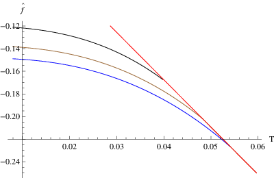
Figures and show the evolution of the free energy density (4.15) with the mass of the gauge boson for two different values of , in the isotropic and anisotropic cases respectively. Figure displays the continuity of at the critical temperature (where the free energy density of the uncondensed phase intersects the curve of the condensed phase) for both values of , for any , fact that indicates the second order character of the phase transition as the behavior of in figure suggested. In figure instead it is observed the discontinuity in the first derivative of the free energy density at the critical temperature for for any , signaling a first order phase transition. In both cases the critical temperature decreases with growing , in agreement with the analysis of the behavior of the order parameter made above.
In figures and the free energy densities of the isotropic and anisotropic phases are compared for two values of the gravitational coupling, (figure ) and (figure ). From them one can see that the free energy density of the anisotropic phase, no matter the region where the value of is, i.e. if first or second order phase transitions take place, is lower than the free energy density of the isotropic phase. That is, the anisotropic phase is always energetically favored over the isotropic one.


5 Zero temperature solutions
In this section we will address the problem of quantum phase transitions in three dimensional -wave superconductors (anisotropic case), i.e. transitions at , that to our knowledge was not considered before in the literature (see however [37] [38] [39] [40] for related studies in other settings).
It is known that when a charged AdS black hole is driven to a state of zero temperature it becomes extremal, but its entropy is different from zero and then it can not describe the ground state of the superconductor that we are presumably modeling holographically. To reach our goal the radius of the black hole needs to become null, to agree with the third law of thermodynamics and really describe the quantum ground state [29] [41]. So we must impose that , i.e. the coordinate . A very important thing from a technical point of view is that while the asymptotic behavior of the fields is as in (2.32), the expansions near the horizon drastically change with respect to the case. At leading order the (non analytical) behavior of the fields for is,
| (5.1) | |||||
| (5.2) | |||||
| (5.3) | |||||
| (5.4) | |||||
| (5.5) | |||||
| (5.6) |
The independent constants are . Such constants are chosen in the same way as in the case, see (4.6). From (5.1) it follows that near the horizon the solution is another space. The solutions that describe the quantum ground state of the superconductor in the condensed phase are therefore domain walls interpolating spaces with the same radius but different light velocities in both directions, in virtue of the fact that and . More explicitly,
| (5.7) |
On the other hand, the uncondensed phase is described strictly by space and , which replace the AdS-RN solution (2.43)-(2.44). Interestingly, we found that above a certain the solution representing the condensed phase disappears and the only solution that exists is AdS space. This result can be guessed from the following analysis borrowed from [38] (see also [29]). At very low temperatures the normal phase is nearly represented by the extremal, zero temperature Reissner-Nördstrom solution (2.43-2.47) with , whose near horizon geometry is . If we perturb this solution with a non-zero gauge field , from the first equation in (2.17) its linear equation in this background results,
| (5.8) |
where , which is just the wave equation for with an effective mass,
| (5.9) |
So, the instability to form vector hair at low temperature is just that of scalar fields below the BF bound for , . That is, when one could wait that AdS vacuum gets unstable and the system prefers to be in the phase described by the superconducting black hole solution with non abelian hair. Thus we get a plausible condition for instability,
| (5.10) |
Figure shows the fields for different values of the gravitational coupling 55 5 We use the scaling symmetry (2.25) to fix . . In the example showed () we obtain , see figures and .


We worked out the solutions for different values of the parameter , in Table I the corresponding critical couplings are shown. It is observed that decreases with growing and that , what is consistent with the instability analysis made before.
On the other hand, in Figure it is shown the order parameter as a function of the coupling . We have verified that the behavior near the critical coupling is of the type,
| (5.11) |
consistent with the existence of a second order phase transition in the mean field, large number of degrees of freedom limit.

| 1.03 | |
| 0.97 | |
| 0.94 | |
| 0.88 | |
| 0.86 | |
| 0.84 | |
| 0.80 | |
| 0.76 | |
| 0.74 | |
| 0.70 |
6 Analysis for
In this section we will study the effect of a non-zero Higgs potential as introduced in (2.3), specified by the Higgs vev scale and the strength . For simplicity we will work in the no back-reaction limit , although the new insights does not depend on this fact.
In the conventions of Appendix B, the e.o.m. (2.17) in the anisotropic case reduce to,
| (6.1) | |||||
| (6.2) | |||||
| (6.3) |
where .
The existence of a non-zero does not modify the behavior of and on the boundary that remain as in (2.32), but it does in the Higgs case where we now have,
| (6.4) |
where, for general and ,
| (6.5) |
A first well-known fact is that reality of necessarily implies the BF bound . When we are in the window both modes are normalizable and lead to consistent quantization and we can impose or . If , the condition must be imposed [42]. We will consider for definiteness the case .
A very interesting fact is that, besides the existence of a bound from below for the Higgs coupling as stated above, a straight analysis of the solution near the boundary yields the result that a bound from above is also present. We find that there exists a critical value defined by,
| (6.6) |
such that for the condensed solution ceases to exist. In the example considered below , . This is so for both the isotropic and anisotropic cases.
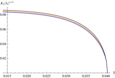
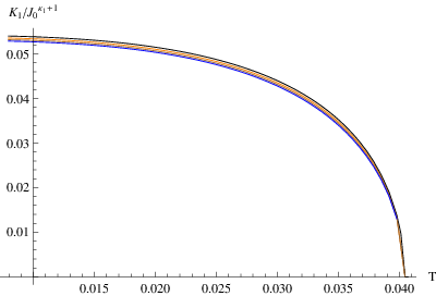

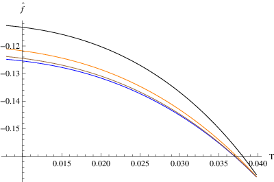


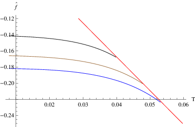
Figures and show the condensate and the free energy respectively as functions of the temperature, for a fixed and different Higgs couplings 66 6 For higher Higgs strengths towards the critical value the curves does not experiment significative changes. . One can appreciate that both the order parameter and the free energy decreases with increasing strength of the potential ; however the critical temperature does not change and the phase transitions remain of second order.
In Figure the free energies of both isotropic and anisotropic cases as functions of the temperature are plotted together for comparison, for fixed Higgs scale and different Higgs couplings. The anisotropic phase always remains energetically favored over the isotropic one.
As stated before, a critical value (6.6) above which the condensed phase does not exist is present, and it was verified by our numerical calculations; such result occurs in both isotropic and anisotropic cases.
Figures show the free energies in function of the temperature for a fixed , for different gauge boson masses. It is observed that they increase with increasing . The curves are similar to the left curves in figures and .
7 Conclusions and outlook
In this paper we have investigated four dimensional solutions of black holes with non-abelian, hair introduced by Yang-Mills gauge bosons and a non trivial Higgs field in the adjoint representation, whose v.e.v. triggers the breaking of the gauge symmetry to a subgroup under which the black hole is charged.
In the spirit of the AdS/CFT correspondence, the symmetric solution given by the AdS-RN black hole when the temperature is positive and AdS when , describes the uncondensed phase of the dual three dimensional QFT. A solution with non-abelian hair generically breaks the gauge symmetry together with the rotational symmetry, and is interpreted as describing a condensed phase of the QFT. The order parameter is the coefficient of the leading order term of the magnetic component of the gauge field, and thus the systems described are generically termed -wave superfluids/superconductors. We have considered two cases. The isotropic case that describes -wave superconductors where the diagonal subgroup of is preserved, and the anisotropic case where no symmetry is preserved. In both cases we get phase transitions at critical temperatures that decrease when the gravitational coupling grows and in the case of anisotropic superconductors the phase transitions become of first order for large gravitational couplings [23]. These results are summarized in the phase diagrams presented in figure .
We also find solutions that describe the zero entropy ground state of the -wave superconductor, showing the existence of phase transitions from the normal phase (described by AdS space) to this condensed phase, that is present below a certain value of the gravitational coupling . These transitions are of second order, according to the behavior (5.11) of the order parameter near the transition obtained from figure . Such states are described by domain wall geometries that interpolate two AdS spaces. The occurrence of AdS space near the horizon, with the the same scale as the AdS in the boundary but different light velocities, presumably indicates that there is an emergent scale invariance in the limit [23] [24].
Finally we study the effect of considering a non zero Higgs potential. It was found that for Higgs coupling constants greater than a critical value , the solution collapses to the normal one. This fact relies on the ultraviolet behavior of the system; in particular is independent if the back-reaction is considered or not. For below the system and its thermodynamic variables behave qualitatively as in the case , but with lower free energy.
A very relevant fact conjectured in the literature [12] [13] [29] for systems without Higgs fields that we have explicitly addressed in this paper including them together with the corresponding Higgs potential, is that below the critical temperature in all the parameter space we found that the free energy density of the anisotropic solution is lower than that of the isotropic one, indicating that the -wave superconductor phase is more stable that the one corresponding to the -wave superconductor. This result is illustrated in figures , and .
We believe it is worth to make the following remarks. It is straight to see that if we switch off the Higgs field the e.o.m. of the -wave superconductor are recovered. However if we switch off the magnetic part of the gauge field, , it is seen that we do not recover the e.o.m. of a -wave superconductor. This is due to the fact that we are switching the Higgs field in the -direction, not in the -direction. This lead us to conclude that in our set-up the Higgs field can not condense spontaneously since the temporal component of the gauge field (which plays a fundamental role in the condensation) is null. Therefore we will never have competition between s-wave and p-wave phases, as it takes place in the cases analyzed in references [15]-[18] where the matter field ansatz is slightly different and the vev Higgs field is put to zero. Furthermore it is not difficult to see from the e.o.m. that a configuration where a vev (3.1) is present necessary implies a non-trivial Higgs field; however the vev of its dual scalar operator ,
| (7.1) |
does not indicate any spontaneous breaking in view of the presence of the source .
We stress that, although they share some similar characteristics, the presence of the Higgs fields with the non trivial b.c. , introduces a scale that makes our systems different from those considered in precedence since [13] [37], in which the scalars were not present. On one hand from the obvious fact that the system is larger and more complex; in particular we have three free parameters () and, among other things, the dimension (3.3) of the order parameter remains arbitrary. Instead, in EYM systems where the Higgs field is not present, the temperature for example is a function of just one parameter [23]. On the other hand and more important, from the QFT point of view to which the systems we have considered are presumed to be holographically dual. This fact can be elucidate by studying the transport properties of the system, i.e. the conductivities. Even ignoring back-reaction effects, we finish with a system of fifteen coupled second order equations that results much more cumbersome to disentangle than in the Abelian case or in the absence of Higgs fields. We hope to report results in this direction in a near future [43].
Acknowledgments
We would like to thank Nicolás Grandi and Ignacio Salazar Landea for encouragement and continuous support, and Borut Bajc, Jorge Russo and Gastón Giribet for careful reading of the manuscript and useful comments. This work was supported in part by CONICET, Argentina.
Appendix A Boundary expansions
Along this paper we used shooting methods to get the solutions to the e.o.m. We present here the (next to) leading order behavior of the fields near the boundary that is necessary to carry out the numerics.
For large the fields admit the expansions,
| (A.1) | |||||
| (A.2) | |||||
| (A.3) | |||||
| (A.4) | |||||
| (A.5) | |||||
| (A.6) |
where , etc., for . The constants are free, all the other ones as well the powers (including those make explicit in (A.1)) are determined by the e.o.m. 77 7 The boundary conditions at the horizon leave just one free parameter (that we take ) that determines completely the solution, see Section 4. In the isotropic case, , , they are given by,
while that in the anisotropic case, , they result,
| (A.19) | |||||
| (A.24) | |||||
Appendix B AH conventions
In this appendix we write the e.o.m. in the conventions of references [23], [44]. Besides being often present in literature, they proved to be convenient in some numerical computations.
The ansatz is written as,
| (B.1) | |||||
| (B.2) | |||||
| (B.3) |
The relation with the conventions used in the bulk of the paper are,
| (B.4) | |||
| (B.5) | |||
| (B.6) |
The gravity e.o.m. result (out the tildes),
| (B.7) | |||||
| (B.8) | |||||
| (B.9) |
where are the r.h.s.’s of (2.11) written in the variables (B.4), while that the matter e.o.m. are,
| (B.10) | |||||
| (B.11) | |||||
| (B.12) | |||||
| (B.13) |
Finally, the contributions to the free energy density are,
| (B.15) | |||||
| (B.16) | |||||
| (B.17) | |||||
| (B.18) | |||||
| (B.19) |
References
- [1] J. M. Maldacena, “The large N limit of superconformal field theories and supergravity,” Adv. Theor. Math. Phys. 2 (1998) 231 [Int. J. Theor. Phys. 38 (1999) 1113] [arXiv:hep-th/9711200].
- [2] S. S. Gubser, I. R. Klebanov and A. M. Polyakov, “Gauge theory correlators from non-critical string theory,” Phys. Lett. B 428 (1998) 105 [arXiv:hep-th/9802109].
- [3] E. Witten, Adv. Theor. Math. Phys. 2 (1998) 253 [arXiv:hep-th/9802150].
- [4] S. A. Hartnoll, C. P. Herzog and G. T. Horowitz, “Building a Holographic Superconductor,” Phys. Rev. Lett. 101 (2008) 031601 [arXiv:0803.3295 [hep-th]].
- [5] S. A. Hartnoll, C. P. Herzog and G. T. Horowitz, JHEP 0812, 015 (2008) [arXiv:0810.1563 [hep-th]].
- [6] S. S. Gubser, Phys. Rev. D 78, 065034 (2008) [arXiv:0801.2977 [hep-th]].
- [7] S. S. Gubser, “Phase transitions near black hole horizons,” Class. Quant. Grav. 22 (2005) 5121 [arXiv:hep-th/0505189].
- [8] T. Albash and C. V. Johnson, “Phases of Holographic Superconductors in an External Magnetic Field,” arXiv:0906.0519 [hep-th]; “Vortex and Droplet Engineering in Holographic Superconductors,” arXiv:0906.1795 [hep-th].
- [9] M. Montull, A. Pomarol and P. J. Silva, “The Holographic Superconductor Vortex,” Phys. Rev. Lett. 103 (2009) 091601 [arXiv:0906.2396 [hep-th]].
- [10] O. Domenech, M. Montull, A. Pomarol, A. Salvio and P. J. Silva, JHEP 1008, 033 (2010) [arXiv:1005.1776 [hep-th]].
- [11] J. i. Koga, K. Maeda and K. Tomoda, “A holographic superconductor model in a spatially anisotropic background,” Phys. Rev. D 89, 104024 (2014) [arXiv:1401.6501 [hep-th]].
- [12] S. S. Gubser, “Colorful horizons with charge in anti-de Sitter space,” Phys. Rev. Lett. 101 (2008) 191601 [arXiv:0803.3483 [hep-th]].
- [13] S. S. Gubser and S. S. Pufu, JHEP 0811 (2008) 033 [arXiv:0805.2960 [hep-th]].
- [14] S. Gangopadhyay and D. Roychowdhury, JHEP 1208, 104 (2012) [arXiv:1207.5605 [hep-th]].
- [15] Z. Y. Nie, R. G. Cai, X. Gao and H. Zeng, “Competition between the s-wave and p-wave superconductivity phases in a holographic model,” JHEP 1311, 087 (2013) [arXiv:1309.2204 [hep-th]].
- [16] I. Amado, D. Arean, A. Jimenez-Alba, L. Melgar and I. Salazar Landea, “Holographic s+p Superconductors,” Phys. Rev. D 89, 026009 (2014) [arXiv:1309.5086 [hep-th]].
- [17] D. Momeni, M. Raza and R. Myrzakulov, “Analytical coexistence of s, p, s + p phases of a holographic superconductor,” arXiv:1310.1735 [hep-th].
- [18] Z. Y. Nie, R. G. Cai, X. Gao, L. Li and H. Zeng, “Phase transitions in a holographic s+p model with backreaction,” arXiv:1501.00004 [hep-th].
- [19] A. R. Lugo and F. A, Schaposnik, Phys. Lett. B 467 (1999)43.
- [20] A. R. Lugo, E. F. Moreno and F. A, Schaposnik, Phys. Lett. B 473 (2000)35.
- [21] A. R. Lugo, E. F. Moreno and F. A. Schaposnik, “Holographic Phase Transition from Dyons in an AdS Black Hole Background,” JHEP 1003, 013 (2010) [arXiv:1001.3378 [hep-th]].
- [22] A. R. Lugo, E. F. Moreno and F. A. Schaposnik, “Holography and self-gravitating dyons,” JHEP 1011, 081 (2010) [arXiv:1007.1482 [hep-th]].
- [23] M. Ammon, J. Erdmenger, V. Grass, P. Kerner and A. O’Bannon, Phys. Lett. B 686, 192 (2010) [arXiv:0912.3515 [hep-th]].
- [24] P. Basu, A. Mukherjee and H. H. Shieh, “Supercurrent: Vector Hair for an AdS Black Hole,” Phys. Rev. D 79, 045010 (2009) [arXiv:0809.4494 [hep-th]].
- [25] C. P. Herzog, P. K. Kovtun and D. T. Son, “Holographic model of superfluidity,” Phys. Rev. D 79, 066002 (2009) [arXiv:0809.4870 [hep-th]].
- [26] A. Bianchi et al., “First order superconducting phase transition in CeCoIn5,” Phys. Rev. Lett. 89, 137002 (2002) [cond-mat/0203310].
- [27] S. Yonezawa, T. Kajikawa and Y. Maeno, “First-order superconducting transition of Sr2 RuO4”, Phys. Rev. Lett. 110, 077003 (2013) [arXiv:1212.4954].
- [28] Y. Tanaka, A. Iyo, S. Itoh, K. Tokiwa, T. Nishio and T. Yanagisawa, “Experimental observation of a possible first-order phase transition below the superconducting transition temperature in the multilayer cuprate superconductor HgBa2 Ca4 Cu5 Oy ,” J. Phys. Soc. Japan. 83 074705 (2014) [arXiv:1408.1445].
- [29] P. Basu, J. He, A. Mukherjee and H. H. Shieh, “Hard-gapped Holographic Superconductors,” Phys. Lett. B 689, 45 (2010) [arXiv:0911.4999 [hep-th]].
- [30] M. M. Roberts and S. A. Hartnoll, “Pseudogap and time reversal breaking in a holographic superconductor,” JHEP 0808, 035 (2008) [arXiv:0805.3898 [hep-th]].
- [31] Raúl E. Arias and Ignacio Salazar Landea, “Backreacting p-wave Superconductors,” JHEP 0811 (2008) 033 [arXiv:1210.6823 [hep-th]].
- [32] R. M. Wald, “General Relativity,” Chicago, Usa: Univ. Pr. ( 1984) 491p
- [33] O. Aharony, S. S. Gubser, J. M. Maldacena, H. Ooguri and Y. Oz, “Large N field theories, string theory and gravity,” Phys. Rept. 323 (2000) 183 [arXiv:hep-th/9905111].
- [34] J. Erdmenger, P. Kerner and S. Muller, “Towards a Holographic Realization of Homes’ Law,” JHEP 1210, 021 (2012) [arXiv:1206.5305 [hep-th]].
- [35] M. Henningson and K. Skenderis, “The Holographic Weyl anomaly,” JHEP 9807, 023 (1998) [hep-th/9806087].
- [36] V. Balasubramanian and P. Kraus, “A Stress tensor for Anti-de Sitter gravity,” Commun. Math. Phys. 208, 413 (1999) [hep-th/9902121].
- [37] Amin Akhavan and Mohsen Alishahiha, “P-Wave Holographic Insulator/Superconductor Phase Transition,” JHEP 0811 (2008) 033 [arXiv:0805.2960 [hep-th]].
- [38] G. T. Horowitz and M. M. Roberts, “Zero Temperature Limit of Holographic Superconductors,” JHEP 0911, 015 (2009) [arXiv:0908.3677 [hep-th]].
- [39] S. S. Gubser and F. D. Rocha, “The gravity dual to a quantum critical point with spontaneous symmetry breaking,” Phys. Rev. Lett. 102, 061601 (2009) [arXiv:0807.1737 [hep-th]].
- [40] R. A. Konoplya and A. Zhidenko, “Holographic conductivity of zero temperature superconductors,” Phys. Lett. B 686, 199 (2010) [arXiv:0909.2138 [hep-th]].
- [41] S. S. Gubser and A. Nellore, “Ground states of holographic superconductors,” Phys. Rev. D 80, 105007 (2009) [arXiv:0908.1972 [hep-th]].
- [42] S. Bolognesi and D. Tong, “Monopoles and Holography,” JHEP 1101, 153 (2011) [arXiv:1010.4178 [hep-th]].
- [43] G. L. Giordano, A. R. Lugo, “Transport coefficients from holography in a Yang-Mill-Higgs theory on with a gravity dual,” work in progress.
- [44] C. P. Herzog, K. W. Huang and R. Vaz, “Linear Resistivity from Non-Abelian Black Holes,” JHEP 1411, 066 (2014) [arXiv:1405.3714 [hep-th]]