G-Bounce Inflation: Towards Nonsingular Inflation Cosmology with Galileon Field
Abstract
We study a nonsingular bounce inflation model, which can drive the early universe from a contracting phase, bounce into an ordinary inflationary phase, followed by the reheating process. Besides the bounce that avoided the Big-Bang singularity which appears in the standard cosmological scenario, we make use of the Horndesky theory and design the kinetic and potential forms of the lagrangian, so that neither of the two big problems in bouncing cosmology, namely the ghost and the anisotropy problems, will appear. The cosmological perturbations can be generated either in the contracting phase or in the inflationary phase, where in the latter the power spectrum will be scale-invariant and fit the observational data, while in the former the perturbations will have nontrivial features that will be tested by the large scale structure experiments. We also fit our model to the CMB TT power spectrum.
pacs
98.80.CqI Introduction
The standard model of cosmology regards inflation [1, 2, 3, 4, 5, 6] as an important period in the early universe. As a super-fast expansion after the Big Bang, the inflation can solve a series of cosmological problems such as , , and so on, as well as give rise to scale-invariant scalar perturbations that can fit with the data. However, traditional inflation scenario still needs to be improved, because of the so-called “singularity problem” which was proposed by Hawking et al. in their early work of singularity theorem [7, 8]. According to their proof to this theorem, if we track back inflation to its very beginning, we will generally meet the singularity of the early universe (the Big-Bang singularity). At the singularity, everything blows up and one can not get control of the universe under classical description. Since the singularity occurs before the onset of inflation, it can hardly be solved within inflation scenario itself. This motivates us to find alternative theories in pre-inflation era.
Phenomenologically, there might be quite a few evolutions that can be set in front of inflation in order to get rid of this problem. As an example, the universe may undergo a contracting phase where the scale factor shrinks initially and then, by some mechanism, “bounces” into an expanding one [9]. The whole process can be done non-singularly if at the bouncing point [10]. The bouncing scenario has many interesting properties, for example, the Big-Bang puzzles such as horizon problem and flatness problem can be solved even in contracting phase, and scale-invariant primordial perturbations can be generated, etc [11]. Moreover, such non-singular scenario can also be non-trivially extended to the cyclic universe [12, 13].
In bouncing inflation scenario however, there will be two more latent problems. One of them is the so-called “ghost instability”. This problem claims that field theory models that violates the Null Energy Condition (NEC) will generally give rise to “ghost” degrees of freedom, which causes the instability. The problems is originated from the “Ostradski problem” [14] in field theory, and the first cosmological application of this problem was on dark energy models [15] (see also [16], which discussed from quantum aspect). Since a nonsingular bounce violates NEC, normally the ghost will appear. However, recently an interesting “Galileon” theories [17, 18] has been shown to be able to avoid such ghost degree of freedom while violating NEC (see pioneering work on such kind of models in [19]). The reason is that although Galileons have higher derivative operators that can violate NEC, due to the delicate design of the Lagrangian, there will only be one dynamical degree of freedom, which can be made normal. The other degrees of freedom is non-dynamical, thus will not lead to any instabilities. Therefore, in this paper we will make use of Galileon theory to build our model. Note that pure Galileon bounce models has also been proposed in the literatures [20, 21], which can avoid ghost instability on NEC violation.
The other problem is known as “anisotropy problem” [22], which will impose additional constraint on the evolution of the universe before the bounce. An exact isotropic universe at the initial time needs somehow fine-tuning, so in realistic models of the early universe, certain amount of anisotropies will exist. In pure inflation scenario, this will not be a problem because the anisotropies will decay in expanding universe, and will eventually be diluted away by inflation to get an isotropic universe. In bounce cosmology however, the anisotropies will grow in contracting phase, and if the growth of the background energy density does not exceed that of anisotropies, the latter will dominate the universe to make it a totally anisotropic one, and probably no bounce will occur and the universe will never enter into an expanding phase, which shows contradiction to our observations. By calculation, we can know that the growth of anisotropies scales as , and to have growth of background faster than this speed one must have the equation of state (EoS) larger than unity, which gives constraint to the model building. In fact, a large EoS can be obtained by requiring a negative potential. Though currently such a potential is only for phenomenogically use, it can actually be reduced from more fundamental theories such as Ekpyrotic theories.
The phenomenology of bounce inflation scenario was first studied in [23], where it was shown that such a scenario can not only obtain scale-invariant scalar perturbations that can fit with the data, the perturbations generated before the bounce can also give rise to tilted spectrum, which can explain the suppression of CMB TT spectrum at large scales. In the second paper of Ref. [11], a bounce inflation model was realized, but the ghost and anisotropy problems has not been addressed. In [24], a sketch plot of healthy bounce inflation model has been drawn with the ways of avoiding those problems mentioned above, and in [25], the 1st-year PLANCK data has been used to constrain this scenario. In [26] (also see [27]), it was found that the bounce inflation may generate a large circularly polarized gravitational wave on large scale, which will lead to the enhancement of TB and EB-mode correlations on corresponding scale, see [28] for recent study on large scale power deficits on the CMB fluctuations along with various pre-inflationary models.
In this paper, we aimed at building a realistic bounce inflation model, and fit with the newest PLANCK data. Following [24] and also the above arguments, we make use of the Galileon theory the avoid ghosts, and introduce negative potential to keep anisotropies away during the evolution. Moreover, another technical point is how to unify a negative potential with a positive potential which is used to drive a period of inflation, and in the following we will show that, with the help of some “shape functions”, one can naturally match the evolutions of contracting and expanding phases together. In the case of model building the shape functions are shown to be very useful, although its fundamental origination needs to be more explored.
The rest of the paper will be organized as follows: in Sec. II we set up our model, and show by numerics that it can give us non-singular bounce followed by a period of inflation, and the ghost and anisotropy problems will not appear. In Sec. III we calculate the perturbations generated in our model, and show that for perturbations of small wavelengths, nearly scale-invariance will be realized similar to inflation case, while for those of long wavelengths, there will be a blue-tilt which can explain the low- suppression in CMB TT spectrum. in Sec. IV we will fit our model with the newly released PLANCK data. Sec. V comes as a conclusion.
II The Galileon bouncing inflation model
As has been demonstrated in the introduction, in order to avoid ghost instability, it is useful to make use of Galileon theory to build up the bounce inflation model. The most generalized Lagrangian of Galileon is constructed as [18]:
where is the canonical kinetic term of , , is the Ricci scalar and is the Einstein tensor. However, in order to make our model simpler, we will only use and instead of all the ’s. To be explicit, we take the Lagrangian to be:
| (1) |
where the last term, which we called the “G-term”, contains the second derivative of the scalar field which will be essential in violating NEC and trigger the bounce. Note that for the kinetic part , when , , it will reduce to trivial kinetic term , and when , it reduces to the form of “ghost condensate”. We will see in the following that kinetic part of this form is useful in matching bounce with inflation, which was first proposed for ghost-free bounce by Cai et al [29], and later connected with Supergravity in [30]. Following the Lagrangian (1), one can get the equation of motion for as:
| (2) |
and the energy density and pressure are
| (3) |
respectively.
We can furtherly determine the functions in Lagrangian (1) with the evolutions we want to get. First of all, an anisotropy-free contraction phase which requires the EoS larger than unity generally leads to a negative potential, the simplest Lagrangian of which is:
| (4) |
where . Meanwhile, the inflationary expansion phase after the bounce will have a positive flat potential:
| (5) |
where , . Therefore, we will choose functions , , and so that they can approach Lagrangians (4) and (5) in the limits of past and future, respectively. As a simple example, we choose forms of , and as:
| (6) |
and the potential is:
| (7) |
with , , , , , , , , , and are all free parameters. Note that is inspired from the Ekpyrotic potential [31, 21, 32], and is the well-known spontaneously symmetry breaking potential [33] which fits well with the PLANCK data [34]. So the choice of this potential is not only simple, but may have a strong background of fundamental theories.
From Eqs. (6) and (2) one can see that, in the limit, we have
| (8) |
while in the limit, we have:
| (9) |
which can give us (4) and (5) respectively. Around however, , and the second term of becomes large, so the linear term of will flip its sign, while the -term and G-term will be dominate. Then for the solution where increases monotonically (which is a very natural solution), one will get the anisotropy-free contraction in the past and inflation in the future, between which the bounce is triggered around .
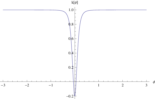
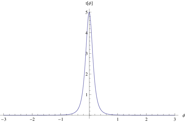
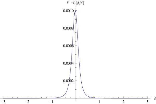
Furthermore, we would like to emphasize that by having the shapes of , and , one can successfully control each term such that the higher derivative term only dominates for a while in order to trigger the bounce, while disappears before and after that, not disturbing the evolution before and after the bounce. In fact, if we do not control the higher derivative term, it will usually become more and more important after dominance, leading to a very fast evolution of the universe instead of a modest one, or even the “big-rip” singularity. Moreover, using -like shape function, we can naturally connect and so that the field can evolve naturally from a lower potential to a higher one, leading to inflation. Therefore we can see that, shape functions are actually very useful in constructing models. We also show the shape functions and potential explicitly by numerics in Fig. 1 and 2. For pioneer works of using this shape functions to model building, see [29, 30] for ghost-free bounce and see [35] for dark energy models.

Now let’s go to a little bit more detail about the field evolution both before and after the bounce, which actually become very simple. In the contracting phase before the bounce when Eq. (8) applies, the equation of motion of becomes:
| (10) |
The energy density and pressure of thus becomes
| (11) |
while the EoS and the slow-roll parameter of the universe are
| (12) |
Since due to the requirement of positivity of the energy density, is obviously larger than unity, and the growth of the energy density will be larger than the anisotropy, avoiding the dominance of the latter. So the negative potential is rather useful in avoiding the cosmic anisotropy problem.
Setting the initial values of be negative, and once approaches 0 with certain amount of velocity , the higher derivative terms is turned on, which is responsible to trigger the bounce. After bounce however, as Eq. (9) applies, these terms decay away again, and one will have:
| (13) |
which gives the solution of inflation. According to the potential, one can express the slow-roll parameter as well as the e-folding number of the inflation as:
| (14) |
By requiring and , the field values at starting and ending points of inflation can be calculated as:
| (15) |
One can see again that the has monotonically increasing evolution. The potential has valley with a minimum at , and when falls down the valley, it will become oscillating rapidly, which reheats our universe. The whole evolution of the , , and are sketched in Fig. 3.


III perturbations
III.1 scalar perturbations
In this section, we analyze the perturbations that could be generated in this model. Following the general formulae for calculating perturbations of Galileon models in [36, 37], the 2-nd order perturbed lagrangian based on (1) turns out to be:
| (16) |
where
| (17) | |||||
| (18) |
Here is the variable of adiabatic perturbation, while is the sound speed squared of , representing how fast the perturbations can propagate. From the quantum field theories, the ghost-free condition of is . Moreover, the gradient stability requires . From Eqs. (17) and (18) one can see that, for most of the evolution when approximations (8) and (9) are reached, we have or and . However, for the region near the bounce, evolution are very complicated, and numerical calculations are required. Here we numerically plot and in Fig. 4.


From the Fig. 4 we can see that, in the whole evolution (including the bounce) we have positive , indicating that our model is completely ghost-free. However, during the bounce region, the numerics show that there is a instant period of negative , which may induce fast increase of the perturbations. We will later show what sequent it will cause to have negative and how it can be ameliorated. In fact, the same issue also appears in the model given by [29, 30]. Let’s first write down the equation of motion for according to lagrangian (16):
| (19) |
where
| (20) |
and “” and “” denotes derivatives with respect to conformal time and space respectively. When transformed into momentum space, one has for each wavenumber , and can be substituted into . According to the numerical result in the last section, we can plot the evolutions of fluctuation modes for different wavelengths as well as the Hubble horizon of our model as in Fig. 5. From the sketch plot one can see that, these fluctuation modes can been divided into two parts, one is of small ’s (green, cyan and blue), while the other is of large ’s (navy and purple). The former modes are generated in the contracting phase, and will exit the horizon before bouncing, while the latter ones are generated in expanding phase, and will exit the horizon after bouncing. As will be shown very soon, they will have very different evolution and -dependence. We remark the dividing mode between the two as (the blue one), the wavelength of which is just equal to horizon at the beginning of the bounce region.

III.1.1 initial condition
Since during the whole evolution, the background is different at each stage, and will lead to different evolution of perturbation. In the following subsections, we will analyze evolution in each stage separately, and joint them together using matching conditions to get the final power spectrum.
At far past, every mode is inside the horizon. In this region, we solve the Eq. (19) and taking the limit, and obtain the solution:
| (21) |
As we know that in contracting phase except near the bouncing phase, and can be approximated as . Moreover, the coefficient can be normalized by requiring a quantum origin of the perturbations [38]. We assume that the perturbations starts from Bunch-Davies vacuum as usual, and from the quantum condition, we have . So the initial condition for is:
| (22) |
III.1.2 contracting phase
In the most part of contracting phase, the model will be governed by the potential term while the higher derivative terms are severely suppressed. In this case, the approximation (8) applies, and from (17) and (18) one has and . Moreover, if the universe evolves according to the scaling solution of Eq. (10) with the EoS being as (12), the scale factor of the universe in contracting phase can be parameterized as
| (23) |
where , and and are the conformal time and conformal Hubble parameter at the end point of the contracting phase, respectively. The perturbation equation (19) then becomes
| (24) |
The solution of the above equation is Hankal function:
| (25) |
with the coefficients and to be determined by the initial conditions (22). Here
| (26) |
In the region far away from the bounce where all the fluctuation modes are deep inside the horizon, one have , and the solution (25) can be approximated as:
| (27) |
In the region near the bounce, the horizon shrinks rapidly to a minimum value. In this case, some fluctuation modes with small , namely will exit the horizon and become superhorizon modes in the contracting phase. The approximate behavior of these modes according to the solution (25) will be:
| (28) |
while the large mode still remains the same as (27).
The subhorizon solution in the contracting phase, which describes the modes deep inside the horizon, can be connected to the initial condition (22) to find out the coefficients and . Using (22) and (27) we will get:
| (29) |
One can see that while subhorizon modes shows oscillating behavior, the superhorizon modes splits into two branches, one keeps constant and the other is decaying. Assuming the two modes are generated equally, one could easily understood that for modes that exits horizon at contracting phase, the constant mode will dominate over the decaying one, and will be inherited by the perturbations through the bounce and in expanding phase. We will investigate the following evolution of perturbations in the coming sections.
III.1.3 through the bounce
After the Hubble parameter of the universe reaches the minimum value, it will no longer evolve as an monotonic function which keeps negative, but rather turns around towards positive values. This will cause the universe contract more and more slowly, while finally it stops contracting and becomes expanding, triggering the bounce. The Hubble parameter will go from its minimum value to its maximum value, the process during which we call as a bouncing phase. During the bouncing phase, the Hubble parameter is increasing rather than decreasing, and shape functions such as , and , as well as and , will have nontrivial features, which will make Eq. (19) hard to solve. For sake of analyticity, we assume that the Hubble parameter increases as:
| (30) |
when is the time point when the bounce happens. Then we have
| (31) |
for the scale factor. Here refers to the scale factor at . From the numerical calculation, it can be identified that around the bouncing point the first two terms of the Lagrangian (1) will be dominant, so one roughly have:
| (32) |
respectively. Using Friedmann equations, one can furtherly simplify to be
| (33) |
and near the bouncing point where the -dependent terms can be viewed as higher order. Moreover, near the bouncing point, the hubble parameter will be small compared to the term in the dominator of (at bouncing point ), where is obtained from in (6). From (6), one can notice that in our model , so can be expressed as
| (34) |
It is convenient to approximately parameterize X as function of [29]:
| (35) |
where is the parameter and is the value of at the bouncing point. From the numerical calculation we find that the parametrization can efficiently mimic the evolution of near the bouncing point.
It is convenient to transfer everything into conformal coordinate where the time is denoted by the conformal time . From the definition of one can see that for leading order , where is the conformal time at the bouncing point. Then from Eq. (32) one can express and w.r.t. approximately as:
| (36) |
and the parameter turns out to be:
| (37) |
Though insures there is no ghost instability, leads to a gradient instability, which mainly affects the small-scale perturbation modes. These small-scale modes are within the horizon, i.e. the wavelength (noting that the superhorizon modes are hardly affected, see [30].), in which case the perturbation modes present quantum-behavior. At classical level, it still remains an open issue of how to estimate the effect of this gradient instability. Here, we will not involve this issue in this paper, which is beyond our scope.
However, the nasty instability might be avoided if we expect some additional corrections in the high energy region such as around the bounce [42]. For example, we phenomenologically assume that there is an additional term in the action of gravity such as:
| (38) |
the physics of which is yet to be known, where the 3-metric can be viewed as the scalar component of potential term of the 4D gravity. In order not to affect gravity at other regions of evolution, is required to go close to zero at past or future limit but reach its extreme value at the bounce. Since as a spatial curvature, only, so this term will do nothing to the background evolution as well as the time derivative of , but will add another spatial derivative term of such as
| (39) |
so adding this term, the effective sound speed squared becomes:
| (40) |
In order to make around the bounce, we only need
| (41) |
which can be easily satisfied by choosing proper form of . As an example, we parameterize as , and plot the evolution of in Fig. 6. From the plot we can see that now the sound speed squared will be positive all the time, avoiding the gradient instability around the bounce, while reduce to the one in contracting phase due to the quick decay of far from the bounce.

The EoM of perturbation now becomes
| (42) |
with a positive . As explicit examples, we set , and while , and find that can be easily kept above zero (the minimum required value of is , which gives ). The solution is:
| (43) |
for any , where . In general, we have during bouncing phase, and this is the requirement of kinetic dominance in order to get a bounce: . This relation can also be numerically checked in our model.
The solution during bouncing phase should be matched onto the solution in contracting phase via the matching conditions. We apply the Hwang-Vishniac (Deruelle-Mukhanov) matching conditions [39, 40] that and its derivative should be matched at the pivot point (see also [41] for matching conditions in Galileon theories.). Using the solutions (27), (29) and (43) we have:
| (44) | |||||
for subhorizon modes while with (28), (29) and (43) we have:
| (45) |
for superhorizon modes.
III.1.4 expanding phase
After the bounce, the universe will enter into an inflationary expanding phase, with the Hubble parameter being a little bit decreasing but nearly steady. In this phase, all the features of the shape functions will decay again and make them the same constant value as before the bounce. Moreover, the parameters and will become constant again, with and . The scale factor during this time can be parameterized as:
| (46) |
while to protect the continuity of , and the slow-roll parameter is defined in Eq. (14). However, since during the most of the time is much smaller than the expectation value , one have and , thus it is reasonable to take as nearly a constant. Then the equation of motion (19) becomes:
| (47) |
and the solution is the Hankal function:
| (48) |
where
| (49) |
As has been discussed in the subsection 2, the solution of Eq. (48) also has two branches of solution. One is the subhorizon solution:
| (50) |
This solution is for the large modes, which still remains inside the horizon at least at the time when the universe enters the expanding phase. This branch should be matched with the large modes in bouncing phase (43). The other branch of the solution of (48) is the superhorizon solution:
| (51) |
This solution has two origins: one of the origin is from the large modes, which exit the horizon during the expanding phase. Since it shares the same equation with the subhorizon solution (50), the coefficients of the two parts will be the same. The other origin is from the small modes, which already exit the horizon when the universe enters the expanding phase. This solution should be matched with the small modes in bouncing phase (44). So we have:
| (52) | |||||
for those which exit the horizon in expanding phase, where we define , and
| (53) |
for those which exit the horizon before the bounce.
We are observing superhorizon modes, namely. For the solution of the superhorizon mode (51) which we’re observing, the constant branch will be dominant over the decaying branch . The power spectrum is then
| (54) |
Considering that , , the modulus squared of is calculated as:
| (55) | |||||
For large modes, the trigonometric functions in the above expression will oscillate rapidly, showing only their average values, which is zero. Then the mean value of .
One can see that, for modes that exit horizon before bounce,
| (56) |
with the index
| (57) |
Since , it will have a blue tilt.
While for modes that exit horizon after bounce, the power spectrum is in the form of:
| (58) |
and the spectral index
| (59) |
We can see that, taking the correction (38), it shows scale-invariance even at the limit, which is consistent with the data. When we take the slow-roll limit , we have . Moreover, if one also take into account the corrections from the trigonometric functions in , both and will have some wiggling behavior due to such a correction, which will be observed if we have enough accurate data. The same property has been discussed in the second paper of Ref. [11]. This property can be used to distinguish from the standard inflation models without preceding evolution.
III.2 tensor perturbations
Besides the scalar part, there are also tensor part perturbations. Since the field is pure scalar field and there are no tensor degrees of freedom in the field part, the tensor part totally come from the perturbations of the gravity. It is believed that the tensor perturbation is originated from the primordial gravitational waves, and although very weak, the recent gravitational wave explorers such as BICEP has shed some light on our future ability of detecting them more clearly [43]. As a theoretical study, here we also discuss the tensor perturbations generated in our model. According to [38], the equation of motion for tensor perturbations can be written as:
| (60) |
where is the amplitude of the spatial-spatial part perturbations of the metric, namely . There are two degrees of freedom in tensor parts, namely and , obeying the same action and equation of motion. From (60) we get the equation of motion for as:
| (61) |
where we define . From both the action and the equation of motion we can see that, the evolution of the tensor part will be affected only by the evolution of the universe itself, namely the scale factor , rather than the functions containing . This is due to that tensor part is decoupled from scalar part, and only comes from the gravity. Thus solving the equation of motion for tensor perturbations will be much easier than that for scalar ones.
We follow the same procedure as what we did in subsec. A. At the very beginning when all the modes are deep inside the horizon, the last term in the left hand side of Eq. (61) is not important, thus similar to scalar part, has the oscillating solution. For the initial condition of , we also choose the Bunch-Davies vacuum, so the tensor perturbation at the initial time have the solution as:
| (62) |
For contracting phase where we have , we have the solution for tensor perturbations as:
| (63) |
where is already given in Eq. (26). Since in this period the functions such as and for scalar perturbations also becomes trivial, the solution of tensor and scalar perturbations are actually very similar. For large modes which remains inside horizon during contraction phase, the solution is:
| (64) |
while for small modes which has already exit the horizon during contracting phase, the solution will be
| (65) |
By connecting the subhorizon solution with initial condition (62), one can get the coefficients:
| (66) |
For bouncing phase however, the tensor perturbation shows greatest difference with the scalar perturbations, for it is independent of functions such as and , which becomes nontrivial any more in bouncing phase. Considering Eq. (61) and the expression of scale factor in bouncing phase (31), the equation of motion for now becomes (in its leading order):
| (67) |
and the solution is:
| (68) | |||||
| (69) |
where . Note that will run from to , and the value of at is the amplitude growth of the tensor perturbations during bouncing period. Via matching conditions which requires continuity of and [39, 40], one can determine the coefficient as:
| (70) |
for subhorizon modes, while
| (71) |
for superhorizon modes.
In expanding phase, the tensor perturbations becomes concordance with the scalar ones again. Since the scale factor now becomes , the solution for becomes:
| (72) |
Also the solutions are divided by subhorizon and superhorizon parts. The subhorizon part is:
| (73) |
which denotes the modes that remains inside the horizon at the beginning of the expanding phase. While the superhorizon parts is:
| (74) |
which denotes the modes that are outside the horizon. These modes also have two origins. For those which exit the horizon in expanding phase, using matching conditions with the solution in (68) and (73), we have:
| (75) |
and for those which exit the horizon before the bounce, one obtain
| (76) |
Similar as the scalar part, we are observing superhorizon modes, namely (74). For this solution, it has two branches, one is constant () and the other is decaying , therefore the first one is dominant. The power spectrum is then
| (77) |
where the factor appears because there are 2 independent polarizations of the graviton [44]. One can see that, for modes that exit horizon in the inflation phase,
| (78) |
with the index . For , we have and . While for modes that exit horizon before bounce,
| (79) |
with the index . Since , it will have a blue tilt.
From the above result for scalar and tensor perturbations, we can also calculate the tensor-to-scalar ratio , defined as . The 1st year Planck paper suggest to have at level, while BICEP2 data shed some light on the possibility to measure it more accurately. In our model, we have
| (80) |
One can see that for large modes which is observable, carries information from bouncing or contracting phase, which makes bounce detectable. For example, the Planck constraint requires that for the minimum value of , which furtherly lead to for in the parametrization of . However, for small modes which has not been detectable yet, could be very large . This could be a smoking gun to the bounce inflation scenario.
As a side remark, we would like to comment that actually all the above analysis is based on the consideration that the bounce is not far from observable inflation, i.e. the e-fold number is not too much, so the information from the bounce can be detectable. However, there is also possibility that if the inflation was too long, therefore the observed modes comes from Bunch-Davies vacuum even in expanding time (like the purple line in the Fig. 5). In this case, we instead have , , so everything could be completely the same as pure inflation and bounce becomes non-detectable. As for in the region before the bounce, this mode should be inside quantum phase all the time, and solutions in different stages may be matched quantum mechanically. Of course such an issue goes far beyond the scope of this paper, and actually we don’t know how to do it yet. There may be chances that we pick up this topic in future investigations.
IV fitting the data
In this section, we try to fit our model with the newest released PLANCK data. Following (56) and (58), we parametrize the whole power spectrum as:
| (81) |
where and are the -independent prefactors of expressions (56) and (58), and and refers to Eqs. (57) and (59) respectively. According to this parametrization, we plot the CMB TT power spectrum of pure power-law inflation model and our model in Fig. 7. From the figure we can see that, in most of the plotted region () our model is identified with the inflation model, and fits the data very well. This is actually not strange, because the perturbations of observable scales exits the horizon during inflation era, and should carry information of inflation part. The tiny errorbars of the data in this region also indicate that the measurement has been done accurate enough, and the shape is almost confirmed and hardly to have other alternatives. However, the data at very large scales has large error bars, and the data is not so accurate. Moreover, the data points mildly favor that there is suppression in this region. In pure power-law inflation models where all the fluctuation modes are scale-invariant, it is difficult to obtain such an suppression, however, in our models where the fluctuation modes exit the horizon before bounce, suppression takes place due to the blue-tilt of the spectrum. This result is consistent with [23, 28], which could be seen as an important distinct from our model and inflation.

V Conclusion
Inflation theories, although has achieved great accomplishments, has actually been suffering from the singularity problem. Phenomenologically, considering a non-singular bounce happens before inflation can help avoid the singularity. The bounce indicates that prior to our expanding universe, the universe might have been contracting from a large volume. The bounce scenario not only provide an answer to the mysterious question of “what is our Universe like even before inflation”, but more scientifically, may bring some new features to the early stage of our Universe, and provide predictions that can be discovered in the future observations.
However, to add a bounce before inflation, one should care about whether it could bring new problems. To our knowledge, the ghost instability and the cosmic anisotropy problems are among the most serious problems of the bounce scenario. One is due to the NEC violation which is necessary for the bounce, and the other is due to the growth of anisotropy during contraction. In this paper, we present a model making use of the Galileon theory, which can violate the NEC and realize bounce behavior without introducing ghosts, because of the delicate design of the Lagrangian. Moreover, a negative potential in the contracting phase, which causes the EoS of this model large than unity, is useful to avoid the dominance of the cosmic anisotropy. In order to enter into the usual inflationary era after the bounce, the potential of the model will have to be connected to some positive value functions, which can be realized phenomenologically by shape functions.
Since now there are multi-stages in the evolution of the early universe, primordial perturbations can be generated in either in contracting phase or expanding phase. Those generated in expanding phase corresponds to large wavenumber (small scale), which has entered into horizon and can be observed by nowadays observations. Taking proper inflation potential, it is not difficult to get nearly scale-invariant with proper tilt, which is consistent with the PLANCK data. Meanwhile, those generated in contracting phase corresponds to small (large scale), which reenter into horizon much later, and can only be observed by future experiments. Due to the large background EoS in the contracting phase, the spectrum of these modes are blue-tilted, which will be more and more suppressed when the scales get larger and larger. However, there are already some hints in nowadays observation, i.e., the small suppression observed at TT spectra of CMB map. Moreover, the spectrum might present some oscillating features due to the bounce effect, and this can be viewed as a distinction to pure inflation models. Tensor perturbations and tensor spectrum are also discussed in this paper, which has similar behaviors as the scalar ones.
Nowadays along with the rapid development of the astrophysical observations, the observable range are getting more and more enlarged, and the observational data are also more and more accurate. More and more interesting new phenomena are discovered, which is not only chance but also challenge to the early universe model buildings. For instance, the newly released PLANCK data has pointed out that there have been several anomalies in the CMB sky, which has been stimulating great interests among astrophysicists and cosmologists. Can the bounce inflation scenario be good enough to explain those phenomena? Or what more phenomena can it predict that could be discovered by the future observations? We are trying to answer these questions in our upcoming works.
Acknowledgements.
We thank Jean-Luc Lehners and Yun-Song Piao for useful discussion. The work of T.Q. is supported in part by the Open Project Program of State Key Laboratory of Theoretical Physics, Institute of Theoretical Physics, Chinese Academy of Sciences, China (No.Y4KF131CJ1), and in part by NSFC under Grant No: 11405069. The work of Y.T.W. is supported in part by NSFC under Grant No:11222546, in part by National Basic Research Program of China, No:2010CB832804.References
- [1] A. H. Guth, Phys. Rev. D 23, 347 (1981).
- [2] A. D. Linde, Phys. Lett. B 108, 389 (1982).
- [3] A. Albrecht and P. J. Steinhardt, Phys. Rev. Lett. 48, 1220 (1982).
- [4] A. A. Starobinsky, Phys. Lett. B 91, 99 (1980).
- [5] L. Z. Fang, Phys. Lett. B 95, 154 (1980).
- [6] K. Sato, Mon. Not. Roy. Astron. Soc. 195, 467 (1981).
- [7] S. W. Hawking and R. Penrose, Proc. Roy. Soc. Lond. A 314, 529 (1970); S. W. Hawking and G. F. R. Ellis, Cambridge University Press, Cambridge, 1973.
- [8] A. Borde and A. Vilenkin, Phys. Rev. Lett. 72, 3305 (1994) [gr-qc/9312022].
- [9] M. Novello and S. E. P. Bergliaffa, Phys. Rept. 463, 127 (2008) [arXiv:0802.1634 [astro-ph]].
- [10] Y. -F. Cai, T. Qiu, Y. -S. Piao, M. Li and X. Zhang, JHEP 0710, 071 (2007) [arXiv:0704.1090 [gr-qc]].
- [11] Y. -F. Cai, T. Qiu, R. Brandenberger, Y. -S. Piao and X. Zhang, JCAP 0803, 013 (2008) [arXiv:0711.2187 [hep-th]]; Y. -F. Cai, T. -t. Qiu, J. -Q. Xia and X. Zhang, Phys. Rev. D 79, 021303 (2009) [arXiv:0808.0819 [astro-ph]]; Y. -F. Cai, T. -t. Qiu, R. Brandenberger and X. -m. Zhang, Phys. Rev. D 80, 023511 (2009) [arXiv:0810.4677 [hep-th]]; T. Qiu and K. -C. Yang, JCAP 1011, 012 (2010) [arXiv:1007.2571 [astro-ph.CO]].
- [12] H. -H. Xiong, T. Qiu, Y. -F. Cai and X. Zhang, Mod. Phys. Lett. A 24, 1237 (2009) [arXiv:0711.4469 [hep-th]]; H. -H. Xiong, Y. -F. Cai, T. Qiu, Y. -S. Piao and X. Zhang, Phys. Lett. B 666, 212 (2008) [arXiv:0805.0413 [astro-ph]].
- [13] Y. -S. Piao, Phys. Rev. D 70, 101302 (2004) [hep-th/0407258]; Y. -S. Piao, Phys. Lett. B 677, 1 (2009) [arXiv:0901.2644 [gr-qc]]; J. Zhang, Z. -G. Liu and Y. -S. Piao, Phys. Rev. D 82, 123505 (2010) [arXiv:1007.2498 [hep-th]].
- [14] M. Ostrogradski, Mem. Ac. St. Petersbourg VI 4, 385 (1850); R. P. Woodard, Lect. Notes Phys. 720, 403 (2007) [astro-ph/0601672].
- [15] S. M. Carroll, M. Hoffman and M. Trodden, Phys. Rev. D 68, 023509 (2003) [astro-ph/0301273]; J. M. Cline, S. Jeon and G. D. Moore, Phys. Rev. D 70, 043543 (2004) [hep-ph/0311312].
- [16] V. K. Onemli and R. P. Woodard, Class. Quant. Grav. 19, 4607 (2002) [gr-qc/0204065]; V. K. Onemli and R. P. Woodard, Phys. Rev. D 70, 107301 (2004) [gr-qc/0406098]; E. O. Kahya and V. K. Onemli, Phys. Rev. D 76, 043512 (2007) [gr-qc/0612026].
- [17] A. Nicolis, R. Rattazzi and E. Trincherini, Phys. Rev. D 79, 064036 (2009) [arXiv:0811.2197 [hep-th]]; C. Deffayet, G. Esposito-Farese and A. Vikman, Phys. Rev. D 79, 084003 (2009) [arXiv:0901.1314 [hep-th]]; A. Nicolis, R. Rattazzi and E. Trincherini, JHEP 1005, 095 (2010) [Erratum-ibid. 1111, 128 (2011)] [arXiv:0912.4258 [hep-th]].
- [18] C. Deffayet, S. Deser and G. Esposito-Farese, Phys. Rev. D 80, 064015 (2009) [arXiv:0906.1967 [gr-qc]]; C. Deffayet, X. Gao, D. A. Steer and G. Zahariade, Phys. Rev. D 84, 064039 (2011) [arXiv:1103.3260 [hep-th]].
- [19] G. W. Horndeski, Int. J. Theor. Phys. 10, 363 (1974).
- [20] T. Qiu, J. Evslin, Y. -F. Cai, M. Li and X. Zhang, JCAP 1110, 036 (2011) [arXiv:1108.0593 [hep-th]]; D. A. Easson, I. Sawicki and A. Vikman, JCAP 1111, 021 (2011) [arXiv:1109.1047 [hep-th]].
- [21] T. Qiu, X. Gao and E. N. Saridakis, Phys. Rev. D 88, no. 4, 043525 (2013) [arXiv:1303.2372 [astro-ph.CO]].
- [22] K. E. Kunze and R. Durrer, Class. Quant. Grav. 17, 2597 (2000) [arXiv:gr-qc/9912081]; J. K. Erickson, D. H. Wesley, P. J. Steinhardt and N. Turok, Phys. Rev. D 69, 063514 (2004) [arXiv:hep-th/0312009]; B. Xue and P. J. Steinhardt, Phys. Rev. Lett. 105, 261301 (2010) [arXiv:1007.2875 [hep-th]]; B. Xue and P. J. Steinhardt, Phys. Rev. D 84, 083520 (2011) [arXiv:1106.1416 [hep-th]].
- [23] Y. -S. Piao, B. Feng and X. -m. Zhang, Phys. Rev. D 69, 103520 (2004) [hep-th/0310206]; Y. -S. Piao, Phys. Rev. D 71, 087301 (2005) [astro-ph/0502343]; Y. -S. Piao, S. Tsujikawa and X. -m. Zhang, Class. Quant. Grav. 21, 4455 (2004) [hep-th/0312139].
- [24] T. Qiu, arXiv:1404.3060 [gr-qc].
- [25] Z. G. Liu, Z. K. Guo and Y. S. Piao, Phys. Rev. D 88, 063539 (2013) [arXiv:1304.6527].
- [26] Y. T. Wang and Y. S. Piao, Phys. Lett. B 741, 55 (2015) [arXiv:1409.7153 [gr-qc]].
- [27] J. Q. Xia, Y. F. Cai, H. Li and X. Zhang, Phys. Rev. Lett. 112, 251301 (2014) [arXiv:1403.7623 [astro-ph.CO]].
- [28] Y. Cai, Y. T. Wang and Y. S. Piao, arXiv:1501.01730 [astro-ph.CO].
- [29] Y. -F. Cai, D. A. Easson and R. Brandenberger, JCAP 1208, 020 (2012) [arXiv:1206.2382 [hep-th]].
- [30] M. Koehn, J. L. Lehners and B. A. Ovrut, Phys. Rev. D 90, 025005 (2014) [arXiv:1310.7577 [hep-th]]; L. Battarra, M. Koehn, J. L. Lehners and B. A. Ovrut, JCAP 1407, 007 (2014) [arXiv:1404.5067 [hep-th]].
- [31] J. Khoury, B. A. Ovrut, P. J. Steinhardt and N. Turok, Phys. Rev. D 64, 123522 (2001) [arXiv:hep-th/0103239]; J. Khoury, B. A. Ovrut, N. Seiberg, P. J. Steinhardt and N. Turok, Phys. Rev. D 65, 086007 (2002) [arXiv:hep-th/0108187]; J. Khoury, B. A. Ovrut, P. J. Steinhardt and N. Turok, Phys. Rev. D 66, 046005 (2002) [arXiv:hep-th/0109050].
- [32] A. Fertig, J. L. Lehners and E. Mallwitz, Phys. Rev. D 89, 103537 (2014) [arXiv:1310.8133 [hep-th]]; A. Ijjas, J. L. Lehners and P. J. Steinhardt, PhysRevD 89 (2014) 123520 [arXiv:1404.1265 [astro-ph.CO]].
- [33] K. A. Olive, Phys. Rept. 190, 307 (1990).
- [34] P. A. R. Ade et al. [Planck Collaboration], arXiv:1303.5082 [astro-ph.CO].
- [35] X. F. Zhang and T. Qiu, Phys. Lett. B 642, 187 (2006) [astro-ph/0603824].
- [36] T. Kobayashi, M. Yamaguchi and J. ’i. Yokoyama, Phys. Rev. Lett. 105, 231302 (2010) [arXiv:1008.0603 [hep-th]].
- [37] A. De Felice and S. Tsujikawa, Phys. Rev. D 84, 083504 (2011) [arXiv:1107.3917 [gr-qc]].
- [38] V. F. Mukhanov, H. A. Feldman and R. H. Brandenberger, Phys. Rept. 215, 203 (1992).
- [39] J. c. Hwang and E. T. Vishniac, Astrophys. J. 382, 363 (1991).
- [40] N. Deruelle and V. F. Mukhanov, Phys. Rev. D 52, 5549 (1995) [arXiv:gr-qc/9503050].
- [41] S. Nishi, T. Kobayashi, N. Tanahashi and M. Yamaguchi, JCAP 1403, 008 (2014) [arXiv:1401.1045 [hep-th]].
- [42] D. Pirtskhalava, L. Santoni, E. Trincherini and P. Uttayarat, arXiv:1410.0882 [hep-th].
- [43] P. A. R. Ade et al. [BICEP2 Collaboration], arXiv:1403.3985 [astro-ph.CO].
- [44] B. A. Bassett, S. Tsujikawa and D. Wands, Rev. Mod. Phys. 78, 537 (2006) [astro-ph/0507632].