Vacuum stability of asymptotically safe gauge-Yukawa theories

Following [1], we consider a massless quantum field theory with $SU(N_{C})$ gauge fields $A^{a}_{\mu}$ and field strength $F^{a}_{\mu\nu}$ $(a=1,\cdots,N^{2}_{C}-1)$, $N_{F}$ flavors of fermions $Q_{i}$ $(i=1,\cdots,N_{F})$ in the fundamental representation, and a $N_{F}\times N_{F}$ complex matrix scalar field $H$ invariant under $U(N_{F})_{L}\times U(N_{F})_{R}$ rotations and uncharged under the gauge group. The fundamental Lagrangian is given by the sum of the Yang-Mills term, the fermion and scalar kinetic terms, the Yukawa interaction, and scalar self-interaction terms,

	$\displaystyle L$	$\displaystyle=$	$\displaystyle-\mbox{\small{$\frac{1}{2}$}}{\rm Tr}\,F^{\mu\nu}F_{\mu\nu}+{\rm Tr}\left(\overline{Q}\,i\not{D}\,Q\right)+{\rm Tr}\,(\partial_{\mu}H^{\dagger}\,\partial^{\mu}H)$		(1)
			$\displaystyle+y\,{\rm Tr}\left(\overline{Q}_{L}HQ_{R}+\overline{Q}_{R}H^{\dagger}Q_{L}\right)-u\,{\rm Tr}\,(H^{\dagger}H)^{2}-v\,({\rm Tr}\,H^{\dagger}H)^{2}\,,$

where the decomposition $Q=Q_{L}+Q_{R}$ with $Q_{L/R}=\frac{1}{2}(1\pm\gamma_{5})Q$ is understood. The trace ${\rm Tr}$ indicates the trace over both color and flavor indices. The model has four classically marginal coupling constants in four space-time dimensions given by the gauge coupling $g$, the Yukawa coupling $y$, the quartic scalar couplings $h$ and the ‘double-trace’ scalar coupling $v$, which we write as

$$\alpha_{g}=\frac{g^{2}\,N_{C}}{(4\pi)^{2}}\,,\quad\alpha_{y}=\frac{y^{2}\,N_{C}}{(4\pi)^{2}}\,,\quad\alpha_{h}=\frac{{u}\,N_{F}}{(4\pi)^{2}}\,,\quad\alpha_{v}=\frac{{v}\,N^{2}_{F}}{(4\pi)^{2}}\,.$$

(2)

We have also added the appropriate powers of $N_{C}$ and $N_{F}$ in the normalization of the couplings. The shorthand notation $\beta_{i}\equiv\partial_{t}\alpha_{i}$ with $i=(g,y,h,v)$ is employed to indicate the $\beta$-functions for the couplings (2). In the Veneziano limit where both $N_{C}$ and $N_{F}$ are large but their ratio fixed, the parameter

$$\epsilon=\frac{N_{F}}{N_{C}}-\frac{11}{2}$$

(3)

can take any real value. In the large-$N$ limit, the perturbative renormalisation group equations for the couplings (2) have been obtained in [12] in dimensional regularisation, also using the results [13, 14, 15]. In terms of (3) they are given by

	$\displaystyle\beta_{g}$	$\displaystyle=$	$\displaystyle\frac{4}{3}\epsilon\,\alpha_{g}^{2}+\left\{\left(25+\frac{26}{3}\epsilon\right)\alpha_{g}-2\left(\frac{11}{2}+\epsilon\right)^{2}\alpha_{y}\right\}\alpha_{g}^{2}$		(4)
			$\displaystyle+\left\{\left(\frac{701}{6}+\frac{53}{3}\epsilon-\frac{112}{27}\epsilon^{2}\right)\alpha_{g}^{2}-\frac{27}{8}(11+2\epsilon)^{2}\alpha_{g}\alpha_{y}+\frac{1}{4}(11+2\epsilon)^{2}(20+3\epsilon)\alpha_{y}^{2}\right\}\alpha_{g}^{2}$
	$\displaystyle\beta_{y}$	$\displaystyle=$	$\displaystyle\alpha_{y}\,\Big\{(13+2\epsilon)\,\alpha_{y}-6\,\alpha_{g}\Big\}$		(5)
			$\displaystyle+\alpha_{y}\left\{\frac{20\epsilon-93}{6}\alpha_{g}^{2}+(49+8\epsilon)\alpha_{g}\alpha_{y}-\left(\frac{385}{8}+\frac{23}{2}\epsilon+\frac{\epsilon^{2}}{2}\right)\alpha_{y}^{2}-(44+8\epsilon)\alpha_{y}\alpha_{h}+4\alpha_{h}^{2}\right\}$
	$\displaystyle\beta_{h}$	$\displaystyle=$	$\displaystyle-(11+2\epsilon)\,\alpha_{y}^{2}+4\alpha_{h}(\alpha_{y}+2\alpha_{h})\,,$		(6)
	$\displaystyle\beta_{v}$	$\displaystyle=$	$\displaystyle 12\alpha_{h}^{2}+4\alpha_{v}\left(\alpha_{v}+4\alpha_{h}+\alpha_{y}\right)\,.$		(7)

for $\beta_{g},\beta_{y},\beta_{h}$ and $\beta_{v}$ up to $(3,2,1,1)$-loop order, respectively. In the terminology of [1] we refer to this as the next-to-next-to-leading order (NNLO) approximation. The NLO approximation corresponds to the approximation in which the $(2,1,0,0)$-loop terms for $\beta_{g},\beta_{y},\beta_{h}$ and $\beta_{v}$ are retained. As discussed in [1], this ordering of perturbation theory is also favoured by Weyl consistency conditions [16, 12, 17]. Additionally, we consider the NLO^′ approximation in which the $(2,1,1,1)$-loop terms are retained (see Tab. 1). We stress that the dynamics of the scalar couplings, central for our study of vacuum stability, arises for the first time within the NLO^′ and NNLO approximations.

The theory (1) is renormalisable within perturbation theory. For $\epsilon<0$ it also displays asymptotic freedom in the gauge sector. When $\epsilon$ is positive, asymptotic freedom is lost and the gauge sector becomes QED-like. In [1], it has been established that the theory (1) develops an exact, interacting UV fixed point in all four couplings, strictly controlled by perturbation theory, provided the parameter (3) is chosen to be

$$0<\epsilon\ll 1\,.$$

(8)

The existence of an interacting UV fixed point ensures that the theory (1) remains predictive to highest energies at the fixed point. Another feature of this theory is that the scalar sector avoids a triviality bound due to residual interactions in the UV, meaning that the scalars can be viewed as elementary.

In [1], it has been shown that the gauge-matter system (4) – (7) may display three different ultraviolet fixed points in the regime (8). In an expansion in the small parameter $\epsilon$, the first fixed point has the coordinates

$$\begin{array}[]{rcl}\alpha_{g}^{*}&=&\frac{26}{57}\,\epsilon+\frac{23(75245-13068\sqrt{23})}{370386}\,\epsilon^{2}+{\cal O}(\epsilon^{3})\\[4.30554pt] \alpha_{y}^{*}&=&\frac{4}{19}\,\epsilon+\left(\frac{43549}{20577}-\frac{2300\sqrt{23}}{6859}\right)\,\epsilon^{2}+{\cal O}(\epsilon^{3})\\[4.30554pt] \alpha_{h}^{*}&=&\frac{\sqrt{23}-1}{19}\,\epsilon+{\cal O}(\epsilon^{2})\,,\\[4.30554pt] \alpha_{v1}^{*}&=&-\frac{1}{19}(2\sqrt{23}-\sqrt{20+6\sqrt{23}})\,\epsilon+{\cal O}(\epsilon^{2})\,.\end{array}$$

(9)

We refer to the fixed point (9) as FP₁. There are two more fixed points in the perturbative domain (8), a second fully interacting fixed point FP₂ and a partial fixed point FP₃. The coordinates of FP₂ differ from FP₁ in (9) in the coordinate $\alpha_{v}$, whose fixed point becomes

$$\begin{array}[]{rcl}\alpha_{v2}^{*}&=&-\frac{1}{19}(2\sqrt{23}+\sqrt{20+6\sqrt{23}})\epsilon+{\cal O}(\epsilon^{2})\end{array}$$

(10)

instead. The second fixed point comes about because the double trace coupling does not couple to the RG flow of $(\alpha_{g},\alpha_{y},\alpha_{h})$, and its own RG flow (7) is quadratic in $\alpha_{v}$ to all orders in $1/N_{F}$ and $1/N_{C}$. Therefore, $\alpha_{v}$ may even interpolate between these two fixed points without affecting the fixed point for $(\alpha_{g},\alpha_{y},\alpha_{h})$.

Finally, a partial fixed point FP₃ arises where all but the double-trace coupling $\alpha_{v}$ settle onto a fixed point within the perturbative domain. The double-trace coupling continues to evolve logarithmically towards a perturbative Landau pole. Furthermore, $\alpha_{h}$ settles at a negative fixed point value while $\alpha_{g}^{*}$ and $\alpha_{y}^{*}$ remain equal to their values at (9) to this order in $\epsilon$. Towards UV momentum scales, the partial fixed point FP₃ is then characterised by

$$\begin{array}[]{rcl}\alpha^{*}_{h2}&=&\displaystyle-(\sqrt{23}+1)\ \frac{\epsilon}{19}+{\cal O}(\epsilon^{2})\\[8.61108pt] \alpha_{v}(\mu)&=&\displaystyle\alpha_{v}(\mu_{0})+\frac{\epsilon}{4}\,\kappa\tan\left(\kappa\,\epsilon\ln\frac{\mu}{\mu_{0}}\right)\end{array}$$

(11)

where $\kappa=\frac{4}{19}\sqrt{6\sqrt{23}-20}\approx 0.624$. We have chosen the scale $\mu_{0}$ as a free parameter with $\alpha_{v}(\mu_{0})=(2\,\epsilon\,\sqrt{23})/19\approx 0.505\,\epsilon$. The running for $\alpha_{v}$ in (11) is an exact solution of its beta function (7) provided that $\alpha_{g}$, $\alpha_{y}$ and $\alpha_{h}$ have settled on FP₃ to leading order in $\epsilon$. From (11) we observe that $\alpha_{v}$ reaches its perturbative UV Landau pole at

$$\Lambda_{\rm Landau}\approx\mu_{0}\,\exp\frac{\pi}{2\,\kappa\,\epsilon}\gg\mu_{0}\,.$$

(12)

A similar Landau pole is reached towards low energies.

In [1], the phase diagram of the model has been discussed at NLO accuracy. Here we extend the study to NLO^′ and NNLO order including effects due to the running scalar couplings, and illustrate results in Figs. 1, 2 and 3 which show portions of the phase diagram in the vicinity of the UV and IR fixed points.

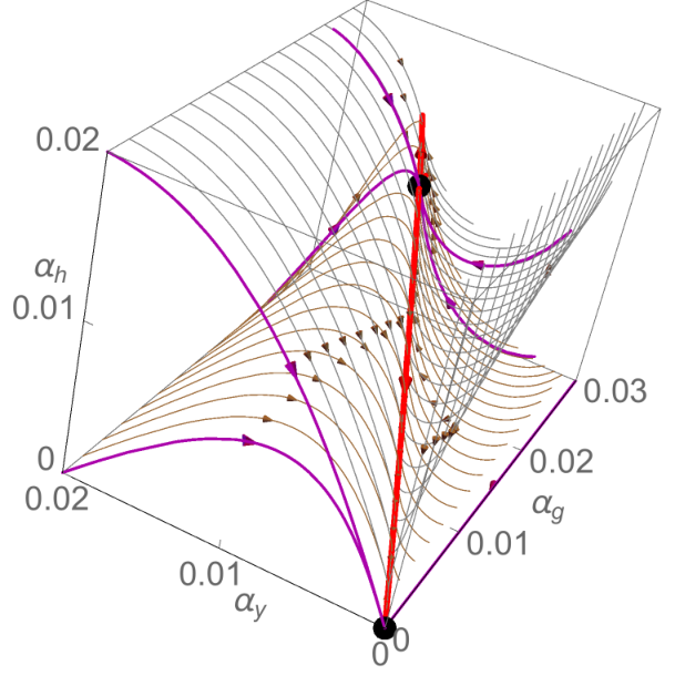
Specifically, Fig. 1 shows the RG trajectories for the couplings $(\alpha_{g},\alpha_{y},\alpha_{h})$, including the UV and IR fixed points and the UV-complete trajectory (thick red line) connecting them. It corresponds to a weakly coupled theory in the IR limit. The second UV complete trajectory runs towards large couplings, leading to a strongly coupled low energy theory with chiral symmetry breaking or conformality in the IR. The thin (magenta) trajectories emanating out of the UV stable fixed point correspond to the two irrelevant eigendirections of the fixed point. The other (thin magenta) trajectories illustrate that the Gaussian fixed point is an infrared fixed point for all couplings. Unlike in asymptotically free theories, it does not qualify as a UV fixed point. Finally, the thin (gray) lines show same trajectories which do not originate from a perturbative UV fixed point, but which nevertheless lead to a well-behaved weakly coupled theory at low energies.

Figs. 2 show the projection of Fig. 1 onto the $(\alpha_{g},\alpha_{y})$ and the $(\alpha_{g},\alpha_{h})$ plane, respectively. Notice the near-perpendicular behaviour of trajectories close to the separatrix in the $(\alpha_{g},\alpha_{y})$ plane (left panel). This is due to the fact that the velocity $\mu\partial_{\mu}$ of the RG flow of couplings along the separatrix is slower by an order in $\epsilon\ll 1$. In the range of parameters considered here, the RG flow has a velocity of order $\epsilon$ set by the Yukawa and scalar quartic couplings, yet the flow of the gauge coupling is smaller by a power in $\epsilon$. However, as soon as couplings are very close to the UV-IR connecting trajectory, the flow velocity becomes of order $\epsilon^{2}$ for all couplings, controlled by the gauge coupling. This effect is even more pronounced in the $(\alpha_{g},\alpha_{h})$ plane (right panel), because the scalar and gauge $\beta$-function are independent of each other at NNLO order. Consequently, the larger RG velocity of the scalar coupling becomes visible in the entire phase diagram, except along the separatrix. This effect plays also a rôle in the scalar subsector $(\alpha_{h},\alpha_{v})$ for which two snapshots are shown in Fig. 3. Here, the gauge and Yukawa couplings have been given values on the UV-IR connecting separatrix. Specifically, we have taken $\alpha_{g}\approx 0.999\,\alpha_{g}^{*}$ (left panel) and $\alpha_{g}\approx 0.397\,\alpha_{g}^{*}$ (right panel), respectively, and $\alpha_{y}$ determined via (15). Once again, in these projections, the RG flows in the scalar subsector have velocities of order $\epsilon$, whereas the flow velocity along the separatrix is of order $\epsilon^{2}$ and hence parametrically slower. Therefore the separatrix appears as a “pseudo” fixed point in this projection, indicated by a red dot. All other trajectories are attracted towards the separatrix. We also observe a second “pseudo” fixed point, indicated by a black dot. It relates to the trajectory which connects FP₂ with the Gaussian fixed point. However, along this trajectory the scalar field potential is unbounded from below and the theory is not considered to be physical.

Trajectories which emanate out of the UV stable fixed point correspond to finite theories at high energies. In the present case, the set of UV stable trajectories, sometimes denoted as the “UV critical surface”, is found to be one-dimensional [1]. The reason for this is a strictly dynamical one: the fluctuations at the UV fixed point are such that only one linear combination of the four classically marginal couplings (2) becomes quantum-mechanically relevant. Similar dynamical constraints can also arise for theories with “complete asymptotic freedom” [8]. More specifically, here, the one-dimensional critical surface leads to two UV safe trajectories. As indicated earlier, in the low-energy limit, they correspond to a weakly interacting theory of gluons, fermions and scalars with Gaussian scaling, and a strongly interacting theory with confinement, chiral symmetry breaking, or conformality.

The separatrix connects the UV fixed point with the Gaussian one. It coincides with the UV critical surface close to the fixed point [1], and is characterised by global aspects of the phase diagram, namely the location of its fixed points and the eigendirections. Therefore, in general, identifying a separatrix requires global information about the phase diagram. For generic values of the parameter $\epsilon$, the separatrix can always be found numerically. For some considerations, it is useful to have explicit analytical expressions for the UV-IR connecting trajectory. Here, we explain how an analytical expression for the separatrix can be obtained locally to leading order in $\epsilon\ll 1$ using the following observations. For small $\epsilon\ll 1$, the four eigenvalues at the UV fixed point are given by

$$\begin{array}[]{rcl}\vartheta_{1}&=&-\frac{104}{171}\,\epsilon^{2}+{\cal O}(\epsilon^{3})\\[8.61108pt] \vartheta_{2}&=&\ \ \,\frac{52}{19}\,\epsilon+{\cal O}(\epsilon^{2})\\[8.61108pt] \vartheta_{3}&=&\ \ \frac{16\sqrt{23}}{19}\,\epsilon+{\cal O}(\epsilon^{2})\\[8.61108pt] \vartheta_{4}&=&\ \ \frac{8}{19}\sqrt{20+6\sqrt{23}}\,\epsilon+{\cal O}(\epsilon^{2})\,.\end{array}$$

(13)

We note that the irrelevant (positive) eigenvalues are of order $\epsilon$ whereas the relevant (negative) eigenvalue is of order $\epsilon^{2}$. In consequence, the velocity $\mu\partial_{\mu}$ of the RG evolution of couplings along the separatrix is $\propto\epsilon^{2}$, whereas the velocity of the RG evolution towards the separatrix is $\propto\epsilon$. In the regime (8) we conclude that the approach towards the separatrix is substantially faster than the evolution along the separatrix. For fixed $\alpha_{g}$, this means that the corresponding value for the Yukawa coupling $\alpha_{y}$ on the separatrix can be found by solving $\beta_{y}=0$, to leading order in $\epsilon$. Following the same reasoning, for given $(\alpha_{g},\alpha_{y}$) on the separatrix, the corresponding value for $\alpha_{h}$ is then found from solving $\beta_{h}=0$. Finally, $\alpha_{v}$ follows from solving $\beta_{v}=0$ after inserting $(\alpha_{y},\alpha_{h}$) on the separatrix. Following this logic, we are led to solve

$$\begin{array}[]{rcl}\beta_{y}&=&0\,,\\ \beta_{h}&=&0\,,\\ \beta_{v}&=&0\end{array}$$

(14)

for $(\alpha_{y},\alpha_{h},\alpha_{v})$ in terms of $\alpha_{g}$ and to leading order in $\epsilon$. This leads to the following relations amongst couplings along the UV stable trajectories

$$\begin{array}[]{rcl}\alpha_{y}&=&\frac{6}{13}\,\alpha_{g}\ ,\\[8.61108pt] \alpha_{h}&=&\frac{3}{26}(\sqrt{23}-1)\,\alpha_{g}\ ,\\[8.61108pt] \alpha_{v}&=&\frac{3}{26}(\sqrt{20+6\sqrt{23}}-2\sqrt{23})\,\alpha_{g}\,.\end{array}$$

(15)

These relations for the separatrices are accurate in the limit $\epsilon\to 0$ (8). It remains to specify the RG running of the gauge coupling.

We now exploit the condition (14) to find the effective RG running of the gauge coupling along the separatrices. To simplify some of the subsequent expressions, we introduce $\alpha\equiv\alpha_{g}$ throughout this section. Its RG flow is given by

$$\partial_{t}\,\alpha=-B\,\alpha^{2}+C\,\alpha^{3}+{\cal O}(\alpha^{4})\,.$$

(16)

Below we will derive exact results valid for theories with (16) and generic $B,C\neq 0$. For the theory at hand, we concentrate on parameters in the regime $B<0$ and $C<0$ which take the specific values

$$\begin{array}[]{rcl}B&=&\displaystyle-\frac{4}{3}\epsilon\\[6.45831pt] C&=&\displaystyle-\frac{2}{3}\,\frac{57-46\epsilon-8\epsilon^{2}}{13+\epsilon}\,.\end{array}$$

(17)

They arise from (4) by expressing all $\alpha_{i}$ $(i=y,h,v)$ in terms of $\alpha$, which are found by solving each of (14) to one-loop accuracy. Evidently, the effective gauge $\beta$-function along the separatrix (16) displays three fixed points, a doubly-degenerated one at $\alpha_{*}=0$, and an interacting one at

$$\alpha_{*}=B/C>0\,.$$

(18)

Notice that in the absence of scalar fields and Yukawa interactions the coefficient $C$ would read $C=25>0$, and consequently the gauge coupling would not aquire an interacting UV fixed point in the physical domain $\alpha>0$. Including Yukawa interactions, the non-trivial fixed point is perturbative as long as $0\leq\alpha_{*}\ll 1$. In terms of (18), the solution to (16) is

$$\left(\frac{\mu}{\mu_{0}}\right)^{-B\cdot\alpha_{*}}=\left(\frac{\alpha_{*}-\alpha_{0}}{\alpha_{*}-\alpha}\cdot\frac{\alpha}{\alpha_{0}}\right)\exp\left(\frac{\alpha_{*}}{\alpha_{0}}-\frac{\alpha_{*}}{\alpha}\right)$$

(19)

Here, $-B\cdot\alpha_{*}>0$, and $\alpha\equiv\alpha(\mu)$ denotes the running gauge coupling along the separatrix, $\mu_{0}$ the initial scale, and $\alpha_{0}\equiv\alpha(\mu=\mu_{0})$ the gauge coupling at that scale. The solution (19) provides a closed expression for $\mu=\mu(\alpha)$. One easily confirms that (19) interpolates between the UV and IR fixed points. For $\alpha\to 0$ the exponential term dominates, thereby showing that it corresponds to an IR fixed point with $\mu\to 0$. In return, $\alpha\to\alpha_{*}$ corresponds to the UV limit where the algebraic term in (19) dominates, $\mu\to\infty$, and we recognize the appearance of the scaling exponent $\vartheta_{1}=B\cdot\alpha_{*}$. Note that if $\alpha_{0}>\alpha_{*}$ the Gaussian fixed point cannot be reached. Rather, RG trajectories then evolve towards strong coupling for all scales $\mu<\mu_{0}$. In order to invert the solution $\mu=\mu(\alpha)$ into $\alpha=\alpha(\mu)$ we introduce

	$\displaystyle W$	$\displaystyle=$	$\displaystyle\frac{\alpha_{*}}{\alpha}-1$		(20)
	$\displaystyle z$	$\displaystyle=$	$\displaystyle\left(\frac{\mu_{0}}{\mu}\right)^{-B\cdot\alpha_{*}}\left(\frac{\alpha_{*}}{\alpha_{0}}-1\right)\exp\left(\frac{\alpha_{*}}{\alpha_{0}}-1\right)\,.$		(21)

For $\mu/\mu_{0}$ ranging between $[0,\infty]$ and $0<\alpha_{0}<\alpha_{*}$, we have that both $z$ and $W$ interpolate monotonously between $[\infty,0]$. For $0<\alpha_{*}<\alpha_{0}$, we have that $z$ becomes negative. Using these expressions, (19) turns into

$$z=W\exp W$$

(22)

whose solution $W=W[z]$ is given by Lambert’s $W$ function. Uniqueness is observed provided that $z\geq 0$, which always holds true for the separatrix towards the Gaussian. In this regime the Lambert W function is monotonically increasing, polynomially so for small $z$ and approaching $\ln z$ from below for large $z$. For negative $z$, the Lambert W function is multivalued. The relevant branch is then the one with $W[z]\to 0$ for $z\to 0$.

In terms of (20) and (21), the fully resolved solution is finally written as

$$\alpha(\mu)=\frac{\alpha_{*}}{1+W(\mu)}\ ,$$

(23)

where we introduced the shorthand notation $W(\mu)\equiv W[z(\mu)]$ with $W[z]$ the Lambert function, and $z(\mu)$ given in (21). Together with (15), the solution (23) fully describes the RG evolution of couplings along the separatrix to leading order in $\epsilon$.

The dynamics of the theory towards low energies is characterised by an energy scale $\Lambda_{c}$ where the RG flow displays a cross-over from UV fixed point scaling to either Gaussian scaling, or strong coupling, in the IR. The scale $\Lambda_{c}$ arises dynamically through the mechanism of “dimensional transmutation”, and its rôle is similar to that of $\Lambda_{\rm QCD}$ for QCD. To identify the characteristic energy scale $\Lambda_{c}$, we use(16) or (19) to introduce the effective scaling exponent $\vartheta(\alpha)=\left.\partial_{\alpha}\beta_{g}\right|_{\rm sep}$ which reads

$$\vartheta(\alpha)=-2B\,\alpha\,\left(1-\frac{3}{2}\frac{\alpha}{\alpha_{*}}\right)\,.$$

(24)

Close to the UV and IR fixed points, $\vartheta$ reduces to the conventional scaling exponents

$$\begin{array}[]{lcl}\vartheta(\alpha\to 0)&=&-2\cdot B\cdot\alpha\to 0^{+}\\ \vartheta(\alpha\to\alpha_{*})&=&\ \ \ \ \ \ B\cdot\alpha_{*}<0\end{array}$$

(25)

showing that the gauge coupling is marginally attractive at the Gaussian IR fixed point $\vartheta\to 0^{+}$, and a relevant coupling at the interacting UV fixed point $\vartheta=B\cdot\alpha_{*}\propto-\epsilon^{2}$. In between the fixed points, (24) changes sign at

$$\alpha=\frac{2}{3}\,{\alpha_{*}}\,,$$

(26)

irrespective of the magnitude of $B$. The factor $\frac{2}{3}$ arises because (24) vanishes at the point where the one-loop and the two-loop contribution, proportional to $\alpha^{2}$ and $\alpha^{3}$, respectively, cancel out. In fact, all four $\beta$-functions reach a maximum at (26) along the separatrix. At this point, and with decreasing RG momentum scale, or decreasing $\alpha$, the RG flow leaves the basin of attraction of the UV fixed point and enters the domain of attraction of the IR fixed point. We define the characteristic energy scale $\Lambda_{c}$ as the scale where the UV-IR crossover happens. Using (19) and (26), $\Lambda_{c}$ can be expressed in terms of the renormalisation group scale parameter $\mu$ and a small deviation of $\alpha$ from the UV fixed point $\delta\alpha=\alpha_{*}-\alpha\ll\alpha_{*}$ as

$$\Lambda_{c}=c\cdot\mu\cdot\left|1-\frac{\alpha}{\alpha_{*}}\right|^{\nu}\,,$$

(27)

where we have suppressed terms of the order $|\delta\alpha|/\alpha_{*}\ll 1$. The proportionality constant is entirely fixed by the universal physics in the UV and, here, given by $c_{\rm cross}=\exp[(\ln 2-\mbox{\small{$\frac{1}{2}$}})\nu]$ with $\nu=-1/\vartheta(\alpha_{*})$. Notice that the scale $\Lambda_{c}$ is invariant under the renormalisation group,

$$\mu\,\frac{d}{d\mu}\,\Lambda_{c}=0\,.$$

(28)

It arises from a dimensionless quantity, the small deviation $|\delta\alpha(\mu)|/\alpha_{*}\ll 1$ from the UV stable fixed point at asymptotically large scales $\mu\gg\Lambda_{c}$ through the phenomenon known as “dimensional transmutation”. For $\delta\alpha<0$, and below the scale $\Lambda_{c}$, the theory is characterised by the infra-red free dynamics of weakly-interacting gluons, fermions and scalars, controlled by the Gaussian fixed point. A similar characteristic energy is linked to the UV finite trajectory emanating from the UV fixed point towards strong coupling when $\mu\to 0$ ($\delta\alpha>0$). The crossover away from the UV fixed point is characterised by the very same scale (27). Provided there is no strongly-coupled infrared fixed point we may estimate the scale where strong coupling sets in from $\alpha_{g}(\mu=\Lambda_{c})\approx 1$, finding (27) with $c_{\rm strong}=\exp\nu$.

In the regime (8) , the results (27) for the characteristic energy scale and the crossover relation (26) are exact non-perturbatively, and to all loop orders.¹¹ 1 The result for the exact crossover relation (26) and the corresponding crossover scale $\Lambda_{c}$ has already been used in [18] to explore asymptotically safe models of dark matter. Once $\epsilon$ is no longer taken to be asymptotically small, higher loop terms or even non-perturbative corrections will modify the relation (26), and, consequently, the numerical coefficient $c$ in (27).

For illustration of our results in this section, we display in Fig. 4 the renormalisation group running of all couplings along the UV-IR connecting separatrix. In Fig. 4, we have expressed all couplings as functions of $1/z$, where $z(\mu)$, defined in (21) is related to the RG momentum scale. Using the expression (23) for the running gauge coupling, and the expressions (15) for the running Yukawa and scalar couplings to leading order in $\epsilon$, we observe that all coupling display a characteristic crossover from the interacting UV fixed point to the free IR fixed point. The crossover takes place at the RG invariant scale (27) where $z\approx 1$. We notice that $\alpha_{g}$, $\alpha_{y}$ and $\alpha_{h}$ stay positive throughout, whereas $\alpha_{v}$ stays negative. We also observe that the sum of the quartic scalar coupings $\alpha_{h}+\alpha_{v}$ stays positive for all scales. This result plays a central role for the stability of the theory to which we turn next.

We start by recalling the stability analysis for potentials of the form

$\displaystyle V=u\,{\rm Tr}\,(H^{\dagger}H)^{2}+v\,({\rm Tr}\,H^{\dagger}H)^{2}\,,$

(29)

where $u$ and $v$ are real couplings, and the $N_{F}\times N_{F}$ matrices $H$ are invariant under $U(N_{F})_{L}\times U(N_{F})_{R}$ rotations. The main difference to the original analysis of Paterson [19] is that the theory develops an interacting fixed point in the UV, where $u$ and $v$ should take their fixed point values. At this level, stability of the vacuum requires that we can, at most, have a set of flat directions along which we can find an infinite number of vacua degenerate with the one at the origin. The set of flat directions – the classical moduli space – is parametrized by the matrices $M_{ij}$ in field space with ${\rm Tr}MM^{\dagger}=1$, $V(M)=0$, and $V(M+\delta M)\geq 0$ for all $\delta M_{ij}$. Since any classical field configuration $H_{c}$ can be diagonalized by a chiral $U(N_{F})_{L}\times U(N_{F})_{R}$ rotation, we can write $H_{c}=\text{diag}(h_{1},\ldots,h_{N_{F}})$ without loss of generality. Consequently, (29) becomes

$\displaystyle V=u\sum_{i=1}^{N_{F}}h_{i}^{4}+v\left(\sum_{i=1}^{N_{F}}h_{i}^{2}\right)^{2}\,.$

(30)

If $V$ vanishes for some $H_{c}$ it will vanish for any multiple of $H_{c}$. It is thus sufficient to consider $V$ on the hypersphere $\sum_{i}h_{i}^{2}=1$. The stationary points of $V$ on this hypersphere can be found by introducing a Lagrange multiplier $-2\lambda(\sum_{i}h_{i}^{2}-1)$ in (30) and solving the stationary equation:

$\displaystyle\frac{\partial V}{\partial h_{j}}=4h_{j}\left[uh_{j}^{2}+v-\lambda\right]=0\quad{\rm(no\ sum)}\ .$

(31)

The solutions are either $h_{j}=0$ or $h_{j}^{2}=\frac{\lambda-v}{u}$, showing that all nonzero $h_{i}$ must be equal at an extremum. From the hypersphere constraint it follows that for $n$ nonzero elements $h_{i}$, each of these must be related to $n$ as $h_{i}^{2}=1/n$. Evidently $n$ may take values between $1$ and $N_{F}$. Consequently, at an extremum the potential reads $V_{\rm extr}=v+u/n$. The value of $n$ is determined by requiring the extremum to be a minimum. This can be realized in two different manners: Provided that $u>0$, then $V_{\rm extr}$ is minimal for $n=N_{F}$, and consequently $M_{ij}=\delta_{ij}/\sqrt{N_{F}}$. Alternatively, provided that $u<0$, then $V_{\rm extr}$ is minimal for $n=1$, and consequently $M_{ij}=\text{diag}(1,0,\ldots,0)$. We conclude that for $V$ to be bounded from below, the couplings are constraint to the parameter region $\{u>0\wedge v+u/N_{F}\geq 0$ for $M_{ij}\propto\delta_{ij}\}$, or to the region $\{u<0\wedge v+u\geq 0$ for $M_{ij}\propto\delta_{i1}\}$. Flat directions are obtained if, in either case, the second inequality becomes saturated.

Using the findings of Sec. III.1, we now turn to the UV fixed points detected in our model. In the conventions introduced in (2), and depending on the sign of the single-trace scalar coupling, the viable domains correspond to either of

	$\displaystyle\alpha_{h}>0$	$\displaystyle\quad{\rm and}\quad$	$\displaystyle\alpha_{h}+\alpha_{v}\geq 0\,,$		(32)
	$\displaystyle{\rm or}\quad\alpha_{h}<0$	$\displaystyle\quad{\rm and}\quad$	$\displaystyle\alpha_{h}+\alpha_{v}/N_{F}\geq 0\,.$		(33)

The stability analysis for all fixed points is summarised in Tab. 2. Both FP₁ and FP₂ have $\alpha_{h}>0$, but the condition (32) only holds true for FP₁. At the partial fixed point FP₃, we observe $\alpha_{h}<0$, but $\alpha_{v}>0$ displays a Landau pole towards high energies. However, in the strict infinite $N_{F}$ limit, $\alpha_{v}$ drops out of (33) and consequently, (33) cannot be satisfied for any $\alpha_{h}$. We conclude that of all fixed points within the perturbative regime, it is FP₁ (9) which corresponds to a stable scalar field potential, whose global minimum is located at the origin in field space (see Tab. 2). Furthermore, the potential has no flat directions provided that $\epsilon>0$. At finite $N_{F}$, however, additional stable solution of the type (33) may arise in the regime of large $\alpha_{v}$. Presently this cannot be decided based on the approximations adopted here.

We now investigate the quantum moduli space through the explicit computation of the quantum effective potential à la Coleman-Weinberg [11, 20]. We are particularly interested in the UV safe trajectory which connects the UV fixed point with the Gaussian IR fixed point. From the moduli-space analysis in the previous subsection we can assume, without loss of generality, that $H_{ij}\rightarrow\phi_{c}\delta_{ij}$ where the constant classical field $\phi_{c}$ takes the rôle of the expectation value of the renormalised quantum field. The quantum effective potential thereby becomes a function of the renormlasied field, the renormalisation group scale, and the running couplings. As such, it obeys an exact renormalisation group equation

$\displaystyle\left(\mu_{0}\frac{\partial}{\partial\mu_{0}}-{\gamma}(\alpha_{j})\,\phi_{c}\frac{\partial}{\partial\phi_{c}}+\sum_{i}{\beta_{i}}(\alpha_{j})\frac{\partial}{\partial\alpha_{i}}\right)V_{\rm eff}(\phi_{c},\mu_{0},\alpha_{j})=0\,.$

(34)

Similar exact renormalisation group equations can be written down non-perturbatively for general effective potentials [21, 22]. Here, the functions $\beta_{i}$ are given in (4) – (7), and the function $\gamma=-\frac{1}{2}{d\ln Z}/{d\ln\mu}$ denotes the scalar field anomalous dimension given by

$$\gamma=\alpha_{y}-\mbox{\small{$\frac{3}{2}$}}\left(\mbox{\small{$\frac{11}{2}$}}+\epsilon\right)\alpha_{y}^{2}+\mbox{\small{$\frac{5}{2}$}}\alpha_{y}\alpha_{g}+2\alpha_{h}^{2}+{\cal O}(\alpha^{3})$$

(35)

up to the two-loop order in perturbation theory [1]. To solve the exact renormalisation group equation (34), we exploit that the potential is a pure quartic at the fixed point. By dimensional analysis the effective potential can then be written as

$\displaystyle V_{\rm eff}(\phi_{c};\mu_{0},\alpha_{i})=\lambda_{\rm eff}(\phi_{c}/\mu_{0},\alpha_{i})\cdot\phi_{c}^{4}$

(36)

in the absence of further mass scales. The dimensionless prefactor $\lambda_{\rm eff}(\phi_{c}/\mu_{0},\alpha_{i})$ can only be a function of dimensionless parameters such as the dimensionless couplings, and the background field in units of the renormalization scale $\mu_{0}$. It obeys the exact renormalisation group equation

$\displaystyle\left(\phi_{c}\frac{\partial}{\partial\phi_{c}}+4\,\bar{\gamma}(\alpha_{j})-\sum_{i}\bar{\beta_{i}}(\alpha_{j})\frac{\partial}{\partial\alpha_{i}}\right)\lambda_{\rm eff}(\phi_{c})=0\ ,$

(37)

whereby we have traded the $\mu\partial_{\mu}$-dependence for the $\phi\partial_{\phi}$-dependence. We have also introduced the new functions

$$\begin{array}[]{rcl}\displaystyle\bar{\beta_{i}}(\alpha_{i})&=&\displaystyle\frac{\beta_{i}(\alpha_{i})}{1+\gamma(\alpha_{i})}\\[10.76385pt] \displaystyle\bar{\gamma}(\alpha_{i})&=&\displaystyle\frac{\gamma(\alpha_{i})}{1+\gamma(\alpha_{i})}\,,\end{array}$$

(38)

which allow us to translate information about the renormalization group $\beta$-functions of couplings into the field-dependence of the potential. Integrating the renormalization group equation for $\lambda_{\rm eff}(\phi_{c})$ with a suitable boundary condition $\lambda_{\rm eff}(\phi_{c}=\mu_{0})$ is then equivalent to a resummation of logarithms in the field. Technically, this is done by defining new running couplings $\bar{\alpha_{i}}$ through the differential equations

$\displaystyle\phi_{c}\frac{d\bar{\alpha_{i}}}{d\phi_{c}}=\bar{\beta_{i}}(\bar{\alpha_{i}})\ ,\quad\text{with}\quad\bar{\alpha_{i}}(\phi_{c}=\mu_{0})=\alpha_{i}\ .$

(39)

This allows us to write a general solution of (37) in terms of the couplings $\bar{\alpha_{i}}$ which solve (39), as

$\displaystyle\lambda_{\rm eff}(\phi_{c})=\lambda(\phi_{c})\,\exp\left(-4\int_{\mu_{0}}^{\phi_{c}}\frac{d\mu}{\mu}\,\bar{\gamma}(\mu)\right)\,.$

(40)

where $\lambda(\phi_{c})\equiv\lambda[\bar{\alpha}_{i}(\phi_{c})]$ can be an arbitrary functional of the functions $\bar{\alpha_{i}}$ whose scale-evolution is determined via (39). Its field-dependence solely arises implicitly through the dependence of $\bar{\alpha_{i}}$ on $\ln(\phi_{c}/\mu_{0})$. The functional form for $\lambda(\phi_{c})$ can be fixed through a matching with the fixed order perturbative expansion. To one-loop accuracy, and recalling the normalisation convention (2), the function $\lambda(\phi_{c})$ reduces to the sum of the trace and double-trace scalar couplings,

$$\lambda(\phi_{c})=4\pi^{2}[\bar{\alpha_{h}}(\phi_{c})+\bar{\alpha_{v}}(\phi_{c})]\,,$$

(41)

where the substitution $\alpha_{i}(\phi_{c})\to\bar{\alpha_{i}}(\phi_{c})$ ensures that the leading logarithms are resummed. The validity of conventional perturbation theory requires the smallness of both $|\alpha_{i}|\ll 1$ and $|\alpha_{i}\ln(\phi_{c}/\mu_{0})|\ll 1$. The resummation reduces the two constraints to a single one, $|\bar{\alpha_{i}}(\phi_{c})|\ll 1$. Consequently, the regime of small fields can now be probed even though the logarithms $\ln(\phi/\mu_{0})$ becomes large in the limit of small fields.²² 2 An example showing that the fixed order effective potential without resummation is unable to capture the physical properties of the potential near fixed points is given in [23].

We now derive analytical expressions for the resummed quantum effective potential to NLO^′ order in the approximation, the leading non-trivial order in $\epsilon$ where the RG flow of scalar couplings becomes relevant. We can substitute $\bar{\gamma}$ by $\gamma$ and suppress the subleading $\gamma$-corrections in (38). In this limit, the explicit solution (23) for the running gauge coupling is valid, and the running of the scalar couplings along the separatrix strictly follows the running of the gauge coupling via (14). To find an explicit expression for the exponential term in (40), we recall from (35) that $\gamma=\alpha_{y}$ at one-loop. By the virtue of (14), this leads to $\gamma=D\,\alpha_{g}$ with $D=\frac{6}{13}$ on the trajectory of interest (14). The remaining integration is then performed analytically using the explicit form for the running gauge coupling (23), together with (20) and (21). The classical and the resummed quantum effective potentials then take the explicit form

$$\begin{array}[]{rcl}V_{\rm cl}(\phi_{c})&=&\displaystyle\lambda_{*}\,\phi^{4}_{c}\\[4.30554pt] V_{\rm eff}(\phi_{c})&=&\displaystyle\frac{V_{\rm cl}(\phi_{c})}{1+W(\phi_{c})}\left(\frac{W(\phi_{c})}{W(\mu_{0})}\right)^{-4D/B}\end{array}$$

(42)

where the positive quartic coupling is given by $\lambda_{*}=\epsilon\,\frac{16\pi^{2}}{19}(\sqrt{20+6\sqrt{23}}-\sqrt{23}-1)$ at the fixed point, see (9), and the exponent $-4D/B=18/(13\cdot\epsilon)>0$ is positive and parametrically large in the regime of interest (8). For the computation of $V_{\rm eff}$ we have adopted the UV boundary condition where $\lambda_{\rm eff}(\phi_{c}=\mu_{0})$ is very close to $\lambda_{*}$ to ensure that couplings are in the close vicinity of the UV fixed point. This implies that $W(\mu_{0})\ll 1$. The effective potential then reduces to the classical potential at the fixed point in the limit $\phi\to\mu_{0}$. Corrections due to the resummation of logarithms arise once $\phi_{c}<\mu_{0}$, and they can become sizeable once $\phi_{c}\ll\mu_{0}$. The tendency of these corrections can be understood from (42) as follows. With decreasing $\phi_{c}<\mu_{0}$, we have that $W(\phi_{c})/W(\mu_{0})\approx(\mu_{0}/\phi_{c})^{-B\alpha_{*}}$. This leads to a tiny reduction $\propto(1-W(\mu_{0})(\mu_{0}/\phi_{c})^{-B\alpha_{*}})$ of $V_{\rm eff}$ over $V_{\rm cl}$ due to the running of the gauge coupling, and to an enhancement $\propto(\mu_{0}/\phi_{c})^{(16\,\epsilon)/(19)}$ due to the anomalous dimension of the scalar field. Evidently, the enhancement wins, meaning that the resummed logarithmic corrections increase $V_{\rm eff}$ over $V_{\rm cl}$ with decreasing $\phi_{c}/\mu_{0}$. We also note that the shape of the potential is entirely dominated by the vicinity to the UV fixed point. It is only for field values $\phi_{c}$ of the order of the scale $\Lambda_{c}$ (27) and below where the Gaussian fixed point takes over the control of the resummation of logarithms.

For want of completeness, we now investigate the corrections to the effective potential (42) due to the additional resummation of the scalar field anomalous dimension in (38), (39). Integrating (39) for $\bar{\alpha}_{g}$ using the two-loop result for $\beta_{g}$ and the one-loop expression for $\gamma$ leads to the explicit solution

$$\bar{\alpha}(\phi_{c})=\frac{\alpha_{*}}{1+\overline{W}(\phi_{c})}$$

(43)

for the gauge coupling, with $\overline{W}(\phi_{c})\equiv W[\bar{z}(\phi_{c})]$, where $W$ is the the Lambert function and $\bar{z}(\mu)$ given by the expression

$\displaystyle\bar{z}$

$\displaystyle=$

$\displaystyle\left(\frac{\mu_{0}}{\mu}\right)^{-B\cdot\alpha_{*}/(1+D\cdot\alpha_{*})}\left(\frac{\alpha_{*}}{\bar{\alpha}_{0}}-1\right)\exp\left(\frac{\alpha_{*}}{\bar{\alpha}_{0}}-1\right)\,.$

(44)

Notice that $z$ in (21) is identical to $\bar{z}$ in (44) after the replacement $B\alpha_{*}\to B\alpha_{*}/(1+D\,\alpha_{*})$. The effect of the additional resummation, therefore, is that the running of the gauge coupling $\bar{\alpha}_{g}(\phi_{c})$ from the UV to the IR is mildly accelerated over the running of $\alpha_{g}(\phi_{c})$ at the same scale $\phi_{c}$. Since both couplings are monotonically decreasing functions along the UV-IR connecting trajectory, this implies that $\bar{\alpha}_{g}(\phi_{c})\leq\alpha_{g}(\phi_{c})$. Equality holds only at the IR and UV fixed points, corresponding to the limits $\phi_{c}\to 0$ and $\phi_{c}\to\mu_{0}$ respectively. Furthermore, the relations (15) continue to hold true for the couplings $\bar{\alpha}_{i}$ because all functions $\bar{\beta}_{i}$ follow from $\beta_{i}$ through a rescaling by one and the same factor. For this reason, $\lambda(\phi_{c})$ takes the same functional form given in (41), with $\bar{\alpha}_{h}$ and $\bar{\alpha}_{v}$ expressed as functions of $\bar{\alpha}_{g}$ in (43), (44). Similarly, the exponential factor in (40) can also be integrated analytically for $\bar{\gamma}$ given in (38). The effective potential then takes the form

$$V_{\rm eff}(\phi_{c})=\frac{V_{\rm cl}(\phi_{c})}{1+\overline{W}(\phi_{c})}\left(\frac{\overline{W}(\phi_{c})}{\overline{W}(\mu_{0})}\right)^{-4\frac{D}{B}(1+D\cdot\alpha_{*})^{-1}}\left(\frac{1+D\,\alpha_{*}+\overline{W}(\phi_{c})}{1+D\,\alpha_{*}+\overline{W}(\mu_{0})}\right)^{-4\frac{D}{B}\frac{D\cdot\alpha_{*}}{1+D\cdot\alpha_{*}}}\,.$$

(45)

Comparing (45) to (42), and also (21) with (44), we observe that the additional resummation has induced corrections of the order of $D\,\alpha_{*}$. Since $D\,\alpha_{*}=\mbox{\small{$\frac{4}{19}$}}\epsilon\ll 1$, these corrections are parametrically suppressed by $\epsilon$ in the regime (8), and, additionally, by a factor of $\frac{4}{19}$. Quantitatively, (45) and (42) are essentially indistinguishable for fields $\phi_{c}$ larger than the characteristic scale $\Lambda_{c}$ (27) where the underlying RG flow crosses over from UV to IR scaling. Once $\phi_{c}$ is of the order of $\Lambda_{c}$ and below, meaning $W,\overline{W}\approx\mbox{\small{$\frac{1}{2}$}}$ and above, the potential (45) is enhanced over (42) starting in the 5-10% regime (for $\epsilon=0.05)$. We conclude that the additional corrections due to $\gamma\to\bar{\gamma}$ and $\alpha_{i}\to\bar{\alpha}_{i}$ in (38), (39) are minute and quantitatively negligible unless $\phi_{c}\ll\Lambda_{c}$, and we can stick to the result (42) for all technical purposes.

As indicated earlier, two UV complete trajectories emanate from the UV stable fixed point. The first UV complete trajectory, towards weak coupling, connects the UV fixed point with the Gaussian IR fixed point. The cross-over to Gaussian behaviour takes place at the RG invariant scale (27). The second UV complete trajectory runs towards a regime of strong coupling in the IR. Again, the cross-over towards strong coupling takes places at a scale $\Lambda_{c}$ as in (27). Interestingly, the results of the previous subsection for the Coleman-Weinberg potential are applicable for either of these trajectories. The main difference between them is that the gauge coupling decreases in the former case, but grows in the latter. As we have discussed in Sec.III.4, close to the UV fixed point the running of the gauge coupling is too slow to leave an impact on the Coleman-Weinberg potential. Rather, it is the sign of the scalar field anomalous dimension which controls the logarithmic quantum corrections. To leading order, and for fields $\phi_{c}$ larger than the characteristic scale $\Lambda_{c}$, these corrections are largely independent of whether the gauge coupling grows or decreases. Hence, with initial conditions $\alpha_{0}$ at $\mu_{0}$ on either side of, but very close to, $\alpha_{*}$, the UV fixed point controls the logarithmic corrections and the corresponding effective potentials become indistinguishable from each other. On the other hand, for much smaller fields, say of the order of $\phi_{c}\approx\Lambda_{c}$, subleading differences between the potentials for weak and strong gauge coupling start to become visible. In this regime, perturbation theory is no longer a good approximation along the strong-coupling trajectory. For either of these trajectories, we conclude that quantum effects neither destabilise the symmetric vacuum, nor do they lead to the spontaneous breaking of symmetry.

We now turn to a full numerical evaluation of the quantum effective potential at NNLO accuracy, corresponding to (3,2,1)-loop accuracy in the gauge, Yukawa, and scalar sector, respectively, using the $\beta$-functions as given in (4) – (7). Unlike the preceeding approximation, the RG flows at these orders obey Weyl consistency conditions. Concretely, for $\epsilon=0.05$, we determine the UV fixed point and the UV-IR connecting trajectory numerically for all couplings. These are then exploited to find the quantum effective potential (36) by numerical integration of (39) and (40).

Our findings are shown in Fig. 6 in comparison with the analytical results at NLO^′ order (42) and (45). As can be read off from Fig. 6, with decreasing $\phi_{c}/\mu_{0}$, the effective potential $V_{\rm eff}$ at NNLO (full line) is enhanced over the NLO^′ result (long dashed line). The red short dashed line indicates the result without resummation of logarithms. The slight enhancement of the NNLO result over the NLO^′ result is understood as follows. The main effect relates to the scalar anomalous dimension $\gamma=\alpha_{y}$ whose value $\gamma_{\rm NNLO}$ is enhanced over $\gamma_{\rm NLO}$ due to a slight shift in the fixed point value of $\alpha_{y}$ from NLO^′ to NNLO. At $\epsilon=0.05$, the difference is approximately 20%. In view of (40), (41), this leads to the relative change

$$\frac{V_{\rm eff,NNLO}}{V_{{\rm eff,NLO}^{\prime}\ \ }}\approx\frac{(\alpha_{h}^{*}+\alpha_{v}^{*})_{\rm NNLO}}{(\alpha_{h}^{*}+\alpha_{v}^{*})_{{\rm NLO}^{\prime}\ \ }}\left(\frac{\mu_{0}}{\phi_{c}}\right)^{4(\gamma_{\rm NNLO}-\gamma_{\rm NLO})}$$

(46)

to leading logarithmic accuracy in $\phi_{c}/\mu_{0}$. The estimate (46) is in very good quantitative agreement with the findings of Fig. 6. A secondary effect relates to the running of the gauge coupling which at NNLO is slightly slower that at NLO^′. This is evidenced in Fig. 7, and by the fact that the relevant scaling exponent has changed by roughly 10% from $\vartheta_{1}\approx-0.0015$ at NLO^′ to $\vartheta_{1}\approx-0.0014$ at NNLO. In principle this would lead to a small reduction of the ratio (46), which, however, is exponentially small and hence of no relevance for the potential in the region considered here. We can therefore conclude that the enhancement

$$V_{\rm cl}(\phi_{c})\leq V_{{\rm eff,NLO}^{\prime}}(\phi_{c})\leq V_{\rm eff,NNLO}(\phi_{c})$$

(47)

of the effective potential for $\phi_{c}<\mu_{0}$ to leading logarithmic accuracy is largely due to the scalar anomalous dimension whose fixed point value $0\leq\gamma_{{}{\rm NLO}}\leq\gamma_{{}{\rm NNLO}}$ changes from order to order in the approximation. Evidently, in this theory, quantum effects neither destabilise the symmetric vacuum, nor do they lead to the spontaneous breaking of symmetry.

Finally, we discuss our results in the light of perturbation theory and Weyl consistency conditions. The interacting UV fixed point arises for the first time at NLO’ accuracy, see Tab. 1. Stability of the vacuum is observed, persisting to finite values of $\epsilon$. Stability persists beyond NLO’ accuracy, where non-universal parameters, such as the gauge three-loop coefficients or the Yukawa two-loop coefficients, come into play. This strengthens the view that the fixed point exists for finitely many fields. Moreover, we observe that the stability of the vacuum is compatible with Weyl consistency conditions. The latter arise from formal considerations of path integrals on curved backgrounds, and relate scheme-dependent orders in perturbation theory, e.g. the NLO and the NNLO approximation. Weyl consistency conditions are prima facie insensitive to physical observables such as minima of effective potentials. In this light it is noteworthy that Weyl consistency is compatible with vacuum stability.

References

- [1] D. F. Litim and F. Sannino, JHEP 1412, 178 (2014), 1406.2337 .
- [2] D. J. Gross and F. Wilczek, Phys.Rev.Lett. 30, 1343 (1973a).
- [3] H. D. Politzer, Phys.Rev.Lett. 30, 1346 (1973).
- [4] J. Bagger and J. Wess, (1992), supersymmetry and supergravity, Princeton University Press.
- [5] D. F. Litim, Phil.Trans.Roy.Soc.Lond. A369, 2759 (2011), 1102.4624 [hep-th] .
- [6] D. Gross and F. Wilczek, Phys.Rev. D8, 3633 (1973b).
- [7] T. Cheng, E. Eichten, and L.-F. Li, Phys.Rev. D9, 2259 (1974).
- [8] D. J. Callaway, Phys.Rept. 167, 241 (1988).
- [9] B. Holdom, J. Ren, and C. Zhang, (2014), 1412.5540 .
- [10] G. F. Giudice, G. Isidori, A. Salvio, and A. Strumia, (2014), 1412.2769 .
- [11] S. R. Coleman and E. J. Weinberg, Phys.Rev. D7, 1888 (1973).
- [12] O. Antipin, M. Gillioz, E. Mølgaard, and F. Sannino, Phys.Rev. D87, 125017 (2013a), 1303.1525 .
- [13] M. E. Machacek and M. T. Vaughn, Nucl.Phys. B222, 83 (1983).
- [14] M. E. Machacek and M. T. Vaughn, Nucl.Phys. B236, 221 (1984).
- [15] M. E. Machacek and M. T. Vaughn, Nucl.Phys. B249, 70 (1985).
- [16] I. Jack and H. Osborn, Nucl.Phys. B343, 647 (1990).
- [17] I. Jack and C. Poole, (2014), 1411.1301 .
- [18] F. Sannino and I. M. Shoemaker, (2014), 1412.8034 .
- [19] A. Paterson, Nucl.Phys. B190, 188 (1981).
- [20] E. Gildener and S. Weinberg, Phys.Rev. D13, 3333 (1976).
- [21] D. F. Litim, C. Wetterich, and N. Tetradis, Mod.Phys.Lett. A12, 2287 (1997), hep-ph/9407267 .
- [22] F. Freire and D. F. Litim, Phys.Rev. D64, 045014 (2001), hep-ph/0002153 .
- [23] O. Antipin, M. Mojaza, and F. Sannino, Phys.Rev. D87, 096005 (2013b), 1208.0987 .