03.65.Ud, 03.67.Bg, 03.67.Mn…
Entanglement and Nonlocality in Many-Body Systems: a primer
Abstract
Current understanding of correlations and quantum phase transitions in many-body systems has significantly improved thanks to the recent intensive studies of their entanglement properties. In contrast, much less is known about the role of quantum non-locality in these systems. On the one hand, standard, ”theorist- and experimentalist-friendly” many-body observables involve correlations among only few (one, two, rarely three…) particles. On the other hand, most of the available multipartite Bell inequalities involve correlations among many particles. Such correlations are notoriously hard to access theoretically, and even harder experimentally. Typically, there is no Bell inequality for many-body systems built only from low-order correlation functions. Recently, however, it has been shown in [J. Tura et al., Science 344, 1256 (2014)] that multipartite Bell inequalities constructed only from two-body correlation functions are strong enough to reveal non-locality in some many-body states, in particular those relevant for nuclear and atomic physics. The purpose of this lecture is to provide an overview of the problem of quantum correlations in many-body systems – from entanglement to nonlocality – and the methods for their characterization.
1 Introduction
Nonlocality is a property of correlations that goes beyond the paradigm of local realism [1, 2, 3, 4, 5, 6]. According to the celebrated theorem by J.S. Bell [3], correlations among the results of measurements of local observables performed on some entangled states do not admit a local hidden-variable (LHV) model (cf. [7] for a review on LHV models). In other words, these correlations cannot be described by observers who have access only to correlated classical variables. In such instances, the observed quantum correlations are named nonlocal and we talk about quantum nonlocality, or Bell nonlocality. This can be detected by means of the so-called Bell inequalities [3] - the celebrated example of such is the famous Clauser-Horne-Shimony-Holt inequality (CHSH) [8]. In general, Bell inequalities are inequalities formulated in terms of linear combinations of the probabilities observed when performing the local measurements on composite systems, and their violation signals nonlocality. Quantum, or Bell nonlocality is interesting for at least three reasons:
- •
- •
- •
Quantum-mechanical states that violate Bell inequalities are necessarily entangled and cannot be represented as mixtures of projections on simple product states [22] (for a review on entanglement see [23]); the opposite does not have to be true. Already in 1991 Gisin proved [24] that any pure state of two parties violates a Bell’s inequality. This result was extended to an arbitrary number of parties by Popescu and Rohlich [25]. But, Werner in the seminal paper from 1989 [22] constructed examples of mixed bipartite states that admit a LHV model for local projective measurements, and nevertheless are entangled. This result was then generalized by Barrett to arbitrary generalized measurements [26]. Very recently, it has been shown that entanglement and nonlocality are inequivalent for any number of parties ([27] and references therein).
On the other hand, entanglement, despite being a weaker property of quantum states than nonlocality, has proven to be very useful to characterize properties of many-body systems, and the nature of quantum phase transitions (QPT) [28]. For instance, focusing on lattice spin models described by local Hamiltonians, the following properties are true (for a review see [29, 30]):
- •
- •
- •
For non-critical systems, ground states (GSs) and low energy states exhibit the, so-called, area laws: the von Neuman (or Rényi) entropy of the reduced density matrix of a block of size scales as the size of the boundary of the block, ; at criticality logarithmic divergence occurs frequently [35] (for a review see [36, 37]). These results are very well established in 1D, while there are plenty of open questions in 2D and higher dimensions;
- •
GSs and low energy states can be efficiently described by the, so called, matrix product states, or more generally tensor network states (cf. [38]);
- •
Topological order (at least for gapped systems in 1D and 2D) exhibits itself in the properties of the, so called, entanglement spectrum, i.e. the spectrum of the logarithm of the reduced density matrix of a block [39], and in 2D in the appearance of the, so called, topological entropy, i.e. negative constant correction to the area laws [40, 41].
A natural question thus arises: Does non-locality play also an important role in characterization of correlations in many-body systems? Apart from its fundamental interest, so far the role of nonlocality in such systems has hardly been explored. As already mentioned, entanglement and nonlocality are known to be inequivalent quantum resources. In principle, a generic many-body state, say a ground state of a local Hamiltonian, is pure, entangled and, because all pure entangled states violate a Bell inequality [25], it is also nonlocal. However, this result is hardly verifiable in experiments, because the known Bell inequalities (see, e.g., [42, 43, 44, 45, 46]) usually involve products of observables of all parties. Unfortunately, measurements of such observables, although in principle possible [47, 48], are technically extremely difficult; instead one has typically ”easy” access to few-body correlations, say one- and two-body, in generic many-body systems. Thus, the physically relevant question concerning the nonlocality of many-body quantum states is whether its detection is possible using only two-body correlations.
The plan of these lectures is the following: In Section 2 we present a crash course in entanglement theory, and talk about bipartite pure and mixed states, about entanglement criteria, and entanglement measures. Section 3 is devoted to the discussion of some aspects of entanglement in many-body systems. There we talk about the computational complexity of many-body problems, and relate it to entanglement of a generic state. We then explain area laws, and indicate why they give us hopes to find new efficient ways of solving many-body problems with new numerical tools. These new tools are provided by the tensor network states. Section 4 introduces the problem of non-locality in many-body systems; we use here the contemporary approach called device-independent quantum information theory that talks about properties of correlations between measurements only. Here we introduce the concept of classical correlations, quantum-mechanical correlations, and non-signalling correlations. CHSH inequality and its violations are shortly presented here. In Section 5 we enter into the problem of nonlocality detection in many-body systems based on Bell inequalities that involve only two- and one-body correlators. Here we explain the idea of permutationally invariant Bell inequalities. Finally, Section 6 discusses physical realizations of many-body non-locality with ionic and atomic models. These are promising systems in which the quantum violation of our Bell inequalities could be observed.
2 Crash course on entanglement
In this section, we focus on bipartite composite systems and follow the presentation of Ref. [29]. We will define formally what entangled states are, and present one important criterion to discriminate entangled states from separable ones. However, before going into details, let us introduce the notation. In what follows we will be mostly concerned with bipartite scenarios, in which traditionally the main roles are played by two parties called Alice and Bob. Let denote the Hilbert space of Alice’s physical system, and that of Bob’s. Our considerations will be restricted to finite-dimensional Hilbert spaces, so we can set and . Thus, the joint physical system of Alice and Bob is described by the tensor product Hilbert space . Finally, will denote the set of bounded linear operators from the Hilbert space to .
2.1 Bipartite pure states: Schmidt decomposition
We begin our considerations from pure states for which it is much easier to introduce the concept of entanglement.
Definition 1.
We call a pure state separable if there exist pure states and such that . Otherwise, is called entangled.
To give an illustrative example of an entangled state from let us consider the maximally entangled states:
| (1) |
where and and are some orthonormal bases (for instance the standard ones) in and , respectively. The reason why this state is called maximally entangled will become clear when we introduce entanglement measures.
For pure states, the separability problem — the task of judging if a given quantum state is separable — is easy to handle using the concept of Schmidt decomposition which we introduce in the following theorem.
Theorem 1.
Every pure state with admits the following decomposition
| (2) |
called also the Schmidt decomposition, where the local vectors and form parts of orthonormal bases in and , respectively. Then, are some positive numbers that satisfy , and .
The proof of the Theorem 1 employs the singular value decomposition of the matrix describing the coefficients one gets by expanding the state in arbitrary orthonormal bases from Alice’s and Bob’s Hilbert spaces. The numbers and are called, respectively, the Schmidt coefficients and the Schmidt rank of . It is also worth noticing that and are eigensystems of the density matrices representing the first and second subsystem of and is their rank.
Now, one immediately realizes that Theorem 1 provides a very simple separability criterion for bipartite pure states: a state is separable if, and only if its Schmidt rank is one. Moreover, this criterion is operational, i.e., to check if a given pure state is separable, it suffices to determine the rank of one of its subsystems: if (the corresponding subsystem is in a pure state) then is separable; otherwise it is entangled. Note that the maximally entangled state (1) is already written in the form (2), with and all the Schmidt coefficients equal to .
2.2 Bipartite mixed states: Separable and entangled states
Let us now pass to the case of mixed states. Having learned the definition of separability for pure states, one could naively expect that mixed separable states are those taking the product form . This intuition is, however, not entirely correct and one can argue that all convex combinations of such product states should also be called separable. This is why the separability problem for mixes states complicates considerably.
In order to recall the definition of mixed separable states — first formalized by Werner in 1989 [22] — in more precise terms let us consider the following state preparation procedure. Imagine that in their distant laboratories, Alice and Bob can produce and manipulate any physical system. Apart from that they can also communicate using a classical channel (for instance a phone line), however, they are not allowed to communicate quantumly, meaning that Alice is not allowed to send any quantum particle to Bob and vice versa. These two capabilities, i.e., local operations (LO) and classical communication (CC), are frequently referred to as LOCC.
Now, let us suppose that in their local laboratories Alice and Bob can prepare one of different states and , respectively. Let us then assume that in each round of the preparation scheme, Alice generates with probability an integer , which she later sends to Bob using the classical channel they share. Upon receiving , Alice and Bob use their local devices to prepare the states and , respectively. The state that Alice and Bob share after repeating the above procedure many times is of the form
| (3) |
which is the aforementioned convex combination of product states. This is also the most general state that can be prepared by means of LOCC provided that initially no other quantum state was shared by Alice and Bob. This gives us the formal definition of separability [22].
Definition 2.
A mixed state acting on is called separable if, and only if it admits the decomposition (3). Otherwise, it is called entangled.
It then follows from this definition that entangled states cannot be prepared locally by two parties even if they are allowed to communicate over a classical channel. To prepare entangled states the physical systems must be brought together to interact11 1 Due to entanglement swapping [52], one must suitably enlarge the notion of preparation of entangled states. So, an entangled state between two particles can be prepared if and only if either the two particles (call them and ) themselves come together to interact at a time in the past, or two other particles (call them and ) do the same, with having interacted beforehand with A and with .. Mathematically, a non-product unitary operator (i.e., not of the form ) must necessarily act on the physical system to produce an entangled state from an initial separable one.
Let us recall that the number of pure separable states necessary to decompose any separable state into a convex combination of pure product states according to Eq. (3) is limited by the Carathéodory theorem as (see [23, 49]). No better bound is known in general, however, for two-qubit () and qubit-qutrit () systems it was shown that [50] and [51], respectively.
The question whether a given bipartite state is separable or not turns out to be very complicated (see, e.g., Refs. [23, 53]). Although the general answer to the separability problem still eludes us, there has been significant progress in recent years, and we will review some such directions in the following paragraphs.
2.3 Entanglement criteria
An operational necessary and sufficient criterion for detecting entanglement still does not exist (see, nevertheless, Ref. [59] for a non-operational one). However, over the years the whole variety of sufficient criteria allowing for detection of entanglement has been worked out. Below we review one of them, while for others the reader is referred to Ref. [53]. Note that, even if such an operation necessary and sufficient condition is missing, there are numerical checks of separability: one can test separability of a state using, for instance, semi-definite programming [54, 55]. In general — without a restriction on dimensions — the separability problem belongs to the NP-hard class of computational complexity [56].
Partial transposition is an easy–to–apply necessary criterion based on the transposition map first recognized by Choi [57] and then independently formulated in the separability context by Peres [58].
Definition 3.
Let be a state acting on and let be the transposition map with respect to some real basis in defined through for any from . Let us now consider an extended map called hereafter partial transposition with being the identity map acting on the second subsystem. When applied to , the map transposes the first subsystem leaving the second one untouched. More formally, writing as
| (4) |
where and are real bases in Alice and Bob Hilbert spaces, respectively, we have
| (5) |
In an analogous way one defines partial transposition with respect to Bob’s subsystem, denoted by . Although the partial transposition of depends upon the choice of the basis in which is written, its eigenvalues are basis independent. The applicability of the transposition map in the separability problem can be formalized by the following statement [58].
Theorem 2.
For every separable state acting on , and .
Proof.
It follows from Definition 2 that by applying the partial transposition with respect to the first subsystem to a separable state , one obtains
| (6) |
where the second equality follows from the fact that for all . From the above one infers that is a proper (and in particular separable) state, meaning that . The same reasoning shows that , which completes the proof. ∎
Due to the identity , and the fact that global transposition does not change eigenvalues, partial transpositions with respect to the and subsystems are equivalent from the point of view of the separability problem.
In conclusion, we have a simple criterion, called partial transposition criterion, for detecting entanglement: if the spectrum of one of the partial transpositions of contains at least one negative eigenvalue then is entangled. As an example, let us apply the criterion to pure entangled states. If is entangled, it can be written as (2) with . Then, the eigenvalues of are and . So, an entangled of Schmidt rank has partial transposition with negative eigenvalues violating the criterion stated in Theorem 2. Note that in systems of two qubits or a qubit and a qutrit the partial transposition criterion provides the necessary and sufficient condition for separability [59]. This is no more true in higher dimensions, due to the existence of entangled states with positive partial transposition [49, 60].
2.4 Entanglement measures
Although the separability criterion discussed above allows one to check whether a given state is entangled, it does not tell us (at least not directly) how much entanglement it has. Such a quantification is necessary because entanglement is a resource in quantum information theory. There are several complementary ways to quantify entanglement of bipartite quantum states (see [61, 62, 63, 64, 65, 66, 67, 68, 69, 70, 23] and references therein) and in what follows we briefly discuss one of them.
Let us now introduce the definition of entanglement measures (for a more detailed axiomatic description, and other properties of entanglement measures, the reader is encouraged to consult, e.g., [23, 69, 70]). The main ingredient in this definition is the monotonicity under LOCC operations. More precisely, if denotes some LOCC operation, and is our candidate for the entanglement measure, has to satisfy
| (7) |
i.e., it should not increase under LOCC operations. Another requirement says that vanishes on separable states. At this point it is worth noticing that from the monotonicity under LOCC operations (7) it already follows that is constant and minimal on separable states and also that it is invariant under unitary operations (see Ref. [23]).
2.5 Von Neumann entropy
A “good” entanglement measure for a pure state is the von Neumann entropy of the density matrix describing one of its subsystems, say the first one which arises by tracing out Bob’s subsystem of , i.e., . Recalling then that the von Neumann entropy of a density matrix is defined through , the following quantity
| (8) |
was shown to be an entanglement measure [66]. Notice that for the maximally entangled states (1) one has . On the other hand, is an entanglement measure only for pure states. Separable mixed states have classical correlations, and thus the non-zero entropy of the reduced density matrix. In the following we will concentrate on the entanglement properties of the ground states of many-body systems. There the von Neumann entropy of a density matrix reduced to some region will play a fundamental role.
3 Entanglement in Many-Body Systems
3.1 Computational complexity
Let us start this discussion by considering simulations of quantum systems with classical computers. What can be simulated classically [30]? The systems that can be simulated classically are those to which we can apply efficient numerical methods, such as the quantum Monte Carlo method that works, for instance, very well for bosonic unfrustrated systems. Sometimes we may apply systematic perturbation theory, or even use exact diagonalization for small systems (say, for frustrated antiferromagnets consisting of 30-40 spins 1/2). There is a plethora of variational and related methods available, such as various mean field methods, density functional theory (DFT), dynamical mean field theory (DMFT), and methods employing tensor network states (TNS), such as Matrix-Product States (MPS), Projected-Entangled-Pair States (PEPS), Multi-scale Entanglement Renormalization Ansatz (MERA), etc.
What is then computationally hard? Generic examples include fermionic models, frustrated systems, or disordered systems. While MPS techniques allow for efficient calculation of the ground states and also excited states in 1D, there are, even in 1D, no efficient algorithms to describe the out-of-equilibrium quantum dynamics. Why do we still have hopes to improve our classical simulation skills in the next future? This is connected with the recent developments of the tensor network states and observation that most of the states of physical interest, such as the ground states of local Hamiltonians, are non generic and fulfill the, so called, area laws.
3.2 Entanglement of a generic state
Before we turn to the area laws for physically relevant states let us first consider a generic pure state in the Hilbert space in (). Such a generic state (normalized) has the form
| (9) |
where is the standard basis in and the complex numbers may be regarded as random variables distributed uniformly on a hypersphere, i.e., distributed according to the probability density
| (10) |
with the only constraint being the normalization. As we shall see, such a generic state fulfills on average a “volume” rather than an area law. To this aim we introduce a somewhat more rigorous description, and we prove that on average, the entropy of one of subsystems of bipartite pure states in () is almost maximal for sufficiently large . In other words, typical pure states in are almost maximally entangled. This “typical behavior” of pure states happens to be completely atypical for ground states of local Hamiltonians with an energy gap between ground and first excited eigenstates. More precisely, one has the following theorem (see, e.g., Refs. [71, 72, 73, 74, 75, 76, 77]).
Theorem 3.
Let be a bipartite pure state from drawn at random according to the Haar measure on the unitary group and be its subsystem acting on . Then,
| (11) |
Notice that the above result can be estimated very easily by relaxing the normalization constraint in the distribution (10), and replacing it by a product of independent Gaussian distributions, , with , and . According to the central limit theorem, the latter distribution tends for to a Gaussian one for centered at 1 of width . One then straightforwardly obtains that , and after a little more tedious calculation that , which agrees asymptotically with the above result for .
4 Area laws
Generally speaking, area laws mean that, when we consider a large region of a large system in a pure state, some of the physical properties of such as the von Neumann entropy of the reduced density matrix representing it will depend only on the boundary (cf. Fig. 1).

4.1 Quantum area laws in 1D
Let us start with the simplest case of one-dimensional lattices, . Let be a subset of consisting of contiguous spins starting from the first site, i.e., with . In this case the boundary of the region contains one spin for open boundary conditions, and two for periodic ones. Therefore, in this case the area law is extremely simple:
| (12) |
The case of seems to be quite well understood. In general, all local gapped systems (away from criticality) satisfy the above law, and there might be a logarithmic divergence of entanglement entropy when the system is critical. To be more precise, let us recall the theorem by Hastings leading to the first of the above statements, followed by examples of critical systems showing a logarithmic divergence of the entropy with the size of .
Consider the nearest-neighbor interaction Hamiltonian
| (13) |
where each has a nontrivial support only on the sites and . We assume also that the operator norm of all the terms in Eq. (13) are upper bounded by some positive constant , i.e., for all (i.e., we assume that the interaction strength between th site and its nearest-neighbor is not greater that some constant). Under these assumptions, Hastings proved the following theorem [78].
Theorem 4.
Let be a one-dimensional lattice with -dimensional sites, and let be a local Hamiltonian (13). Assuming that has a unique ground state separated from the first excited states by the energy gap , the entropy of any region satisfies
| (14) |
with denoting some constant of the order of unity and . Here, denotes the sound velocity and is of the order of , while is a length scale of order unity.
Let us remark that both constants appearing in the above theorem come about from the Lieb-Robinson bound [79] (see also Ref. [80] for a recent simple proof of this bound). This theorem tells us that when the one-dimensional system with the local interaction defined by Eq. (13) is away from the criticality , the entropy of is bounded by some constant independent of . One can naturally ask if there exist gapped systems with long-range interaction violating (12). This was answered in the affirmative in Ref. [81, 82], which gave examples of one-dimensional models with long–range interactions, nonzero energy gap, and scaling of entropy diverging logaritmically with .
The second question one can ask is about the behavior of the entropy when and the system becomes critical. Numerous analytical and numerical results show that usually one observes a logarithmic divergence of with the size of the region (we refer the reader to recent reviews [37, 83], and to the special issue of J. Phys. A devoted to this subject [36]).
Concluding, let us mention that there is an extensive literature on the logarithmic scaling of the block entropy using conformal field theory methods (see Ref. [84] for a very good overview of these results). Quite generally, the block entropy at criticality scales as
| (15) |
or, more in general for the Rényi entropy22 2 Recall that the quantum Rényi entropy is defined as where . For one has and with being the maximal eigenvalue of .
| (16) |
where is called the central charge of the underlying conformal field theory, and is the cutoff parameter (the lattice constant for lattice systems). Recently, these results were generalized in Ref. [85], where the authors derived the area laws only from the assumption of the exponential decay of correlations, and without any assumption about the gap.
4.2 Higher–dimensional systems
The situation is much more complex in higher spatial dimensions . The boundary of the general area law, Eq. (17), is no longer a simple one or two–element set and can have a rather complicated structure. Even if there are no general rules discovered so far, it is rather believed that
| (17) |
holds for ground states of local gapped Hamiltonians. This intuition is supported by results showing that for quadratic quasifree fermionic and bosonic lattices the area law (17) holds [37]. Furthermore, for critical fermions the entropy of a cubic region is bounded as with denoting some constants [86, 87, 88]. Notice that the proof of this relies on the fact that the logarithmic negativity33 3 Negativity and logarithmic negativity are entanglement measures based on partial transpose. The first one is defined as [89, 90]. The calculation of even for mixed states reduces to determination of eigenvalues of , and amounts to the sum of the absolute values of negative eigenvalues of . Then, the logarithmic negativity is defined as [90]. upper bounds the von Neumann entropy, i.e., for any , the inequality holds. This in turn is a consequence of monotonicity of the Rényi entropy with respect to the order , i.e., for . This is one of the numerous instances, where insights from quantum information help to deal with problems in many–body physics.
Recently, Masanes [80] showed that in the ground state (and also low–energy eigenstates) the entropy of a region (even a disjoint one) always scales at most as the size of with some correction proportional to — as long as the Hamiltonian is of the local form
| (18) |
where each has nontrivial support only on the nearest-neighbors of the th site, and, as before, satisfies for some . Thus, the behavior of entropy which is considered to be a violation of the area law, can in fact be treated as an area law itself. This is because in this case44 4 It should be noticed that one can have much stronger condition for such scaling of entropy. To see this explicitly, say that is a cubic region meaning that and . Then since for any (even arbitrarily small) , one easily checks that for . for with some , meaning that this behaviour of entropy is still very different from the typical one that follows from Theorem 3. That is, putting and with , one has that is arbitrarily close to for large . More precisely, the following theorem was proven in Ref. [80].
Theorem 5.
Let be some arbitrary (even disjoint) region of . Then, provided that certain ”natural” bounds on correlation functions (polynomial decay with distance) and on the density of states (number of eigenstates of the Hamiltonian limited to with energies smaller than is exponentially bounded by , where is a constant, and is the lowest energy) hold, the entropy of the reduced density matrix of the ground state of satisfies
| (19) |
where collects the constants , and . If is a cubic region, the above statement simplifies, giving with being some constant.
4.2.1 Area laws for mutual information – classical and quantum Gibbs states
So far, we considered area laws only for ground states of local Hamiltonians. In addition, it would be very interesting to ask similar questions for nonzero temperatures. Here, however, one cannot rely on the entropy of a subsystem, as in the case of mixed states it is no longer an entanglement measure. Instead, one can use the quantum mutual information which measures the total amount of correlation in bipartite quantum systems [91]. It is defined as
| (20) |
where is some bipartite state and stand for its subsystems. It should be noticed that for pure states the mutual information reduces to twice the amount of entanglement of the state.
Recently, it was proven that thermal states with local Hamiltonians obey an area law for mutual information. Interestingly, a similar conclusion was drawn for classical lattices, in which we have a classical spin with the configuration space at each site, and instead of density matrices one deals with probability distributions. In the following we review these two results, starting from the classical case.
To quantify correlations in classical systems, we use the classical mutual information, defined as in Eq. (20) with the von Neumann entropy substituted by the Shannon entropy , where stands for a probability distribution characterizing random variable . More precisely, let and denote two subsystems of some classical physical system . Then, let and be the marginals of the joint probability distribution describing ( denotes the possible configurations of subsystems ). The correlations between and are given by the classical mutual information
| (21) |
We are now ready to recall the results of [92].
Theorem 6.
Let be a lattice with –dimensional classical spins at each site. Let be a Gibbs probability distribution coming from finite–range interactions on . Then, dividing into regions and , one has
| (22) |
Let us now show that a similar conclusion can be drawn in the case of quantum thermal states [92], where the Markov property does not hold in general.
Theorem 7.
Let be a lattice consisting of -dimensional quantum systems divided into parts and (). Thermal states of local Hamiltonians obey the following area law
| (23) |
where stands for interaction terms connecting these two regions.
Let us notice that the right–hand side of Eq. (23) depends only on the boundary, and therefore it gives a scaling of mutual information similar to the classical case (22). Moreover, for the nearest-neighbor interaction, Eq. (23) simplifies to with denoting the largest eigenvalue of all terms of crossing the boundary.
4.3 The world according to tensor networks
Quantum many-body systems are, in general, difficult to describe: specifying an arbitrary state of a system with two-level subsystems requires complex numbers. For a classical computer, this presents not only storage problems, but also computational ones, since simple operations like calculating the expectation value of an observable would require an exponential number of operations. However, we know that completely separable states can be described with about parameters --- indeed, they correspond to classical states. Therefore, what makes a quantum state difficult to describe are quantum correlations, or entanglement. We saw already that even if in general the entropy of a subsystem of an arbitrary state is proportional to the volume, there are some special states which obey an entropic area law. Intuitively, and given the close relation between entropy and information, we could expect that states that follow an area law can be described (at least approximately) with much less information than a general state. We also know that such low entanglement states are few, albeit interesting --- we only need an efficient and practical way to describe and parametrize them 55 5 Note, however, that an area law does not imply an efficient classical parametrization (see, e.g., Ref. [146]..
Consider a general pure state of a system with -level particles,
| (24) |
When the state has no entanglement, then where all ’s are scalars. The locality of the information (the set of coefficients for each site is independent of the others) is key to the efficiency with which separable states can be represented. How can we keep this locality while adding complexity to the state, possibly in the form of correlations but only to nearest-neighbors? As we shall see, we can do this by using a tensor at each site of our lattice, with one index of the tensor for every physical neighbor of the site, and another index for the physical states of the particle. For example, in a one-dimensional chain we would assign a matrix for each state of each particle, and the full quantum state would be written as
| (25) |
where stands for a matrix of dimensions . A useful way of understanding the motivation for this representation is to think of a valence bond picture [93]. Imagine that we replace every particle at the lattice by a pair (or more in higher dimensions) of particles of dimensions that are in a maximally entangled state with their corresponding partners in a neighboring site (see Figure 2). Then, by applying a map from these virtual particles into the real ones,
| (26) |
we obtain a state that is expressed as Eq. (25). One can show that any state can be written in this way with . Furthermore, a matrix product state can always be found such that [94]
- •
, for ,
- •
, for , and
- •
For open boundary conditions , and is a positive diagonal matrix, full rank, with .
In fact, is a matrix whose diagonal components are the non-zero eigenvalues of the reduced density matrix obtained by tracing out the particles from to , i.e., the Schmidt coefficients of a bipartition of the system at site . An MPS with these properties is said to be in its canonical form [95].

Therefore, Eq. (25) is a representation of all possible states — still cumbersome. It becomes an efficient representation when the virtual bond dimension is small, in which case it is typically said that the state has an MPS representation. In higher dimensions we talk about PEPS [96]. When entanglement is small (but finite), most of the Schmidt coefficients are either zero or decay rapidly to zero [94]. Then, if contains little entanglement, we can obtain a very good approximation to it by truncating the matrices to a rank much smaller than the maximum allowed by the above theorem, . In fact, one can demonstrate the following fact [95].
Lemma 1.
For any pure state , there exists an MPS with the bond dimension such that
| (27) |
This Lemma is most powerful in the context of numerical simulations of quantum states: it gives a controllable handle on the precision of the approximation by MPS. In practical terms, for the representation to be efficient the Schmidt coefficients need to decay faster than polynomially. However, we can be more precise and give bounds on the error of the approximation in terms of entropies [97]:
Lemma 2.
Let be the Rényi entropy of a reduced density matrix , with . Denote , with being the eigenvalues of in nonincreasing order. Then,
| (28) |
The question now is when can we find systems with relevant states that can be written efficiently as a MPS; i.e. how broad is the simulability of quantum states by MPS. For example, one case of interest where we could expect the method to fail is near quantum critical points where correlations (and entanglement) are singular and might diverge. However, at least in 1D systems, the following fact remains true [95].
Lemma 3.
In one dimension there exists a scalable, efficient MPS representation of ground states even at criticality.
5 Nonlocality in many body systems
Let us now turn to nonlocality in many-body systems. We start by explaining what the concept of nonlocality means, using the contemporary language of device independent quantum information processing (DIQIP). Recent successful hacking attacks on quantum cryptographic devices stimulated a novel approach to quantum information theory in which protocols are defined independently of the inner working of the devices used in the implementation, hence the term DIQIP.
5.1 Probabilities and correlations – DIQIP approach

The idea of DIQIP is at best explained with the graphical scheme presented on Fig. 3. We consider here the following scenario, usually referred to as the scenario. Let us consider spatially separated parties and imagine that each of them possesses a black box with buttons representing the measurement choices (or observables) and lights representing the measurement outcomes. Now, in each round of the experiment every party is allowed to press one of the buttons causing one of the lights to shine. The only information accessible in such an experiment is contained in a set of conditional probabilities of obtaining outputs , provided observables were measured. In what follows we enumerate the measurements and outcomes as and , respectively.
The set of all such probability distributions is convex as by mixing any two of them one obtains another probability distribution; in fact, it is a polytope. From the physical point of view (causality, special relativity) the probabilities must fulfil the non-signalling conditions, i.e., the choice of measurement by the -th party, cannot be signalled to the others. Mathematically it means that for any , the following condition
| (29) |
is fulfilled. In other words, the marginal probability distribution describing correlations seen by the parties except the th one is independent of . We call correlations satisfying the above constraints nonsignalling correlations. It is easy to see that they also form a polytope. Let us also notice that the above conditions together with normalization clearly reduce the number of independent probabilities. For instance, in the simplest scenario there are eight independent probabilities out of sixteen and they can be chosen as , , and with .
The local or classical correlations are defined via the concept of a local hidden variable . Imagine that the only resource shared by the parties is some classical information (called also LHV) distributed among them with probability . The correlations that the parties are able to establish in such case are of the form
| (30) |
where are deterministic probabilities, i.e., for any , equals one for some outcome, and zero for all others. What is important in this expression is that measurements of different parties are independent, so that the probability is a product of terms corresponding to different parties.
Classical correlations form a convex set which is also a polytope, denoted (cf. Fig. 3). Its extremal points (or vertices) are the above form, i.e., with fixed . The famous theorem of John Bell states that the quantum-mechanical probabilities, which also form a convex set , may stick out of the classical polytope [3]. The quantum probabilities are given by the trace formula for the set of local measurements
| (31) |
where is some -partite state and denote the measurement operators, meaning that for any , and , and
| (32) |
for any choice of the measurement and party . As we do not impose any constraint on the local dimension, we can always choose the measurements to be projective, i.e., the measurement operators additionally satisfy .

The concept of the Bell inequalities is explained in Fig. 4. Any hyperplane in the space of probabilities that separates the classical polytope from the rest is a Bell inequality: everything, which is above the upper horizontal dashed line is obviously nonlocal. But, the most useful are the tight Bell inequalities, which correspond to the facets of the classical polytope, i.e. its walls of maximal dimensions (lower horizontal dashed line). To be more illustrative, let us now present a particular example of a Bell inequality. To this end, let us consider the simplest scenario consisting of two parties, each measuring a pair of two-outcome observables. The only nontrivial tight Bell inequality in this scenario — the CHSH Bell inequality [8] — can be written in the “probability” form as
| (33) |
where stands for addition modulo two.
Let us notice that in the case when all measurements have only two outcomes, i.e., , correlations can be equivalently expressed via expectation values
| (34) |
with , and . Here, denote observables with outcomes labelled by ; in particular, in the quantum-mechanical case . Both representations are related to each other through the following set of formulas
The advantage about the “correlator” picture is that the non-signalling conditions are already incorporated in it. On the other hand, the correlators must satisfy a set of inequalities corresponding to the non-negativity conditions of probabilities .
To illustrate the “correlator representation”, let us consider again the simplest scenario. The eight independent conditional probabilities fully describing correlations in this scenario are equivalent to eight expectation values , , and with . Also, the CHSH Bell inequality (33) can be rewritten in its “more standard” form as
| (35) |
From now on we concentrate on the scenario (two two-outcome measurements). The complexity of characterizing the corresponding classical polytope is enormous. It is fairly easy to see that the number of its vertices (extremal points) is equal to 2 to the number of all possible choice of parties and observables, i.e., , so it grows exponentially with . The dimension of the space of probabilities is the number of choices of measurements by each party, which is , since each party has at their disposal observables or it may not measure anything, to the power . One then has to subtract 1 from this result, since if all parties do not measure, the result is trivial. Clearly, the resulting dimension grows exponentially with the number of parties. It is then not surprising at all that the problem of characterization of the classical polytope is, depending on formulation, NP-complete or NP-hard. Already for few parties finding all Bell inequalities is an impossible task.
5.2 Detecting non-locality in many body systems with two-body correlators
Clearly, if we want to find Bell inequalities for many-body systems, we need some simplifications. This was the idea behind the recent papers [98, 99], which focus on Bell inequalities involving one- and two-body correlators. In what follows we will refer to such Bell inequalities as two-body Bell inequalities. Notice in passing that several criteria allowing for entanglement detection in many-body systems from such quantities are already known (see, e.g., Refs. [100, 101, 102, 103, 104]).
Restricting the study to low-order correlations reduces the dimension of the space and, thus, may simplify the problem of finding non-trivial Bell inequalities. However, it is not as simple as it sounds. First, one wants these Bell inequalities to be valid for any number of parties which, due to the fact that the complexity of the set of classical correlations grows exponentially with , usually appears to be a very difficult task. Second, one wants such Bell inequalities to be useful, that is, to be capable of revealing nonlocality in some physically interesting states. However, intuitively, most of the information about correlations in the system are contained in high-order correlators, i.e., those involving many observers, and so Bell inequalities based on them are expected to be better at detecting nonlocality. All this makes the task of finding Bell inequalities from two-body correlators extremely difficult. It should be stressed in passing that as proven in Refs. [105, 106, 107] all-partite correlations are not necessary to detect multipartite nonlocality.
Recently, a positive answer to the above question has been given in Ref. [98] by proposing classes of Bell inequalities constructed from one- and two-body expectation values, and, more importantly, showing examples of physically relevant many-body quantum states (i.e. ground states or low energy states of physically relevant Hamiltonians) violating these inequalities. Notice that finding and classifying such states is an interesting task in itself, especially in a view of the fact that many genuinely entangled quantum many-body states have two-body reduced density matrices (or in other words covariance matrices) that correspond to two-body reduced density matrices of some separable state. This is the case of the so-called graph states, as demonstrated in Ref. [108]; obviously one cannot detect entanglement of such states with two-body correlators, not even mentioning nonlocality.
Let us now briefly describe the way the two-body Bell inequalities were found in [98]. First, by neglecting correlators of order larger than two one projects the polytope onto much smaller one spanned by two-body and one-body correlations functions. In this way we have achieved a severe reduction of the dimension of the polytope: . Now, the general form of Bell inequalities is
| (36) |
where for convenience we wrote them down using expectation values instead of probabilities; recall that in the case of all observables having two outcomes both representations are equivalent.
For ”interesting” the inequalities (36) still contain too many coefficients; in fact, the dimension of the corresponding polytope grows quadratically with (for, say, , , i.e., it is still too large). To further simplify the problem one can demand that the Bell inequalities under study obey some symmetries. In particular, in Refs. [98] and [99] Bell inequalities obeying permutational and translational invariance have been considered. In what follows we discuss in more detail the results of Ref. [98].
5.3 Permutational Invariance
Let us now restrict our attention to two-body Bell inequalities that are invariant under a permutation of any two parties. It is fairly easy to see that their general form reads
| (37) |
where
| (38) |
with are the symmetrized one- and two-body expectation values, respectively. Geometrically, we have mapped the two-body polytope to a simpler one whose elements are five-tuples consisting of the symmetrized expectation values. Obviously, by doing this projection one is able to limit the dimension of the local polytope to 5 and, more importantly, this number is independent of the number of parties. Still, the number of vertices of the projected polytope is , i.e., it scales quadratically with , so the characterization of all permutationally invariant two-body Bell inequalities is not trivial at all.
Nevertheless, the following three-parameter classes of permutationally invariant two-body Bell inequalities was found in Ref. [98]
| (39) |
where , and with opposite parity to () for odd (even) . The classical bound is in this case and it grows linearly with .
5.4 Symmetric two-body Bell inequalities: example
Here we consider an exemplary Bell inequality belonging to the class (39):
| (40) |
where we have substituted and .
Now, to see whether this Bell inequality is violated by some quantum states, let us assume that all parties measure the same pair of observables and with . Fig. 5 shows two plots of the ratio of the maximal quantum violation of this inequality with the above settings and the classical bound . In the left plot we show the dependence on . The relative violation remains significant (of order 1) for of order of , and seems to grow or to saturate at large . In the right plot we show maximal violation as function of the angle that defines the second observable. Again, the maximal violation remains significant for a large set of angles close to the optimal one.

5.5 Many-body symmetric states
The next question to answer is what are the state that violated the two-body Bell inequalities, and which states can be detected by measuring these inequalities? To this aim we considered the Lipkin-Meshkov-Glick Hamiltonian [109], which is commonly used in nuclear physics, and more recently in trapped atoms and trapped ions physics
| (41) |
Its ground state is the famous Dicke state [110]: for even it is a symetric combination of all states with exaclty zeros (spins down), But , for odd, we have a doubly degenerate ground state or , for which integer part of or integer part of plus one spin are down.
It was shown in Ref. [98] that the nonlocality of these states can be revealed with the aid of the following Bell inequalities
| (42) |
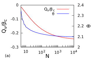
with , , , and the classical bound is found to be . Again the observables are taken as , The results are presented in Fig. 6. We see that (42) is violated by the ground state of the LMG Hamiltonian, and that the violation is not so large, but significant; this time it actually decreases slowly with .


At this point it is worth mentioning that the detection of nonlocality in this case can be realized by measuring the total spin components and their fluctuations: these quantities can be measured with a great precision in current experiments with cold atoms and ions, for instance using the spin polarization spectroscopy. Indeed, the considered Bell inequality requires measurements of , , , , and , where is a unit vector determining the spin direction in the second measurement.
It is worth mentioning that in the second paper [99], the more complex case of translational invariance was also considered – to this aim the parties were enumerated as if they were located in a 1D chain with periodic boundary conditions (a 1D ring). Recall that in this case the general form of a Bell inequality is
| (43) |
where are defined as before and ’s are translationally invariant two-body correlators given by
| (44) |
with for and for . The number of coefficients is now of order of 3, so the problem becomes intractable for large. We have, nevertheless found and classified all tight Bell inequalities for 3 and 4 parties, and provided some examples of five-party Bell inequalities that involve correlators between next neighbours only.
6 Conclusions
Let us conclude by listing several experimental setups in which nonlocality in many-body systems may be tested using the two-body Bell inequalities:
- •
Ultracold trapped atoms. Dicke states have been recently created in spinor Bose-Einstein condensates (BEC) of Rubidium atoms, via the parametric process of spin changing collisions, in which two atoms collide to produce a pair [111]. These recent experiments demonstrate the production of many thousands of neutral atoms entangled in their spin degrees of freedom. Dicke-like states can be produced in this way, with at least 28-particle genuine multi-party entanglement and a generalized squeezing parameter of dB. Similarly, Rubidium atoms of pseudo-spin 1/2 in BEC may be employed to generate scalable squeezed states (for the early theory proposal see [112], for experiments see[113]). Very recently non-squeezed (non-Gaussian) entangled states of many atoms [114] were generated in this way. The number of atoms used in these experiments are of order of thousands and larger. So far, these numbers and experimental errors and imperfections are too large, while the corresponding fidelities too small to detect many body non-locality. In principle, however, it is possible to perform these experiments with mesoscopic atom numbers (say ), controlling the atom number to a single atom level (see Ref. [115] for the resonant fluorescence detection of Rb87 atoms in a MOT, and Refs. [116, 117] for optically trapped spin 1/2 fermions).
- •
Ultracold trapped ions. Ultracold trapped ions with internal pseudo-spin ”talk” to each other via phonon excitations, and in some condition behave as spin chains with long range interaction. This was originally proposed in Ref. [118], using inhomogeneous magnetic fields, and in Ref. [119], employing appropriately designed laser-ion interactions. The pioneering experiments were reported in Refs. [120, 121]. While in the early theory studies [119, 122, 123, 124] spin interactions decaying with the third power of the distance were considered, it was experimentally demonstrated that management of phonon dispersion allows to achieve powers between 0.1 and 3 in the 2D arrays of traps [125]. Recent state of art represents the work on experimental realization of a quantum integer-spin chain with controllable interactions [126]. We have studied trapped ion systems in relation to long range spin chains and quantum chaos [127], and trapped-ion quantum simulation of tunable-range Heisenberg chains [128]. In the latter paper we demonstrated that significant violation of the Bell inequalities, discussed in this lecture, is possible even for the ground states of the models with large, but finite interaction range. The experimental scheme is presented in Fig. 7.

Figure 7: (a,b): Level scheme and setup for a possible implementation of spin-spin interactions in 171Yb+. (c,d): Interaction strengths between one ion in the center and the other ions, for (c) or (d) , and different detunings from the center-of-mass (COM) mode. We have used the parameters specified in (b). Interactions are compared with the interactions of the Haldane-Shastry (HS) model (brown lines), and with interactions (green lines). - •
Ultracold atoms in nanostructures. Yet another possibility concerns systems of ultracold atoms trapped in the vicinity of tapered fibers and optical crystals (band gap materials). The experimental progress in coupling of ultracold atomic gases to nanophotonic waveguides, initiated by Refs. [129, 130, 131], is very rapid (cf. [132]). Early theoretical studies concerned remarkable optical properties of these systems (cf. [133, 134, 135, 136]). Ideas and proposals concerning realization of long range spin models were developed more recently, and mainly in Refs. see [137, 138, 139].
- •
Cold and ultracold atomic ensembles. Last, but not least, one should consider cold and ultracold ensembles (for an excellent review see [140]), in which, by employing quantum Faraday effect, one can reach unprecendented degrees of squeezing of the total atomic spin (cf. [141, 142]), and unprecendented degrees of precision of quantum magnetometry (cf. [143]). Note that in many concrete realisations the many body Bell inequalities derived in this paper require precise measurements of the total spin components, and their quantum fluctuations. Quantum Faraday effect, or in other words spin polarization spectroscopy, seems to be a perfect method to achieve this goal; note that in principle it allows also to reach spatial resolution, and/or to measure spatial Fourier components of the total spin [144, 145].
Acknowledgements.
We thank Joe Eberly, Christian Gogolin, Markus Oberthaler, Julia Stasińska, and Tamás Vértesi for enlightening discussions. This work was supported by Spanish MINECO projects FOQUS, DIQIP CHIST-ERA, and AP2009-1174 FPU PhD grant. We acknowledge also EU IP SIQS, ERC AdG OSYRIS, ERC CoG QITBOX, and The John Templeton Foundation. R. A. acknowledges Spanish MINECO for the Juan de la Cierva scholarship.References
- [1] \BYEinstein A., Podolsky B., \atqueRosen N. \INPhys. Rev.47193577.
- [2] \BYBohm D. \TITLEQuantum Theory, (Prentice Hall, Englewood Cliffs, NJ) 1951.
- [3] \BYBell J.S. \INPhysics 11964195-200.
- [4] \BYBell J.S. \TITLESpeakable and Unspeakable in Quantum Mechanics: Collected Papers on Quantum Philosophy, edited by A. Aspect, (Cambridge University Press, Cambridge) 2004.
- [5] \BYBrunner N., Cavalcanti D., Pironio S., Scarani V., \atqueWehner S. \INRev. Mod. Phys.862014419 .
- [6] \BYBrunner N., Gühne O., \atqueHuber M. (Eds.) \TITLEFifty years of Bell’s theorem, special issue of \INJ. Phys. A: Math. Theor.472014no. 42.
- [7] \BYAugusiak R., Demianowicz M., \atqueAcín A. \INJ. Phys. A: Math. Theor.472014424002.
- [8] \BYClauser J. F., Horne M. A., Shimony A., \atqueHolt R. A. \INPhys. Rev. Lett. 231969880.
- [9] \BYEkert A.K. \INPhys. Rev. Lett.671991661.
- [10] \BYBarrett J., Hardy L., \atqueKent A. \INPhys. Rev. Lett.952005010503.
- [11] \BYAcín A. et al. \INPhys. Rev. Lett.982007230501.
- [12] \BYPironio S. et al. \INNature46420101021.
- [13] \BYColbeck R. \TITLEPhD thesis: Quantum And Relativistic Protocols For Secure Multi-Party Computation, (University of Cambridge, Cambridge) 2007.
- [14] \BYColbeck R. \atqueKent A. \INJ. Phys. A: Math. Theor.442011095305.
- [15] \BYWheeler J.A. \atqueŻurek W. H. (Eds.) \TITLEQuantum Theory and Measurement, (Princeton University Press, Princeton) 1984.
- [16] \BYQian X.-F. \atqueEberly J.H. \INOpt. Lett.3620114110.
- [17] \BYQian X.-F., Little B., Howell J.C., \atqueEberly J.H. arXiv:1406.3338.
- [18] \BYHeisenberg M. \INNature4592009164-165.
- [19] \BYSuarez A. \atqueAdams P. (Eds.) \TITLEIs Science Compatible with Free Will?: Exploring Free Will and Consciousness in the Light of Quantum Physics and Neuroscience, (Springer, Berlin) 2013.
- [20] \BYBabai L., Fortnow L., \atqueC. Lund \INComp. Complexity1 (1)19913.
- [21] \BYAvis D., Imai H., Ito T., \atqueSasaki Y quant-ph/0404014.
- [22] \BYWerner R.F. \INPhys. Rev. A4019894277.
- [23] \BYHorodecki R., Horodecki P., Horodecki M., \atqueHorodecki K. \INRev. Mod. Phys.812009865.
- [24] \BYGisin, N. \INPhys. Lett. A1541991201.
- [25] \BYPopescu S. \atqueRohrlich D. \INPhys. Lett. A1661992293.
- [26] \BYBarrett J. \INPhys. Rev. A652002042302.
- [27] \BYAugusiak R., Demianowicz M., Tura J., \atqueAcín A. arXiv:1407.3114.
- [28] \BYSachdev S. \TITLEQuantum Phase Transitions, (Cambridge University Press, Cambridge) 1999.
- [29] \BYAugusiak R., Cucchietti F. M., \atqueLewenstein M., in \TITLEModern theories of correlated electron systems, edited by \NAMECabra D.C., Honecker A., \atquePujol P. \INLecture Notes in Physics843 Springer-Verlag, Berlin 2002, pp. 245-295.
- [30] \BYLewenstein M., Sanpera A., and Ahufinger V. \TITLEUltracold atoms in Optical Lattices: simulating quantum many body physics, (Oxford University Press, Oxford) 2012.
- [31] \BYOsterloh A., Amico L., Falci G., \atqueFazio R. \INNature4162002608.
- [32] \BYOsborne T. J. \atqueNielsen M. A. \INPhys. Rev. A662002032110.
- [33] \BYVerstraete F., Popp M., \atqueCirac J. I. \INPhys. Rev. Lett.922004027901.
- [34] \BYVerstraete F., Martín-Delgado M. A., \atqueCirac J. I. \INPhys.Rev.Lett.922004087201.
- [35] \BYVidal G., Latorre J. I., Rico E., \atqueKitaev A. \INPhys. Rev. Lett.902003227902.
- [36] \BYCalabrese P., Cardy J. \atqueDoyon B. (Eds.) \TITLEEntanglement entropy in extended quantum systems, special issue of \INJ. Phys. A422009500301.
- [37] \BYEisert J., Cramer M., \atquePlenio M. B. \INRev. Mod. Phys.822010277.
- [38] \BYVerstraete F., Wolf M. M., Pérez-García D., \atqueCirac J. I. \INPhys. Rev. Lett.962006220601.
- [39] \BYLi H. \atqueHaldane F. D. M. \INPhys. Rev. Lett.1012008010504.
- [40] \BYKitaev A. \atquePreskill J. \INPhys. Rev. Lett.962006110404.
- [41] \BYLevin M. \atqueWen X.-G. \INPhys. Rev. Lett.962006110405.
- [42] \BYWerner R. F. \atqueWolf M. M. \INPhys. Rev. A642001032112.
- [43] \BYŻukowski M. \atqueBrukner Č. \INPhys. Rev. Lett.882001210401.
- [44] \BYŚliwa C. \INPhys. Lett. A3172003165; \BYŚliwa C. arXiv:quant-ph/0305190.
- [45] \BYBancal J.-D., Gisin N., \atquePironio S. \INJ. Phys. A: Math. Theor.432010385303.
- [46] \BYAolita L., Gallego R., Cabello A., \atqueAcín, A. \INPhys. Rev. Lett.1082012100401.
- [47] \BYBakr W. S., Gillen J. I., Peng A., Foelling S., \atqueGreiner M. \INNature462200974-77.
- [48] \BYSherson J. F., Weitenberg C., Endres M., Cheneau M., Bloch I., \atqueKuhr S. \INNature467201068.
- [49] \BYHorodecki P \INPhys. Lett. A2321997333.
- [50] \BYSanpera A., Tarrach R., \atqueVidal G. \INPhys. Rev. A581998826.
- [51] \BYSamsonowicz J., Kuś M., \atqueLewenstein M. \INPhys. Rev. A762007022314.
- [52] \BYŻukowski M., Zeilinger A., Horne M. A., \atqueEkert A. K. \INPhys. Rev. Lett.7119934287.
- [53] \BYGühne \atqueTóth G. \INPhys. Rep.47420091 .
- [54] \BYDoherty A. C., Parrilo P. A., \atqueSpedalieri F. M. \INPhys. Rev. Lett.882002187904.
- [55] \BYHulpke F. \atqueBruß D. \INJ. Phys. A: Math. Gen.3820055573.
- [56] \BYGurvits L. \INSTOC692003448.
- [57] \BYChoi M.-D. \INProc. Symp. Pure Math.381982583.
- [58] \BYPeres A. \INPhys. Rev. Lett.7719961413.
- [59] \BYHorodecki M., Horodecki P., \atqueHorodecki R. \INPhys. Lett. A19962231.
- [60] \BYHorodecki M., Horodecki P., \atqueHorodecki R. \INPhys. Rev. Lett.8019985239.
- [61] \BYBennett C. H., DiVincenzo D. P., Smolin J. A., \atqueWootters W. K. \INPhys. Rev. A5419963824.
- [62] \BYVedral V., Plenio M. B., Rippin M. A., \atqueKnight P. L. \INPhys. Rev. Lett.7819972275.
- [63] \BYDiVincenzo D. P., Fuchs C. A., Mabuchi H, Smolin J. A., Thapliyal, \atqueUhlmann A. in \TITLEProceedings of the first NASA International Conference on Quantum Computing and Quantum Communication (Springer-Verlag, Berlin) 1998.
- [64] \BYLaustsen T., Verstraete F., \atquevan Enk S. J. \INQuantum Inf. Comput.3200364.
- [65] \BYNielsen M. A. \INPhys. Rev. Lett.831999436.
- [66] \BYVidal G. \INJ. Mod. Opt.472000355.
- [67] \BYJonathan D. \atquePlenio M. B \INPhys. Rev. Lett.8319991455.
- [68] \BYHorodecki M., Sen(De) A., \atqueSen U. \INPhys. Rev. A702004052326.
- [69] \BYHorodecki M. \INQuant. Inf. Comput.120013.
- [70] \BYPlenio M. B. \atqueVirmani S. \INQuant. Inf. Comp.720071.
- [71] \BYLubkin E. \INJ. Math. Phys.1919781028.
- [72] \BYLloyd, S. \atquePagels H. \INAnn. Phys.1881988186.
- [73] \BYPage D. N. \INPhys. Rev. Lett.7119931291.
- [74] \BYBengtsson I. \atqueŻyczkowski K. \TITLEGeometry of Quantum States, (Cambridge University Press, Cambridge) 2006.
- [75] \BYFoong S. K. \atqueKanno S. \INPhys. Rev. Lett.7219941148.
- [76] \BYSen S. \INPhys. Rev. Lett.7719961.
- [77] \BYSanchez-Ruíz J. \INPhys. Rev. E5219955653.
- [78] \BYHastings M. B. \INJ. Stat. Mech.: Theory and Exp.2007P08024.
- [79] \BYLieb E. H. \atqueRobinson D. W. \INComm. Math. Phys.281972251.
- [80] \BYMasanes L. \INPhys. Rev. A802009052104.
- [81] Dür W., Hartmann L., Hein M., Lewenstein M., \atqueBriegel H.-J \INPhys. Rev. Lett.942005097203.
- [82] \BYEisert J. \atqueOsborne T. \INPhys. Rev. Lett.972006150404.
- [83] \BYLatorre J.-I. \atqueRiera A. \INJ. Phys. A422009504002.
- [84] \BYCalabrese P. \atqueCardy J. \INJ. Phys. A422009504005.
- [85] \BYBrandão F. G. S. L. \atqueHorodecki M. \INNat. Phys.92013721-726.
- [86] \BYWolf M. M. \INPhys. Rev. Lett.962006010404.
- [87] \BYGioev D. \atqueKlich I. \INPhys. Rev. Lett.962006100503.
- [88] \BYFarkas S. \atqueZimboras Z. \INJ. Math. Phys.482007102110.
- [89] \BYŻyczkowski P., Horodecki P., Sanpera A., \atqueLewenstein M. \INPhys. Rev. A581998883.
- [90] \BYVidal G. \atqueWerner R. F. \INPhys. Rev. A652002032314.
- [91] \BYGroisman B., Popescu S., \atqueWinter A. \INPhys. Rev. A722005032317.
- [92] \BYWolf M. M., Verstraete F., Hastings M. B., \atqueCirac J. I. \INPhys. Rev. Lett.1002008070502.
- [93] \BYVerstraete F., Popp M., \atqueCirac J. I. \INPhys. Rev. Lett.922004027901.
- [94] \BYVidal G. \INPhys. Rev. Lett.912003147902.
- [95] \BYPerez-García D., Verstraete F., Wolf M. M., \atqueCirac J. I. \INQuant. Inf. Comput.72007401.
- [96] \BYVerstraete \atqueCirac J. I., cond-mat/0407066.
- [97] \BYSchuch N., Wolf M. M., Verstraete F., \atqueCirac J. I. \INPhys. Rev. Lett.982007140506.
- [98] \BYTura J, Augusiak R., Sainz A .B., Vértesi T., Lewenstein M., Acín A. \INScience34420141256-1258.
- [99] \BYTura J., Sainz A. B., Vértesi T., Lewenstein M., Acín A., \atqueAugusiak R. \INJ. Phys. A472014424024, in special issue \TITLE50 years of Bell’s Theorem.
- [100] \BYTóth G. \INPhys. Rev. A712005010301.
- [101] \BYKorbicz J., Cirac J. I., Wehr J., \atqueLewenstein M. \INPhys. Rev. Lett.942005153601.
- [102] \BYTóth G., Knapp C., Gühne O., \atqueBriegel H. J. \INPhys. Rev. Lett.992007250405.
- [103] \BYCramer M., Plenio M. B., \atqueWunderlich H. \INPhys. Rev. Lett.1062011 020401.
- [104] \BYMarkiewicz M., Laskowski W., Paterek T., \atqueŻukowski M. \INPhys. Rev. A872013034301.
- [105] \BYBrunner N., Sharam J., \atqueVértesi T. \INPhys. Rev. Lett.1082012110501.
- [106] \BYWieśniak M., Nawareg M., \atqueŻukowski M. \INPhys. Rev. A862012042339.
- [107] \BYWürflinger L. E., Bancal J.-D., Acín A., Gisin N., \atqueVértesi T. \INPhys. Rev. A862012032117.
- [108] \BYGittsovich O., Hyllus P., \atqueGühne O. \INPhys. Rev. A822010032306.
- [109] \BYLipkin H. J., Meshkov N., \atqueGlick A. J. \INNucl. Phys.621965188-198.
- [110] \BYDicke R. H. \INPhys. Rev.93195499-110.
- [111] \BYLücke B., Peise J., Vitagliano G., Arlt J., Santos L., Tóth G., \atqueKlempt C. \INPhys. Rev. Lett.1122014155304.
- [112] \BYSørensen A. S., Duan L.-M., Cirac J. I., \atqueZoller P. \INNature409200163.
- [113] \BYMuessel W., Strobel H., Linnemann D, Hume D.B., \atqueOberthaler M.K., arXiv:1405.6022.
- [114] \BYStrobel H., Muessel W., Linnemann D., Zibold T., Hume D.B., Pezzè L., Smerzi A., \atqueOberthaler M.K. \INScience3452014424.
- [115] \BYHume D.B., Stroescu I., Joos M., Muessel W., Strobel H., \atqueOberthaler M.K. \INPhys. Rev. Lett.1112013253001.
- [116] \BYWenz A.N., Zürn G., Murmann S., Brouzos I., Lompe T., \atqueJochim S. \INScience3422013457-460.
- [117] \BYZürn G., Wenz A.N., Murmann S., Bergschneider A., Lompe T., \atqueJochim S. \INPhys. Rev. Lett.1112013175302.
- [118] \BYMintert F. \atqueWunderlich C. \INPhys. Rev. Lett.872001257904.
- [119] \BYPorras D. \atqueCirac J.I. \INPhys. Rev. Lett.922004207901.
- [120] \BYFriedenauer A., Schmitz H., Glueckert J.T., Porras D., \atqueSchätz T. \INNature Phys.42008757.
- [121] \BYKim K., Chang M.-S., Korenblit S., Islam R., Edwards E.E., Freericks J.K., Lin G.-D, Duan L.-M., \atqueMonroe C. \INNature4652010590.
- [122] \BYX.-L. Deng, D. Porras, and J. I. Cirac, Phys. Rev. A 72, 063407 (2005).
- [123] \BYHauke P., Cucchietti F.M., Müller-Hermes A., Bauls M.-C., Cirac J.I., \atqueLewenstein M. \INNew J. Phys.122010113037.
- [124] \BYMaik M., Hauke P., Dutta O., Zakrzewski J., \atqueLewenstein M. \INNew J. Phys.142012113006.
- [125] \BYBritton J.W., Sawyer B.C., Keith A.C., Wang C.-C. J., Freericks J.K., Uys H., Biercuk M.J., \atqueBollinger J.J. \INNature4842012489.
- [126] \BYSenko C., Richerme P., Smith J., Lee A., Cohen I., Retzker A., \atqueMonroe C., arXiv:1410.0937.
- [127] \BYGraßT., Julia-Díaz B., Kuś M., \atqueLewenstein M. \INPhys. Rev. Lett.1112013090404.
- [128] \BYGraßT. \atqueLewenstein M. \INEPJ Quantum Technology1:82014.
- [129] \BYNayak K.P., Melentiev P.N., Morinaga M., Kien F.L., Balykin V.I., \atqueHakuta K. \INOpt. Express1520075431.
- [130] \BYVetsch E., Reitz D., Sagu G., Schmidt R., Dawkins S.T., \atqueRauschenbeutel A. \INPhys. Rev. Lett.1042010203603.
- [131] \BYGoban A., Choi K.S., Alton D.J., Ding D., Lacrote C., Pototschnig M., Thiele T., Stern N.P., \atqueKimble H.J. \INPhys. Rev. Lett.1092012033603.
- [132] \BYGoban A., Hung C.-L., Yu S.-P, Hood J.D., Muniz J.A., Lee J.H., Martin M.J., McClung A.C., Choi K.S., Chang D.E., Painter O., \atqueKimble H.J. arXiv:1312.3446.
- [133] \BYKien F.L. and Hakuta K. \INPhys. Rev. A772008013801.
- [134] \BYZoubi H. \atqueRitsch H. \INNew J. Phys.122010103014.
- [135] \BYChang Y., Gong Z.R., \atqueSun C.P. \INPhys. Rev. A832011013825.
- [136] \BYChang D.E., Jiang L., Gorshkov A.V., \atqueKimble H.J. \INNew J. Phys.142012063003.
- [137] \BYChang D.E., Cirac J.I., \atqueKimble H.J. \INPhys. Rev. Lett.1102013113606.
- [138] \BYGonzález-Tudela A., Hung C.-L., Chang D.E., Cirac J.I., \atqueKimble H.J., arXiv:1407.7336.
- [139] \BYDouglas J.S., Habibian H., Gorshkov A.V., Kimble H.J., \atqueChang D.E, arXiv:1312.2435.
- [140] \BYHammerer K., Sørensen A.S., \atquePolzik E.S. \INRev. Mod. Phys.8220101041.
- [141] \BYNapolitano M., Koschorreck M., Dubost B., Behbood N., Sewell R.J., \atqueMitchel M.W.l \INNature4712011486-489.
- [142] \BYSewell R.J., Napolitano M., Behbood N., Colangelo G., Martin Ciurana F., \atqueMitchel M.W.l \INPhys. Rev. X42014021045.
- [143] \BYLucivero V.G., Anielski P., Gawlik W., \atqueMitchel M.W. \INRev. Sci. Instrum.852014113108.
- [144] \BYEckert K., Romero-Isart O., Rodriguez M., Lewenstein M., Polzik E.S., \atqueSanpera A. \INNature Phys.4200850.
- [145] \BYRogers B, Paternostro M., Sherson J.F., \atqueDe Chiara G. \INPhys. Rev. A902014043618.
- [146] \BYGe Y. and Eisert J. arXiv:1411.2995.