A Second Order TV-type Approach for Inpainting and Denoising Higher Dimensional Combined Cyclic and Vector Space Data

Ronny Bergmann ^†^†thanks: Departement of Mathematics, Technische Universität Kaiserslautern, Paul-Ehrlich-Str. 31, 67663 Kaiserslautern, Germany
bergmann@mathematik.uni-kl.de. Andreas Weinmann ^†^†thanks: Department of Mathematics, Technische Universität München and Fast Algorithms for Biomedical Imaging Group, Helmholtz-Zentrum München, Ingolstädter Landstr. 1, 85764 Neuherberg, Germany
andreas.weinmann@tum.de

August 24, 2026

Abstract

Abstract. In this paper we consider denoising and inpainting problems for higher dimensional combined cyclic and linear space valued data. These kind of data appear when dealing with nonlinear color spaces such as HSV, and they can be obtained by changing the space domain of, e.g., an optical flow field to polar coordinates. For such nonlinear data spaces, we develop algorithms for the solution of the corresponding second order total variation (TV) type problems for denoising, inpainting as well as the combination of both. We provide a convergence analysis and we apply the algorithms to concrete problems.

Keywords.

Higher order total variation minimization, vector-valued TV, cyclic data, combined denoising and inpainting, cyclic proximal point algorithm.

1 Introduction

One of the most well known methods for edge-preserving image denoising is the variational approach minimizing the Rudin-Osher-Fatemi (ROF) functional [70]. In its basic form, it deals with scalar data. Related variational approaches for vector space valued data have gained a lot of interest in the literature and are still topic of ongoing research; we exemplarily refer to [12, 67, 42, 61] and the references therein. In this paper, we consider TV-type functionals incorporating first and second order differences for the nonlinear data spaces which combine vector space valued data —in the following called linear space data to avoid confusion— and vectors of cyclic data. In these spaces, we deal with denoising and inpainting problems as well as simultaneous inpainting and denoising problems.

Image inpainting is a problem arising in many applications in image processing, image analysis and related fields. Examples are restoring scratches in photographs, removal of superimposed objects, dealing with an area removed by a user, digital zooming as well as edge decoding. Principally, any missing data situation —whatever the reason might be— results in an inpainting problem. This is not restricted to 2D images. Further examples are defects in audio and video recordings, or in seismic data processing. In this respect, also interpolation, approximation, and extrapolation problems may be viewed as inpainting problems. We recommend the survey [45] and Chapter 6 of [27] as well as [16, 18] for an overview on inpainting and for further applications. There are various conceptionally different approaches to inpainting, cf. [27, 45] and [18] which also includes some comparison. Among these are methods based on linear transforms from harmonic analysis such as curvelets and shearlets which are combined with a sparsity approach based on $\ell^{1}$ minimization on the corresponding coefficients [17, 33, 32, 51]. Other approaches are based on (often nonlinear) PDE and variational models, cf., e.g., [13, 19, 25, 26, 34, 57, 58, 59, 60, 74, 78].
In general, exemplar-based and sparsity-based methods perform better for filling large texture areas, whereas diffusion-based and variational techniques yield better results for natural images. Among the variational techniques applied, total variation (TV) minimization is one of the prominent models. The minimizer of the corresponding TV functional yields the inpainted image. TV inpainting works well for elongated inpainting areas but has problems with larger gap connections. In such situations higher order, in particular curvature based, schemes perform better.

The first TV regularized model was proposed in [70] for denoising. It was first applied to missing data situations/inpainting in [4, 24]. Further references for TV based image inpainting are [15, 28, 74]. In contrast to classical methods, the results are typically not over-smoothed; however, it is well known that these minimizers very often show ‘staircasing’ effects, i.e. the result is often piecewise constant, although the underlying signal varies smoothly in the corresponding regions. In order to avoid staircasing, higher order and, in particular, second order differences and derivatives (in a continuous domain setting), are often employed. References are the pioneering work [20] as well as [14, 21, 23, 30, 31, 48, 53, 55, 56, 71, 72, 73]. TV functionals for linear space valued data were considered in [12] in the context of linear color spaces. The papers [63, 64] deal with denoising and inpainting in the RGB color space using linear combinations of first and second order terms. A total generalized variational model can be found, e.g., in [61]. In contrast to applying pure second order terms or linear combinations of first and second order terms, total generalized variational approaches try to find some optimal balancing between the first and second derivatives. The advantage is that the related schemes better preserve the edge structures. A detailed description may be found in [14]. The authors of [61] obtain a model for denoising linear space valued color data. Second order total generalized variation was generalized for tensor fields in [80].

However, in many applications, data having values in nonlinear spaces appear. Examples are diffusion tensor images [5, 65], color images based on non-flat color models [22, 50, 52, 81] or motion group-valued data [69, 79]. Due to its importance, processing such manifold valued data has gained a lot of interest in recent years. To mention only some examples, wavelet-type multi scale transforms for manifold data have been considered in [44, 79, 83]. Statistical issues on Riemannian manifolds are the topic of [10, 11, 37, 62, 66] and circular data are, in particular, considered in [36, 49]. Furthermore, manifold-valued partial differential equations are studied in [29, 43, 77].

For TV functionals for manifold-valued data, an analysis from a theoretical viewpoint has been carried out in [40, 39]. These papers extend previous work [38] on $\mathbb{S}^{1}$ -valued functions where, in particular, the existence of minimizers of certain TV-type energies is shown. An algorithm for TV minimization on Riemannian manifolds was proposed in [54]. This approach uses a reformulation as a multi label optimization problem with an infinite number of labels and a subsequent convex relaxation. An approach for linear spaces using a relaxation of the label optimization problem as well was presented in [41]. First order TV minimization for $\mathbb{S}^{1}$ -valued data has been considered in [76, 75]. In particular, these authors consider inpainting for $\mathbb{S}^{1}$ -valued data in a first order TV setup. We proposed a different approach to first order TV minimization for manifold-valued data via cyclic and parallel proximal point algorithms in [85]. We established a second order setup for denoising $\mathbb{S}^{1}$ -valued data based on cyclic proximal point algorithms in [6]. Inpainting for $\mathbb{S}^{1}$ -valued data was considered in the authors’ conference proceeding [7].

Data consisting of combined cyclic and linear space components appear in various contexts. For example, such data appear when dealing with nonlinear color spaces such as HSV, HSL, HSI or HCL. Such data also appear in the context of optical flows. When considering the flow vectors between consecutive images in polar coordinates which means separating magnitude and direction, the resulting data takes its values in $\mathbb{R}\times\mathbb{S}^{1}$ . In this context, this approach is natural and interesting and seems promising to improve the results obtained with the usual $\mathbb{R}^{2}$ -valued approach. In principle, whenever data is given as vectors of polar coordinates, we are in the combined cyclic and real-valued setup of data in $(\mathbb{S}^{1})^{m}\times\mathbb{R}^{m}$ considered in this paper.

Contributions.

In this paper, we consider inpainting, denoising as well as combined inpainting and denoising problems for combined cyclic and linear space valued images in $(\mathbb{S}^{1})^{m}\times\mathbb{R}^{n}$ based on a second order TV-type formulation. We consider two variational models: the first model deals with the noise free situation whereas the second one also considers the noisy case combining denoising and inpainting (including pure denoising by specifying the inpainting area as the empty set). In our nonlinear setting, these higher order approaches avoid unwanted staircasing effects as well. For combined cyclic and linear space data, we derive solvers for these variational problems based on cyclic proximal point algorithms. We provide a convergence analysis for both the noisy and the noise free model based algorithms developed in this paper. For both algorithms, we show the convergence to a minimizer under certain restrictions which are typical when dealing with nonlinear data. In particular, we assume the data to be dense enough meaning that they are locally (and not necessarily globally) nearby. We apply our algorithms to denoising, inpainting and combined denoising and inpainting in the nonlinear HSV color space. Furthermore, we apply our algorithms for denoising frames in volumetric phase-valued data – in our case, frames of a 2D film. Our approach is based on utilizing the neighboring $k$ frames to incorporate the temporal neighborhood. The idea generalizes to arbitrary data spaces and volumes consisting of layers of 2D data.

The novelties of the present work in relation to the authors previous work [6, 7] are as follows. (i) In contrast to [6, 7] we consider the more general, practically relevant, data spaces $(\mathbb{S}^{1})^{m}\times\mathbb{R}^{n}$ here. In contrast to general manifolds, these product spaces still bear enough structure relevant for our purposes. We point out that both, the algorithmic and analysis part, are more involved than only component-wise considering the $\mathbb{S}^{1}$ -valued or real-valued situation. (ii) Concerning the algorithmic part, we compute proximal mappings of constrained problems arising in inpainting situations in this work. This is even new for $\mathbb{S}^{1}$ data. In [7], we used a less natural projection approach generalizing [6]. (iii) Concerning the analysis, we here include an inpainting setup. The conference proceeding [7] does not contain an analysis and [6] considers functionals for denoising $\mathbb{S}^{1}$ valued data. A more detailed discussion may be found at the end of the paper.

Outline of the paper.

In Section 2 we introduce the variational models we consider for inpainting and denoising of combined cyclic and linear space data in this paper. We start with vector space data in Subsection 2.1; then we define absolute differences for combined cyclic and vector space data in Subsection 2.2 which allow us to derive the corresponding variational models for combined cyclic and vector space data. This is done in Subsection 2.3 for both inpainting noise free combined cyclic and vector space data as well as inpainting and denoising combined cyclic and vector space data. In Section 3 we develop algorithms for minimizing the variational models introduced previously. These algorithms base on the cyclic proximal point algorithm we present in Subsection 3.1. We present explicit formulas for the proximal mappings needed for inpainting in Subsection 3.2. Using these explicit representations, we derive a cyclic proximal point algorithm for inpainting both the noisy and noise free combined cyclic and vector space data in Subsection 3.3. The convergence analysis of both algorithms is the topic of Section 3.4. Finally, in Section 4 we apply the derived algorithms to various concrete situations. We consider denoising data living in the nonlinear HSV color space in Subsection 4.1. Then we consider inpainting for noise-free as well as noisy data in such color spaces in Subsection 4.2. Finally, we apply our algorithms for denoising frames of a $\mathbb{S}^{1}$ -valued 2D film in Subsection 4.3.

2 Second order variational models for inpainting and denoising combined cyclic and linear space data

In this section we derive models for denoising, inpainting as well as simultaneous inpainting and denoising data having cyclic and linear space components. In Subsection 2.1, we first concentrate on introducing the considered models based on first and second order absolute finite differences restricting to the linear space setting. In Subsection 2.2 we obtain suitable definitions for absolute differences for combined cyclic and vector space data. In Subsection 2.3, we use these definitions to obtain inpainting and simultaneous inpainting and denoising models for combined cyclic and linear data. In particular, denoising is covered by considering the empty set as inpainting region.

Let us fix some notations. We denote by $(f_{i,j})_{(i,j)\in\Omega}$ , $\Omega_{0}\coloneqq\{1,\ldots,N\}\times\{1,\ldots,M\}$ images of size $N$ by $M$ , which can also be seen as functions $f(i,j)$ on the image domain $\Omega_{0}$ . For any subset $\Omega\subset\Omega_{0}$ of pixel indices $\Omega^{C}\coloneqq\Omega_{0}\backslash\Omega$ denotes the complement of $\Omega$ in $\Omega_{0}$ . Each entry $f_{i,j}\in\mathcal{X}$ is called a pixel value, where $\mathcal{X}$ is some data space. Our main focus is the $(m+n)$ -dimensional space $\mathcal{X}\coloneqq(\mathbb{S}^{1})^{m}\times\mathbb{R}^{n}$ . On a data space $d_{\mathcal{X}}(x,y),D_{1}(x,y),D_{2}(x,y,z)$ , and $D_{1,1}(w,x,y,z)$ denote the distance on $\mathcal{X}$ , the absolute first, absolute second, and absolute second order mixed differences. If the space is clear from the context or the setting holds for all spaces, we omit the $\mathcal{X}$ . The elements $x=(x_{1},\ldots,x_{n})^{\mathrm{T}}\in\mathbb{R}^{n}$ are column vectors, where $\cdot^{\mathrm{T}}$ denotes the transposition. For two vectors $x,y\in\mathbb{R}^{n}$ we denote by $\langle x,y\rangle\coloneqq x^{\mathrm{T}}y$ the inner product. By $(x)_{2\pi}\in[-\pi,\pi)$ we denote the elementwise modulo operation, i.e. the unique value such that $x=2\pi k+(x)_{2\pi}$ , $k\in\mathbb{Z}^{n}$ . Finally, for matrices $x=(x_{i,j})_{i=1,j=1}^{n,d}\in\mathbb{R}^{n\times d}$ we denote the columns by $x^{(j)}$ .

2.1 Inpainting and denoising vector space data

The Rudin-Osher-Fatemi (ROF) functional [70]

\sum_{i,j}(f_{i,j}-x_{i,j})^{2}+\alpha\sum_{i,j}\lVert\nabla x_{i,j}\rVert,\quad\alpha>0,

is one of the most well known and most popular functionals in variational image processing. In its penalized form, it consists of two terms: the first term measures the distance to the data $f$ the second term is a TV regularizer where $\nabla$ denotes the discrete gradient operator, usually implemented as first order forward differences in vertical and horizontal directions. Both an isotropic version using the euclidean length or $2$ -norm and an anisotropic version employing the sum of absolute values or $1$ -norm for the second term are widely used. In this work we will restrict ourselves to the anisotropic version. In this form, the ROF Model is typically used for denoising purposes. To avoid the appearing staircasing effect, often higher order and, in particular, second order differences (respectively, derivatives, in a continuous domain setting) are employed [20, 14, 21, 23, 30, 31, 48, 53, 55, 56, 71, 72, 73].

Denoising.

For pure denoising we consider the discrete second order TV-type functional

\begin{split}J(x)&=F(x;f)+\alpha\operatorname{TV}_{1}(x)\\ &\qquad+\beta\operatorname{TV}_{2}(x)+\gamma\operatorname{TV}_{1,1}(x),\end{split}

(1)

where $x,f$ are images defined on the image domain $\Omega_{0}$ denotes the image domain. The data values $f_{i,j}$ itself live in a certain data space. Then the data term $F(x;f)$ for given data $f$ reads

\displaystyle F(x;f)

\displaystyle=\frac{1}{2}\sum_{i,j=1}^{N,M}d(f_{i,j},x_{i,j})^{2},

(2)

where $d$ is a distance on the data space. For data living in a vector space, $d(f_{i,j},x_{i,j})=\lVert f_{i,j}-x_{i,j}\rVert$ is an appropriate choice. In the pure linear space data situation, the above quadratic data term (2) corresponds to a Gaussian noise model. For other types of noise, different data terms are more appropriate; e.g., for Laplacian noise the term $F(x;f)=\sum_{i,j=1}^{N,M}d(f_{i,j},x_{i,j})$ is appropriate; cf. also [63].

The first order difference component $\alpha\operatorname{TV}_{1}(x)$ is given by

\begin{split}\alpha\operatorname{TV}_{1}(x)&=\alpha_{1}\sum_{i,j=1}^{N-1,M}D_{1}(x_{i,j},x_{i+1,j})\\ &\qquad+\alpha_{2}\sum_{i,j=1}^{N,M-1}D_{1}(x_{i,j},x_{i,j+1})\\ &\qquad+\frac{\alpha_{3}}{\sqrt{2}}\sum_{i,j=1}^{N-1,M-1}D_{1}(x_{i,j},x_{i+1,j+1})\\ &\qquad+\frac{\alpha_{4}}{\sqrt{2}}\sum_{i,j=1}^{N-1,M-1}D_{1}(x_{i,j+1},x_{i+1,j}).\end{split}

(3)

Again, for a vector space any norm of the ordinary absolute first order difference $D_{1}(x_{i,j},x_{i+1,j})=\lVert x_{i,j}-x_{i+1,j}\rVert$ is an appropriate choice. The first order TV term incorporates horizontal, vertical and both diagonal differences. The diagonals are incorporated to reduce unwanted anisotropy effects and are scaled by $\frac{1}{\sqrt{2}}$ to take the length of the diagonal on the pixel grid, i.e. the distance of two pixels, into account. We note that $J^{\prime}(x)=F(x;f)+(\alpha_{1},\alpha_{2},0,0)\operatorname{TV}_{1}(x)$ is just the vector version of the anisotropic discrete ROF functional above. Using the notation

	$\displaystyle D_{2}(x,y,z)$	$\displaystyle=\lVert x-2y+z\rVert$	(4)
and
	$\displaystyle D_{1,1}(x,y,u,v)$	$\displaystyle=\lVert x-y-u+v\rVert,$

for a norm of the standard second order differences for vector space data, the second order difference component, consisting of a horizontal and vertical component $\beta\operatorname{TV}_{2}(x)$ as well as a diagonal component $\gamma\operatorname{TV}_{1,1}(x),$ is given by

		$\displaystyle\begin{aligned} \mathllap{\beta\operatorname{TV}_{2}(x)}&=\beta_{1}\!\sum_{i=2,j=1}^{N-1,M}\!\!D_{2}(x_{i-1,j},x_{i,j},x_{i+1,j})\\ &\qquad+\beta_{2}\!\sum_{i=1,j=2}^{N,M-1}\!\!D_{2}(x_{i,j-1},x_{i,j},x_{i,j+1}),\end{aligned}$		(5)
		$\displaystyle\begin{aligned} \mathllap{\gamma\operatorname{TV}_{1,1}(x)}&=\gamma\!\!\!\!\sum_{i,j=1}^{N-1,M-1}\!\!\!\!D_{1,1}(x_{i,j},x_{i+1,j},x_{i,j+1},x_{i+1,j+1}).\end{aligned}$		(6)

We note that similar to the diagonal differences in the $\operatorname{TV}_{1}$ part the diagonal component $\gamma\operatorname{TV}_{1,1}(x)$ , which is based on the mixed second order difference $D_{1,1}$ , reduces unwanted anisotropy effects for the second order part. Actually, $D_{1,1}(x_{i,j},x_{i+1,j},x_{i,j+1},x_{i+1,j+1})$ may be interpreted as a diagonal difference: averaging $x_{i,j+1}$ and $x_{i+1,j}$ yields an estimate for the non-grid value $m=``x_{i+1/2,j+1/2}$ ”. Then $D_{2}(x_{i,j},m,x_{i+1,j+1})=D_{1,1}(x_{i,j},\\ x_{i+1,j},x_{i,j+1},x_{i+1,j+1})$ plays the role of a second order diagonal difference. Interchanging the roles of $x_{i,j+1},\\ x_{i+1,j}$ and $x_{i,j},x_{i+1,j+1}$ yields the other diagonal. Hence, diagonal differences are already incorporated in the second order term and we do not have to consider terms of the form $D_{2}(x_{i-1,j-1},x_{i+1,j+1},x_{i,j})$ for the reduction of anisotropy effects. The model parameters $\alpha_{1},\alpha_{2},\alpha_{3},\alpha_{4},\\ \beta_{1},\beta_{2},\gamma$ regulate the influence of the different TV terms.

One main reason for considering this anisotropic model is that it is computationally feasible for the nonlinear space of combined cyclic and vector space data considered in this paper as we will see later on. To our knowledge there are no previous algorithms dealing with any kind of second order TV-like problems in this nonlinear situation —neither in the isotropic nor in the anisotropic setup. As explained, we employ diagonal terms to milden unwanted effects caused by the anisotropic formulation.

Next, we consider suitable modifications of the above functional to obtain models for the inpainting problem with noisy and noiseless data. We start by first formulating the inpainting problem.

Inpainting problem in the presence of noise.

Given an image domain $\Omega_{0}=\{1,\ldots,N\}\times\{1,\ldots,M\},$ an inpainting region $\Omega\subset\Omega_{0}$ is a subset of the image domain $\Omega_{0}$ , where the pixel values $f_{i,j}$ , $(i,j)\in\Omega$ , are lost. The noiseless or noisy inpainting problems now consist of finding a function $x$ defined on $\Omega_{0}$ from data $f$ given on the complement $\Omega^{C}$ of the inpainting region, such that $x$ is a suitable extension to $f$ onto $\Omega$ and for the second case additionally denoised.

Inpainting without presence of noise.

To deal with the noiseless situation, we consider the following modification of the functional $J$ given by (1). Since the data is assumed to be noiseless, we add the constraint that the target variable agrees with the data on the complement of the inpainting region. Furthermore, the data term considers only those indices for which actually data are available. This eliminates the data term from the functional. More precisely, the second order variational inpainting problem considered in this paper reads for a vector space as

\begin{split}\argmin_{x}&\ \alpha\operatorname{TV}_{1}(x)+\beta\operatorname{TV}_{2}(x)+\gamma\operatorname{TV}_{1,1}(x),\\ &\text{ subject to }x_{i,j}=f_{i,j}\text{ for all }(i,j)\in\Omega^{C}.\end{split}

(7)

The TV terms $\operatorname{TV}_{1},$ $\operatorname{TV}_{2},$ $\operatorname{TV}_{1,1}$ are defined by (3), (5) and (6) using the difference terms $D_{1},D_{2},D_{1,1}$ based on a norm in the vector space. Due to the constraint they actually only act on those difference terms that affect an entry in the inpainting region.

Second order TV formulation of the inpainting problem for noisy data.

For the inpainting problem in presence of noise the requirement of equality on $\Omega^{C}$ is replaced by $x$ being a suitable, i.e., smooth approximation. In this case, we search for a minimizer of the following second order TV functional for cyclic data for inpainting:

\begin{split}J_{\Omega}(x)&=F_{\Omega^{C}}(x;f)+\alpha\operatorname{TV}_{1}(x)\\ &\qquad+\beta\operatorname{TV}_{2}(x)+\gamma\operatorname{TV}_{1,1}(x),\end{split}

(8)

where for any subset $B\subset\Omega_{0}$ of the image domain, we define

F_{B}(x;f)\coloneqq\frac{1}{2}\sum\nolimits_{(i,j)\in B}d(x_{i,j},f_{i,j})^{2}.

(9)

This means we use a data term that enforces similarity to the given data $f$ on $\Omega^{C}$ while applying a regularization based on (3),(5), and (6) for the whole image domain. Specifying the inpainting area as the empty set, we obtain the pure denoising problem (1).

2.2 Absolute differences for combined cyclic and vector space data

In order to implement the above variational inpainting problem (7) and the simultaneous inpainting and denoising problem (8) for combined cyclic and vector space data, we have to find suitable difference operators $D_{1},D_{2},D_{1,1}$ for data consisting of combined cyclic and linear space components. In order to do so, we first find suitable definitions for vectors of cyclic data. Then, we combine these definitions with those for the linear space case in a way suitable to the space of interest in this paper. We use the symbols $D_{\bullet}$ already introduced in (3) for the linear space case, also for the case of vectors of cyclic and combined data. We further unify the notation to $D(\cdot\,;\,w)$ for different weights $w$ . This overload is employed to avoid additional notation and should not cause confusion since the space under consideration will be clear from the context.

Let $w=(w_{j})_{j=1}^{d}\in\mathbb{R}^{d}$ , $w\neq 0$ , be a vector with $\sum_{j=1}^{d}w_{j}=0,$ and call such a vector $w$ a weight. Special cases are the binomial coefficients with alternating signs

\textstyle b_{d}=\left((-1)^{j+d-1}{d\choose{j-1}}\right)_{j=1}^{d+1}.

For the vectors $x^{(j)}\in\mathbb{R}^{n}$ , $j=1,\ldots,d$ , we employ the matrix $x\coloneqq\bigl(x^{(1)},\ldots,x^{(d)}\bigl)\in\mathbb{R}^{n\times d}$ to define the absolute finite difference $D$ for these vectors with respect to the weight $w\in\mathbb{R}^{d}$ by

D(x;w)=\lVert xw\rVert=\Big\lVert\sum_{j=1}^{d}w_{j}x^{(j)}\Big\rVert.

For $w=b_{d}$ , we obtain the forward differences of order $d$ for the vectors $x^{(1)},\ldots,x^{(d+1)}$ , i.e.

D_{d}(x)\coloneqq D(x;b_{d})=\Bigl\lVert\sum_{j=1}^{d+1}(-1)^{j+d-1}{\textstyle{d\choose{j-1}}}x^{(j)}\Bigl\rVert.

Another useful weight used in this paper is $w=b_{1,1}\coloneqq(-1,1,1,-1)$ . We denote the corresponding finite absolute difference by $D_{1,1}(x)\coloneqq D(x;b_{1,1})$ .

Example 2.1.

For three points $x_{1},x_{2},x_{3}\in\mathbb{R}^{n}$ and $w=b_{2}=(1,-2,1)^{\mathrm{T}}$ the second order absolute difference is given by $D_{2}(x_{1},x_{2},x_{3})=\lVert x_{1}-2x_{2}+x_{3}\rVert$ , cf. (4). This can be interpreted as measuring the distance from $y$ to the midpoint $m_{x}\coloneqq\frac{1}{2}(x_{1}+x_{3})$ of the line segment connecting $x_{1}$ and $x_{3}$ ; more precisely, we have $D_{2}(x_{1},x_{2},x_{3})=2\lVert\tfrac{1}{2}(x_{1}+x_{3})-x_{2}\rVert$ . The situation is shown in Figure 1 for $n=2$ , but also illustrates the situation for general $n>2$ in the plane defined by $x_{1},x_{2},x_{3}$ . For $n=1$ the situation simplifies to $x_{2}$ always lying on the line —though not necessarily the segment— connecting $x_{1}$ and $x_{3}$ .

Figure 1: The three points

x_{1},x_{2},x_{3}\in\mathbb{R}^{2}

illustrate the multivariate finite difference

D_{2}(x_{1},x_{2},x_{3})=2\lVert m_{x}-x_{2}\rVert

, i.e. the distance of

x_{2}

to the midpoint

m_{x}\coloneqq\tfrac{1}{2}(x_{1}+x_{3})

x_{1}

and

x_{3}

. This measures how “near” they are to lying equally distributed on a line segment in the right order.

We consider the cyclic case next. Let $\mathbb{S}^{1}$ denote the unit circle $\mathbb{S}^{1}\coloneqq\{p_{1}^{2}+p_{2}^{2}=1:p=(p_{1},p_{2})^{\mathrm{T}}\in\mathbb{R}^{2}\}$ endowed with the geodesic or arc length distance

d_{\mathbb{S}^{1}}(p,q)=\arccos\,\langle p,q\rangle,\quad p,q\in\mathbb{S}^{1}.

Given a base point $q\in\mathbb{S}^{1}$ , the exponential map $\exp_{q}\colon\\ \mathbb{R}\rightarrow\mathbb{S}^{1}$ from the tangent space $T_{q}\mathbb{S}^{1}\simeq\mathbb{R}$ of $\mathbb{S}^{1}$ at $q$ onto $\mathbb{S}^{1}$ is defined by

\exp_{q}(x)=R_{x}q,\qquad R_{x}:=\begin{pmatrix}\cos x&-\sin x\\ \sin x&\cos x\end{pmatrix}.

This map is $2\pi$ -periodic, i.e., $\exp_{q}(x)=\exp_{q}((x)_{2\pi})$ for any $x\in\mathbb{R}$ , where $(x)_{2\pi}$ is the unique point such that

x=2\pi k+(x)_{2\pi}\quad\text{with}\quad(x)_{2\pi}\in[-\pi,\pi),k\in\mathbb{Z}.

(10)

If we fix $q$ , we obtain a representation system of $\mathbb{S}^{1}$ , i.e., $\exp_{q}$ is a bijective map where $\exp_{q}(0)=q$ and there is a unique $x\in[-\pi,\pi)$ for each $p\in\mathbb{S}^{1}$ such that $\exp_{q}(x)=p$ . A vector $x\in[-\pi,\pi)^{m}$ represents a point in $(\mathbb{S}^{1})^{m}$ by component-wise application, and for a point $q\in(\mathbb{S}^{1})^{m}$ , the map $\exp_{q}\colon[-\pi,\pi)^{m}\rightarrow(\mathbb{S}^{1})^{m}$ , $\exp_{q}(x)\coloneqq(\exp_{q_{1}}(x_{1}),\ldots,\exp_{q_{m}}(x_{m}))^{\mathrm{T}},$ is bijective where the properties from above hold component-wise. A distance measure on $(\mathbb{S}^{1})^{m}$ is given by

d_{(\mathbb{S}^{1})^{m}}(p,q)=\big\lVert\bigl(\arccos\,\langle p_{i},q_{i}\rangle\bigr)_{i=1}^{m}\big\rVert.

In the following, we introduce higher order differences on $(\mathbb{S}^{1})^{m}$ . We employ the representation system $\mathbb{S}^{1}\cong[-\pi,\pi)$ induced by using an arbitrary but fixed exponential map. Let $x^{(j)}\in[-\pi,\pi)^{m}$ , $j=1,\ldots,d$ . Using the notation $x\coloneqq(x^{(1)},\ldots,x^{(d)})\in[-\pi,\pi)^{m\times d}$ , the absolute cyclic difference of $x^{(1)},\ldots,x^{(d)}$ with respect to a weight $w\in\mathbb{R}^{d}\backslash\{0\}$ is defined as

D(x;w)\coloneqq\min_{\alpha\in\mathbb{R}^{m}}D([(x^{(1)}+\alpha,\ldots,x^{(d)}+\alpha)]_{2\pi};w),

where $[y]_{2\pi}$ for some $y\in(\mathbb{S}^{1})^{m}$ is multivalued and its $i$ th component $([y]_{2\pi})_{i}$ is given by

([y]_{2\pi})_{i}=\begin{cases}(y_{i})_{2\pi},&\text{ if }y_{i}\neq(2z+1)\pi\text{ for all }z\in\mathbb{Z},\\ \pm\pi&\text{ else.}\end{cases}

(11)

This definition may seem a bit technical at first glance. However, it allows for two points $x^{(i)},$ $x^{(j)},$ $i,j\in\mathbb{I}_{d}\coloneqq\{1,\ldots,d\}$ , having the same value $x_{l}^{(i)}=x_{l}^{(j)}$ in one component $l\in\{1,\ldots,m\}$ to be treated differently, cf. the definition for $\mathbb{S}^{1}$ in [6, Section 2]. In fact, we may choose any $q\in(\mathbb{S}^{1})^{m}$ as a base point for our representation system, which shifts any set of points given with respect to $\exp_{q^{\prime}}$ by a fixed value of $\alpha\coloneqq\exp_{q}^{-1}(q^{\prime})$ . When the shift by $\alpha\in\mathbb{R}^{m}$ is small enough, such that no component of $x$ is affected by the component-wise application of $[\cdot]_{2\pi}$ , both representation systems yield the same value. Using this notation we can simplify both the definition of the second order difference and the proximal mappings derived later on. The minimum in the definition of the difference simplifies to

D(x;w)=\min_{k\in\mathbb{I}_{d}^{m}}D([(x^{(1)}-x_{k}+\pi,\ldots,x^{(d)}-x_{k}+\pi)]_{2\pi};w),

(12)

where $x_{k}\coloneqq\bigl(x^{(j)}_{k_{j}}\bigr)_{j=1}^{m}$ . This is illustrated in Figure 2 for three points $x,y,z\in(\mathbb{S}^{1})^{2}$ . We note that this definition contains the notion introduced in [6] for $\mathbb{S}^{1}$ as a special case.

(a) Different shifts, where the first two,

F_{s},F_{s^{\prime}}

yield the same constellation of

x,y,z

(b) Three representation systems with points

x,y,z

\pm\pi

in at least one dimension.

Figure 2: For given points

x,y,z\in[-\pi,\pi)^{2}

in a representation system

F_{s}

, i.e., with base point

s

the two subfigures illustrate different shifts: (2 (a)) shifts by arbitrary

\alpha\in\mathbb{R}^{2}

, e.g., to

s^{\prime}=s+\alpha

yielding the same value of

D_{2}

, and (2 (b)) cases yielding different values for the second order difference and a minimum occurring for

x,y,z

at the borders of the representation system.

Finally, we come to the space of interest in this paper which is $\mathcal{X}\coloneqq(\mathbb{S}^{1})^{m}\times\mathbb{R}^{n}$ . In this space a vector $x=(x_{i})_{i=1}^{n+m}$ consists of two parts: the phase-valued $x_{\mathbb{S}}\coloneqq(p_{i})_{i=1}^{m}\in(\mathbb{S}^{1})^{m}$ and the real valued components $x_{\mathbb{R}}=(x_{i})_{i=m+1}^{m+n}\in\mathbb{R}^{n}$ of $x\in\mathcal{X}$ . In the following, we will use any representation system in order to write the cyclic components $x_{\mathbb{S}}$ as a vector $x_{\mathbb{S}}\in[-\pi,\pi)^{m}$ . This also allows for $x\in\mathcal{X}$ to be seen as a vector, where the first $m$ components are restricted to $[-\pi,\pi)$ and the remaining $n$ ones are real-valued. The distance of two points $x,y\in\mathcal{X}$ on this product space is given by

d_{\mathcal{X}}(x,y)=\sqrt{\lVert x_{\mathbb{R}}-y_{\mathbb{R}}\rVert^{2}+d_{(\mathbb{S}^{1})^{m}}(x_{\mathbb{S}},y_{\mathbb{S}})^{2}}.

(13)

For a set of points $x^{(1)},\ldots,x^{(d)}\in\mathcal{X}$ , using the notation $x=(x^{(1)},\ldots,x^{(d)})$ as before, the finite difference for cyclic and noncyclic data with respect to a weight $w\in\mathbb{R}^{d}\backslash\{0\}$ is defined by

D(x;w)\coloneqq\sqrt{D(x_{\mathbb{R}};w)^{2}+D(x_{\mathbb{S}};w)^{2}}.

(14)

We further introduce the short hand notations

D_{d}(x)=D(x,b_{d}),\quad x\in\mathcal{X}^{d+1},\ d\in\mathbb{N},

(15)

to denote the corresponding absolute finite differences of order $d$ . Furthermore we introduce —with a slight abuse of the difference notation— the second order mixed difference of four points, e.g. given on a $2\times 2$ subset of the pixel grid $\mathcal{\Omega}_{0}$ ) by $D_{1,1}(x)\coloneqq D(x;b_{1,1})$ for $x\in\mathcal{X}^{4}$ , with $b_{1,1}=(-1,1,1,-1)^{\mathrm{T}}$ . For the weights corresponding to first and second order differences, we have a particularly nice representation, which is given by the following Lemma.

Lemma 2.2.

For $w\in\{b_{1},b_{2},b_{1,1}\}$ and $x\in\mathcal{X}^{d}$ where $d$ denotes the length of $w$ , we have

D(x,w)^{2}=\lVert(x_{\mathbb{S}}w)_{2\pi}\rVert^{2}+\lVert x_{\mathbb{R}}w\rVert^{2},

(16)

Proof.

For the real-valued components there is nothing to show. Hence we may restrict to $n=0$ (which corresponds to purely cyclic data) and thus have to show that $D(x,w)=\lVert(xw)_{2\pi}\rVert$ for $x\in(\mathbb{S}^{1})^{n\times d}$ . To this end we apply Proposition 2.5 of [6] to each row $x$ and conclude the validity of (16). ∎

2.3 Inpainting combined cyclic and vector space data

We can now apply the definition of absolute differences for combined cyclic and vector space data we derived in Section 2.2 to obtain variational models for inpainting and simultaneous inpainting and denoising. This extends the models for the Euclidean differences in Subsection 2.1 using a first order TV term (3) as well as to the second order TV terms (5) and (6) to a more general setting. The noiseless inpainting model now reads

\begin{split}\argmin_{{x}\in\mathcal{X}^{N\times M}}&\ \alpha\operatorname{TV}_{1}(x)+\beta\operatorname{TV}_{2}(x)+\gamma\operatorname{TV}_{1,1}(x),\\ &\text{ subject to }x_{i,j}=f_{i,j}\text{ for all }(i,j)\in\Omega^{C}.\end{split}

(17)

Here, $\operatorname{TV}_{1}$ is defined by (3) incorporating the first order absolute differences $D_{1}$ given by (15) and the second order TV terms $\operatorname{TV}_{2}$ , $\operatorname{TV}_{1,1}$ are defined by (5) and (6) employing the second order absolute differences $D_{2},$ $D_{1,1}$ given by (15), respectively.

Proceeding similarly, we get a variational formulation of the inpainting problem for noisy combined cyclic and vector space data by computing a minimizer of

\begin{split}J_{\Omega}(x)&=F_{\Omega^{C}}(x;f)+\alpha\operatorname{TV}_{1}(x)\\ &\qquad+\beta\operatorname{TV}_{2}(x)+\gamma\operatorname{TV}_{1,1}(x).\end{split}

(18)

Here the data term is given by (9) using the distance function on $\mathcal{X}=(\mathbb{S}^{1})^{m}\times\mathbb{R}^{n}.$ As in the noiseless situation, $\operatorname{TV}_{1}$ is defined by (3) again incorporating the first order absolute cyclic differences $D_{1}$ and the second order TV terms $\operatorname{TV}_{2}$ , $\operatorname{TV}_{1,1}$ are defined by (5) and (6) employing the second order absolute cyclic differences $D_{2},$ $D_{1,1}$ from (15), respectively.

3 Algorithms for inpainting and denoising combined cyclic and linear space data

In this section, we derive algorithms to solve the inpainting problem (17), and the combined inpainting and denoising problem (18). Note that the latter includes the denoising of combined cyclic and vector space data for the case of $\Omega=\emptyset$ , an empty inpainting set. These algorithms are based on a cyclic proximal point algorithm whose concept we recall in Section 3.1. We derive explicit formulas for the proximal mappings that are needed for inpainting and denoising of such combined data in Section 3.2. Using these explicit representations, we derive a cyclic proximal point algorithm for inpainting noiseless combined cyclic and vector space data and similarly for simultaneously inpainting and denoising data in Section 3.3. This also includes an efficient choice for the cycles involved. Finally in Section 3.4, we prove convergence of our algorithm to a minimizer under certain conditions that reflect the space-inherent non-convexity of the involved functionals.

3.1 The cyclic proximal point algorithm

For a closed, convex and proper functional $\varphi\colon\mathbb{R}^{n}\to\mathbb{R}\cup\{\infty\}$ the proximal mapping is given by

\prox_{\lambda\varphi}(f)\coloneqq\argmin_{x\in\mathbb{R}^{n}}\frac{1}{2}\big\lVert f-x\big\rVert^{2}+\lambda\varphi(x),\quad f\in\mathbb{R}^{n},

(19)

where $\lambda>0$ is a tradeoff or regularization parameter. The fixed points of $\prox_{\lambda\varphi}(f)$ are minimizers of $\varphi$ . Hence, if the proximal mapping $\prox_{\lambda\varphi}(f)$ can be computed in closed form, an algorithm for finding a minimizer is given by iterating

x^{(k)}=\prox_{\lambda\varphi}(x^{(k-1)}),\quad k=1,2,\ldots

for some starting value $x^{(0)}$ . This algorithm is called proximal point algorithm (PPA) and was introduced by Rockafellar [68]. It was recently extended to Riemannian manifolds [35] and also to Hadamard spaces [3]. Denoting the distance on a Riemannian manifold $\mathcal{M}$ by $d_{\mathcal{M}}$ the proximal mapping on a manifold reads for a function $\varphi\colon\mathcal{M}^{n}\to\mathbb{R}$ as

\prox_{\lambda\varphi}(f)\coloneqq\argmin_{x\in\mathcal{M}^{n}}\frac{1}{2}d_{\mathcal{M}}(f,x)^{2}+\lambda\varphi(x),\quad f\in\mathcal{M}^{n}.

(20)

We note that on some manifolds, e.g. the spheres $\mathbb{S}^{d}$ there is no definition of a (globally) convex function. Hence the minimizer might not be unique. This is for example the case when looking at our space $\mathcal{X}^{d}$ , as this is not even the case for cyclic data, cf. [6].

If the function $\varphi$ can be split into simpler parts, i.e. $\varphi=\sum_{i=1}^{c}\varphi_{i}$ , for which then individually the proximal mappings are known in closed form, a similar algorithm is given for a sequence $\{\lambda_{k}\}_{k}$ of regularization parameters by

\begin{split}x^{(k+\frac{l}{c})}=\prox_{\lambda_{k}\varphi_{l}}\bigl(x^{(k+\frac{l-1}{c})}\bigr),&\\ l=1,\ldots,c,&\ k=1,2,\ldots,\end{split}

and it is called cyclic proximal point algorithm (CPPA). Its formulation on Euclidean space is derived in [9], see also the survey [8]. It converges to a minimizer of $\varphi$ if

\sum\nolimits_{k=0}^{\infty}\lambda_{k}=\infty,\quad\text{and}\quad\sum\nolimits_{k=0}^{\infty}\lambda_{k}^{2}<\infty.

(21)

The concept of CPPAs for Hadamard spaces has been treated in in [2]. A CPPA for TV minimization for manifolds and in Hadamard spaces has been derived in [85]. For second order TV type problems, a CPPA to denoise $\mathbb{S}^{1}$ data was derived in [6]. A preliminary model, different to the one appearing in this paper, was applied to inpainting of $\mathbb{S}^{1}$ data in [7]. For manifold data in general, the main challenge is to derive proximal mappings which are as explicit as possible.

3.2 Proximal mappings for inpainting

Here we derive closed form expressions for the proximal mappings needed to make the cyclic proximal point algorithm from Section 3.1 work for the inpainting problems (17) and (18) in the nonlinear spaces considered in this paper. In particular, we derive proximal mappings incorporating constraints directly.

We first need some basic results on the linear case which involves vectors of real-valued data only. To this end, we start with a generalization of [6, Lemma 3.1]. We derive explicit expressions for the proximal mappings of functions living on linear spaces which are of the form

\varphi(x)=\lVert xw-a\rVert,\quad a\in\mathbb{R}^{n},

(22)

where the target variable $x$ is a matrix in $\mathbb{R}^{n\times d}$ , and where $d$ corresponds to the length of $w$ . The vector $a$ introduces an offset. We employ the notation $\lVert y\rVert_{\text{F}}=\sqrt{\sum_{i,j=1}^{n,d}\bigl(y_{i}^{(j)}\bigr)^{2}}$ to denote the Frobenius norm of a matrix $y$ .

Lemma 3.1.

Let $f=\bigl(f^{(1)},\ldots,f^{(d)}\bigr)\in\mathbb{R}^{n\times d}$ be a matrix whose columns $f^{(i)}$ represent the data vectors, let $0\neq w\in\mathbb{R}^{d}$ ( $w$ not necessarily a weight), and $\lambda>0$ be given. For the functional

\displaystyle E(x;f,a,w)=\frac{1}{2}\lVert f-x\rVert_{\text{F}}^{2}+\lambda\lVert xw-a\rVert,

(23)

with target variable $x\in\mathbb{R}^{n\times d}$ , the minimizer $\hat{x}$ is given by

\displaystyle\hat{x}=f-msw^{\mathrm{T}},

(24)

where $s\coloneqq\begin{cases}\frac{fw-a}{\lVert fw-a\rVert}&\mbox{ if $\lVert fw-a\rVert\neq 0$,}\\ 0&\mbox{ else,}\end{cases}$
and $m\coloneqq\min\bigl\{\lambda$ , $\frac{\lVert fw-a\rVert}{\lVert w\rVert^{2}}\bigr\}$ . The minimum $E(\hat{x};f,a,w)$ is given by

	$\displaystyle E(\hat{x};$	$\displaystyle f,a,w)$		(25)
		$\displaystyle=\begin{cases}\frac{1}{2}{\lVert fw-a\rVert^{2}}&\mbox{if $m\leq\lambda$,}\\ \lVert w\rVert^{2}\bigl(\frac{1}{2}\lambda^{2}+\lambda(\big\lVert\frac{fw-a}{\lVert w\rVert^{2}}\big\rVert-\lambda))&\mbox{otherwise.}\end{cases}$		(26)

Furthermore, given data $f,\tilde{f}\in\mathbb{R}^{n\times d}$ , and different offsets $a,\tilde{a}\in\mathbb{R}^{n}$ , the following implication holds:

	$\displaystyle\lVert fw$	$\displaystyle-a\rVert<\lVert\tilde{f}w-\tilde{a}\rVert$		(27)
		$\displaystyle\implies\ \min_{x\in\mathbb{R}^{n\times d}}E(x;f,a,w)<\min_{x\in\mathbb{R}^{n\times d}}E(x;\tilde{f},\tilde{a},w).$		(28)

Proof.

We first reduce the functional to be minimized to an equivalent problem without offset. By assumption there is an index $j$ such that $w_{j}\neq 0$ , which allows us to write (23) as

\displaystyle E(x;f,a,w)=\frac{1}{2}\lVert f-x\rVert_{\text{F}}^{2}+\lambda|w_{j}|\big\lVert\bigl(x-\frac{a}{w_{j}}e_{j}^{\mathrm{T}}\bigr)\bigl(\frac{w}{w_{j}}\bigr)\big\rVert.

Defining the new target matrix $y\coloneqq x-\frac{a}{w_{j}}e_{j}^{\mathrm{T}}$ , the new data matrix $g=f-\frac{a}{w_{j}}e_{j}^{\mathrm{T}},$ the new regularizing parameter $\nu\coloneqq\lambda\lvert w_{j}\rvert\rvert$ , and the new (not necessarily weight) vector $v\coloneqq\frac{w}{w_{j}}$ , we obtain the new problem

\displaystyle F(y;g,v)=\frac{1}{2}\lVert g-y\rVert_{\text{F}}^{2}+\nu\lVert yv\rVert,

(29)

where the second term is free of an offset. The relation between minimizers $\hat{x}$ of $E$ and $\hat{y}$ of $F$ is given via $\hat{y}=\hat{x}-\frac{a}{w_{j}}e_{j}^{\mathrm{T}}.$

We now consider the problem (29) and first show (24) for $F.$ The corresponding statement for $E$ follows by carrying out the resubstitution. If $\lVert gv\rVert=0$ then we have $F(g;g,v)=0$ and hence $\hat{y}=g$ is the minimizer of (29). So we may assume $\lVert gv\rVert\neq 0$ in the following. We now distinguish whether $\lVert yv\rVert\neq 0$ or $\lVert yv\rVert=0$ . In the first case, we may differentiate $F$ , and setting the gradient of $F$ to zero results in

0=y-g+\frac{\nu}{\lVert yv\rVert}(yv)v^{\mathrm{T}}.

We multiply by $v$ to obtain $yv-gv=-\nu\frac{yv}{\lVert yv\rVert}\lVert v\rVert^{2}.$ Rearranging yields $\bigl(1+\nu\frac{\lVert v\rVert^{2}}{\lVert yv\rVert}\bigr)yv=gv,$ which implies $\frac{yv}{\lVert yv\rVert}=\frac{gv}{\lVert gv\rVert}$ , i.e., both vectors have the same direction.
This leads to

y=g-\nu\frac{gv}{\lVert gv\rVert}v^{\mathrm{T}}.

For $\lVert yv\rVert=0$ we look at the subgradient of $F.$ As condition for a minimizer $\hat{y}$ , we have that $\hat{y}-g$ is in the subgradient of $\nu\lVert\hat{y}v\rVert.$ For $y$ with $\lVert yv\rVert=0$ , this subgradient is given as $\{zv^{\mathrm{T}}\colon\lVert z\rVert\leq\nu\}.$ When considering the functional $F,$ the amplitude $m$ from the assertion of the lemma reads $m=\min\{\nu,\lVert gv\rVert/\lVert v\rVert\}$ . If $\lVert gv\rVert/\lVert v\rVert<\nu,$ then $F$ is differentiable at $y=g-msv^{\mathrm{T}},$ $\|yv\|\neq 0,$ and we are in the previously considered case. Hence, we may assume that $m=\nu.$ Then, for $\hat{y}=g-msv^{\mathrm{T}},$ we have $\hat{y}-g=msv^{\mathrm{T}}$ with $m=\nu$ . This shows that $\hat{y}$ fulfills the condition of a minimizer. In consequence, (24) is true for the functional $F$ . Then resubstituting shows (24) for $E$ , and plugging $\hat{x}$ into $E$ we get (25).

It remains to show the implication (27). To this end, let $\mu=\frac{fw-a}{\lVert w\rVert}$ and $\tilde{\mu}\coloneqq\frac{\tilde{f}w-\tilde{a}}{\lVert w\rVert}$ . By the assumption of (27), $\lVert\mu\rVert<\lVert\tilde{\mu}\rVert.$ We consider three cases. If $\lVert\tilde{\mu}\rVert\leq\lambda$ , then $\lVert\mu\rVert<\lambda.$ Hence, the minimizer of $E(x;f,a,w)$ equals $\frac{1}{2}\|w\|_{2}^{2}\lVert\mu\rVert^{2},$ and the one of $E(x;\tilde{f},\tilde{a},w)$ equals $\frac{1}{2}\|w\|_{2}^{2}\lVert\tilde{\mu}\rVert^{2}>\frac{1}{2}\|w\|_{2}^{2}\lVert\mu\rVert^{2}$ which shows (27). If $\lVert\tilde{\mu}\rVert>\lambda$ and $\lVert\mu\rVert<\lambda,$ we have to consider the second line of (25) for $\lVert\tilde{\mu}\rVert$ . From this we obtain a minimal value of $E(x;\tilde{f},\tilde{a},w).$ We have to show that

\lVert w\rVert^{2}\lambda\bigl(\frac{1}{2}\lambda+(\big\lVert\tilde{\mu}\big\rVert-\lambda))>\frac{1}{2}\lVert w\rVert^{2}\lVert\mu\rVert^{2};

but this is a consequence of the second summand on the left hand side being positive and $\lambda\geq\lVert\mu\rVert.$ Finally, if both $\lVert\tilde{\mu}\rVert>\lambda$ and $\lVert\mu\rVert>\lambda,$ we apply the second line of (25) and see that we need $\lVert\tilde{\mu}\rVert-\lambda>\lVert\mu\rVert-\lambda$ for the statement to hold. This is true by assumption which completes the proof. ∎

Example 3.2.

We continue with the situation from Example 2.1 and take three points $f^{(j)}\in\mathbb{R}^{2}$ , $j=1,2,3$ and denote $f=(f^{(1)},f^{(2)},f^{(3)})$ . Depending on the chosen value for $\lambda$ in the proximal mapping, there are two possibilities: If $m=\frac{\lVert fw\rVert}{\lVert w\rVert^{2}}=\frac{\lVert fb_{2}\rVert}{6}\leq\lambda$ , we obtain three points $x=\prox_{\lambda D_{2}}(f)=f-msb_{2}^{\mathrm{T}}$ that lie on a line, cf. Figure 3 (a). If $m>\lambda$ , then the result $x$ of the proximal mapping does not yield $D_{2}(x)=0$ , but the ‘movement’ of the points in direction $s$ is restricted by $\lambda b_{2}^{\mathrm{T}}$ , cf. Figure 3 (b).

(a) Minimizing

D_{2}(f)=2\lVert m_{f}-f^{(2)}\rVert

to
zero by moving

f

x

, where

x^{(2)}=m_{x}

(b) Tradeoff between minimizing

D_{2}

and a maximal movement of

f^{(j)}

j=1,2,3

Figure 3: Two cases of the second order difference

D_{2}(f)

\mathbb{R}^{n}

by looking at the plane generated by

f^{(1)},f^{(2)},f^{(3)}\in\mathbb{R}^{n}

: The original points

f

are moved onto

x

towards forming a line: (3 (a)) yielding

D_{2}(x)=0

, i.e.

x_{2}

is the mid point

m_{x}

x_{1}

and

x_{3}

, and (3 (b)) reducing

D_{2}(x)<D_{2}(f)

but restricting the movement to be less then

\lambda\in\mathbb{R}

for

f^{(1)},f^{(3)}

and

2\lambda

for

f^{(2)}

respectively.

After these preparations, we now deal with the proximal mappings needed for the inpainting problems (17) and (18) for combined cyclic and vector space data. In particular, each data item now is an element of $\mathcal{X}=(\mathbb{S}^{1})^{m}\times\mathbb{R}^{n}$ . As motivation, let us first have a look at the first order difference $D_{1}$ and the inpainting problem (17) for noiseless data. By the constraint $x_{ij}=f_{ij}$ outside the inpainting region, it might happen that at the boundary of the inpainting region the member $x_{ij}=f_{ij}$ is fixed but its neigbor, say $x_{i,j+1},$ may vary. Then, we have to study the corresponding functional $D_{1}(x_{ij},x_{i,j+1})$ for fixed $x_{i,j}$ and find its proximal mapping. The following theorem deals with this issue in a more general setup.

Before we state the theorem we introduce some notation: By again using a representation system $\mathbb{S}^{1}\cong[-\pi,\pi)$ , we can interpret any $x\in\mathcal{X}$ as a vector $x=(x_{\mathbb{S}},x_{\mathbb{R}})^{\mathrm{T}}\in\mathcal{X}^{d}$ , where the same representation system is used for all cyclic components.
We define $(\cdot)_{\mathcal{X}}\colon\mathbb{R}^{(m+n)\times d}\to\mathcal{X}^{d}$ by

(x)_{\mathcal{X}}\coloneqq((x_{\mathbb{S}})_{2\pi},x_{\mathbb{R}})^{\mathrm{T}},

(30)

where $(x_{\mathbb{S}})_{2\pi}$ is defined as the component-wise application of $(\cdot)_{2\pi}$ as given in (10), i.e. is applied to the $m$ cyclic components of each column vector $x^{(i)}\in\mathcal{X}$ . Similarly we define

[x]_{\mathcal{X}}\coloneqq([x_{\mathbb{S}}]_{2\pi},x_{\mathbb{R}})^{\mathrm{T}},

(31)

where $[\cdot]_{2\pi}$ defined in (11) is applied to the phase-valued components of $x$ .

In the following we consider a weight vector $w\in\mathbb{R}^{d}$ , a data matrix $x=(x^{(1)},\ldots,x^{(d)})$ with each member $x^{(i)}$ having values in $\mathcal{X}=(\mathbb{S}^{1})^{m}\times\mathbb{R}^{n}$ and a subset $A\subset\{1,\ldots,d\}.$ We partition $w$ into a variable part $w^{a}$ and into a fixed part $\tilde{w}$ according to whether the index $i$ of $w_{i}$ belongs to $A$ or not. Accordingly, we partition $x$ into a variable part $x^{a}$ and into a fixed part $\tilde{x}$ and consider the mappings

\varphi_{A}\colon x^{a}\mapsto D(x,w)

(32)

for the corresponding differences $D(x,w)$ , where only the $x^{a}$ are considered as variable and the $\tilde{x}$ are fixed values. We derive an explicit representation for the corresponding proximal mappings in the following theorem.

Theorem 3.3.

Let $w$ be one of the weights $w=(-1,1),$ $w=(1,-2,1),$ or $w=(-1,1,1,-1)$ which corresponds to considering the first order difference $D_{1}$ and the second order differences $D_{2}$ and $D_{1,1}$ , respectively. Let $d$ be the respective length of $w,$ $A\subset\{1,\ldots,d\},$ and $w$ be partitioned into the corresponding variable part $w^{a}$ and into a fixed part $\tilde{w}$ . We partition $x,f\in\mathcal{X}^{d}$ accordingly and let $\tilde{f}=\tilde{x}.$ Then, the proximal mapping of $\varphi_{A}$ defined in (32) is given by

\prox_{\lambda\varphi_{A}}(f^{a})=(f^{a}-m\,s\,(w^{a})^{\mathrm{T}})_{\mathcal{X}},

(33)

with the parameter $\lambda>0;$ here, the direction(s) $s$ and amplitude $m$ are given by

	$\displaystyle s$	$\displaystyle=\begin{cases}\frac{[fw]_{\mathcal{X}}}{\lVert(fw)_{\mathcal{X}}\rVert}&\mbox{ if $\lVert(fw)_{\mathcal{X}}\rVert\neq 0$,}\\ 0&\mbox{ else,}\end{cases}$
and
	$\displaystyle m$	$\displaystyle=\min\biggl\{\lambda,\frac{\lVert(fw)_{\mathcal{X}}\rVert}{\lVert w^{a}\rVert^{2}}\biggr\}.$	(34)

Remark.

We note that the bracket $[\cdot]_{\mathcal{X}}$ and thus the proximal mapping (having an additional value for each additional instance of $s$ ), is multivalued if some components of $(f_{\mathbb{S}}w)_{2\pi}$ are equal to $-\pi$ . More precisely, if there are $l\in\{1,\ldots,n\}$ such components, we obtain $2^{l}$ solutions from the different instances the vector $s$ might take. The reason for this is, that the mapping $\varphi_{A}$ is no longer convex for data in $\mathcal{X},$ and that the minimizer defining the proximal mapping is not necessarily unique. Owing to this observation, we consider set valued proximal mappings gathering all minimizers. We notice that the above proximal mapping is single-valued if and only if $(f_{\mathbb{S}}w)_{2\pi}\in(-\pi,\pi)^{d}$ . This is the generic case. The degenerate case involving antipodal points appears rather seldom in practice; at least, in a non-artificial noisy setup, it is very unlikely to encounter antipodal points. Then, at least the proximal mapping is single-valued yielding a deterministic result. However, we notice that jumps of hight close to $\pi$ are problematic since then stability issues appear. Furthermore, data with antipodal points or almost antipodal points may often be interpreted as not fine enough sampled data. This means, if the sampling rate is higher, the distance of nearby data items might get smaller and the situation might just disappear. We note that this does not exclude the possibility of jumps in the finer sampled data. The point is that large critical jumps might be revealed as smaller jumps.

Proof of Theorem 3.3.

In order to derive explicit formulae for the proximal mappings, we have to find the minimizer(s) of

\mathcal{E}_{\mathcal{X}}(x^{a};f^{a},w)\coloneqq\frac{1}{2}\sum_{j\in A}d_{\mathcal{X}}(x^{(j)},f^{(j)})^{2}+\lambda D(x;w).

(35)

By Lemma 2.2 we may rewrite $E_{\mathcal{X}}(x^{a};f^{a},w)$ as

$\displaystyle\mathcal{E}_{\mathcal{X}}$	$\displaystyle(x^{a};f^{a},w)$	(36)
	$\displaystyle=\frac{1}{2}\sum_{j\in A}\big\lVert f_{\mathbb{R}}^{(j)}-x_{\mathbb{R}}^{(j)}\big\rVert^{2}$	(37)
	$\displaystyle\qquad+\frac{1}{2}\sum_{j\in A}\min_{k^{(j)}\in\mathbb{Z}^{m}}\big\lVert f^{(j)}_{\mathbb{S}}-x_{\mathbb{S}}^{(j)}-2\pi k^{(j)}\big\rVert^{2}$	(38)
	$\displaystyle\qquad+\min_{\sigma\in\mathbb{Z}^{m}}\lambda\sqrt{\lVert x_{\mathbb{R}}w\rVert^{2}+\lVert x_{\mathbb{S}}w-2\pi\sigma\rVert^{2}}.$	(39)

We now use that $\tilde{x}=\tilde{f}$ and employ the notation $\lVert\cdot\rVert_{\text{F}}$ for the Frobenius norm. For the remaining part of the proof, let $t\coloneqq|A|$ . We obtain that

\begin{split}&\mathcal{E}_{\mathcal{X}}(x^{a};f^{a},w)\\ &\quad=\min_{\begin{subarray}{c}k\in\mathbb{Z}^{m\times t}\\ \sigma\in\mathbb{Z}^{m}\end{subarray}}\Bigg(\frac{1}{2}\lVert f^{a}_{\mathbb{R}}-x^{a}_{\mathbb{R}}\rVert_{F}^{2}+\frac{1}{2}\lVert f^{a}_{\mathbb{S}}-x^{a}_{\mathbb{S}}-2\pi k\rVert_{F}^{2}\\ &\qquad+\lambda\sqrt{\lVert x^{a}_{\mathbb{R}}w^{a}+\tilde{f}_{\mathbb{R}}\tilde{w}\rVert^{2}+\lVert x^{a}_{\mathbb{S}}w^{a}-(2\pi\sigma-\tilde{f}_{\mathbb{S}}\tilde{w})\rVert^{2}}\Bigg)\!.\end{split}

(40)

Using this, we rewrite the minimization problem to

		$\displaystyle\min_{x^{a}\in[-\pi,\pi)^{m\times t}\times\mathbb{R}^{n\times t}}\mathcal{E}_{\mathcal{X}}(x^{a};f^{a},w)$		(41)
		$\displaystyle\quad=\min_{\begin{subarray}{c}k\in\mathbb{Z}^{m\times t}\\ \sigma\in\mathbb{Z}^{m}\end{subarray}}\ \min_{x^{a}\in[-\pi,\pi)^{m\times t}\times\mathbb{R}^{n\times t}}E_{k,\sigma}(x^{a};f,w)$
		$\displaystyle\quad=\min_{\begin{subarray}{c}k\in\mathbb{Z}^{m\times t}\\ \sigma\in\mathbb{Z}^{m}\end{subarray}}\ \ \min_{x^{a}\in[-\pi,\pi]^{m\times t}\times\mathbb{R}^{n\times t}}E_{k,\sigma}(x^{a};f,w),$		(42)

where

\begin{split}&E_{k,\sigma}(x^{a};f,w)\\ \quad&=\frac{1}{2}\lVert f^{a}_{\mathbb{R}}-x^{a}_{\mathbb{R}}\rVert^{2}_{F}+\frac{1}{2}\lVert f^{a}_{\mathbb{S}}-x^{a}_{\mathbb{S}}-2\pi k\rVert^{2}_{F}\\ &\quad+\lambda\sqrt{\lVert x^{a}_{\mathbb{R}}w^{a}+\tilde{f}_{\mathbb{R}}\tilde{w}\rVert^{2}+\lVert x^{a}_{\mathbb{S}}w^{a}-(2\pi\sigma-\tilde{f}_{\mathbb{S}}\tilde{w})\rVert^{2}}.\end{split}

(43)

Having a look at (43), there exist values $\tilde{k},\tilde{\sigma}$ such that $E_{\hat{k},\hat{\sigma}}(\hat{x})=E_{\tilde{k},\tilde{\sigma}}(\tilde{x}).$ Summing up, the problem reduces to finding the minimizers of all $E_{k,\sigma}$ in $[-\pi,\pi]^{m\times t}$ and comparing their value. For the remaining part of the proof, let $0_{n}$ be a zero (column) vector of length $n$ and $0_{n,t}$ be a zero-matrix of dimension $n\times t$ .

For any $k,\sigma,$ the functional $E_{k,\sigma}$ has a unique minimizer given by Lemma 3.1 as

\displaystyle\hat{x}^{a}_{k,\sigma}

\displaystyle=f^{a}-2\pi\begin{pmatrix}k\\ 0_{n,t}\end{pmatrix}-s_{k,\sigma}m_{k,\sigma}(w^{a})^{\mathrm{T}}.

(44)

We first derive $s_{k,\sigma}$ using Lemma 3.1, where we use the notation,

\displaystyle s_{k,\sigma}=\nu_{k,\sigma}/\|{\nu_{k,\sigma}}\|_{2}.

(45)

We notice that the data for Lemma 3.1 is given by $f^{a}-2\pi\left(\begin{smallmatrix}k\\ 0_{n,t}\end{smallmatrix}\right)$ and the offset $a$ in the same lemma is $a=2\pi\left(\begin{smallmatrix}\sigma\\ 0_{n}\end{smallmatrix}\right)-\tilde{f}\tilde{w}$ . We get

\begin{split}\nu_{k,\sigma}&=\left(f^{a}-2\pi\left(\begin{smallmatrix}k\\ 0_{n,t}\end{smallmatrix}\right)\right)w^{a}+\tilde{f}\tilde{w}-2\pi\left(\begin{smallmatrix}\sigma\\ 0_{n}\end{smallmatrix}\right)\\ &=fw-2\pi\left(\left(\begin{smallmatrix}k\\ 0_{n,t}\end{smallmatrix}\right)w^{a}+\left(\begin{smallmatrix}\sigma\\ 0_{n}\end{smallmatrix}\right)\right),\end{split}

(46)

and

\displaystyle m_{k,\sigma}=\min\Biggl\{\lambda,\frac{\nu_{k,\sigma}}{\lVert w^{a}\rVert^{2}}\Biggr\}.

(47)

By (27), we have to find the minimum of the norms $\lVert\nu_{k,\sigma}\rVert$ with respect to $k,\sigma$ in order to find the minimum or minima and their corresponding minimizers of the $E_{k,\sigma}$ . We first consider the following special case, where

\displaystyle(fw)_{i}\notin 2\pi\mathbb{Z}-\pi\quad\text{for all}\quad i\in\{1,\ldots,m\}.

(48)

More precisely, in none of the cyclic data dimensions $i=1,\ldots,m$ of $f\in\mathcal{X}^{d}$ , the scalar product with the weight $(fw)_{i}$ is an odd multiple of $\pi$ . There exist $r_{1},\ldots,r_{m}\in\mathbb{Z}$ such that $(fw)_{i}-2\pi r_{i}\in(-\pi,\pi)$ for all $i\in\{1,\ldots,m\}$ . Then $\lVert\nu_{k,\sigma}\rVert$ is minimal with respect to $k,\sigma$ if and only if $kw^{a}+\sigma=r$ where $r=(r_{1},\ldots,r_{m})^{\mathrm{T}}$ , cf. (46). For each fixed matrix $\hat{k}\in\mathbb{Z}^{m\times t}$ there is a uniquely determined vector $\hat{\sigma}=\hat{\sigma}(\hat{k})$ solving this system of linear equations. Such a pair minimizes $\lVert\nu_{k,\sigma}\rVert$ w.r.t. $k,\sigma$ and

\displaystyle\nu_{\hat{k},\hat{\sigma}}=(fw)_{\mathcal{X}}.

(49)

Using (44) we obtain the corresponding minimizer w.r.t. $x$ as

\displaystyle\hat{x}^{a}_{\hat{k},\hat{\sigma}}

\displaystyle=f^{a}-2\pi\begin{pmatrix}\hat{k}\\ 0_{n,t}\end{pmatrix}-ms(w^{a})^{\mathrm{T}},

(50)

with $m,s$ as given in (34). Now there is precisely one $k^{\ast}$ with its corresponding $\hat{\sigma}=\hat{\sigma}(k^{\ast})$ such that $\hat{x}^{a}_{k^{\ast},\hat{\sigma}}\in[-\pi,\pi)^{m\times t}\times\mathbb{R}^{n\times t}$ which implies that

\displaystyle x^{\ast}=\hat{x}^{a}_{k^{\ast},\hat{\sigma}}=(f^{a}-ms(w^{a})^{\mathrm{T}})_{\mathcal{X}}

(51)

is a minimizer of $\mathcal{E}_{\mathcal{X}}$ by (42). Concerning uniqueness we notice that $\sigma\mapsto\lVert\nu_{k,\sigma}\rVert$ has a unique minimizer. By (27) this implies that one may minimize w.r.t. $k,x$ in (42) choosing $\sigma=\hat{\sigma(k)}$ as previously in this proof. This unique minimizer is $x^{\ast}$ since it is the only candidate with its first $m$ components in $[-\pi,\pi)$ . This finishes the special case (48).

For the general case, let $G\subset\{1,\ldots,m\}$ be the set such that

\displaystyle(fw)_{i}\in 2\pi\mathbb{Z}-\pi\quad\text{for }\quad i\in G

(52)

If $G$ is empty, we are in the case (48) we considered. Furthermore let $G^{C}\coloneqq\{1,\ldots,m\}\backslash G$ . Hence for each $i\in G^{C}$ we find $r_{i}$ such that $(fw)_{i}-2\pi r_{i}\in(-\pi,\pi)$ with the same arguments as for the case (48). For each $i\in G$ there is $r_{i}\in\mathbb{Z}$ such that $(fw)_{i}=(2r_{i}-1)\pi$ . Then $\nu_{k,\sigma}$ attains its smallest value exactly when $k_{i}w^{a}+\sigma_{i}=r_{i},$ for all $i\in G^{C}$ and when $k_{i}w^{a}+\sigma_{i}\in\{r_{i},r_{i}-1\},$ for all $i\in G$ . Following the same steps as above, let us fix $\hat{k}$ and determine all $\hat{\sigma}_{u}=\hat{\sigma}(\hat{k},u)$ , $u\in\{0,1\}^{m},u_{i}=0$ for $i\in G^{C}$ , that fulfill one of the systems of equations

\displaystyle\sigma(\hat{k},u)=r-\hat{k}w^{a}-u,\quad\text{where }r=(r_{1},\ldots,r_{m})^{\mathrm{T}}.

(53)

These are $2^{|G|}$ systems systems of equations, one for each value of $u$ , each having a unique solution. By (27), we only have to consider the functionals $E_{k,\sigma}$ corresponding to such a pair of parameters $(\hat{k},\hat{\sigma}_{u})$ . We get that the components of $\nu_{\hat{k},\hat{\sigma}_{u}}$ with indices in $G^{C}$ are given as in (46), whereas the components with indices in $G$ are given by

(\nu_{\hat{k},\hat{\sigma}_{u}})_{i}=(-1)^{u_{i}+1}\pi.

From $\nu_{\hat{k},\hat{\sigma}_{u}},$ we obtain $s_{\hat{k},\hat{\sigma}_{u}}$ again by using (34) for this special $\nu$ . We furthermore notice that $m_{\hat{k},\hat{\sigma}_{u}}$ equals the $m$ given in (34) and is especially independent of the particular choice of $u$ . Hence we get

\hat{x}^{a}_{\hat{k},\hat{\sigma}_{u}}=f^{a}-2\pi\begin{pmatrix}\hat{k}\\ 0_{n,t}\end{pmatrix}-s_{\hat{k},\hat{\sigma}_{u}}m(w^{a})^{\mathrm{T}}.

Now we follow the lines of case (48) to conclude that $\hat{x}^{a}=(f^{a}-s\,m\,w^{a})_{\mathcal{X}}$ , where $s$ is one of the $2^{|G|}$ instances of $\frac{[fw]_{\mathcal{X}}}{\lVert(fw)_{\mathcal{X}}\rVert}$ , and these are precisely the minimizers of ${\mathcal{E}}(x^{a};f^{a},w)$ w.r.t. $x^{a}$ lying in $[-\pi,\pi)^{m\times t}\times\mathbb{R}^{n\times t}$ . This completes the proof. ∎

(a) Minimizing

\tfrac{1}{5}D_{2}\leq\lambda

with fixed

f^{(1)}

(b) Minimizing

\tfrac{1}{5}D_{2}>\lambda

with fixed

f^{(1)}

Figure 4: Minimizing a second order difference in

\mathbb{R}^{2}

, where

f^{(1)}

is fixed, i.e.

x^{(1)}=f^{(1)}

and

A=\{2,3\}

are the active data points. Again, two different values of

\lambda

are shown: (4 (a))

\lambda>\tfrac{1}{5}D_{2}(f;w)

, i.e. the corresponding proximal mapping reaches the minimum, (4 (b))

\lambda<\tfrac{1}{5}D_{2}(f;w)

, i.e. the corresponding proximal mapping is just a step reducing the value

D_{2}(x;w)<D_{2}(f;w)

Example 3.4.

We continue with the situation from Examples 2.1 and 3.2, but split the three points $f=(f^{(1)},f^{(2)},f^{(3)})$ into an active and fixed part using $A=\{2,3\}$ . In other words $\tilde{f}^{(1)}$ is fixed, we have $x^{(1)}=\tilde{f}^{(1)}$ , and both $f^{(a,2)}$ and $f^{(a,3)}$ are active, i.e. $x^{(2)},x^{(3)}$ are affected by the restricted proximal map. The movement again depends on the chosen value for $\lambda$ which is also illustrated in Figure 4.

We also need proximal mappings for the data term $F(x;f)$ .

Proposition 3.5.

For $f,g\in\mathcal{X}^{k}$ , $k=NM$ , let

\mathcal{E}(x;g,f)=\sum_{i=1}^{k}d_{\mathcal{X}}(g^{(i)},x^{(i)})^{2}+\lambda d_{\mathcal{X}}(f^{(i)},x^{(i)})^{2}.

Then, the minimizer(s) $\hat{x}$ of $\mathcal{E}$ are given by

\hat{x}=\Bigl(\frac{g+\lambda f}{1+\lambda}+\frac{\lambda}{1+\lambda}2\pi v\Bigr)_{\mathcal{X}},

where $v=\bigl(v^{(i)}_{j}\bigr)_{i,j=1}^{k,n+m}\in\mathcal{X}^{k}$ is defined by

v^{(i)}_{j}=\begin{cases}0&\mbox{ if }j>m,\\ 0&\mbox{ if }\lvert g_{j}^{(i)}-f_{j}^{(i)}\rvert\leq\pi,j\leq m,\\ \sgn(g_{j}^{(i)}-f_{j}^{(i)})&\mbox{ if }\lvert g_{j}^{(i)}-f_{j}^{(i)}\rvert>\pi,j\leq m.\end{cases}

Proof.

We observe that the functional $\mathcal{E}$ under consideration only involves squared distances. This can be handled separately for every index $(i,j)\in\{1,\ldots,k\}\times\{1,\ldots,n+m\}$ . Hence, the proposition follows from considering both the $\mathbb{R}$ -valued data and the $\mathbb{S}^{1}$ -valued data case separately. This has been done in [6] in Lemma 3.3 and Proposition 3.7, respectively. ∎

3.3 Cyclic proximal point algorithms

The proximal mappings from Theorem 3.3 can be efficiently applied in parallel to compute minimizers of (17) and (18) using a cycle length in the proximal point algorithm from Section 3.1 by splitting the functionals accordingly.

A splitting for noiseless inpainting.

Each summand in the first and second order differences in (17) is incorporated into a proximal mapping using Theorem 3.3 by setting the values affected by the subjection as fixed and keeping the remaining ones as active.

If two summands act on distinct data, their proximal mappings can be computed in parallel. This reduces the cycle length $c$ of the CPPA tremendously and provides an efficient, parallel implementation. In the following, we will split each of the summands

J(x)=\alpha\operatorname{TV}_{1}(x)+\beta\operatorname{TV}_{2}(x)+\gamma\operatorname{TV}_{1,1}(x)

(54)

into

J=\sum\nolimits_{l=1}^{18}J_{l}

(55)

where the summands for the first order horizontal difference are split as

\begin{split}J_{1}+J_{2}&\coloneqq\alpha_{1}\sum_{(i,j)}D_{1}(x_{2i,j},x_{2i+1,j})\\ &\quad+\alpha_{1}\sum_{(i,j)}D_{1}(x_{2i+1,j},x_{2i+2,j}),\end{split}

which similarly yields $J_{3},J_{4}$ for the vertical first order difference and $J_{5},\ldots,J_{8}$ for the two diagonal sums. The second order term is decomposed into three sums $J_{9}$ , $J_{10}$ , $J_{11}$ , given by

	$\displaystyle J_{9}$	$\displaystyle\coloneqq\beta_{1}\sum_{(i,j)}D_{2}(x_{3i-1,j},x_{3i,j},x_{3i+1,j}),$
	$\displaystyle J_{10}$	$\displaystyle\coloneqq\beta_{1}\sum_{(i,j)}D_{2}(x_{3i,j},x_{3i+1,j},x_{3i+2,j}),$
	$\displaystyle J_{11}$	$\displaystyle\coloneqq\beta_{1}\sum_{(i,j)}D_{2}(x_{3i+1,j},x_{3i+2,j},x_{3i+3,j}),$

and analogously we obtain $J_{12},\ldots,J_{14}$ for the vertical second order difference. Splitting the term $\gamma\operatorname{TV}_{1,1}(x)$ in this manner yields $J_{15},\ldots,J_{18}$ as follows:

	$\displaystyle J_{15}$	$\displaystyle=\gamma\sum_{(i,j)}D_{1,1}(x_{2i,2j},x_{2i+1,2j},x_{2i,2j+1},x_{2i+1,2j+1}),$
	$\displaystyle J_{16}$	$\displaystyle=\gamma\sum_{(i,j)}D_{1,1}(x_{2i+1,2j},x_{2i+2,2j},x_{2i+1,2j+1},x_{2i+2,2j+1}),$
	$\displaystyle J_{17}$	$\displaystyle=\gamma\sum_{(i,j)}D_{1,1}(x_{2i,2j+1},x_{2i+1,2j+1},x_{2i,2j+2},x_{2i+1,2j+2}),$
		$\displaystyle\begin{aligned} \mathllap{J_{18}}=\gamma\sum_{(i,j)}D_{1,1}(x_{2i+1,2j+1},x_{2i+2,2j+1},\\[-6.0pt] \hskip 100.00015ptx_{2i+1,2j+2},x_{2i+2,2j+2}).\end{aligned}$

In any of these functions $J_{l},l\in\{1,\ldots,18\}$ , any data point $x_{i,j}\in\mathcal{X}$ is occurring at most once and hence all proximal maps a function $J_{l}$ consists of can be evaluated in parallel. This leads to a cycle length of $c=18$ .

A splitting for combined inpainting and denoising.

In order to derive a cyclic proximal point algorithm for the combined inpainting and denoising model (17), we encounter two differences compared to the previous derivation: All data is always marked as active because no index $(i,j)\in\Omega_{0}$ is restricted by a constraint and we further obtain a data term, i.e. we additionally have

J_{19}=\sum\nolimits_{(i,j)\in\Omega^{C}}d_{\mathcal{X}}(x_{i,j},f_{i,j})^{2}

(56)

which can be evaluated in parallel using the proximal mapping given by Proposition 3.5.

Initialization.

In order to initialize the algorithm, we employ an the idea of unknown boundary used in [1], which can easily be implemented during the first iterations of the CPPA: all unknown values $x_{i,j},(i,j)\in\Omega$ are initialized whenever setting a corresponding difference $D(x,b)=0$ yields a unique value for this pixel. Afterwards, this data item is set to be known and can be used to initialize other unknown pixel. Hence after at most $k=\max\{N,M\}$ iterations, all pixels are known.

The complete procedure for both models of noiseless and noisy inpainting is summarized in Algorithm 1.

Algorithm 1 CPPA for minimizing (1) for

(\mathbb{S}^{1})^{n}\times R^{m}

valued data

Input a sequence

\{\lambda_{k}\}_{k}

of positive values, cf. (21),

parameters

\alpha=(\alpha_{1},\alpha_{2},\alpha_{3},\alpha_{4})

\beta=(\beta_{1},\beta_{2})

\gamma

a set

\Omega\subset\Omega_{0}

, and data

f\in\mathcal{X}^{N\times M}

function CPPA(

\alpha

\beta

\gamma

\{\lambda_{k}\}_{k}

f

)

Initialize

x_{i,j}^{(0)}=f_{i,j},\ (i,j)\in\Omega^{C}

x_{i,j}^{(0)}

as active, as unknown for

(i,j)\in\Omega

and

k=0

Initialize the cycle length as

c=18

(noiseless case) or

c=19

(noisy case)

repeat

for

l\leftarrow 1

c

x^{(k+\frac{l}{c})}\leftarrow\prox_{\lambda_{k}J_{l}}(x^{(k+\frac{l-1}{c})})

employing Theorem 3.3 and Proposition 3.5

k\leftarrow k+1

until a convergence criterion are reached

return

x^{(k)}

3.4 Convergence Analysis

As typical when dealing with nonlinear geometries, we show convergence under certain conditions. These conditions are comparable with the ones employed in [6]. In particular, the data is assumed to be dense enough in the sense quantified later on. This means that the data has to be locally nearby which does not mean that circular data components are (globally) restricted to certain sectors – the data in these components my wrap around. Similar restrictions on the nearness of data and even more severe restrictions requiring almost equidistant-data have been imposed in the analysis of nonlinear subdivision schemes; see, e.g., [82, 46, 84]. As it is also pointed out in these references, the analysis is qualitative in the sense that empirically convergence is observed for a significantly wider range of input data.

Compared with the pure denoising setup considered in [6], there are several issues we have to deal with in the inpainting situation here: first, the proof there relies on the uniqueness of the minimizers in the unwrapped situation which is not given for inpainting; second, a main step in the aforementioned proof is based on bounding the distances $d_{\mathcal{X}}(f_{i,j},x_{i,j})$ for all pixels $(i,j)$ , to get information on $x$ , while for inpainting the values $f_{i,j}$ , $(i,j)\in\Omega$ , are missing. In addition we consider a more general data space.

We first discuss the conditions we impose for our convergence analysis. Then we derive the necessary information to prove our main result formulated as Theorem 3.14. It states that both the algorithm proposed for inpainting and the algorithm proposed for simultaneous inpainting and denoising converge to a minimizer.

We employ the following notation to denote the distance on the first $m$ components of two data items $x,y\in\mathcal{X}.$ We notice that those are the $\mathbb{S}^{1}$ -valued components. We let

d_{\mathcal{X},m}(x,y)\coloneqq d_{(\mathbb{S}^{1})^{m}}(x_{\mathbb{S}},y_{\mathbb{S}}).

Our first condition is that the data $f\colon\Omega^{C}\to\mathcal{X}$ given on the complement of the inpainting region $\Omega$ is dense enough in the sense that the distance between pixels and their neighbors in $\Omega^{C}$ is sufficiently small (in the respective spherical components).

In order to give a precise definition of this we require some preparation first. On the domain grid, we consider the distance $d((i,j),(k,l))$ which is the length of the shortest path with respect to the eight-neighborhood (with diagonal distance $\sqrt{2}$ ) connecting the indices $(i,j)$ and $(k,l).$ We consider a covering of the image domain $\Omega_{0}$ with balls $\{B((i,j),r_{i,j}):(i,j)\in\Omega^{C}\}$ centered at pixels (i $,j)\in\Omega^{C}$ in the complement of the inpainting area. Ne note that the radius of the ball $B((i,j),r_{i,j})$ may vary with $(i,j)\in\Omega^{C}$ and that balls are formed w.r.t. the distance $d((i,j),(k,l))$ introduced right before. We require that the graph induced by this covering is connected. Here the induced graph is formed by using the indices in $\Omega^{C}$ as vertices and by connecting to vertices $(i,j)$ and $(k,l)$ whenever $(k,l)\in B((i,j),r_{i,j})$ or vice versa meaning that $(i,j)\in B((k,l),r_{k,l}).$

Using such a covering $\{B((i,j),r_{i,j}):(i,j)\in\Omega^{C}\},$ as well as the shorter notation $N_{i,j}=B((i,j),r_{i,j}),$ we let

d^{\Omega}_{\infty}(f)=\max_{(i,j)\in\Omega^{C}}\max_{(k,l)\in\mathcal{N}_{i,j}\cap\Omega^{C}}d_{\mathcal{X},m}(f_{i,j},f_{k,l}).

(57)

We emphasize that imposing a bound on (57) still allows for jumps which are not too high. As already pointed out, such restrictions on the nearness of data are typical for the analysis of algorithms of nonlinear data in general; cf. [82, 46, 84, 6]. We note that $d^{\Omega}_{\infty}(f)$ depends on the chosen covering and that we suppress this dependence in the notation. The above definition takes the inpainting region into account and only restricts the spherical components. It turns out that for the non-spherical linear space components, no restrictions are necessary, and that large distances in these components do not influence the behavior in the spherical components negatively. When there is no inpainting region, i.e. $\Omega=\emptyset$ , and we are in the pure denoising situation, we fix the covering by fixing $N_{i,j}$ to be the eight-neighbourhood of $(i,j)$ and use the notation

d_{\infty}(f)=d^{\,\emptyset}_{\infty}(f).

Using this notation, we assume that (i) the quantity $d^{\Omega}_{\infty}(f)$ is small enough; precise bounds on $d^{\Omega}_{\infty}(f)$ are given in the lemmas and theorems later on.

Our second requirement is that (ii) the parameters $\alpha,\beta,\gamma$ are sufficiently small. For large parameters, solutions become almost constant which is often undesired and causes an interpretation problem, e.g. when the original data is equally distributed around the circle. Finally, we require (iii) that the parameter sequence $\{\lambda_{k}\}_{k}$ of the CPPA fulfills (21) with a small $\ell^{2}$ norm. The latter can be achieved by rescaling the parameter sequence.

Our analysis is based on an unwrapping procedure which means that we ‘lift the whole setup’ to the universal covering of $\mathcal{X}$ which we denote by $\mathcal{Y}=\mathbb{R}^{n+m}$ .

Similar to the notation $d_{\mathcal{X},m},$ we use

\lvert x-y\rvert_{\mathcal{Y},m}\coloneqq\lVert(x_{j})_{j=1}^{m}-(y_{j})_{j=1}^{m}\rVert

to denote the distance on the first $m$ components of the data $x,y\in\mathcal{Y}$ .

Universal coverings stem from algebraic topology. We refer to [47] for an introduction. A covering consists of a covering space and a canonical projection (inducing discrete fibers). We here explicitly consider the canonical projections $\pi_{x}$ which are for $x\in\mathcal{X}$ given by

\pi_{x}(y)=\pi_{x}(y_{\mathbb{S}},y_{\mathbb{R}})=(\exp_{x_{\mathbb{S}}}(y_{\mathbb{S}}),y_{\mathbb{R}}),\quad y\in\mathcal{Y},

i.e. the linear space components remain unchanged and the cyclic components undergo the exponential mapping component-wise meaning that

\exp_{x_{\mathbb{S}}}(y_{\mathbb{S}})=(\exp_{x_{1}}(y_{1}),\ldots,\exp_{x_{m}}(y_{m})).

It is well known that continuous mappings to the base space have a lifting to the covering space. The lifting is uniquely determined by specifying $\pi^{-1}(x)$ for only one $x$ . This lifting construction also applies to discrete mappings $g\colon\Omega_{0}\to\mathcal{X}$ defined on the rectangular grid $\Omega_{0}$ whenever $d_{\infty}(g)<\pi.$ We record this observation for further use.

Lemma 3.6.

Let $g\colon\Omega_{0}\to\mathcal{X}$ be an image with $d_{\infty}(g)<\pi$ , and consider $q\in\mathcal{X}$ fulfilling $d_{\mathbb{S}^{1}}(q_{i},(g_{1,1})_{i})<\pi$ , $i=1,\ldots,m$ , i.e. no pair of cyclic data components is antipodal. We choose $\tilde{g}_{1,1}\in\mathcal{Y}$ such that $\pi_{q}(\tilde{g}_{1,1})=g_{1,1}$ . Then there exists a unique lifted image $\tilde{g}\colon\Omega_{0}\to\mathcal{Y}$ such that $\pi_{q}\tilde{g}=g$ holds component-wise and $d_{\infty}(g)<\pi.$

Next, we lift the inpainting functionals and derive relations between the lifted and not lifted functionals and lifted and non lifted discrete functions. To precisely formulate these relations we need some preparation.

For $\delta>0$ and data $f\colon\Omega^{C}\to\mathcal{X}$ given on the complement of the inpainting region $\Omega$ , we consider the class ${\mathcal{S}}^{\Omega}(f,\delta)$ of grid functions $x$ defined on the whole domain $\Omega_{0},$ which we define by

	$\displaystyle{\mathcal{S}}^{\Omega}(f,\delta)$	$\displaystyle=\bigl\{x\colon\Omega_{0}\to\mathcal{X}:\,e_{\infty}(x,f)\leq\delta\bigr\},$
where
	$\displaystyle e_{\infty}(x,f)$	$\displaystyle\coloneqq\max_{(i,j)\in\Omega_{0}}d_{\mathcal{X},m}(x_{i,j},f_{\nu(i,j)}),$	(58)

and the mapping

\begin{split}\nu\colon\Omega_{0}\to\Omega^{C}\text{ assigns }&(i,j)\in\Omega_{0}\\ &\text{ a nearest neighbor in }\Omega^{C}.\end{split}

(59)

Here we measure the vicinity with respect to the distance on the grid induced by taking shortest paths with respect to the eight-neighborhood. The $x$ specified this way are ‘near’ to the images $f$ on $\Omega^{C}$ and do not vary too much in $\Omega$ . We also need an extension operator $E$ extending a function $f$ defined on $\Omega^{C}$ to a function $E(f)$ defined on $\Omega_{0}$ . A particularly simple extension operator is the nearest neighbor operator $E_{\nu}$ , defined, for all $(i,j),$ by

E_{\nu}f_{i,j}=f_{\nu(i,j)}

(60)

with $\nu$ as in (59). Then there is a constant $B_{\nu}$ , independent of $f$ but dependent on $\Omega$ , such that

d_{\infty}(E_{\nu}(f))\leq B_{\nu}(\Omega)d^{\Omega}_{\infty}(f).

(61)

We now consider the ‘lifted’ inpainting functionals. We first note that we may write the problem (17) in the form (18) modifying the distance term to be infinite if $x\neq f$ on $\Omega^{C}.$ Then, on the universal covering space $\mathcal{Y}$ of $\mathcal{X},$ the inpainting functional $\tilde{J}_{\Omega}$ reads

\begin{split}\tilde{J}_{\Omega}(x)&=\widetilde{F}_{\Omega^{C}}(x;\tilde{f})+\alpha\widetilde{\operatorname{TV}}_{1}(x)\\ &\qquad+\beta\widetilde{\operatorname{TV}}_{2}(x)+\gamma\widetilde{\operatorname{TV}}_{1,1}(x),\end{split}

(62)

where $\tilde{f}\colon\Omega^{C}\to\mathcal{Y}$ is a lifted image of $f$ . The functionals $\widetilde{F},$ $\widetilde{\operatorname{TV}}_{1},$ $\widetilde{\operatorname{TV}}_{2}$ $\widetilde{\operatorname{TV}}_{1,1}$ are given by the corresponding functionals of Section 2.1 (there denoted without tilde) using $\mathcal{Y}$ as the underlying vector space. We get the following relations:

Lemma 3.7.

Let $f\colon\Omega^{C}\to\mathcal{X}$ with $d^{\Omega}_{\infty}(f)<\frac{\pi}{8B_{\nu}(\Omega)}$ be given and let $q\in\mathcal{X}$ be a point not antipodal to $f_{\nu(1,1)}$ in any cyclic component. Choose a point $\tilde{f}_{\nu(1,1)}$ with $\pi_{q}(\tilde{f}_{\nu(1,1)})=f_{\nu(1,1)}$ and let $\tilde{f}$ denote the lifting of $E_{\nu}f$ .

Then every $x\in{\mathcal{S}}^{\Omega}(f,\frac{\pi}{8})$ has a unique lifting $\tilde{x}$ w.r.t. the base point $q$ fulfilling $|\tilde{x}_{\nu(1,1)}-\tilde{f}_{\nu(1,1)}|_{\mathcal{Y},m}\leq\frac{\pi}{8}$ . Furthermore,

J_{\Omega}(x)=\tilde{J}_{\Omega}(\tilde{x})\quad\mbox{for all}\quad x\in{\mathcal{S}}^{\Omega}(f,\frac{\pi}{8}),

(63)

where $J_{\Omega}$ either denotes the functional from (17) or from (18) and $\tilde{J}_{\Omega}$ is its analogue in $\mathcal{Y}$ by (62).

Proof.

Let us consider $x\in{\mathcal{S}}^{\Omega}(f,\frac{\pi}{8}).$ For $(k,l)$ in the eight-neighborhood of $(i,j),$ we have

$\displaystyle d_{\mathcal{X},m}(x_{i,j},x_{k,l})$	$\displaystyle\leq d_{\mathcal{X},m}(x_{i,j},f_{\nu(i,j)})$	(64)
	$\displaystyle\qquad+d_{\mathcal{X},m}(f_{\nu(i,j)},f_{\nu(k,l)})$	(65)
	$\displaystyle\qquad+d_{\mathcal{X},m}(f_{\nu(k,l)},x_{k,l})$
	$\displaystyle\leq\frac{2\pi}{8}+B_{\nu}(\Omega)\ d^{\Omega}_{\infty}(f)<\frac{3\pi}{8}.$	(66)

By assumption, we have $d_{\mathcal{X},m}(x_{\nu(1,1)},f_{\nu(1,1)})\leq\frac{\pi}{8}$ .
Therefore, every $x\in{\mathcal{S}}(f,\tfrac{\pi}{8})$ has a unique lifting $\tilde{x}$ by Lemma 3.6 w.r.t. to the base point $q$ fulfilling $\lVert\tilde{x}_{1,1}-\tilde{f}_{1,1}\rVert\leq\frac{\pi}{8}$ .

In order to show (63) we show equality for each of the involved summands. First, we consider $\operatorname{TV}_{1}$ . By Lemma 3.6 we have $d_{\mathcal{X},m}(x_{i,j},x_{k})=\lvert\tilde{x}_{i,j}-\tilde{x}_{k}\rvert_{\mathcal{Y},m},\ k\in\{(i,j+1),(i+1,j),(i+1,j+1)\}$ . Hence the definitions of $\operatorname{TV}_{1}$ and $\operatorname{\widetilde{TV}}_{1}$ imply $\operatorname{TV}_{1}(x)=\operatorname{\widetilde{TV}}_{1}(\tilde{x})$ . Concerning second order differences, we first consider the expressions $D_{2}(x_{i-1,j},x_{i,j},x_{i+1,j}).$ Similar to (66), we have $d_{X,m}(x_{i-1,j},x_{i+1,j})<\frac{\pi}{2}$ which implies that the distance between any two members of the triple is smaller than $\frac{\pi}{2}$ . Due to the properties of the lifting $\tilde{x}$ this implies $D(\tilde{x}_{i-1,i},\tilde{x}_{i,j},\tilde{x}_{i+1,j};b_{2})<\pi$ . The same argument applies to $D_{2}(x_{i,j-1},x_{i,j},x_{i,j+1})$ which yields the equality for the $\operatorname{TV}_{2}$ terms. A similar argument shows that $\operatorname{TV}_{1,1}(x)=\operatorname{\widetilde{TV}}_{1,1}(\tilde{x})$ . Concerning the data term $F(x;f)$ we define $r_{i,j}=d_{\mathcal{X},m}(x_{i,j},f_{\nu(i,j)})$ and $\tilde{r}_{i,j}=\lvert\tilde{x}_{i,j}-\tilde{f}_{\nu(i,j)}\rvert_{\mathcal{Y},m}$ . We show that $r_{i,j}$ and $\tilde{r}_{i,j}$ agree for any $(i,j)\in\Omega^{C}$ . By definition of ${\mathcal{S}}^{\Omega}(f,\delta)$ , we have $r_{i,j}\leq\frac{\pi}{8}$ for all $(i,j)\in\Omega_{0}.$ Furthermore, by the construction of $\tilde{f}$ and $\tilde{x}$ it holds $\tilde{r}_{i,j}=r_{i,j}+2\pi k_{i,j}$ , with $k_{i,j}\in\mathbb{N}$ and $k_{\nu(1,1)}=0$ . We estimate $\lvert\tilde{r}_{i,j+1}-\tilde{r}_{i,j}\rvert=\big\lvert\lvert\tilde{x}_{i,j+1}-\tilde{f}_{\nu(i,j+1)}\rvert_{\mathcal{Y},m}-\lvert\tilde{x}_{i,j}-\tilde{f}_{\nu(i,j)}\rvert_{\mathcal{Y},m}\big\rvert\leq\frac{\pi}{4}$ . If $k_{i,j}\neq k_{i,j+1}$ , then there exists $k\in\mathbb{Z}\backslash\{0\}$ such that

\lvert\tilde{r}_{i,j+1}-\tilde{r}_{i,j}\rvert=\lvert\tilde{r}_{i,j+1}-\tilde{r}_{i,j}+2\pi k\rvert\geq 2\pi-\tfrac{\pi}{4}>\tfrac{\pi}{4}.

This is a contradiction and therefore $k_{i,j}=k_{i,j+1}$ . Similarly we conclude $k_{i,j}=k_{i+1,j}$ . Hence, $k_{i,j}=k_{\nu(1,1)}=0$ for all $(i,j)\in\Omega_{0}$ which implies $r_{i,j}=\tilde{r}_{i,j}$ for all $(i,j)\in\Omega^{C}$ and completes the proof. ∎

To formulate the next lemma we need the quantity $d^{\Omega}_{1}$ for functions defined on the complement of the inpainting region. We consider $f\colon\Omega^{C}\to\mathcal{X},$ and define $d^{\Omega}_{1}(f)$ in analogy to (57) by

d^{\Omega}_{1}(f)=\sum_{(i,j)\in\Omega^{C}}\max_{(k,l)\in\mathcal{N}_{i,j}\cap\Omega^{C}}d_{\mathcal{X},m}(f_{i,j},f_{k,l}),

(67)

with $\mathcal{N}_{i,j}$ being again the eight-neighborhood of $(i,j)$ . For the nearest neighbour extension operator $E_{\nu}$ defined in (60) we have the following estimate: there is a constant $C_{\nu}$ , independent of $f$ but dependent on $\Omega$ (and on $\Omega_{0}$ ), such that

d_{1}(E_{\nu}(f))\coloneqq d^{\emptyset}_{1}(E_{\nu}(f))\leq C_{\nu}(\Omega)d^{\Omega}_{1}(f).

(68)

As a further preparation, we need the following observation. We consider the pure inpainting functional (17). We let $u^{*}$ be a minimizer of (17) for given data $f.$ Then there is a constant $B^{\prime}_{\nu}(\Omega)\geq 1$ which depends on $\Omega,$ but not of $f,$ such that

d_{\mathcal{X},m}(u^{\ast}_{i,j},f_{i,j})\leq B^{\prime}_{\nu}(\Omega)\ d^{\Omega}_{\infty}(f).

(69)

For functions $f$ with small values $d^{\Omega}_{\infty}(f),$ this estimate follows from the boundedness of second differences by first differences. For the remaining $f,$ the estimate (69) follows from the boundedness of the sphere $\mathbb{S}^{1}$ as a set. For vector space valued data, the boundedness of second differences by first differences implies the estimate for arbitrary input. We note that we intentionally choose the symbol $u^{*}$ to avoid confusion when applying (69).

Lemma 3.8.

Let $\varepsilon>0$ and consider $f\colon\Omega^{C}\to\mathcal{X}$ with $d^{\Omega}_{\infty}(f)<\tfrac{\varepsilon}{4B^{\prime}_{\nu}(\Omega)}$ . We define $p\coloneqq\max\{\alpha_{1},\ldots,\alpha_{4},\beta_{1},\beta_{2},\gamma\}$ . and assume that $p$ is so small that

\displaystyle d^{\Omega}_{1}(f)\leq\frac{\varepsilon^{2}}{8^{2}\cdot 20pC_{\nu}(\Omega)B^{\prime}_{\nu}(\Omega)^{2}}

(70)

where $C_{\nu}(\Omega)$ is given by (68). Then any minimizer $x^{\ast}$ of the inpainting functional $J_{\Omega}$ given in (17) or (18) fulfills

e_{\infty}(x^{\ast},f)\leq\varepsilon.

(71)

Proof.

For a minimizer $x^{*}$ of $J_{\Omega}$ given by (17) or by (18), we consider $x^{\prime}$ which we define as the closest point extension $E_{\nu}$ of the restriction $x^{\ast}|_{\Omega^{C}}$ to the non-inpainting region $\Omega^{C}.$ In view of the definition of $e_{\infty}$ in (58) we consider the estimate

\begin{split}d_{\mathcal{X},m}(x^{\ast}_{i,j},f_{\nu(i,j)})&\leq d_{\mathcal{X},m}(x^{\ast}_{i,j},x^{\prime}_{i,j})\\ &\qquad+d_{\mathcal{X},m}(x^{\prime}_{i,j},f_{\nu(i,j)}).\end{split}

(72)

We start with the second summand on the right hand side and notice that $x^{\prime}_{i,j}=x^{\ast}_{i,j}$ for $(i,j)\in\Omega^{C}$ which implies $d_{\mathcal{X},m}(x^{\prime}_{i,j},f_{i,j})=d_{\mathcal{X},m}(x^{*}_{i,j},f_{i,j})$ for all $(i,j)\in\Omega^{C}.$ We extend the data $f$ given on $\Omega^{C}$ to a grid function $g$ defined on $\Omega_{0}$ by setting $g_{i,j}=(E_{\nu}f)_{i,j}=f_{\nu(i,j)}$ for all $(i,j)\in\Omega$ . We get the estimate

\displaystyle J_{\Omega}(x^{*})\leq J_{\Omega}(g)

\displaystyle=\alpha\operatorname{TV}_{1}(g)+\beta\operatorname{TV}_{2}(g)+\gamma\operatorname{TV}_{1,1}(g).

(73)

We further estimate the right hand side of (73): since the second order differences may be estimated by two times the first order differences, we get $\beta\operatorname{TV}_{2}(g)\leq 2(\max_{i}\beta_{i})(1,1,0,0)\operatorname{TV}_{1}(g),$ and an analogous inequality for $\gamma\operatorname{TV}_{1,1}(g)$ . Hence

\displaystyle J_{\Omega}(g)\leq 5\max\{\alpha_{1},\ldots,\alpha_{4},\beta_{1},\beta_{2},\gamma\}\ (1,1,1,1)\operatorname{TV}_{1}(g).

(74)

Next, we estimate each summand appearing in $\operatorname{TV}_{1}(g)$ by the corresponding summand in $d_{1}(g)$ to conclude that $(1,1,1,1)\operatorname{TV}_{1}(g)\leq 4d_{1}(g)$ . We use (61) to get

\displaystyle J_{\Omega}(g)\leq 20pd_{1}(g)\leq 20pC_{\nu}(\Omega)d^{\Omega}_{1}(f).

(75)

As a consequence we obtain for $(i,j)\in\Omega^{C}$

\begin{split}d_{\mathcal{X},m}(x^{\prime}_{i,j},f_{i,j})^{2}&=d_{\mathcal{X},m}(x_{i,j}^{*},f_{i,j})^{2}\leq J_{\Omega}(x^{*})\\ &\leq J_{\Omega}(g)\leq 20pC_{\nu}(\Omega)d^{\Omega}_{1}(f)\\ &\leq(\tfrac{\varepsilon}{8B^{\prime}_{\nu}(\Omega)})^{2}\leq(\tfrac{\varepsilon}{8})^{2}.\end{split}

(76)

By the definition of $x^{\prime},$ this implies that for all $(i,j)\in\Omega_{0},$ we have

d_{\mathcal{X},m}(x^{\prime}_{i,j},f_{\nu(i,j)})\leq\tfrac{\varepsilon}{8}.

(77)

Next, we look at the first summand in (72). Since $x^{\prime}_{i,j}=x^{\ast}_{i,j}$ for $(i,j)\in\Omega^{C},$ we may restrict to estimate $d_{\mathcal{X},m}(x^{\prime}_{i,j},x^{\ast}_{i,j})$ on $\Omega.$ For this purpose, we consider the pure inpainting problem (17) for the inpainting region $\Omega$ for data $x^{\ast}$ . Using (69) with data $f=x^{\ast}$ we have that

\begin{split}&d_{\mathcal{X},m}(x^{\prime}_{i,j},x^{\ast}_{i,j})\\ &\ \ \leq B^{\prime}_{\nu}(\Omega)\ d^{\Omega}_{\infty}(x^{\prime})\\ &\ \ \leq B^{\prime}_{\nu}(\Omega)(d^{\Omega}_{\infty}(f)+2\max_{(i,j)\in\Omega}d_{\mathcal{X},m}(x^{\prime}_{i,j},f_{\nu(i,j)}))\\ &\ \ \leq\tfrac{\varepsilon}{2}.\end{split}

(78)

For the second inequality we used (76). Combining the estimates (77) and (78), we get

\begin{split}d_{\mathcal{X},m}(x^{\ast}_{i,j},f_{\nu(i,j)})&\leq d_{\mathcal{X},m}(x^{\ast}_{i,j},x^{\prime}_{i,j})+d_{\mathcal{X},m}(x^{\prime}_{i,j},f_{\nu(i,j)})\\ &\leq\tfrac{\varepsilon}{2}+\tfrac{\varepsilon}{2}=\varepsilon\end{split}

which implies that

e_{\infty}(x^{\ast},f)=\max_{(i,j)\in\Omega_{0}}\{d_{\mathcal{X},m}(x^{\ast}_{i,j},f_{\nu(i,j)})\}\leq\varepsilon

and this finishes the proof. ∎

Lemma 3.9.

The statement from Lemma 3.8 does also hold for data $f\colon\Omega^{C}\to\mathcal{Y}$ and the inpainting functionals $\tilde{J}_{\Omega}$ given by (62).

Proof.

The statement is obtained following the lines of the proof of Lemma 3.8. ∎

Now we combine Lemma 3.7 and 3.8 to locate the minimizers of $J$ and $\tilde{J}$ . This part of the proof is rather similar to [6] which is the reason for streamlining it.

Lemma 3.10.

Consider $\varepsilon$ with $0<\varepsilon<\frac{\pi}{8}$ and let the function $f\colon\Omega^{C}\to\mathcal{X}$ fulfill both $d^{\Omega}_{\infty}(f)<\frac{\pi}{8B_{\nu}(\Omega)}$ as well as $d^{\Omega}_{\infty}(f)<\tfrac{\varepsilon}{4B^{\prime}_{\nu}(\Omega)}$ and assume that the parameters $\alpha,\beta,\gamma$ of $J_{\Omega}$ from (17) or (18) fulfill (70) w.r.t. $\varepsilon$ .

Then any minimizer $x^{\ast}$ of $J_{\Omega}$ lies in ${\mathcal{S}}^{\Omega}(f,\tfrac{\pi}{8})$ . Furthermore, denote by $\tilde{f}$ the unique lifting of $f$ w.r.t. a base point $q$ and fixed $\tilde{f}_{\nu(1,1)}$ with $\pi_{q}(\tilde{f}_{\nu(1,1)})=f_{\nu(1,1)}$ . Then each minimizer $y^{\ast}$ of $\tilde{J}_{\Omega}$ defines a minimizer $x^{\ast}\coloneqq\pi_{q}(y^{\ast})$ of $J_{\Omega}$ . Conversely, the uniquely defined lifting $\tilde{x}^{\ast}$ of a minimizer $x^{\ast}$ of $J_{\Omega}$ is a minimizer of $\tilde{J}_{\Omega}$ .

Proof.

By Lemma 3.8, any minimizer $x^{\ast}$ of the inpainting functional $J_{\Omega}$ fulfills $e_{\infty}(x^{\ast},f)\leq\varepsilon.$ Since $\varepsilon<\tfrac{\pi}{8},$ we get $x^{\ast}\in{\mathcal{S}}^{\Omega}(f,\tfrac{\pi}{8})$ . For the second statement we notice that the mapping $x\mapsto\tilde{x}$ is a bijection from ${\mathcal{S}}^{\Omega}(f,\delta)$ to the set ${\widetilde{\mathcal{S}}}^{\Omega}(\tilde{f},\delta)\coloneqq\{y\colon\Omega_{0}\to\mathcal{Y}\colon|y_{i,j}-\tilde{f}_{\nu(i,j)}|_{\mathcal{Y},m}<\delta\}.$ for every $\delta$ with $0<\delta\leq\tfrac{\pi}{8}$ . In particular, we may choose $\delta=\tfrac{\pi}{8}.$ If $y^{\ast}\in\mathcal{Y}$ is a minimizer of $\tilde{J}_{\Omega}$ , it lies in ${\widetilde{\mathcal{S}}}^{\Omega}(\tilde{f},\tfrac{\pi}{8})$ by Lemma 3.9. By (63) and the minimizing property of $y^{\ast}$ we obtain for any $x\in{\mathcal{S}}^{\Omega}(f,\tfrac{\pi}{8})$ that $J_{\Omega}(\pi_{q}(y^{\ast}))=\tilde{J}_{\Omega}(y^{\ast})\leq\tilde{J}_{\Omega}(\tilde{x})=J_{\Omega}(x).$ As a consequence, $\pi_{q}(y^{\ast})$ is a minimizer of $J_{\Omega}$ on ${\mathcal{S}}^{\Omega}(f,\tfrac{\pi}{8})$ . By Lemma 3.8 all the minimizers of $J_{\Omega}$ are contained in ${\mathcal{S}}^{\Omega}(f,\tfrac{\pi}{8})$ and hence $\pi_{q}(y^{\ast})$ is a minimizer of $J_{\Omega}$ . For the last statement let $x^{\ast}$ be a minimizer of $J_{\Omega}$ . For its lifting $\tilde{x}^{\ast}$ and any $\tilde{y}\in\widetilde{S}^{\Omega}(\tilde{f},\tfrac{\pi}{8})$ , we get $\tilde{J}_{\Omega}(\tilde{x}^{\ast})=J_{\Omega}(x^{\ast})\leq J_{\Omega}(\pi_{q}(\tilde{y}))=\tilde{J}_{\Omega}(\tilde{y}).$ Thus, $\tilde{x}^{\ast}$ is a minimizer of $\tilde{J}_{\Omega}$ on ${\widetilde{\mathcal{S}}}^{\Omega}(\tilde{f},\tfrac{\pi}{8})$ . Since by Lemma 3.9 all minimizers of $\tilde{J}$ lie in ${\widetilde{\mathcal{S}}}^{\Omega}(\tilde{f},\tfrac{\pi}{8})$ , the last assertion follows. ∎

After establishing relations between these functionals and their lifted versions, grid functions and data, we next formulate a convergence result for vector space data in $\mathcal{Y}.$ It is a reformulation of a convergence result which can be found in [2] for the more general class of Hadamard spaces or which can be derived from [8].

Theorem 3.11.

Let $J=\sum_{l=1}^{c}J_{l}$ , with each $J_{l}$ being a proper, closed, convex functional on $\mathcal{Y}^{\Omega_{0}}$ and assume that $J$ has a global minimizer. Assume further that there is $L>0$ such that the iterates $\{x^{(k+\frac{l}{c})}\}$ of the CPPA, cf. Algorithm 1, fulfill

J_{l}(x^{(k)})-J_{l}(x^{(k+\frac{l}{c})})\leq L\big\lVert x^{(k)}-x^{(k+\frac{l}{c})}\big\rVert,\quad l=1,\ldots,c,

for all $k\in\mathbb{N}_{0}$ . Then the sequence $\{x^{(k)}\}_{k}$ converges to a minimizer of $J$ . In particular, the iterates fulfill

\displaystyle\big\lVert x^{(k+\frac{l-1}{c})}-x^{(k+\frac{l}{c})}\big\rVert\leq 2\lambda_{k}L,

(79)

and, for all $x\in\mathcal{Y}^{\lvert\Omega_{0}\rvert},$

\begin{split}\big\lVert x^{(k+1)}-x\big\rVert^{2}&\leq\big\lVert x^{(k)}-x\big\rVert^{2}\\ &\qquad-2\lambda_{k}\bigl(J(x^{(k)})-J(x)\bigr)\\ &\qquad+2\lambda_{k}^{2}L^{2}c(c+1).\end{split}

(80)

Next we locate the iterates of the CPPA for vector space data in $\mathcal{Y}$ on a ball whose radius can be controlled. Since the data $f\colon\Omega^{C}\to\mathcal{Y}$ is not defined on the whole grid $\Omega_{0}$ , we incorporate an extension operator $E$ , e.g. $E_{\nu}$ . An extension is needed as an initialization of the CPPA. We note that there is a positive number $L^{\prime}$ such that the iterates $\bigl\{x^{(k+\frac{l}{c})}\bigr\}$ produced by Algorithm 1 fulfill

\big\lVert E(f)-x^{(k+\frac{l}{c})}\big\rVert_{\infty}\leq L^{\prime}.

(81)

This can be seen by taking $m_{0},M_{0}\in\mathbb{R}$ as the minimum and maximum of all components and pixels of $E(f)$ , respectively, and by letting $m_{k+\frac{l}{c}},M_{k+\frac{l}{c}}\in\mathbb{R}$ the corresponding minima and maxima of the iterates $x^{(k+\frac{l}{c})}.$ Looking at the concrete form of the proximal mappings, the only proximal mappings which can increase the maximal value or decrease the minimal value during the iteration are those of the second order differences. The possible increase is immediately decreased to initial niveau (of the macro-step) by the proximal mappings of data and first order terms if outside $[C\cdot m_{0},C\cdot M_{0}]$ for sufficiently large $C.$ We note that $L^{\prime}$ does not depend on the particular vector-valued $f$ but only on $M_{0}-m_{0}.$

Lemma 3.12.

Let $f\colon\Omega^{C}\to\mathcal{Y}$ and a parameter sequence $\lambda=\{\lambda_{k}\}_{k}$ of the CPPA with property (21) be given. Further let $\bigl\{x^{(k+\frac{l}{c})}\bigr\}$ be the sequence produced by Algorithm 1 for the inpainting functionals $\tilde{J}_{\Omega}$ given by (62). Let $x^{\ast}\colon\Omega_{0}\to\mathcal{Y}$ be a minimizer of $\tilde{J}_{\Omega}$ . Then, for all $k\in\mathbb{N}_{0}$ and all $l\in\{1,\ldots,c\}$ , we have

	$\displaystyle\big\lVert x^{(k+\frac{l}{c})}-x^{\ast}\big\rVert\leq R$	(82)
where
	$\displaystyle R\coloneqq\sqrt{\lVert E(f)-x^{\ast}\rVert^{2}+2\lVert\lambda\rVert^{2}L^{2}c(c+1)}+2\lVert\lambda\rVert_{\infty}cL,$	(83)

where $L=\max(4,L^{\prime})$ using $L^{\prime}$ from (81) and $c$ denotes the number of inner iterations, i.e. $c=18$ in case of (17) and $c=19$ in case of (18), respectively, and $E$ is an operator extending $\mathcal{Y}$ valued functions defined on $\Omega^{C}$ to $\Omega_{0}$ used for initializing the algorithm. Here, $\lVert\lambda\rVert^{2}=\sum_{i}\lambda_{i}^{2}$ and $\lVert\lambda\rVert_{\infty}=\sup_{i}\lambda_{i}.$

Proof.

Equation (80) in Theorem 3.11 tells us that

\begin{split}\big\lVert x^{(k+1)}-x\big\rVert^{2}&\leq\big\lVert x^{(k)}-x\big\rVert^{2}\\ &\qquad-2\lambda_{k}\bigl(\tilde{J}(x^{(k)}\bigr)-\tilde{J}(x)]\\ &\qquad+2\lambda_{k}^{2}L^{2}c(c+1).\end{split}

(84)

We choose $L^{\prime\prime}$ as the maximum of the Lipschitz constants for the terms $J_{i}$ of Section 3.3 originating from the splitting of the terms $\operatorname{\widetilde{TV}}_{1}$ , $\operatorname{\widetilde{TV}}_{2}$ and $\operatorname{\widetilde{TV}}_{1,1}$ . We note that these Lipschitz constants which are formed w.r.t. the Euclidean norm on $\mathcal{Y}$ are all bounded by $4$ which, for the second order differences, is seen by estimating second order difference by sums of first order differences. This implies $L^{\prime\prime}\leq 4.$ For the quadratic data term, we may differentiate $x_{i,j}\mapsto\frac{1}{2}\lvert f_{i,j}-x_{i,j}\rvert^{2}.$ Then we notice that the $x_{i,j}$ are confined to an $L^{\prime}$ ball around $E(f)_{i,j}$ (cf. (81)) which bounds the Lipschitz constant of the data term (where the metric on $\mathcal{Y}$ is the Euclidean metric) by $L^{\prime}$ in this case. Therefore, we can set $L=\max(L^{\prime},4)$ . We apply (84) with a minimizer $x=x^{\ast}$ to obtain the estimate

$\displaystyle\big\lVert$	$\displaystyle x^{(k+1)}-x^{\ast}\big\rVert^{2}$	(85)
	$\displaystyle\quad\leq\big\lVert x^{(k)}-x^{\ast}\big\rVert^{2}+2\lambda_{k}^{2}L^{2}c(c+1)$	(86)
	$\displaystyle\quad\leq\big\lVert x^{(0)}-x^{\ast}\big\rVert^{2}+2\sum\nolimits_{j=0}^{k}\lambda_{j}^{2}L^{2}c(c+1).$	(87)

Using $x^{(0)}=E(f)$ yields $\lVert x^{(k+1)}-x^{\ast}\rVert^{2}\leq\lVert E(f)-x^{\ast}\rVert^{2}+2\lVert\lambda\rVert\rVert_{2}^{2}L^{2}c(c+1).$ Now we use (79) and the triangle inequality to estimate

\begin{split}\lVert&x^{(k+\frac{l}{c})}-x^{\ast}\rVert\\ &\quad\leq 2\lambda_{k}cL+\lVert x^{(k)}-x^{\ast}\rVert\\ &\quad\leq 2\lambda_{k}cL+\sqrt{\lVert E(f)-x^{\ast}\rVert^{2}+2\lVert\lambda\rVert^{2}L^{2}c(c+1)}.\end{split}

(88)

This completes the proof.

∎

The following lemma shows that lifting commutes with applying the proximal mappings for the previous assumptions.

Lemma 3.13.

Let $f\colon\Omega^{C}\to\mathcal{X}$ with $d^{\Omega}_{\infty}(f)<\frac{\pi}{8B_{\nu}(\Omega)}$ and its lifting $\tilde{f}$ of $f$ w.r.t. a base point $q$ as before. For each summand $J_{l}$ in the splitting $J_{\Omega}=\sum_{l}J_{l}$ from Section 3.3 for both inpainting functionals $J_{\Omega}$ defined via (17) and (18), their corresponding functionals $\tilde{J}_{\Omega}$ from (62), any $x\in\mathcal{S}^{\Omega}(f,\frac{\pi}{8})$ , and its lifting $\tilde{x}$ w.r.t. $q$ , we have

\prox_{\lambda J_{l}}(x)=\pi_{q}(\prox_{\lambda\tilde{J}_{l}}(\tilde{x})),

(89)

for all $l\in\{1,\ldots,18\}$ in case of (17), and for all $l\in\{1,\ldots,19\}$ in case of (18).

Proof.

The functional $J_{19}$ from (56) appearing in the splitting of (18) is based on the distance to the data $f$ for indices $(i,j)\in\Omega^{C}$ . Since $x\in\mathcal{S}^{\Omega}(f,\frac{\pi}{8})$ , it holds $d_{\mathcal{X},m}(x_{i,j},f_{i,j})\leq\frac{\pi}{8}$ for all $(i,j)\in\Omega^{C}$ . The components of the proximal mapping $\prox_{\lambda J_{19}}$ are given by Proposition 3.5 from which we conclude (89) for $l=19$ . The other proximal mappings of $J_{1},\ldots,J_{18}$ , are given via proximal mappings of the first and second order cyclic differences from Theorem 3.3. We first consider cyclic components of the first order differences, i.e. summands involving $D_{1}$ . By the triangle inequality we have

	$\displaystyle d_{\mathcal{X},m}$	$\displaystyle(x_{i,j},x_{i,j+1})$
		$\displaystyle\leq d_{\mathcal{X},m}(x_{i,j},f_{\nu(i,j)})+d_{\mathcal{X},m}(f_{\nu(i,j)},f_{\nu(i,j+1)})$
		$\displaystyle\qquad+d_{\mathcal{X},m}(x_{i,j+1},f_{\nu(i,j+1)})$
		$\displaystyle\leq\frac{2\pi}{8}+B_{\nu}(\Omega)\ d^{\Omega}_{\infty}(f)<\frac{3\pi}{8}.$

Analogously we get $d_{\mathcal{X},m}(x_{i,j},x_{i+1,j})<\frac{3\pi}{8}$ . By the explicit form of the proximal mapping given in Theorem 3.3 we obtain (89) for the $J_{l}$ , $l=1,\ldots,8$ , which involve first order differences. Next we consider the second order differences $D_{2}$ with respect to the cyclic components. Let us exemplarily consider the vertical second order difference $D_{2}(x_{i,j-1},x_{i,j},x_{i,j+1})$ . Analogously as above, we see that the inequalities $d_{\mathcal{X},m}(x_{i,j-1},x_{i,j})<\frac{3\pi}{8}$ , $d_{\mathcal{X},m}(x_{i,j},x_{i,j+1})<\frac{3\pi}{8}$ and $d_{\mathcal{X},m}(x_{i,j-1},x_{i,j})<\frac{\pi}{2}$ hold. Hence all the cyclic parts of the contributing values of $x$ lie in a common ball of radius $\pi/2$ . Applying the proximal mapping in Theorem 3.3 the cyclic parts of the resulting points lie in a common open ball of radius $\pi$ .

An analogous statement holds true for the horizontal part. Hence the proximal mappings of these second differences agree with the cyclic version under identification via $\pi_{q}$ . This implies (89) for $J_{9},\ldots,J_{14}.$ It remains to deal with the cyclic components of the mixed second order differences $D_{1,1}(x_{i,j},x_{i+1,j},x_{i,j+1},$ $x_{i+1,j+1})$ . As above, we have for neighboring data items that the distance on the cyclic parts is smaller than $\frac{3\pi}{8}$ . For all four contributing values of $x$ we have that the pairwise distance on the cyclic parts is smaller than $\frac{\pi}{2}$ . So their cyclic parts again lie in a boll of radius smaller than $\pi$ and the proximal mappings agree under identification. This completes the proof. ∎

In the following main theorem we combine the preceding lemmas to show that the output of the applied proximal mappings remains in $\mathcal{S}^{\Omega}(f,\frac{\pi}{8})$ . This then allows for an iterated application of Lemma 3.13.

Theorem 3.14.

We choose the sequence $\lambda=\{\lambda_{k}\}_{k}$ fulfilling property (21) and $\varepsilon>0$ such that

\displaystyle\sqrt{4\varepsilon^{2}+2\lVert\lambda\rVert^{2}L^{2}c(c+1)}+2\lVert\lambda\rVert_{\infty}cL<\frac{\pi}{16},

(90)

where $c=18$ or $c=19$ and $L=\max(4,L^{\prime})$ with $L^{\prime}$ as in (81). We consider data $f\colon\Omega^{C}\to\mathcal{X}$ with both $d^{\Omega}_{\infty}(f)<\frac{\pi}{8B_{\nu}(\Omega)}$ and $d^{\Omega}_{\infty}(f)<\tfrac{\varepsilon}{4B^{\prime}_{\nu}(\Omega)}.$ We assume further that the parameter vectors $\alpha,\beta,\gamma$ of the inpainting functionals $J_{\Omega}$ given by either (17) or (18) satisfy (70) and that the initialization of the inpainting region $E(f)$ is close to the nearest neighbor extension $E_{\nu}(f)$ in the sense that

d_{\mathcal{X},m}(E(f),E_{\nu}(f))=\max_{i,j}d_{\mathcal{X},m}(E(f)_{ij},E_{\nu}(f)_{ij})\leq\varepsilon.

Then the sequence $\{x^{(k)}\}_{k}$ generated by the CPPA given by Algorithm 1 converges to a global minimizer of $J$ .

Proof.

Let $\tilde{f}$ be the lifting of $E_{\nu}(f)$ with respect to a base point $q$ not antipodal to $f_{\nu(1,1)}$ and fixed $\tilde{f}_{\nu(1,1)}$ with $\pi_{q}(\tilde{f}_{\nu(1,1)})=f_{\nu(1,1)}$ . Furthermore, let $\tilde{J}_{\Omega}$ denote the analogue of $J_{\Omega}$ for $\mathcal{Y}$ valued data given by (62). Since $d_{\mathcal{X},m}(E(f),E_{\nu}(f))\leq\varepsilon\leq\frac{\pi}{32}$ , the function $E(f)$ is in ${\mathcal{S}}^{\Omega}(f,\frac{\pi}{32})\subset$ ${\mathcal{S}}^{\Omega}(f,\frac{\pi}{8})$ (which is important for the application of Lemma 3.7 to the grid function $E(f)$ later on.) From Lemma 3.8 we conclude that the minimizer $y^{\ast}$ of $\tilde{J}_{\Omega}$ fulfills $\lVert y^{\ast}-\tilde{f}\rVert\leq\varepsilon<\frac{\pi}{32},$ where $\tilde{f}$ is defined at the beginning of this proof. By (82) we obtain

$\displaystyle R$	$\displaystyle=\sqrt{\big\lVert y^{\ast}-\widetilde{E(f)}\big\rVert^{2}+2\lVert\lambda\rVert^{2}L^{2}c(c+1)}+2\lVert\lambda\rVert_{\infty}cL$	(91)
	$\displaystyle\leq\sqrt{2\lVert y^{\ast}-\tilde{f}\rVert^{2}+2\big\lVert\tilde{f}-\widetilde{E(f)}\big\rVert^{2}+2\lVert\lambda\rVert^{2}L^{2}c(c+1)}$	(92)
	$\displaystyle\qquad+2\lVert\lambda\rVert_{\infty}cL$	(93)
	$\displaystyle\leq\sqrt{4\varepsilon^{2}+2\lVert\lambda\rVert^{2}L^{2}c(c+1)}+2\lVert\lambda\rVert_{\infty}cL<\frac{\pi}{16},$	(94)

where $\widetilde{E(f)}$ denotes the lifting of $E(f)$ . By Lemma 3.12 the iterates $y^{(k+\frac{l}{c})}$ of the CPPA for $\mathcal{Y}$ -valued data fulfill

\lVert y^{(k+\frac{l}{c})}-y^{\ast}\rVert\leq R<\frac{\pi}{16}.

Hence, combining these estimates yields $\lVert y^{(k+\frac{l}{c})}-\tilde{f}\rVert\leq\lVert y^{(k+\frac{l}{c})}-y^{\ast}\rVert$ $+\lVert y^{\ast}-\tilde{f}\rVert$ $\leq\tfrac{3\pi}{32}.$ Estimating the discrete $\ell^{\infty}$ norm by the $\ell^{2}$ norm, we get from the previous line that $\lVert y^{(k+\frac{l}{c})}-\tilde{f}\rVert_{\infty}<\tfrac{3\pi}{32}$ which means that all iterates $y^{(k+\frac{l}{c})}$ stay within $\tilde{\mathcal{S}}^{\Omega}(\tilde{f},\frac{\pi}{8}).$

After these preparations we now consider the sequence $\{x^{(l+\frac{k}{c})}\}$ of the CPPA for $\mathcal{X}$ -valued data $f$ with initialization $E(f)$ . We show that $x^{(k+\frac{l}{c})}=\pi_{q}(y^{(k+\frac{l}{c})})$ .
By definition and by Lemma 3.10, we know

x^{(0)}=E(f)=\pi_{q}\bigl(\widetilde{E(f)}\bigr)=\pi_{q}(y^{(0)}).

We continue a proof by induction and assume that $x^{(k+\frac{l-1}{c})}=\exp_{q}(y^{(k+\frac{l-1}{c})})$ . By the local bijectivity of the lifting shown in Lemma 3.7, and since $y^{(k+\frac{l-1}{c})}\in\tilde{\mathcal{S}}^{\Omega}(\tilde{f},\tfrac{\pi}{8})$ , we conclude $x^{(k+\frac{l-1}{c})}\in\mathcal{S}^{\Omega}(f,\tfrac{\pi}{8})$ .
By Lemma 3.13, we obtain

\begin{split}\pi_{q}(y^{(k+\frac{l}{c})})&=\pi_{q}\bigl(\prox_{\lambda_{k}\tilde{J}_{l}}(y^{(k+\frac{l-1}{c})})\bigr)\\ &=\prox_{\lambda_{k}J_{l}}(x^{(k+\frac{l-1}{c})})=x^{(k+\frac{l}{c})}.\end{split}

(95)

By the same argument as above we have again $x^{(k+\frac{l}{c})}\in\mathcal{S}(f,\tfrac{\pi}{8})$ . Finally, Theorem 3.11 tells us that

x^{(k)}=\pi_{q}(y^{(k)})\rightarrow\pi_{q}(y^{\ast})\quad{\rm as}\quad k\rightarrow\infty

and by Lemma 3.10 we finally obtain that $x^{\ast}\coloneqq\pi_{q}(y^{\ast})$ is a global minimizer of $J$ .

∎

4 Applications

In this section we apply our algorithms to various image processing tasks. These are denoising in HSV space in Section 4.1, inpainting in both a noise-free as well as a noisy setting in Section 4.2 for both synthetic as well as real world data. Finally, we apply our algorithms for denoising frames in volumetric phase-valued data —in our case, frames of a 2D film— in Subsection4.3. Our approach is based on utilizing the neighbouring $l$ frames to incorporate the temporal neighbourhood. The idea generalizes to arbitrary data spaces and volumes consisting of layers of 2D data.

Refer to caption — Figure 5: Denoising an image with independent wrapped Gaussian and Gaussian noise $\sigma=\tfrac{1}{5}$ on each of the HSV channels. The RGB-based approaches (b), (c) produce less colorful results than the HSV-based approaches (d),(e). In contrast to channel-wise denoising (d), the combined approach proposed in this paper (e) gets the object boundaries more properly and outperforms the other approaches in both PSNR ans SSIM.

The algorithms were implemented in MATLAB The computations for the following examples were performed on a MacBook Pro with an Intel Core i5, 2.6 Ghz and Mac OS 10.10.1. For all following experiments we set the sequence $\{\lambda_{k}\}_{k}$ to $\lambda_{k}=\frac{\pi}{2k}$ and set the number of iterations $k$ to be $400$ as a stopping criterion for Algorithm 1.

4.1 Denoising nonlinear color space data

As a first application, we consider denoising color space data. Various nonlinear color spaces have been considered in the literature; examples are luma plus chroma/chrominance based spaces such as YIQ, YUV and YDbDr and HSL type color space such as HSL, HSI or HSD. We here consider the HSV (hue-saturation-value) color space: the hue component is cyclic, the saturation and the value component are real-valued.

We apply our algorithm for denoising combined cyclic and linear data to these $\mathbb{S}^{1}\times\mathbb{R}^{2}$ valued data. We compare the results with the usual approach using the linear RGB color space. For both spaces, we compare our approach on the product space with a model that denoises each channel separately. Finally, we compare the results of all these approaches under different noise models: we impose Gaussian noise on each component in RGB space. We impose Gaussian noise to saturation and value, and wrapped Gaussian noise, i.e. wrapping the normal distribution on the circle or in other words computing $\bmod\,2\pi$ after adding the noise, to the hue component of the HSV space.

In Figure 5, a colorful drawing of a sailboat¹¹ 1 Taken from the USC-SIPI Image Database, see http://sipi.usc.edu/database/database.php?volume=misc&image=14 of size $512\times 512$ pixel is obstructed by noise on all three channels of the HSV color space: for the hue, which is given on $[0,1]$ we applied wrapped Gaussian noise ( $\bmod\,1$ ) with standard deviation $\sigma=\tfrac{1}{5}$ and mean $0$ , for saturation and value, which are also given on the same range but are not cyclic, we applied Gaussian noise, also with $\sigma=\tfrac{1}{5}$ and set all pixels exceeding $1$ to $1$ and all deceeding $0$ to $0$ . The resulting image is shown in Figure 5 (a). We then apply four different first and second oder differences based approaches, where for each, the best result among the range of parameter from $\alpha\coloneqq\alpha_{1}=\alpha_{2}\in\frac{1}{32}\mathbb{N}_{0}$ , i.e. the grid consisting of multiples of $\frac{1}{32}$ including $0$ as long as $\beta\neq 0$ and the same range applies for $\beta\coloneqq\beta_{1}=\beta_{2}=\gamma$ . We further for this example $\alpha_{3}=\alpha_{4}=0$ , i.e. we focus on the purely anisotropic first order discrete total variation and a second order isotropic version. We measure the quality using a peak signal to noise ratio (PSNR) and the structural similarity index (SSIM) on RGB color space and. We record the best result with respect to PSNR in 5 (b)–(e) and the original is shown in 5 (f) for comparison of the enlarged regions.

First, we apply a real valued approach to each of the RGB channels separately. For $\alpha=\tfrac{1}{32}$ , $\beta=\tfrac{1}{16}$ we obtain the best PSNR of $21.41$ , which is shown in Figure 5 (b). Applying a vector valued approach on RGB, i.e. setting $m=0,n=3$ in Algorithm 1, the best result obtains a PSNR of $21.46$ for $\alpha=\beta=\tfrac{1}{16}$ , cf. Figure 5 (c). While this outperforms the component wise denoising by taking combined color space edges into account, it does not reconstruct the colorfullness of the image.

On the other hand, we apply Algorithm 1 to each of the channels of HSV, i.e., setting $m=1,n=0$ for the first channel and taking the real valued case from above for the second and third. In order to keep the channels unscaled, the algorithm presented in this paper is rescaled to run w.r.t. to $\bmod\,1$ . The result is shown in Figure 5 (d) yielding a PSNR of $22.08$ . Finally, applying a vector valued approach on HSV, i.e. setting $m=1$ and $n=2$ —again having the cyclic channel w.r.t. $\bmod\,1$ — yields an image shown in Figure 5 (e), having a PSNR of $23.43$ , the best result of all four compared algorithms. Note that especially the colors are much better reconstructed than in the RGB based denoising approaches, which both suffer from reduced saturation. This increase in quality can also be seen in the SSIM values denoted at the subfigure captions in the bottom right. Interestingly the SSIM value of the componentwise approach on RGB is just a bit better than the vector valued approach. Furthermore, edges can be much better recognized in the vectorial approaches than in both channel-wise approaches, see especially the magnified region of the sail.

Nevertheless there is are two tradeoffs. One concerns the overall amount of the parameters: Increasing the parameters smoothens the image and removes noise in larger constant regions like the sky but also destroys small details, like the leaves or the sail. The best PSNR is something in between: while the sky still resembles a little noise, the sail is only smoothened a little, but its main features are kept. The second tradeoff is between the first and second order terms. While a dominant value of $\alpha$ would keep edges in the image, it also introduces the well-known stair casing effect. This effect is reduced by the second order term, i.e. the parameter(s) $\beta$ , which also smoothens edges. Due to the existence of both smooth regions and edges in natural images, a certain equilibrium has to be chosen.

4.2 Inpainting nonlinear color space data

Inpainting noise-free data.

Here we consider the situation where some data items are missing, are lost or have been removed by a user. As example space we again consider the HSV color space. As in Section 4.1, we compare the results with the usual approach using the linear RGB color space and with the HSV approach working component-wise.

We consider a synthetic image in the HSV color space given by the function

{\bigl(\text{\lstinline{{\lst@@@set@language\lst@@@set@numbers\lst@@@set@frame\lst@@@set@rulecolor\lst@@@set@language{\@listingGroup{ltx_lst_identifier}{{atan2}}}}}}}\frac{x}{y},\ 1-x^{2},\ 1-\lvert x+y\rvert\bigr),\quad x,y\in[-\tfrac{1}{2},\tfrac{1}{2}]^{2},

(96)

where the first component is the arctangent function with two arguments. This extends a synthetic $\mathbb{S}^{1}$ example used by the authors in [7]. The original image is shown in Figure 7 (f). The initial data is obtained by removing a disc with radius $r=\frac{1}{4}$ as shown in Figure 7 (a). The goal is to “recover” the image in Figure 7 (f). For the inpainting we again apply Algorithm 1 using $K=800$ iterations and performing a parameter search on $\alpha\coloneqq\alpha_{1}=\alpha_{2},\beta\coloneqq\beta_{1}=\beta=2=\gamma\in\frac{1}{8}\mathbb{N}_{0}$ . Then, the real valued approaches in RGB color space, both channel-wise (b) and vectorial (c), do not reconstruct the original colors correctly. In contrast, the channel-wise approach (d) and the vectorial approach (e) on the HSV space keep the colors and both produce very satisfactory results. The result of the vectorial approach in Figure 7 (e) is a nuance “sharper”, its reconstruction is a little bit better in PSNR at least.

Inpainting and denoising data.

In many situations data is noisy and parts are lost or invalid. This results in an combined inpainting and denoising problem for which we apply the proposed methods next. As in Section 4.1 before, we consider the HSV color space and compare the results with the usual approach using the linear RGB color space and with the HSV approach working component-wise.

As a test scenario, we add wrapped Gaussian and Gaussian noise with $\sigma=\frac{1}{5}$ to the cyclic and non-cyclic components, respectively, similar to Section 4.1. Furthermore, we remove a ball in the center as also done in Section 4.2; see Figure 8. This initial is shown in Figure 8 (a). Again, we would like to get back the image shown in Figure 8 (f), which is data defined in HSV space and therefore also has features e.g. in the hue. The parameters for the algorithm are obtained using the same setup for Algorithm 1 as in Section 4.1. Then, the real valued approaches in RGB color space, both channel-wise (b) and vectorial (c), do not reconstruct the significant features. In contrast, the channel-wise approach (d) and the vectorial approach (e) on the HSV space reconstruct all significant features and produce almost perfect results. The result of the vectorial approach in Figures 8 (e) is a nuance “sharper” yielding a slightly higher PSNR.

Inpainting real world data.

Looking at real world data, we compare an inpainting of the image ‘‘beach’’²² 2 Available at http://pixabay.com/de/strand-lagune-sonnenuntergang-164288/ and published under public domain.. In Figure 9 (9 (a)) some areas of the image were lost. We compare the vectorial approach on RGB color space in Fig. 9 (9 (b)) and HSV in Fig. 9 (9 (c)) for the same set of parameters $\alpha=\frac{1}{16}$ , $\beta=\frac{1}{32}$ : the HSV color model is able to also incorporate color changes as shown in the magnification, where the HSV model is able to reconstruct the violet part of the clouds. We note that we employed the inpainting algorithm as described in Algorithm 1 also for the diagonal differences. Even iterating alternatingly the anisotropic differences yields preference of the diagonal directions, which is even enhanced by the diagonal differences. Therefore both models tend to create wavy structures, when the surrounding is not isotropic as in the last examples.

Despite the most bottom left inpainting area, the HSV model performs better than the RGB model with respect to PSNR, where the HSV model obtains $30.612$ and the RGB model is slightly behind with $30.548$ . The same holds for the SSIM, though there the difference is quite small, because even the SSIM of the lost version —setting lost pixel to white as in Figure 9 (9 (a))— yields an SSIM value of $0.9202$ . We obtained an SSIM value of $0.98866$ for the complete image with the HSV based inpainting and $0.98862$ for the RGB based inpainting.

4.3 Denoising sections in volumetric cyclic data

Finally, we apply our algorithms for denoising frames in volumetric data. Examples of volumetric data are frames of a 2D film or a stack of slices, each slice being a 2D image as appearing, e.g., in computed tomography. We want to denoise such slices incorporating the temporal/spatial information stemming from the third dimension, which is, e.g., the temporal neighborhood information in a film.

To be more precise, we consider volumetric data $I_{k}(i,j),$ where $I_{k}(i,j)$ is a vector valued pixel at the pixel location $i,j$ in the $k$ th frame/slice. The setup is rather general, and we can assume $I_{k}(i,j)$ being data from some rather general space $\mathcal{M}$ – say a manifold; here we exemplarily consider $\mathcal{M}=\mathbb{S}^{1}.$ We take a look at the $l$ neighboring (left and right) frames $I_{h},h=k-l,\ldots,k,\ldots,k+l$ , around a center frame $I=I_{k}$ at position $k.$ With the position $k$ , we now associate bivariate data living in $M^{2l+1}$ being the vector of data points at the same position $(i,j)$ in the neighboring frames. To be precise, we consider the bivariate data $J_{k}$ , with $J_{k}(i,j)\in M^{2l+1}$ given by $J_{k}(i,j)=\Bigl(I_{k-h}(i,j)\Bigr)_{h=-l}^{l}.$ We apply our algorithms to the derived data $J_{k}$ and compare the result to the usual denoising of the single frame $I_{k}$ .

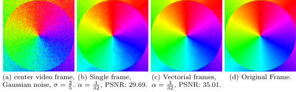
The video underlying Figure 10 is constructed as follows. As basis, we use the image given by the first component of (96) on $[-\tfrac{1}{2},\tfrac{1}{2}]^{2}$ ; outside the disc of radius $\tfrac{1}{2}$ , we add $\tfrac{\pi}{4}$ which is the same as rotating the input $(i,j)$ of each pixel in $\Omega_{0}$ by the same amount clockwise. The video consists of $13$ frames rotating the disc clockwise by $\pi$ and the outer region by $\pi$ counterclockwise, i.e. from $-\tfrac{\pi}{2}$ before the center frame to $\tfrac{\pi}{2}$ at the end of the sequence for the inner and with changed signs for the outer redgion. This corresponds to a rotation of $\tfrac{\pi}{12}$ per frame and region. We finally sample each of these frames with $256\times 256$ pixel on $[-\tfrac{1}{2},\tfrac{1}{2}]^{2}$ .

In our example, Figure 10, we show in (d) the seventh frame of the constructed video from the previous the paragraph. On each frame, we impose wrapped Gaussian noise with standard deviation $\sigma=\frac{2}{5}$ , see Figure 10 (a) for frame 7 of the video. In (b), we perform denoising just on the frame $k=7$ . Performing a first and second order denoising yields staircasing and/or reduction of the sharp edge at the disc border. Choosing the parameters $\alpha=\alpha_{1}=\alpha_{2},\beta=\beta_{1}=\beta_{2}$ from the set $\in\tfrac{1}{64}\mathbb{N}_{0}$ and setting $K=400$ as maximal number of iterations of the CPPA, we obtain the optimal value $\alpha=\tfrac{1}{32}$ , $\beta=0$ . This indicates that staircasing still resembles a better result than unsharpening the edge, which would be the effect of including second order differences. In (c), we perform a combined vectorial denoising in $(\mathbb{S}^{1})^{13}$ as proposed for a total of $13$ frames $(l=6,k=7)$ and show the central seventh frame. At the cost of being computationally more expensive due to the increased data set, this approach outperforms the first, single frame based approach.

Discussion and Future Research

In the following we discuss the relation of the present work to the author’s previous work [6, 7]. These works consider the $\mathbb{S}^{1}$ -valued situation, whereas we here consider the product space $(\mathbb{S}^{1})^{m}\times\mathbb{R}^{n}.$ These product spaces are practically relevant: they appear, e.g., in the context of color space and, more abstractly, whenever considering polar coordinates (magnitude and phase). In contrast to general manifolds the spaces considered here still allow for a solution to the considered minimization problem, i.e. the involved proximal mappings, to be given in explicit form. We are convinced that this is no longer possible for general manifolds. The product spaces further imply changes in both the algorithms and the convergence analysis. Although this paper as well as [6, 7] (and also the previous work [85]) use a CPPA, the derived proximal mappings are different. In particular the mappings derived here do not arise as component-wise application of the one dimensional situation. This is especially not the case for the setting, where several data items are fixed by constraint. In this context, we again mention that the natural second differences on $(\mathbb{S}^{1})^{m}\times\mathbb{R}^{n}$ which we defined in this paper couple the components of the range space, which also affects the convergence analysis The employed methods are based on the ones used in [6] (which themselves are based on [82]), but the concrete analysis involves an additional degree of complexity stemming from the mentioned coupling.

This work also contains material which is even new for $\mathbb{S}^{1}$ -valued data. First, in contrast to pure denoising, additional/different proximal mappings are needed when dealing with the inpainting problem due to the additional constraints. In [7], we simply used the proximal mappings computed in [6] and applied projections to ensure the constraints. Here, we compute the proximal mappings of the constrained problems explicitly. This is more natural and also advantageous in the analysis. Concerning the analysis, we here include an inpainting setup. Even for the $\mathbb{S}^{1}$ setting, this has not yet been done. In the conference proceeding [7] we do not provide a convergence analysis. The paper [6] which provides an analysis considers functionals for denoising in the $\mathbb{S}^{1}$ setting only.

A topic of future research are algorithms for higher order TV-type functionals for data living in more general manifolds.

Acknowledgement.

This research was started when RB visited the Helmholtz-Zentrum München in summer 2014. We thank Gabriele Steidl for valuable discussions. AW is supported by the Helmholtz Association within the young investigator group VH-NG-526. AW also acknowledges the support by the DFG scientific network “Mathematical Methods in Magnetic Particle Imaging”.

References

[1] Marina Almeida and M“’ario Figueiredo “Deconvolving Images With Unknown Boundaries Using the Alternating Direction Method of Multipliers” In IEEE Trans. on Image Process. 22.8, 2013, pp. 3074–3086
[2] Miroslav Ba“’ak “Computing medians and means in Hadamard spaces” In SIAM J. Optim. 24.3, 2014, pp. 1542–1566
[3] Miroslav Ba“’ak “The proximal point algorithm in metric spaces” In Isr. J. Math. 194.2, 2013, pp. 689–701
[4] C. Ballester et al. “Filling in by joint interpolation of vector fields and gray levels” In IEEE Trans. Image Process. 10.8, 2001, pp. 1200–1211
[5] P. Basser, J. Mattiello and D. LeBihan “MR diffusion tensor spectroscopy and imaging” In Biophys. J. 66 Elsevier, 1994, pp. 259–267
[6] R. Bergmann, F. Laus, G. Steidl and A. Weinmann “Second order differences of cyclic data and applications in variational denoising” In SIAM J. Imaging Sci. 7.4, 2014, pp. 2916–2953
[7] Ronny Bergmann and Andreas Weinmann “Inpainting of Cyclic Data using First and Second Order Differences” In EMMCVPR 2015 Springer, 2015, pp. 155–168
[8] Dimitri˜P Bertsekas “Incremental Gradient, Subgradient, and Proximal Methods for Convex Optimization: a Survey”, 2010
[9] Dimitri˜P Bertsekas “Incremental proximal methods for large scale convex optimization” In Math. Program., Ser. B 129.2, 2011, pp. 163–195
[10] R. Bhattacharya and V. Patrangenaru “Large sample theory of intrinsic and extrinsic sample means on manifolds I” In Ann. Statist. 31.1, 2003, pp. 1–29
[11] R. Bhattacharya and V. Patrangenaru “Large sample theory of intrinsic and extrinsic sample means on manifolds II” In Ann. Statist. 33.3, 2005, pp. 1225–1259
[12] P Blomgren and Tony Chan “Color TV: total variation methods for restoration of vector-valued images” In IEEE Trans. Image Process. 7.3, 1998, pp. 304–309
[13] Folkmar Bornemann and Tom M“”arz “Fast image inpainting based on coherence transport” In J. Math. Imaging Vision 28.3, 2007, pp. 259–278
[14] Kristian Bredies, Karl Kunisch and Thomas Pock “Total generalized variation” In SIAM J. Imaging Sci. 3.3, 2010, pp. 492–526
[15] Xavier Bresson and Tony˜F Chan “Fast dual minimization of the vectorial total variation norm and applications to color image processing” In Inverse Probl. Imaging 2.4, 2008, pp. 455–484
[16] Aur“’elie Bugeau, Marcelo Bertalm“’o, Vicent Caselles and Guillermo Sapiro “A comprehensive framework for image inpainting” In IEEE Trans. Signal Process. 19.10, 2010, pp. 2634–2645
[17] Jian-Feng Cai, Raymond˜H Chan and Zuowei Shen “Simultaneous cartoon and texture inpainting” In Inverse Probl. Imaging 19.3, 2010, pp. 379–395
[18] Jian-Feng Cai, Bin Dong, Stanley Osher and Zuowei Shen “Image restoration: Total variation, wavelet frames, and beyond” In J. Amer. Math. Soc. 25.4, 2012, pp. 1033–1089
[19] Vicent Caselles, J-M Morel and Catalina Sbert “An axiomatic approach to image interpolation” In IEEE Trans. Image Process. 7.3, 1998, pp. 376–386
[20] Antonin Chambolle and Pierre-Louis Lions “Image recovery via total variation minimization and related problems” In Numer. Math. 76.2, 1997, pp. 167–188
[21] T˜F Chan, Selim Esedoglu and Frederick˜E Park “Image decomposition combining staircase reduction and texture extraction” In J. Vis. Commun. Image R. 18.6, 2007, pp. 464–486
[22] T.˜F. Chan, S. Kang and J. Shen “Total variation denoising and enhancement of color images based on the CB and HSV color models” In J. Vis. Commun. Image R. 12, 2001, pp. 422–435
[23] T˜F Chan, A Marquina and P Mulet “High-order total variation-based image restoration” In SIAM J. Sci. Comput. 22.2, 2000, pp. 503–516
[24] T.˜F. Chan and J. Shen “Local inpainting models and TV inpainting” In SIAM J. Appl. Math. 62.3, 2001, pp. 1019–1043
[25] Tony˜F Chan and Sung˜Ha Kang “Error analysis for image inpainting” In J. Math. Imaging Vis. 26.1, 2006, pp. 85–103
[26] Tony˜F Chan, Sung˜Ha Kang and Jianhong Shen “Euler’s elastica and curvature-based inpainting” In SIAM J. Appl. Math. 63.2, 2002, pp. 564–592
[27] Tony˜F Chan and Jianhong˜Jackie Shen “Image processing and analysis: variational, PDE, wavelet, and stochastic methods” SIAM, 2005
[28] Tony˜F Chan, Andy˜M Yip and Frederick˜E Park “Simultaneous total variation image inpainting and blind deconvolution” In Int. J. Imag. Syst. Tech. 15.1, 2005, pp. 92–102
[29] C. Chefd’Hotel, D. Tschumperl“’e, R. Deriche and O. Faugeras “Regularizing flows for constrained matrix-valued images” In J. Math. Imaging Vis. 20, 2004, pp. 147–162
[30] S Didas, Gabriele Steidl and Simon Setzer “Combined $\ell_{2}$ data and gradient fitting in conjunction with $\ell_{1}$ regularization” In Adv. Comput. Math. 30.1, 2009, pp. 79–99
[31] S Didas, J Weickert and B Burgeth “Properties of higher order nonlinear diffusion filtering” In J. Math. Imaging Vis. 35, 2009, pp. 208–226
[32] Bin Dong et al. “Wavelet frame based blind image inpainting” In Appl. Comput. Harmon. Anal. 32.2, 2012, pp. 268–279
[33] Michael Elad, J-L Starck, Philippe Querre and David˜L Donoho “Simultaneous cartoon and texture image inpainting using morphological component analysis (MCA)” In Appl. Comput. Harmon. Anal. 19.3 Elsevier, 2005, pp. 340–358
[34] Selim Esedoglu and Jianhong Shen “Digital inpainting based on the Mumford–Shah–Euler image model” In European J. of Appl. Math. 13.4 Cambridge Univ Press, 2002, pp. 353–370
[35] O.˜P. Ferreira and P.˜Roberto Oliveira “Proximal point algorithm on Riemannian manifolds” In Optimization 51.2, 2002, pp. 257–270
[36] N˜I Fisher “Statistical Analysis of Circular Data” Cambridge University Press, 1996
[37] P Fletcher “Geodesic regression and the theory of least squares on Riemannian manifolds” In Int. J. Comput. Vis. 105.2, 2013, pp. 171–185
[38] Mariano Giaquinta, Giuseppe Modica and Jaroslav Souek “Variational problems for maps of bounded variation with values in $S^{1}$ ” In Calc. Var. 1.1, 1993, pp. 87–121
[39] Mariano Giaquinta and Domenico Mucci “Maps of bounded variation with values into a manifold: total variation and relaxed energy” In Pure Appl. Math. Q. 3.2, 2007, pp. 513–538
[40] Mariano Giaquinta and Domenico Mucci “The BV-energy of maps into a manifold: relaxation and density results” In Ann. Sc. Norm. Super. Pisa 5.4, 2006, pp. 483–548
[41] Bastian Goldluecke, E Strekalovskiy and Daniel Cremers “Tight Convex Relaxations for Vector-Valued Labeling” In SIAM J. Imaging Sci. 6.3, 2013, pp. 1626–1664
[42] Bastian Goldluecke, Evgeny Strekalovskiy and Daniel Cremers “The natural vectorial total variation which arises from geometric measure theory” In SIAM J. Imaging Sci. 5.2, 2012, pp. 537–563
[43] P. Grohs, H. Hardering and O. Sander “Optimal A Priori Discretization Error Bounds for Geodesic Finite Elements” to appear In Found. Comput. Math., 2015
[44] Philipp Grohs and Johannes Wallner “Interpolatory wavelets for manifold-valued data” In Appl. Comput. Harmon. Anal. 27.3, 2009, pp. 325–333
[45] Christine Guillemot and Olivier Le˜Meur “Image inpainting: Overview and recent advances” In IEEE Signal Processing Mag. 31.1 IEEE, 2014, pp. 127–144
[46] Stanislav Harizanov, Peter Oswald and Tatiana Shingel “Normal multi-scale transforms for curves” In Foundations of Computational Mathematics 11.6 Springer, 2011, pp. 617–656
[47] Allen Hatcher “Algebraic Topology” Cambridge University Press, 2002
[48] Walter Hinterberger and Otmar Scherzer “Variational methods on the space of functions of bounded Hessian for convexification and denoising” In Computing 76.1, 2006, pp. 109–133
[49] S˜R Jammalamadaka and A SenGupta “Topics in Circular Statistics” World Scientific Publishing Company, 2001
[50] R. Kimmel and N. Sochen “Orientation diffusion or how to comb a porcupine” In J. Vis. Commun. Image R. 13.1–2 Elsevier, 2002, pp. 238–248
[51] Emily˜J King, Gitta Kutyniok and Xiaosheng Zhuang “Analysis of inpainting via clustered sparsity and microlocal analysis” In J. Math. Imaging Vis. 48.2 Springer, 2014, pp. 205–234
[52] R. Lai and S. Osher “A splitting method for orthogonality constrained problems” In J. Sci. Comput. 58.2 Springer, 2014, pp. 431–449
[53] S Lefkimmiatis, A Bourquard and M Unser “Hessian-Based Norm Regularization for Image Restoration With Biomedical Applications” In IEEE Trans. Image Process. 21.3, 2012, pp. 983–995
[54] J Lellmann, E Strekalovskiy, S Koetter and D Cremers “Total variation regularization for functions with values in a manifold” In IEEE ICCV 2013, 2013, pp. 2944–2951
[55] M Lysaker, A Lundervold and Xue-Cheng Tai “Noise removal using fourth-order partial differential equations with applications to medical magnetic resonance images in space and time” In IEEE Trans. Image Process. 12.12, 2003, pp. 1579–1590
[56] Marius Lysaker and Xue-Cheng Tai “Iterative image restoration combining total variation minimization and a second-order functional” In Int. J. Comput. Vis. 66.1, 2006, pp. 5–18
[57] Thomas M“”arz “A well-posedness framework for inpainting based on coherence transport” In Found. Comput. Math. 15, 2013, pp. 973–1033
[58] Thomas M“”arz “Image inpainting based on coherence transport with adapted distance functions” In SIAM J. Imaging Sci. 4.4 SIAM, 2011, pp. 981–1000
[59] Simon Masnou “Disocclusion: a variational approach using level lines” In IEEE Trans. Image Process. 11.2 IEEE, 2002, pp. 68–76
[60] Simon Masnou and J-M Morel “Level lines based disocclusion” In IEEE ICIP 1998, 1998, pp. 259–263
[61] Thomas M“”ollenhoff, E Strekalovskiy, Michael M“”oller and Daniel Cremers “Low Rank Priors for Color Image Regularization” In EMMCVPR 2015 Springer, 2015, pp. 126–140
[62] J. Oller and J. Corcuera “Intrinsic analysis of statistical estimation” In Ann. Statist. 23.5 JSTOR, 1995, pp. 1562–1581
[63] K. Papafitsoros and C.B. Schönlieb “A Combined First and Second Order Variational Approach for Image Reconstruction” In Journal of Mathematical Imaging and Vision 48.2, 2014, pp. 308–338 DOI: 10.1007/s10851-013-0445-4
[64] Konstantinos Papafitsoros, Carola˜Bibiane Schoenlieb and Bati Sengul “Combined First and Second Order Total Variation Inpainting using Split Bregman” In Image Processing On Line 3, 2013, pp. 112–136 DOI: 10.5201/ipol.2013.40
[65] X. Pennec, P. Fillard and N. Ayache “A Riemannian framework for tensor computing” In Int. J. Comput. Vis. 66.1 Springer, 2006, pp. 41–66
[66] Xavier Pennec “Intrinsic Statistics on Riemannian Manifolds: Basic Tools for Geometric Measurements” In J. Math. Imaging Vis. 25.1, 2006, pp. 127–154
[67] Lars˜Lau Rak“ˆet, Lars Roholm, Mads Nielsen and Francois Lauze “TV- $L^{1}$ optical flow for vector valued images” In EMMCVPR 2011, 2011, pp. 329–343 Springer
[68] R˜T Rockafellar “Monotone operators and the proximal point algorithm” In SIAM J. Control Optim. 14.5, 1976, pp. 877–898
[69] G. Rosman et al. “Group-valued regularization framework for motion segmentation of dynamic non-rigid shapes” In SSVM 2011, LNCS 6667 Springer, 2012, pp. 725–736
[70] Leonid˜I Rudin, Stanley Osher and Emad Fatemi “Nonlinear total variation based noise removal algorithms” In Physica D. 60.1, 1992, pp. 259–268
[71] O Scherzer “Denoising with higher order derivatives of bounded variation and an application to parameter estimation” In Computing 60, 1998, pp. 1–27
[72] Simon Setzer and Gabriele Steidl “Variational methods with higher order derivatives in image processing” In Approximation XII: San Antonio 2007, 2008, pp. 360–385
[73] Simon Setzer, Gabriele Steidl and T Teuber “Infimal convolution regularizations with discrete l1-type functionals” In Commun. Math. Sci. 9.3, 2011, pp. 797–872
[74] Jianhong Shen and Tony˜F Chan “Mathematical models for local nontexture inpaintings” In SIAM J. Appl. Math. 62.3, 2002, pp. 1019–1043
[75] E Strekalovskiy and Daniel Cremers “Total Cyclic Variation and Generalizations” In J. Math. Imaging Vis. 47.3, 2013, pp. 258–277
[76] E Strekalovskiy and Daniel Cremers “Total variation for cyclic structures: Convex relaxation and efficient minimization” In IEEE CVPR 2011, 2011, pp. 1905–1911
[77] D. Tschumperl“’e and R. Deriche “Diffusion tensor regularization with constraints preservation” In IEEE CVPR 2001 1, 2001, pp. 948–953
[78] David Tschumperl“’e “Fast anisotropic smoothing of multi-valued images using curvature-preserving PDE’s” In Int. J. Comput. Vis. 68.1 Springer, 2006, pp. 65–82
[79] I. Ur˜Rahman et al. “Multiscale representations for manifold-valued data” In Multiscale Model. and Sim. 4 SIAM, 2005, pp. 1201–1232
[80] Tuomo Valkonen, Kristian Bredies and Florian Knoll “Total Generalized Variation in Diffusion Tensor Imaging” In SIAM J. Imaging Sci. 6.1, 2013, pp. 487–525
[81] L. Vese and S. Osher “Numerical methods for p-harmonic flows and applications to image processing” In SIAM J. Numer. Anal. 40.6, 2002, pp. 2085–2104
[82] J. Wallner and N. Dyn “Convergence and $C^{1}$ analysis of subdivision schemes on manifolds by proximity” In Comput. Aided Geom. D. 22 Elsevier, 2005, pp. 593–622
[83] A. Weinmann “Interpolatory multiscale representation for functions between manifolds” In SIAM J. Math. Anal. 44 SIAM, 2012, pp. 162–191
[84] Andreas Weinmann “Nonlinear subdivision schemes on irregular meshes” In Constr. Approx. 31.3 Springer, 2010, pp. 395–415
[85] Andreas Weinmann, Laurent Demaret and Martin Storath “Total variation regularization for manifold-valued data” In SIAM J. Imaging Sci. 7.4, 2014, pp. 2226–2257