Nonlinear spin diffusion and spin rotation in a trapped Fermi gas

Transverse spin diffusion occurs when the magnetization is oriented along different directions, for instance, in a spin helix. It has been observed in spin-echo experiments in helium [1], polarized hydrogen, and, recently, ultracold atomic gases [2, 3, 4]. The transverse magnetization evolves according to a diffusion equation, but there are additional terms from the precession of the spin currents around the local magnetization. This Leggett-Rice effect [5, *leggett1970] is related to the identical spin-rotation effect [7, *miyake1985] and leads to reactive spin currents and spin waves, which have been observed in ultracold Fermi gases [9, *du2009, *heinze2013]. Consider a polarized sample with small transverse magnetization (small tipping angle). The transverse magnetization is conveniently combined into a complex number $m_{+}=m_{x}+im_{y}$, which evolves with a complex diffusion coefficient,

where $D_{0}^{\perp}$ is the transverse diffusivity and $\mu m_{z}=\gamma$ (at full polarization) the dimensionless spin-rotation parameter. For small $\mu\to 0$ this is the usual diffusion equation, while for large $\lvert\mu\rvert$ the diffusion equation has an imaginary effective diffusivity and resembles the Schrödinger equation [12]. In a spin-echo pulse sequence, the second term in Eq. (1) expresses a linear gradient $\alpha$ of the external magnetic field along the $x_{3}$ direction, which winds the magnetization into a helix. After a time $t_{\pi}$, a $\pi$ pulse is applied, which is equivalent to flipping the sign of $\alpha$. In the ensuing time evolution, the helix unwinds until the magnetization is realigned at the echo time $t_{e}=2t_{\pi}$. In the presence of spin rotation $\mu\neq 0$, realignment at $t_{e}$ occurs at a phase angle $\phi\propto\mu$ with respect to the initial orientation at $t=0$ [5, *leggett1970], and the value of $\mu$ can be inferred. For a strongly interacting Fermi gas the value of $\mu$ has recently been measured and used to determine the spin-antisymmetric Fermi-liquid parameter $F_{1}^{a}$, while the sign of $\mu$ reveals the attractive or repulsive character of the effective interaction [4]. Theoretically, $D_{0}^{\perp}$ and $\mu$ for dilute, homogeneous Fermi gases have been computed using kinetic theory [13, *jeon1989, *mullin1992, 16].

In an infinite homogeneous system where the only position dependence arises from the magnetic field gradient $\alpha$, the phase angle $\phi$ is directly proportional to the microscopic parameter $\mu$. Instead, for a finite homogeneous box the phase $\phi$, and hence the apparent value of $\mu$, saturates when the system size is reached [17]. Experiments with ultracold atomic gases typically employ a harmonic trapping potential which is both finite and inhomogeneous: in this case, the diffusivity $D_{0}^{\perp}$, the Leggett-Rice parameter $\mu$, and the magnetization $m_{z}$ are strongly position dependent, and the diffusion equation (1) becomes nonlinear. In previous studies the evolution has been linearized in order to determine the collective mode frequencies and decay rates in the trapping potential [18, *ragan2004leggett, *mullin2006]. Other studies consider the nonlinear evolution of the full phase-space distribution for a nondegenerate or collisionless trapped gas [21, *piechon2009]. Here, I numerically solve the nonlinear evolution equation with position dependent kinetic coefficients including medium scattering to obtain the transverse magnetization decay and the growth of the phase $\phi$ for the specific trap geometry used in the experiment.

Kinetic theory [23] is employed to compute the spin evolution of the trapped gas. This method is well controlled in the weak-coupling limit, which is also the parameter regime where finite-size corrections due to the trapping potential are most pronounced [4]. On the other hand, at strong coupling toward unitarity and at low temperature near the superfluid phase transition of an attractive Fermi gas [24], kinetic theory is expected to receive quantitative corrections from the effects of pairing and short quasiparticle lifetimes, which are incorporated for instance when computing transport from the Kubo formula within a Luttinger-Ward approach [25, *bauer2014, 27].

This paper is structured as follows: in Sec. II the spin evolution equations for a trapped Fermi gas are derived from kinetic theory, while Sec. III compares them to the known homogeneous limit. Section IV presents the results for the magnetization profiles and apparent diffusivities, and Sec. V concludes with a discussion.

Transport in an interacting Fermi gas may be described by kinetic theory for quasiparticles, as long as they are sufficiently long-lived. For a multi-component Fermi gas with two or more spin species one has to compute the time evolution of the spin distribution $\underline{n}_{p}$, which is a matrix with components $\underline{n}_{p}=n_{p\sigma\sigma^{\prime}}(\bm{x},t)$ in spin space. The evolution equation derived by Landau and Silin [28, 29] reads

where $\underline{\varepsilon}_{p}=\varepsilon_{p\sigma\sigma^{\prime}}(\bm{x},t)$ is the matrix of single-particle energies. The left-hand side constitutes the drift term, while the right-hand side describes the change in the distribution caused by collisions. Specifically for the spin-$1/2$ case, $\underline{n}_{p}$ and $\underline{\varepsilon}_{p}$ are $2\times 2$ matrices in spin space, for instance, in the $\uparrow$, $\downarrow$ basis.

The spin matrices can be decomposed in terms of the identity $\underline{I}$ and the Pauli matrices $\underline{\bm{\sigma}}$. The occupation number matrix is written as

where $f_{p}(\bm{x},t)$ is the particle number distribution function and $\bm{\sigma}_{p}(\bm{x},t)$ the spin vector distribution in Bloch space. Similarly, the energy matrix

combines the spin-independent single-particle energies $\varepsilon_{p}(\bm{x},t)$ and a magnetic field $\bm{h}_{p}(\bm{x},t)$. One may then rewrite Eq. (2) as

and

The spin-rotation term $\bm{h}_{p}\times\bm{\sigma}_{p}$ is responsible for the Leggett-Rice effect. The single-particle energies are

for a Fermi gas in a harmonic trapping potential $V(\bm{x})$, which can be anisotropic with different trapping frequencies $\omega_{j}$ in spatial direction $j$. The magnetic field

is written in terms of the Larmor frequency $\bm{\Omega}=\bm{\Omega}_{0}+\bm{\Omega}_{\text{mf}}$. For a spin-echo protocol it has two contributions: $(i)$ $\bm{\Omega}_{0}=\gamma\bm{B}(\bm{x},t)$ is due to the external magnetic field $\bm{B}(\bm{x},t)$ with gyromagnetic ratio $\gamma$. A spatially constant $\bm{B}$ is compensated by going to the co-rotating frame in Bloch space, but a magnetic field $B_{z}$ gradient of slope $\alpha$ along the $x_{3}$ direction winds up the local magnetization into a spin spiral. $(ii)$ The second contribution to the Larmor frequency, $\bm{\Omega}_{\text{mf}}$, is a mean-field term proportional to the local magnetization ${\bm{m}}$ of a polarized Fermi gas. It leads to the precession of the spin current around ${\bm{m}}$.

The evolution of the full distribution functions $f_{p}(\bm{x},t)$ and $\bm{\sigma}_{p}(\bm{x},t)$ is simplified by considering moments with respect to momentum:

with bare velocity $v_{pj}=\partial\varepsilon_{p}/\partial p_{j}=p_{j}/m$. An additional contribution $f_{p}\partial\bm{h}_{p}/\partial p_{j}$ to the spin current is absent for momentum-independent $\bm{h}_{p}$. The local polarization is defined as $\bm{M}(\bm{x},t)={\bm{m}}(\bm{x},t)/n(\bm{x},t)$ where $\lvert\bm{M}(\bm{x},t)\rvert\leq 1$. The spin current ${\bm{J}}_{j}$ is both a vector in Bloch space (bold symbol) and a vector in position space ($j$ index): it encodes how the magnetization changes as one goes along the $j$ direction. The evolution equations for the moments read, using the specific form of the single-particle energies (7)–(9),

The projectors $P_{\parallel}\bm{a}\equiv(\bm{a}\cdot\hat{{\bm{m}}})\hat{{\bm{m}}}$ and $P_{\perp}\equiv 1-P_{\parallel}$ give the component of the magnetization gradient parallel and perpendicular to the local magnetization, respectively. When deriving these equations, the mean field $\bm{\Omega}_{\text{mf}}$ has been retained only in the spin-rotation term and not in the Poisson brackets in Eqs. (5) and (6). This can be justified as the leading order in a controlled large-$N$ expansion [30]. In general, the evolution of the currents depends on the second moments of $f_{p}$ and $\bm{\sigma}_{p}$ which in turn depend on higher moments. However, near local equilibrium the linearized Boltzmann equation relates the higher moments to the lower ones via the coefficients $\alpha_{n}$, $\tau_{n}$, $\alpha_{\parallel,\perp}$, $\tau_{D}$, and $W$, and one obtains a closed set of evolution equations. These coefficients are discussed in Sec. II.2.

The evolution equations (14)–(17) leave the density profile largely invariant, but the spin distribution changes dramatically as the magnetization is wound up into a helix according to the equations

The full numerical solution of these equations is presented in Sec. IV. In order to gain a qualitative understanding of the spin evolution in a trapped gas, it is instructive to consider first the approximate analytical solutions in the homogeneous case.

If the scattering time $\tau_{D}$ is much shorter than any other relevant time scale, for instance, the dephasing time $\tau=(D^{\perp}\alpha^{2})^{-1/3}$ due to the helix, the current reaches a steady state and its time derivative vanishes in the rotating frame, $\partial_{t}\bm{J}_{j}=-\alpha x_{3}\hat{\bm{z}}\times\bm{J}_{j}$. Defining $D_{0}^{\perp}=\alpha_{\perp}\tau_{D}$ and $\mu{\bm{m}}=-\tau_{D}\bm{\Omega}_{\text{mf}}=\gamma\bm{M}$ one finds

This equation is solved by the steady-state current

where $D_{0}^{\perp}$, $\mu$, and $\tau_{D}$ may still depend on position; the last term arises due to the trapping potential. Inserting this current into the continuity equation for the magnetization (33) yields

The Leggett solution [5, *leggett1970] is recovered in the homogeneous limit $\omega_{j}=0$, where ${\bm{m}}^{2}$ remains constant in space:

In this case the longitudinal magnetization $m_{z}$ remains unchanged, while the transverse magnetization $m_{+}=m_{x}+im_{y}$ evolves as

with effective diffusivity $D_{\text{eff}}^{\perp}=D_{0}^{\perp}/(1+\mu^{2}{\bm{m}}^{2})$. Since ${\bm{m}}^{2}$ is constant in space, this is now a linear diffusion equation, albeit with a complex diffusion coefficient.

In the spin-echo protocol, the gradient $\alpha$ winds up the transverse magnetization $m_{+}=m_{x}+im_{y}$ into a helix along the $x_{3}$ direction. A transverse spin current $J_{3+}\sim\partial_{3}m_{+}$ appears, which tends to smooth the helix. If $J_{3+}$ has a component perpendicular to the local magnetization ${\bm{m}}\approx m_{z}\hat{\bm{z}}$ (at small tipping angle) it precesses around it at frequency $\Omega_{\text{mf}}=Wm_{z}/\hbar$. At time $t_{\pi}$, a $\pi$ pulse around the $y$ axis in Bloch space is applied; this is equivalent to reversing the sign of $\alpha$. The subsequent time evolution unwinds the helix until the echo time $t_{e}=2t_{\pi}$, where the transverse magnetization is again homogeneous. In the absence of spin rotation, $\gamma=0$, the modulus of the transverse magnetization $A(t)=\lvert m_{+}(t)\rvert$ at time $t_{e}$ decays as a cubic exponential [5, *leggett1970]

where $A_{0}=A(0)$. This result is approximately correct even for $\gamma\neq 0$ if the tipping angle $\theta$ is small, $\lvert m_{+}\rvert\ll\lvert m_{z}\rvert$, and for short times. For finite $\gamma$, the magnetization decay is slowed down and is given by [4]

where $\eta=\gamma^{2}(A_{0}/n)^{2}/(1+\gamma^{2}M_{z}^{2})$ for polarization $M_{z}$, and $\mathcal{W}(z)$ is the Lambert-$W$ function. This solution for the homogeneous system is used in the analysis of the experimental data to fit the diffusivity $D_{0}^{\perp}$ and the apparent Leggett-Rice parameter $\gamma$ from the measured magnetization decay and phase shift $\phi$ of the trapped system. In the following the full spin evolution in the trap is computed explicitly to determine to what extent the homogeneous solution is still applicable to the trapped gas.

In the trapped gas, the assumptions which led to the analytical solutions in Sec. III (steady-state current, homogeneity) are not satisfied. Instead, a full numerical solution of the spin evolution equations, (33) and (34), is necessary. The initial condition in the experimental protocol [4] is a fully polarized cloud of fermionic atoms with a thermal profile, (19) and (22), for tipping angle $\theta$. This distribution is stationary in the absence of an external magnetic field gradient $\alpha$. Due to the density profile, (19), also the coefficients $\alpha_{\perp}(\bm{x})$, $\tau_{\perp}(\bm{x})$, and $W(\bm{x})$ depend on the position in the trap. For a small tipping angle $\lvert m_{+}\rvert\ll\lvert m_{z}\rvert$ the gas remains almost fully polarized, hence the density profile and the coefficients are time independent even in the presence of the gradient $\alpha$.

In the numerical solution, the experimental parameters [4] are used: gradient $\alpha=1.67\mu$m^-1kHz, trap frequency $\omega_{3}=2\pi\times 750$ Hz, $\bar{\omega}=2\pi\times 470$ Hz, roughly $N\sim 40000$ atoms of ⁴⁰K with a Fermi energy of $E_{F}=2\pi\hbar\times 29$ kHz, and Thomas-Fermi radius $R_{TF}=5.1\mu$m. Even though the Fermi gas is initially fully polarized, the Fermi wave vector $k_{F}=12\mu$m^-1 and the Fermi time $\tau_{F}=0.0087$ ms are taken for a hypothetical balanced gas of the same atom number in order to recover the standard relation $n=k_{F}^{3}/3\pi^{2}$ for the total density [4]. At the lowest experimental temperature, $T\approx 280$ nK, the initial reduced temperature is $(T/T_{F})_{i}=0.2$ and $\lambda=0.52\mu$m. The phase-space density at the trap center reaches $\lambda^{3}n=7.3$, well within the quantum degenerate regime.

In Fig. 2, the helical state of the local magnetization in the trap at $1/k_{F}a=-2$ is shown for different times $t_{\pi}$ (left column). At this time, the $\pi$ pulse is applied (equivalently, the sign of $\alpha$ is reversed), and the subsequent time evolution unwinds the helix until the echo time $t_{e}=2t_{\pi}$ (right column), which is chosen between $t_{e}=0.2$ ms and $t_{e}=1.2$ ms. For comparison, the density profiles for a homogeneous gas with $t_{e}=1.2$ ms are shown as dashed lines. At time $t_{\pi}$, the $\phi$ profiles of the trapped and the homogeneous gas have a similar slope and are shifted toward negative phase angles by spin rotation. At time $t_{e}$, instead, the phase angle of the homogeneous gas is again homogeneous, but $m_{+}$ for the trapped gas remains in a helical state. Therefore, the trap-averaged transverse magnetization decays quickly even though the local $m_{+}$ is still sizable, and the apparent slope $\phi(t_{e})/M_{z}\ln(A(t_{e})/A_{0})$ is lower than in the homogeneous case, where it reaches the microscopic value $\gamma=-Wm_{z}\tau_{D}/\hbar$ according to Eq. (40). As we see below, this effect leads to a saturation of the apparent $\gamma$ for weak coupling.

Note that the magnetization profiles are not symmetric with respect to $x_{3}$: this is due to the spin-rotation term in Eq. (37) producing an additional phase shift on top of the gradient $\alpha$. Consequently, if one reverses the sign of the scattering length $a$, the sign of $\gamma$ is approximately reversed, and the resulting magnetization profile is the mirror image with $x_{3}\mapsto-x_{3}$. Note also that at strong coupling $1/k_{F}a=0$, the phase profile at $t_{e}$ is nearly homogeneous at the trap center (not shown), and the kinetic coefficients for the trapped gas approach those in the homogeneous case.

Figure 3 shows the decay of the trap-averaged transverse magnetization with time (left column), and the growth of the phase angle $\phi$ with the slope of the magnetization decay (right column). From these plots, the apparent Leggett-Rice parameter $\gamma=\phi(t_{e})/M_{z}\ln(A(t_{e})/A_{0})$ can be read off as the slope of the curve through the origin. This value of $\gamma$ is then used to fit the magnetization decay on the left side of Fig. 3 to the analytical decay function (39) with diffusivity $D_{0}^{\perp}$. Here, I follow the analysis of the experimental data in Ref. 4 and fit the decay of the trapped gas to the homogeneous solution.

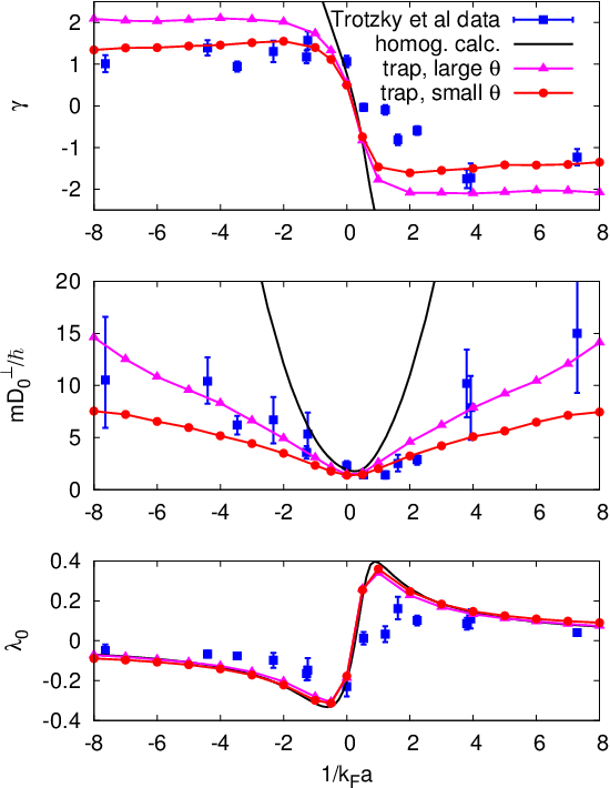
In Fig. 4, the apparent Leggett-Rice parameter $\gamma$ extracted above is plotted versus the interaction strength, from the BCS regime (left) via unitarity ($1/k_{F}a=0$) to the repulsive branch (right). For a trapped gas, I find that the apparent $\gamma$ saturates for weak coupling on both the BCS and the repulsive sides. This behavior differs qualitatively from the homogeneous case, where $\gamma$ continues to increase linearly at weak coupling [cf. Eq. (32)] (solid black line). The trap calculation thus explains the saturation of $\gamma$ observed in experiments [4]. The absolute value of $\gamma$ for the trapped gas depends on the tipping angle $\theta$ of the initial polarization: for a large tipping angle $\theta=\pi/3$ as in the experiment, the Leggett-Rice parameter $\gamma$ saturates at larger values than in the case of a small tipping angle $\theta=\pi/30$. The value to which $\gamma$ saturates also depends on the strength of the gradient $\alpha$, in contrast to the homogeneous case (see below). Figure 4 also shows that the Leggett-Rice parameter changes sign, reflecting the sign of the effective interaction between quasiparticles which is attractive on the BCS side and repulsive on the repulsive branch [4]. The sign change occurs for slightly positive values of $1/k_{F}a$.

The center panel in Fig. 4 shows the bare transverse diffusivity $D_{0}^{\perp}$. Again, the trap diffusivity is significantly lower than the homogeneous value (solid black line) at weak coupling and agrees with experiment. Once $\gamma$ is known, the bare diffusivity $D_{0}^{\perp}$ is found from the fit of the analytical solution (39) to the magnetization decay in Fig. 3.

The bottom panel in Fig. 4 displays the ratio

It measures the strength of the effective interaction irrespective of the scattering time $\tau_{D}$ and follows the sign change of $\gamma$ since $D_{0}^{\perp}>0$. Again, the trap calculation agrees with the experimental data except in the instability region $0<1/k_{F}a\lesssim 1.3$ [4], while the homogeneous gas has more pronounced interaction effects.

Spin rotation in a trapped gas is determined qualitatively by the ratio between different length scales: the trap size $R_{\text{TF}}\approx 5\mu$m, the helix pitch $\ell_{\text{helix}}=2\pi/(\alpha t_{e}/2)\approx 4\mu$m for $t_{e}=2$ ms, and the mean free path $\ell_{\text{mfp}}=v_{F}\tau_{D}$, which ranges from $0.5\mu$m at unitarity to $3.8\mu$m at $1/k_{F}a=-2$. In simulations with a gradient $\alpha$ larger than the experimental value, several helix pitches fit into the trap, $R_{\text{TF}}\gg\ell_{\text{helix}}$, and the trap averaged diffusivity and $\gamma$ are equal to their homogeneous values as long as also $\ell_{\text{mfp}}<\ell_{\text{helix}}$, but saturate for larger $\ell_{\text{mfp}}$. This is in marked contrast to longitudinal spin diffusion, where a scaling factor of about $5$ was found to relate the trap-averaged and homogeneous diffusivity $D_{\parallel}$ [35, 33, *bruun2011spin, 27]. For weaker gradients where $\ell_{\text{helix}}>R_{\text{TF}}$, less than one helix pitch fits into the trap and the homogeneous solution is reached not even at unitarity where $R_{\text{TF}}\gg\ell_{\text{mfp}}$.

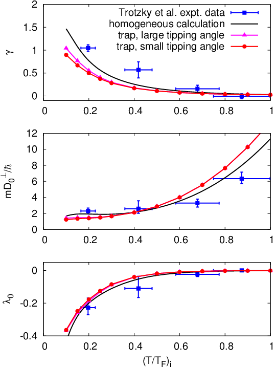
Finally, Fig. 5 shows the temperature dependence of the Leggett-Rice parameter at unitarity. $\gamma$ decreases with temperature, which is understood as follows: the two-body scattering amplitude is purely imaginary at unitarity and would imply a vanishing $\gamma\sim\Re{\mathcal{T}}$. Hence, the observed finite value of $\gamma$ in the quantum degenerate regime $(T/T_{F})_{i}<1$ is a many-body effect due to medium scattering. The presence of the medium enhances both the dissipative and the reactive effects of scattering at low temperatures, and more so in the homogeneous gas than in the trap, where only the core is strongly interacting.

Similarly, the diffusivity reaches values of $D_{0}^{\perp}\simeq 2\hbar/m$ in the quantum degenerate regime (center panel), in agreement with experiment, while the ratio $\lambda_{0}$ becomes large only at the lowest temperatures (lower panel).

To summarize, a spin-echo sequence in a trapped Fermi gas is modeled by a nonlinear and complex diffusion equation for the transverse magnetization. The spin evolution exhibits the Leggett-Rice effect of strength $\gamma=\mu n$, which appears to saturate for weak coupling, and a bare diffusivity much lower than expected for a homogeneous gas of the same temperature and interaction strength. These results are obtained without any fit parameters and agree very well with the weak-coupling data measured recently for a trapped gas of ultracold fermionic ⁴⁰K atoms [4]. The present calculation provides an intuitive interpretation of the observed saturation of $\gamma$: while the spin helix in the homogeneous gas is completely unwound at the echo time $t_{e}$, the trapped gas remains partially in a helical state, with the average transverse magnetization $A(t_{e})$ strongly reduced and a smaller phase shift $\phi(t_{e})$. At weak coupling $1/\lvert k_{F}a\rvert\gtrsim 2$ the kinetic theory employed in this study is well controlled and includes the relevant interaction effects.

At strong coupling $1/k_{F}a=0$ (unitarity), the Leggett-Rice effect is absent at the two-body level and arises only due to many-body medium scattering. The trap calculation at strong coupling agrees with the experimental results qualitatively; the remaining differences may be due to reheating in a demagnetized Fermi gas [3, 4] or due to interaction corrections to the equation of state which were not included in this study; they remain a topic for future work.

Ultracold Fermi gases are thus ideal systems to study the interaction and temperature dependence of the Leggett-Rice effect and the spin transport coefficients. The spin dynamics of the trapped gas (Fig. 2) is much more complex than in the homogeneous case and requires a numerical solution. The spin evolution simplifies near unitarity if $R_{\text{TF}}>\ell_{\text{helix}}>\ell_{\text{mfp}}$, in which case the homogeneous solution is recovered without any trap-related scaling factors. The decay of the trap-averaged magnetization can be analyzed by the methods developed for the homogeneous case: the magnetization decay fits the homogeneous solution surprisingly well (Fig. 3). This study shows that the extracted transport coefficients for the trapped gas can differ markedly, especially at weak coupling, from those of the corresponding homogeneous system (Fig. 4). Conveniently for the interpretation, the sign of $\gamma$, which reveals the repulsive or attractive character of the effective interaction, does not change with the trap average.

The author wishes to thank E. Taylor, J. Thywissen, S. Trotzky, and S. Zhang for stimulating discussions.

References

- [1] E. L. Hahn, “Spin Echoes,” Phys. Rev. 80, 580 (1950).
- [2] M. Koschorreck, D. Pertot, E. Vogt, and M. Köhl, “Universal spin dynamics in two-dimensional Fermi gases,” Nat. Phys. 9, 405 (2013).
- [3] A. B. Bardon, S. Beattie, C. Luciuk, W. Cairncross, D. Fine, N. S. Cheng, G. J. A. Edge, E. Taylor, S. Zhang, S. Trotzky, and J. H. Thywissen, “Transverse Demagnetization Dynamics of a Unitary Fermi Gas,” Science 344, 722 (2014).
- [4] S. Trotzky, S. Beattie, C. Luciuk, S. Smale, A. B. Bardon, T. Enss, E. Taylor, S. Zhang, and J. H. Thywissen, “Observation of the Leggett-Rice Effect in a Unitary Fermi Gas,” Phys. Rev. Lett. 114, 015301 (2015).
- [5] A. J. Leggett and M. J. Rice, “Spin Echoes in Liquid He3 and Mixtures: A Predicted New Effect,” Phys. Rev. Lett. 20, 586 (1968).
- [6] A. J. Leggett, “Spin diffusion and spin echoes in liquid 3He at low temperature,” J. Phys. C 3, 448 (1970).
- [7] C. Lhuillier and F. Laloë, “Transport properties in a spin polarized gas,” J. Phys. (Paris) 43, 197 (1982).
- [8] K. Miyake, W. J. Mullin, and P. C. E. Stamp, “Mean-field and spin-rotation phenomena in Fermi systems: the relation between the Leggett-Rice and Lhuillier-Laloë effects,” J. Phys. (Paris) 46, 663 (1985).
- [9] X. Du, L. Luo, B. Clancy, and J. E. Thomas, “Observation of Anomalous Spin Segregation in a Trapped Fermi Gas,” Phys. Rev. Lett. 101, 150401 (2008).
- [10] X. Du, Y. Zhang, J. Petricka, and J. E. Thomas, “Controlling Spin Current in a Trapped Fermi Gas,” Phys. Rev. Lett. 103, 010401 (2009).
- [11] J. Heinze, J. S. Krauser, N. Fläschner, K. Sengstock, C. Becker, U. Ebling, A. Eckardt, and M. Lewenstein, “Engineering Spin Waves in a High-Spin Ultracold Fermi Gas,” Phys. Rev. Lett. 110, 250402 (2013).
- [12] L. P. Lévy and A. E. Ruckenstein, “Collective Spin Oscillations in Spin-Polarized Gases: Spin-Polarized Hydrogen,” Phys. Rev. Lett. 52, 1512 (1984).
- [13] J. W. Jeon and W. J. Mullin, “Kinetic equation for dilute, spin-polarized quantum systems,” J. Phys. (Paris) 49, 1691 (1988).
- [14] J. W. Jeon and W. J. Mullin, “Transverse spin diffusion in polarized Fermi gases,” Phys. Rev. Lett. 62, 2691 (1989).
- [15] W. J. Mullin and J. W. Jeon, “Spin diffusion in dilute, polarized 3He-4He solutions,” J. Low Temp. Phys. 88, 433 (1992).
- [16] T. Enss, “Transverse spin diffusion in strongly interacting Fermi gases,” Phys. Rev. A 88, 033630 (2013).
- [17] O. Buu, R. Nyman, R. M. Bowley, and J. R. Owers-Bradley, “Leggett-Rice effect in a finite geometry,” Phys. Rev. B 65, 134512 (2002).
- [18] R. J. Ragan, “Spin-rotation effects in bounded spin diffusion,” J. Low Temp. Phys. 98, 489 (1995).
- [19] R. J. Ragan and J. Baggett, “Leggett-Rice Systems in Harmonic Traps,” J. Low Temp. Phys. 134, 369 (2004).
- [20] W. J. Mullin and R. J. Ragan, “Spin diffusion in trapped gases: Anisotropy in dipole and quadrupole modes,” Phys. Rev. A 74, 043607 (2006).
- [21] J.-N. Fuchs, D. M. Gangardt, and F. Laloë, “Large amplitude spin waves in ultra-cold gases,” Eur. Phys. J. D 25, 57 (2003).
- [22] F. Piéchon, J.-N. Fuchs, and F. Laloë, “Cumulative Identical Spin Rotation Effects in Collisionless Trapped Atomic Gases,” Phys. Rev. Lett. 102, 215301 (2009).
- [23] H. Smith and H. H. Jensen, Transport Phenomena (Oxford University Press, Oxford, UK, 1989).
- [24] I. Bloch, J. Dalibard, and W. Zwerger, “Many-body physics with ultracold gases,” Rev. Mod. Phys. 80, 885 (2008).
- [25] T. Enss, R. Haussmann, and W. Zwerger, “Viscosity and scale invariance in the unitary Fermi gas,” Ann. Phys. (N.Y.) 326, 770 (2011).
- [26] M. Bauer, M. M. Parish, and T. Enss, “Universal Equation of State and Pseudogap in the Two-Dimensional Fermi Gas,” Phys. Rev. Lett. 112, 135302 (2014).
- [27] T. Enss and R. Haussmann, “Quantum Mechanical Limitations to Spin Transport in the Unitary Fermi Gas,” Phys. Rev. Lett. 109, 195303 (2012).
- [28] V. P. Silin, “Oscillations of a Fermi-Liquid in a Magnetic Field,” Zh. Eksp. Teor. Fiz. 33, 1227 (1957) [Sov. Phys. JETP 6, 945 (1958)].
- [29] G. Baym and C. Pethick, Landau Fermi-Liquid Theory: Concepts and Applications (John Wiley & Sons, New York, 2008).
- [30] T. Enss, “Quantum critical transport in the unitary Fermi gas,” Phys. Rev. A 86, 013616 (2012).
- [31] A. E. Meyerovich, “Degeneracy effects in the spin dynamics of spin-polarized Fermi gases,” Phys. Lett. A 107, 177 (1985).
- [32] P. Nikolić and S. Sachdev, “Renormalization-group fixed points, universal phase diagram, and expansion for quantum liquids with interactions near the unitarity limit,” Phys. Rev. A 75, 033608 (2007).
- [33] G. M. Bruun, “Spin diffusion in Fermi gases,” New J. Phys. 13, 035005 (2011).
- [34] G. M. Bruun and C. J. Pethick, “Spin Diffusion in Trapped Clouds of Cold Atoms with Resonant Interactions,” Phys. Rev. Lett. 107, 255302 (2011).
- [35] A. Sommer, M. Ku, G. Roati, and M. W. Zwierlein, “Universal spin transport in a strongly interacting Fermi gas,” Nature (London) 472, 201 (2011).