The presence of Dark Matter (DM) in the Universe is now an accepted reality. So far, its existence has been inferred only from its gravitational effects. The latter include rotation curves of galaxies, gravitational lensing, observations of the Bullet cluster etc. However, a very attractive proposition is that DM consists of Weakly Interacting Massive Particles (WIMPs) [1] and this is the paradigm that we adopt. The possibility of detecting DM WIMPs through direct and indirect processes is now being vigorously pursued by experimenters. Meanwhile, the amount of DM present in the Universe has been precisely determined by means of results from the PLANCK satellite [2] whose instruments have probed and analysed anisotropies in the smooth cosmic microwave background. One can think of two possible scenarios for the production of DM particles in the early Universe. (1) This could have been due to thermal processes with Standard Model particles interacting with the thermal plasma in the expanding soup ball whereby all possible particle-antiparticle pairs were produced in a reverse chemical process. The decoupling of the DM particles occurred when their interaction rates fell short of the expansion rate of the Universe. Being out of equilibrium, the dark matter particles “froze” to a particular relic density. (2) The DM particles could have originated nonthermally. In this mode, they got produced from out of equilibrium decays of heavier particles. That could have occurred at the stage of the preheating of the Universe from the inflaton energy.

Dark Matter, if accumulated in considerable measure at highly dense regions of celestial bodies, such as at the Galactic Centre (GC) or other sites in a galaxy, may undergo self annihilation. That would lead to high energy photons or fermion-antifermion pairs. Such hard photons may also arise from the radiative decay of a metastable DM particle such as a sterile neutrino or a scalar. Therefore, the observation and analysis of such high energy photons could not only lead to an indirect detection of DM particles but also provide insights into the physics of Dark Matter.

Recently, there have been two major observations of such high energy photons: $\gamma$-rays from the centre of our Milky Way galaxy and X-rays from other galaxies and galaxy clusters. The observation of a weak unidentified line in the X-ray spectrum obtained from the XMM-Newton observatory, has been reported by Bulbul et al [3], from an analysis of data from 73 galaxy clusters including Perseus and others. It is also reported in same article [3] that the best fit value of the observed X-ray flux obtained from the XMM-Newton MOS(PN) observation is $4.0^{+0.8}_{-0.8}\times 10^{-6}$($3.9^{+0.6}_{-1.0}\times 10^{-6}$) photons cm^-2 s^-1 while the energy of the X-ray line is $E=3.57\pm 0.02(3.51\pm 0.03)$ keV. This has been confirmed later by Boyarsky et al [4]. In Ref. [4] this 3.55 keV line has been claimed to have been observed from the Andromeda as well as other galaxies in the Local Group. Separately, analyses of the Fermi-LAT data by several groups [5]-[14] during the last few years have been indicating the presence of a significant excess at an energy range 1-3 GeV in the $\gamma$-ray spectrum observed from regions close to the centre of our Milky way galaxy. There have been attempts to explain the 3.55 keV line from other astrophysical processes. For example, in Ref. [15] the authors claimed from their analysis of XMM-Newton data that a 3.55 keV line from the Galactic Centre could be interpreted from a known plasma line of astrophysical origin. In another work by Carlson et. al. [16] the 3.55 keV line from the Perseus cluster is related to the cool core of the cluster. There have also been attempts [17] to obtain the XMM-Newton X-ray emission line from dwarf galaxies. Authors have considered sterile neutrino dark matter to explain the signature of this emission and accordingly have given upper bounds on the mixing angle of the relevant sterile neutrino DM. X-ray emission lines of the order of 3.5 keV have also been probed from galaxy clusters, the Galactic Centre and M31 where analyses [18] have been made considering sterile neutrino dark matter with a few keV mass. But the authors could not report any $\sim$ 3.5 keV excess. For the case of the $1$-$3$ GeV $\gamma$-ray excess from the Galactic Centre, the authors of Ref. [19] attempted to demonstrate the origin of the spectral and the angular features of this excess from inverse compton scattering of high energy electrons available from a burst event in the distant past. A possible millisecond pulsar origin of this $\gamma$-ray excess from the Galactic Centre has been discussed in Ref. [20]. But none of the above interpretations has addressed both the phenomena of the X-ray line and the $\gamma$-ray excess together. Hence it is natural to conjecture a common origin of both phenomena from processes involving DM particles. There have been many dark matter models in the literature explaining either the Fermi-LAT observed $\gamma$-ray excess [21]-[43] or the X-ray line [44]-[68] detected by the XMM-Newton observatory. However, we are among the first two [69] to propose a new single dark matter model explaining both the phenomena simultaneously, although our model of two SM-singlet scalars is very different from that of Ref. [69]. While our explanation of the $\gamma$-ray excess is new, our explanation of the X-ray line uses the same mechanism as that of Ref. [57]. Once again, there have been previous works on two component dark matter models [41], [70]-[74], however none of those has been aimed at explaining the Fermi-LAT $\gamma$-ray excess and the 3.55 keV X-ray line simultaneously like we do.

In this work we propose a single two-component model for nonthermal dark matter applying it to two completely different parts of the electromagnetic spectrum. We have two distinct scalar dark matter particles, one being light and hence “warm” ($\sim$ 7 keV in mass) and another which is moderately heavy and “cold”, being in the mass range 50$-$80 GeV. Thus, we extend the scalar sector of the Standard Model (SM) of particle physics by two real scalar field $S_{2}$ ans $S_{3}$, both of which are singlets under the Standard Model gauge group ${\rm SU}(2)_{\rm L}\times{\rm U}(1)_{\rm Y}$. We envisage nonthermal WIMPs and propose that both the DM particles were produced from decays of the Standard Model Higgs boson as well as from the pair annihilation of SM particles such as fermions, gauge bosons and Higgs bosons. The production processes of these DM particles took place in the early stage of the Universe when its temperature fell below the electroweak phase transition scale. We need not consider the chemical equilibrium in the thermal bath before electroweak symmetry breaking but are concerned with the nonthermal processes occurring afterwards that lead to the creation of the two lighter scalars. The interactions of the new scalar fields $S_{2}$, $S_{3}$ $-$ among themselves as well as with the SM Higgs field $H$ $-$ are controlled by appropriate discrete symmetries which are softly broken down to a residual $\mathbb{Z}^{\prime\prime}_{2}$ symmetry under which both $S_{2}$ and $S_{3}$ are odd while all other fields are even. This residual discrete symmetry gets spontaneously broken when $S_{3}$ develops a Vacuum Expectation Value (VEV) $u$ of order MeV. This results in a $3\times 3$ mass squared matrix in the three dimensional space of the residual neutral SM Higgs field and the two new singlet scalar fields. The diagonalisation of that mass squared matrix leads to three physical scalar masses which are taken as $M_{\chi_{{}_{{}_{1}}}}\sim 125$ GeV, $M_{\chi_{{}_{{}_{2}}}}\sim 50$-$80$ GeV and $M_{\chi_{{}_{{}_{3}}}}\sim$ 7 keV corresponding respectively to the SM-like Higgs $\chi_{{}_{{}_{1}}}$ and the two DM particles $\chi_{{}_{{}_{2}}}$ and $\chi_{{}_{{}_{3}}}$ ⁴⁴ 4 This mass range for the dark matter component $\chi_{{}_{{}_{2}}}$ is required to explain the Fermi-LAT excess $\gamma$-rays from the decay channel $\chi_{{}_{{}_{2}}}\rightarrow{\rm b}\bar{\rm b}$ (cf. Section 6 for a more detailed discussion) while the mass of the other DM component $\chi_{{}_{{}_{3}}}$ needs to be $7.1$ keV so that its decay $\chi_{{}_{{}_{3}}}\rightarrow\gamma\gamma$ produces two monoenergetic photons each with energy 3.55 keV..

The comoving number densities $Y_{\chi_{{}_{{}_{2}}}}$ and $Y_{\chi_{{}_{{}_{3}}}}$ of $\chi_{{}_{{}_{2}}}$, $\chi_{{}_{{}_{3}}}$ at the present epoch are calculated by numerically solving the corresponding two coupled Boltzmann equations describing their temperature evolution. These equations take into the account the roles played by the decays $\chi_{{}_{{}_{1}}}\rightarrow\chi_{{}_{{}_{j}}}\chi_{{}_{{}_{j}}}$ ($j=$ 2, 3) as well as the pair annihilation processes $x\bar{x}\rightarrow\chi_{{}_{{}_{j}}}\chi_{{}_{{}_{j}}}$ where $x$ can be $W^{\pm},\,\,Z,\,\,f(\bar{f}),\,\,\chi_{{}_{{}_{1}}},\,\,\chi_{{}_{{}_{2}}}$, $f$ being any SM fermion. The individual relic densities $\Omega_{\chi_{{}_{{}_{2}}}}h^{2}$ and $\Omega_{\chi_{{}_{{}_{3}}}}h^{2}$ at the present temperature then follow in a straightforward way once the above are computed. The temperature variation of these, as well as of the total relic density $\Omega_{\rm T}h^{2}$, are numerically studied for three cases: $\Omega_{\chi_{{}_{{}_{2}}}}>\Omega_{\chi_{{}_{{}_{3}}}}$, $\Omega_{\chi_{{}_{{}_{2}}}}<\Omega_{\chi_{{}_{{}_{3}}}}$ and $\Omega_{\chi_{{}_{{}_{2}}}}\sim\Omega_{\chi_{{}_{{}_{3}}}}$. The dependence on the mass $M_{\chi_{{}_{{}_{2}}}}$, which is not pinpointed, is also studied. The total relic density is always found to lie in the range $0.1172\leq{\Omega_{\rm T}h^{2}}\leq 0.1226$ in conformity with the latest PLANCK results [2].

We further consider the issue of domain wall formation from the restoration of the discrete symmetry $\mathbb{Z}^{\prime\prime}_{2}$ and argue, $\grave{a}$ la Babu and Mahapatra [57], to conclude that the corresponding energy density would be too little to have any effect on the possible overclosing of the Universe or the near-isotropy of the CMB so long as $u$ is bounded from above by $\sim$10 MeV. Finally, we take up the two main issues towards which this paper is addressed: the $\gamma$-ray excess observed by Fermi-LAT at 1-3 GeV energies from our GC and the detection of an anomalous 3.55 keV X-ray line from extragalactic sources by the XMM Newton observatory. For the former, we argue that $\chi_{{}_{{}_{2}}}\rightarrow{\rm b}\bar{\rm b}$ is the dominant decay mode acting as a source of GeV energy $\gamma$-rays from decays of neutral pions created during the hadronisation of the b and the $\bar{\rm b}$. The computation of the resultant $\gamma$-ray flux from the decay of the dark matter candidate $\chi_{{}_{{}_{2}}}$ is carried through using the NFW [75] halo profile near the GC. A comparison with the Fermi-LAT data provides an excellent fit for the mass range of $\chi_{{}_{{}_{2}}}$ chosen by us. The observed 3.55 keV X-ray line arises in our model from the decay $\chi_{{}_{{}_{3}}}\rightarrow\gamma\gamma$. We first compute the partial decay width $\Gamma_{\chi_{{}_{{}_{3}}}\rightarrow\gamma\gamma}$ of the DM particle $\chi_{{}_{{}_{3}}}$ utilising three operative one loop diagrams. This partial decay width of $\chi_{{}_{{}_{3}}}$ for the channel ${\chi_{{}_{{}_{3}}}\rightarrow\gamma\gamma}$, however, needs to be modified by the factor $\frac{\Omega_{\chi_{{}_{{}_{3}}}}}{\Omega_{\rm T}}$ for the purpose of computing the differential X-ray flux since we are working in a multicomponent dark matter scenario. We find that the modified decay width for the channel $\chi_{{}_{{}_{3}}}\rightarrow\gamma\gamma$ lies within the range predicted in Refs. [3, 4, 66] so long as the VEV $u$ of the singlet scalar field $S_{3}$ is bounded from below by $2.4$ MeV. The decay modes $\chi_{{}_{{}_{2}}}\rightarrow{\rm b}\bar{\rm b}$ and $\chi_{{}_{{}_{3}}}\rightarrow\gamma\gamma$ arise respectively through the nonzero mixing of both the dark matter candidates $\chi_{{}_{{}_{2}}}$ and $\chi_{{}_{{}_{3}}}$ with the SM-like Higgs boson $\chi_{{}_{{}_{1}}}$. Moreover, the $\chi_{{}_{{}_{1}}}\chi_{{}_{{}_{2}}}\chi_{{}_{{}_{2}}}$ and $\chi_{{}_{{}_{1}}}\chi_{{}_{{}_{3}}}\chi_{{}_{{}_{3}}}$ couplings are sufficiently small (owing to the nonthermal origin of $\chi_{{}_{{}_{2}}}$ and $\chi_{{}_{{}_{3}}}$) to evade all the existing constraints from dark matter detection experiments [76, 77].

We start with the Standard Model fields including, in particular, the SU(2)_L Higgs doublet

$\displaystyle H=\left(\begin{array}[]{c}h^{+}\\ \frac{s_{{}_{1}}+ip_{{}_{1}}+v}{\sqrt{2}}\\ \end{array}\right)\,\,.$

Here $s_{{}_{1}}$ is the residual neutral SM Higgs field, $h^{+}$ and $p_{{}_{1}}$ are unphysical charged and neutral pseudoscalar Higgs fields while $v$ is the Vacuum Expectation Value $\simeq$ 246 GeV. Thus

$\displaystyle\langle H\rangle=\left(\begin{array}[]{c}0\\ \frac{v}{\sqrt{2}}\\ \end{array}\right)\,\,.$

Our DM sector consists of two real scalar fields $S_{2}$ and $S_{3}$ which are singlets under the SM gauge group ${\rm SU}(2)_{\rm L}\times{\rm U}(1)_{\rm Y}$. The Lagrangian of the spin zero sector of the present model can then be written in terms of the ${\rm SU}(2)_{\rm L}\times{\rm U}(1)_{\rm Y}$ gauge covariant derivative $D_{\mu}$ and a scalar potential function $V(H,S_{2},S_{3})$:

$\displaystyle\mathcal{L}$

$\displaystyle=$

$\displaystyle(D_{\mu}H)^{\dagger}(D^{\mu}H)+\frac{1}{2}\partial_{\mu}{S_{2}}\partial^{\mu}{S_{2}}+\frac{1}{2}\partial_{\mu}{S_{3}}\partial^{\mu}{S_{3}}-V(H,S_{2},S_{3})\,\,.$

(7)

The stability of the newly added scalars $S_{2,3}$ is ensured by the postulated invariance of the model under the discrete symmetry $\mathbb{Z}_{2}\times\mathbb{Z}^{\prime}_{2}$ with respect to which only these two fields transform nontrivially. The $\mathbb{Z}_{2}\times\mathbb{Z}^{\prime}_{2}$ charges of $S_{2}$ and $S_{3}$ are (-1, 1) and (1, -1) respectively, whereas the corresponding charge of every other field in the model is (1, 1). Thus, while $S_{2}$ ($S_{3}$) is odd (even) under $\mathbb{Z}_{2}$, the reverse is the case for $S_{2}$ ($S_{3}$) with respect to $\mathbb{Z}^{\prime}_{2}$. The function $V(H,S_{2},S_{3})$ of Eq. (7) contains all possible $\mathbb{Z}_{2}\times\mathbb{Z}^{\prime}_{2}$ invariant interaction terms among the Standard Model Higgs doublet field $H$ and the singlet fields $S_{2}$, $S_{3}$ including all allowed self interactions and mass terms. We write it explicitly in Eq. (8):

	$\displaystyle V(H,S_{2},S_{3})$	$\displaystyle=$	$\displaystyle\kappa_{{}_{1}}\left(H^{\dagger}H-\frac{v^{2}}{2}\right)^{2}+\frac{\kappa_{{}_{2}}}{4}S_{2}^{4}+\frac{\kappa_{{}_{3}}}{4}(S_{3}^{2}-u^{2})^{2}+\frac{\rho_{{}_{2}}^{2}}{2}S_{2}^{2}+\lambda_{12}(H^{\dagger}H)S_{2}^{2}+\lambda_{23}S_{2}^{2}S_{3}^{2}$		(8)
			$\displaystyle+\penalty\ \lambda_{13}\left(H^{\dagger}H-\frac{v^{2}}{2}\right)(S_{3}^{2}-u^{2})\,\,.$

The required invariance under the symmetry $\mathbb{Z}_{2}\times\mathbb{Z}^{\prime}_{2}$ excludes terms such as $(H^{\dagger}H)S_{2}S_{3}$, $S_{2}^{3}S_{3}$, $S_{2}S_{3}^{3}$. We also assume that, due to high scale physics, a ‘soft’ term

$$V^{\prime}=\alpha S_{2}S_{3}$$

(9)

gets added to $V$, explicitly breaking the $\mathbb{Z}_{2}\times\mathbb{Z}^{\prime}_{2}$ invariance down to $\mathbb{Z}^{\prime\prime}_{2}$ under which both $S_{2}$ and $S_{3}$ are odd. We have introduced six ‘hard’ couplings in $V$ $-$ $\kappa_{{}_{1,2,3}}$, and $\lambda_{12}$, $\lambda_{23}$, $\lambda_{13}$ $-$ all of which describe quartic field interactions in their leading terms. Besides the six quartic couplings, we have also a dimensional coupling $\rho_{{}_{2}}$. The nonleading terms in the potential $V$ have been chosen in a way that $V$ is manifestly minimised at $\langle H\rangle=\frac{v}{\sqrt{2}}$, $\langle S_{2}\rangle=0$, $\langle S_{3}\rangle=u$. The VEV $u$ needs to be in the range $2\,\,{\rm MeV}\,\,<u\leq 10\,\,{\rm MeV}$ (see Sections 4, 7 for details). As a result, the residual discrete symmetry $\mathbb{Z}^{\prime\prime}_{2}$ gets spontaneously broken. The stability of the potential $V$ in Eq. (8) can be investigated following the procedure of Ref. [78]. The required conditions are:

	$\displaystyle\kappa_{{}_{1,2,3}}>0\penalty\ ,$		(10)
	$\displaystyle\rho_{{}_{2}}>0\penalty\ ,$		(11)
	$\displaystyle\lambda_{12}+\sqrt{\kappa_{{}_{1}}\kappa_{{}_{2}}}>0\penalty\ ,$		(12)
	$\displaystyle\lambda_{13}+\sqrt{\kappa_{{}_{1}}\kappa_{{}_{3}}}>0\penalty\ ,$		(13)
	$\displaystyle\lambda_{23}+\frac{1}{2}\sqrt{\kappa_{{}_{2}}\kappa_{{}_{3}}}>0\penalty\ ,$		(14)

	$\displaystyle\sqrt{2\left(\lambda_{12}+\sqrt{\kappa_{{}_{1}}\kappa_{{}_{2}}}\right)\left(\lambda_{13}+\sqrt{\kappa_{{}_{1}}\kappa_{{}_{3}}}\right)\left(2\lambda_{23}+\sqrt{\kappa_{{}_{2}}\kappa_{{}_{3}}}\right)}$
	$\displaystyle+\sqrt{\kappa_{{}_{1}}\kappa_{{}_{2}}\kappa_{{}_{3}}}+\lambda_{12}\sqrt{\kappa_{{}_{3}}}+\lambda_{13}\sqrt{\kappa_{{}_{2}}}+2\lambda_{23}\sqrt{\kappa_{{}_{1}}}>0\penalty\ .$		(15)

In analogy with the residual neutral SM Higgs field $s_{{}_{1}}$, we can define the corresponding $s_{{}_{2}}\equiv S_{2}$ and $s_{{}_{3}}=S_{3}-u$. Now, in the $s_{{}_{1}}$-$s_{{}_{2}}$-$s_{{}_{3}}$ system, the squared mass matrix is given by

$\displaystyle\mathcal{M}^{2}=\left(\begin{array}[]{ccc}2\kappa_{{}_{1}}v^{2}&0&2\lambda_{13}uv\\ 0&\rho_{{}_{2}}^{2}+\lambda_{12}v^{2}+2\lambda_{23}u^{2}&\alpha\\ 2\lambda_{13}uv&\alpha&2\kappa_{{}_{3}}u^{2}\\ \end{array}\right)\,\,.$

The eigenvalues of $\mathcal{M}^{2}$ are designated $M^{2}_{\chi_{{}_{{}_{1}}}}$, $M^{2}_{\chi_{{}_{{}_{2}}}}$ and $M^{2}_{\chi_{{}_{{}_{3}}}}$. The eigenstates, namely the physical scalars $\chi_{{}_{{}_{1}}}$, $\chi_{{}_{{}_{2}}}$, $\chi_{{}_{{}_{3}}}$, are linearly related to $S_{1}$, $S_{2}$, $S_{3}$ by an orthogonal transformation which may be characterised in the usual way by the mixing angles $\theta_{12}$, $\theta_{23}$ and $\theta_{13}$, The latter are the rotation angles needed to rotate the $S_{1}$-$S_{2}$, $S_{2}$-$S_{3}$ and $S_{3}$-$S_{1}$ mass squared submatrices ($2\times 2$ matrices) sequentially such that the whole mass squared matrix $\mathcal{M}^{2}$ (Eq. (2)) becomes diagonal. The approximate expressions for $M^{2}_{\chi_{{}_{{}_{1}}}}$, $M^{2}_{\chi_{{}_{{}_{2}}}}$ and $M^{2}_{\chi_{{}_{{}_{3}}}}$ are given in the Appendix A.2. We only note that $M_{\chi_{{}_{{}_{1}}}}>M_{\chi_{{}_{{}_{2}}}}>M_{\chi_{{}_{{}_{3}}}}$ with $M_{\chi_{{}_{{}_{1}}}}\sim 125\,\,{\rm GeV}$, $M_{\chi_{{}_{{}_{2}}}}\simeq 50-80$ GeV and $M_{\chi_{{}_{{}_{3}}}}\sim 7\,\,{\rm keV}$. ⁵⁵ 5 The light mass $\mathcal{O}$(keV) for the dark matter component $\chi_{{}_{{}_{3}}}$ arises from an order MeV value of $u$ (cf. Sections 4, 7) so long as the parameter $\kappa_{{}_{3}}$ lies in the range $\sim 2\times 10^{-7}$ to $4\times 10^{-6}$.

In the present scenario both the heavier and lighter dark matter components would be produced nonthermally in the early Universe. We assume that, when the temperature of the Universe was above that of electroweak symmetry breaking, there was no source of production of the DM particles $\chi_{{}_{{}_{2}}}$ and $\chi_{{}_{{}_{3}}}$.

After the breaking of SU(2)${}_{\rm L}\times$ U(1)_Y symmetry, the self-annihilation of SM particles such as W, Z, Higgs, t-quark and/or decays of the Higgs boson act as primary sources of the dark matter particles $\chi_{{}_{{}_{2}}}$ and $\chi_{{}_{{}_{3}}}$. The Feynman diagrams of the above mentioned processes, which are relevant for the evolution of the number densities of $\chi_{{}_{{}_{2}}}$ and $\chi_{{}_{{}_{3}}}$, are shown in Fig. 1. We compute the number densities of both the dark matter components $\chi_{{}_{{}_{2}}}$ and $\chi_{{}_{{}_{3}}}$ at the present temperature ($T_{0}\sim 10^{-13}$ GeV) by numerically solving two coupled Boltzmann equations which are given below.

	$\displaystyle\frac{dY_{\chi_{{}_{{}_{2}}}}}{dz}$	$\displaystyle=$	$\displaystyle-\frac{2M_{pl}}{1.66M^{2}_{\chi_{{}_{{}_{1}}}}}\frac{z\,\sqrt{g_{\star}(T)}}{g_{\rm s}(T)}\Bigg(\langle\Gamma_{\chi_{{}_{{}_{1}}}\rightarrow\chi_{{}_{{}_{2}}}\chi_{{}_{{}_{2}}}}\rangle(Y_{\chi_{{}_{{}_{2}}}}-Y^{eq}_{\chi_{{}_{{}_{1}}}})\Bigg)-\frac{4\pi^{2}}{45}\frac{M_{pl}M_{\chi_{{}_{{}_{1}}}}}{1.66}\frac{\sqrt{g_{\star}(T)}}{z^{2}}\times$
			$\displaystyle\Bigg(\sum_{x=W,Z,f,H}\langle{\sigma{\rm v}}_{x\bar{x}\rightarrow\chi_{{}_{{}_{2}}}\chi_{{}_{{}_{2}}}}\rangle\,\,{({{Y}_{\chi_{{}_{{}_{2}}}}}^{2}-{Y^{eq}_{\chi_{{}_{{}_{1}}}}}\,^{2})}\,+\langle{\sigma{\rm v}}_{\chi_{{}_{{}_{2}}}\chi_{{}_{{}_{2}}}\rightarrow\chi_{{}_{{}_{3}}}\chi_{{}_{{}_{3}}}}\rangle Y^{2}_{\chi_{{}_{{}_{2}}}}\Bigg)\,\,,$

	$\displaystyle\frac{dY_{\chi_{{}_{{}_{3}}}}}{dz}$	$\displaystyle=$	$\displaystyle-\frac{2M_{pl}}{1.66M^{2}_{\chi_{{}_{{}_{1}}}}}\frac{z\,\sqrt{g_{\star}(T)}}{g_{\rm s}(T)}\Bigg(\langle\Gamma_{\chi_{{}_{{}_{1}}}\rightarrow\chi_{{}_{{}_{3}}}\chi_{{}_{{}_{3}}}}\rangle\left(Y_{\chi_{{}_{{}_{3}}}}-{Y^{eq}_{\chi_{{}_{{}_{1}}}}}\right)\Bigg)\,-\penalty\ \frac{4\pi^{2}}{45}\frac{M_{pl}M_{\chi_{{}_{{}_{1}}}}}{1.66}\frac{\sqrt{g_{\star}(T)}}{z^{2}}\times$
			$\displaystyle\Bigg(\sum_{x=W,Z,f,H}\langle{\sigma{\rm v}}_{x\bar{x}\rightarrow\chi_{{}_{{}_{3}}}\chi_{{}_{{}_{3}}}}\rangle\,\,{({{Y}_{\chi_{{}_{{}_{3}}}}}^{2}-{Y^{eq}_{\chi_{{}_{{}_{1}}}}}\,^{2})}\,-\penalty\ \langle{\sigma{\rm v}}_{\chi_{{}_{{}_{2}}}\chi_{{}_{{}_{2}}}\rightarrow\chi_{{}_{{}_{3}}}\chi_{{}_{{}_{3}}}}\rangle Y^{2}_{\chi_{{}_{{}_{2}}}}\Bigg)\,\,.$

In Eqs. () and (), $Y_{\chi_{{}_{{}_{2}}}}=\frac{n_{\chi_{{}_{{}_{2}}}}}{\rm s}$ ($Y_{\chi_{{}_{{}_{3}}}}=\frac{n_{\chi_{{}_{{}_{3}}}}}{\rm s}$) is the comoving number density of $\chi_{{}_{{}_{2}}}$ ($\chi_{{}_{{}_{3}}}$), $z=\frac{M_{\chi_{{}_{{}_{1}}}}}{T}$ and $T$ is the photon temperature while ${\rm s}$ is the entropy density of the Universe ⁶⁶ 6 It is to be noted that in the above two Boltzmann equations (Eqs. (), ()) we have neglected a term involving $\langle{\sigma{\rm v}}_{\chi_{{}_{{}_{3}}}\chi_{{}_{{}_{3}}}\rightarrow\chi_{{}_{{}_{2}}}\chi_{{}_{{}_{2}}}}\rangle Y^{2}_{\chi_{{}_{{}_{3}}}}$. At an earlier epoch during the initial stage of production of $\chi_{{}_{{}_{3}}}$ (mainly from the decay of $\chi_{{}_{{}_{1}}}$), the number density of $\chi_{{}_{{}_{3}}}$ was very low and hence this term could be neglected. On the other hand, at a later epoch when the Universe cools down to a temperature lower than the mass of $\chi_{{}_{{}_{2}}}$, the process $\chi_{{}_{{}_{3}}}\chi_{{}_{{}_{3}}}\rightarrow\chi_{{}_{{}_{2}}}\chi_{{}_{{}_{2}}}$ will not have any significant contribution to the term $\langle{\sigma{\rm v}}_{\chi_{{}_{{}_{3}}}\chi_{{}_{{}_{3}}}\rightarrow\chi_{{}_{{}_{2}}}\chi_{{}_{{}_{2}}}}\rangle Y^{2}_{\chi_{{}_{{}_{3}}}}$ even though the number density for $\chi_{{}_{{}_{3}}}$ is higher.. Here the number densities of $\chi_{{}_{{}_{2}}}$, $\chi_{{}_{{}_{3}}}$ are denoted by $n_{\chi_{{}_{{}_{2}}}}$, $n_{\chi_{{}_{{}_{3}}}}$ respectively. Further, $M_{pl}$ is the Planck mass and $g_{\star}$ is given by

$\displaystyle\sqrt{g_{\star}(T)}=\frac{g_{\rm s}(T)}{\sqrt{g_{\rho}(T)}}\left(1+\frac{1}{3}\frac{d\,{\rm ln}\,g_{\rm s}(T)}{d\,{\rm ln}T}\right)\,\,.$

(22)

In the above, $g_{\rho}(T)$ and $g_{\rm s}(T)$ are the effective degrees of freedom related to the energy density $\rho$ and the entropy density $\rm s$ respectively of the Universe through the relations $\rho=g_{\rho}(T)\frac{\pi^{2}}{30}T^{4},\,{\rm s}=g_{\rm s}(T)\frac{2\pi^{2}}{45}T^{3}$. Thus $g_{\star}$ is a function of the stated effective degrees of freedom. The thermal averages of decay widths ($\Gamma$) and annihilation cross sections times relative velocities ($\sigma{\rm v}$) for various processes, that occur in Eqs. and , can be expressed as

	$\displaystyle\langle\Gamma_{\chi_{{}_{{}_{1}}}\rightarrow\chi_{{}_{{}_{j}}}\chi_{{}_{{}_{j}}}}\rangle=\Gamma_{\chi_{{}_{{}_{1}}}\rightarrow\chi_{{}_{{}_{j}}}\chi_{{}_{{}_{j}}}}\frac{K_{1}(z)}{K_{2}(z)},\penalty\ \penalty\ \penalty\ \penalty\ j=2,\penalty\ 3,$		(23)
	$\displaystyle\langle{\sigma{\rm v}_{x\bar{x}\rightarrow\chi_{{}_{{}_{j}}}\chi_{{}_{{}_{j}}}}}\rangle=\frac{1}{8M_{x}^{4}TK_{2}^{2}\left(\frac{M_{x}}{T}\right)}\int_{4M_{x}^{2}}^{\infty}\,\sigma_{xx\rightarrow\chi_{{}_{{}_{j}}}\chi_{{}_{{}_{j}}}}\,(s-4M_{x}^{2})\,\sqrt{s}\,K_{1}\left(\frac{\sqrt{s}}{T}\right)\,ds\,\,,$
	$\displaystyle j=2,3,\,\,\,\,\,x=W^{\pm},\penalty\ Z,\penalty\ f,\penalty\ \chi_{{}_{{}_{1}}},\penalty\ \chi_{{}_{{}_{2}}}\,\,.$		(24)

In Eqs. (23), (24) $K_{i}$ is the modified Bessel function of order $i$ and $s$ is the Mandelstam variable. The decay widths $\Gamma_{\chi_{{}_{{}_{1}}}\rightarrow\chi_{{}_{{}_{j}}}\chi_{{}_{{}_{j}}}}$ and annihilation cross sections $\sigma_{x\bar{x}\rightarrow\chi_{{}_{{}_{j}}}\chi_{{}_{{}_{j}}}}$ (for $j=2,\,\,3$, $x=W^{\pm},\penalty\ Z,\penalty\ f,\penalty\ \chi_{{}_{{}_{1}}},\penalty\ \chi_{{}_{{}_{2}}}$) of the processes mentioned in the subscripts of $\Gamma$ and $\sigma$ are given below:

	$\displaystyle\Gamma_{\chi_{{}_{{}_{1}}}\rightarrow\chi_{{}_{{}_{j}}}\chi_{{}_{{}_{j}}}}$	$\displaystyle=$	$\displaystyle\frac{g^{2}_{{\!}{}_{\chi_{{}_{{}_{1}}}\chi_{{}_{{}_{j}}}\chi_{{}_{{}_{j}}}}}}{8\pi M_{\chi_{{}_{{}_{1}}}}}\sqrt{1-\frac{4M^{2}_{\chi_{{}_{{}_{j}}}}}{M^{2}_{\chi_{{}_{{}_{1}}}}}}\,\,,$		(25)
	$\displaystyle{\sigma}_{{\!}{}_{\chi_{{}_{{}_{1}}}\chi_{{}_{{}_{1}}}\rightarrow\chi_{{}_{{}_{j}}}\chi_{{}_{{}_{j}}}}}$	$\displaystyle=$	$\displaystyle\frac{1}{2\pi s}\sqrt{\frac{s-4M^{2}_{\chi_{{}_{{}_{j}}}}}{s-4M^{2}_{\chi_{{}_{{}_{1}}}}}}\Bigg\{g^{2}_{{\!}{}_{\chi_{{}_{{}_{1}}}\chi_{{}_{{}_{1}}}\chi_{{}_{{}_{j}}}\chi_{{}_{{}_{j}}}}}+\frac{9\,g^{2}_{{\!}{}_{\chi_{{}_{{}_{1}}}\chi_{{}_{{}_{1}}}\chi_{{}_{{}_{1}}}}}g^{2}_{{\!}{}_{\chi_{{}_{{}_{1}}}\chi_{{}_{{}_{j}}}\chi_{{}_{{}_{j}}}}}}{\left[(s-M^{2}_{\chi_{{}_{{}_{1}}}})^{2}+(\Gamma_{\chi_{{}_{{}_{1}}}}M_{\chi_{{}_{{}_{1}}}})^{2}\right]}$		(26)
			$\displaystyle-\frac{6\,g_{{\!}{}_{\chi_{{}_{{}_{1}}}\chi_{{}_{{}_{1}}}\chi_{{}_{{}_{j}}}\chi_{{}_{{}_{j}}}}}\penalty\ g_{{\!}{}_{\chi_{{}_{{}_{1}}}\chi_{{}_{{}_{1}}}\chi_{{}_{{}_{1}}}}}\penalty\ g_{{\!}{}_{\chi_{{}_{{}_{1}}}\chi_{{}_{{}_{j}}}\chi_{{}_{{}_{j}}}}}(s-M^{2}_{\chi_{{}_{{}_{1}}}})}{\left[(s-M^{2}_{\chi_{{}_{{}_{1}}}})^{2}+(\Gamma_{\chi_{{}_{{}_{1}}}}M_{\chi_{{}_{{}_{1}}}})^{2}\right]}\Bigg\}\,\,,$

	$\displaystyle{\sigma}_{{\!}{}_{\chi_{{}_{{}_{2}}}\chi_{{}_{{}_{2}}}\rightarrow\chi_{{}_{{}_{3}}}\chi_{{}_{{}_{3}}}}}$	$\displaystyle=$	$\displaystyle\frac{1}{2\pi s}\sqrt{\frac{s-4M^{2}_{\chi_{{}_{{}_{3}}}}}{s-4M^{2}_{\chi_{{}_{{}_{2}}}}}}\Bigg\{g^{2}_{{\!}{}_{\chi_{{}_{{}_{2}}}\chi_{{}_{{}_{2}}}\chi_{{}_{{}_{3}}}\chi_{{}_{{}_{3}}}}}+\frac{\,g^{2}_{{\!}{}_{\chi_{{}_{{}_{2}}}\chi_{{}_{{}_{2}}}\chi_{{}_{{}_{1}}}}}g^{2}_{{\!}{}_{\chi_{{}_{{}_{1}}}\chi_{{}_{{}_{3}}}\chi_{{}_{{}_{3}}}}}}{\left[(s-M^{2}_{\chi_{{}_{{}_{1}}}})^{2}+(\Gamma_{\chi_{{}_{{}_{1}}}}M_{\chi_{{}_{{}_{1}}}})^{2}\right]}$		(27)
			$\displaystyle-\frac{2\,g_{{\!}{}_{\chi_{{}_{{}_{2}}}\chi_{{}_{{}_{2}}}\chi_{{}_{{}_{3}}}\chi_{{}_{{}_{3}}}}}\penalty\ g_{{\!}{}_{\chi_{{}_{{}_{2}}}\chi_{{}_{{}_{2}}}\chi_{{}_{{}_{1}}}}}\penalty\ g_{{\!}{}_{\chi_{{}_{{}_{1}}}\chi_{{}_{{}_{3}}}\chi_{{}_{{}_{3}}}}}(s-M^{2}_{\chi_{{}_{{}_{1}}}})}{\left[(s-M^{2}_{\chi_{{}_{{}_{1}}}})^{2}+(\Gamma_{\chi_{{}_{{}_{1}}}}M_{\chi_{{}_{{}_{1}}}})^{2}\right]}\Bigg\}\,\,,$
	$\displaystyle{\sigma}_{{\!}{}_{WW\rightarrow\chi_{{}_{{}_{j}}}\chi_{{}_{{}_{j}}}}}$	$\displaystyle=$	$\displaystyle\frac{g^{2}_{{\!}{}_{WW\chi_{{}_{{}_{1}}}}}g^{2}_{{\!}{}_{\chi_{{}_{{}_{1}}}\chi_{{}_{{}_{j}}}\chi_{{}_{{}_{j}}}}}}{72\pi s}\sqrt{\frac{s-4M^{2}_{\chi_{{}_{{}_{j}}}}}{s-4M^{2}_{W}}}\frac{\left(3-\frac{s}{M^{2}_{W}}+\frac{s^{2}}{4M^{4}_{W}}\right)}{(s-M^{2}_{\chi_{{}_{{}_{1}}}})^{2}}\,\,,$		(28)
	$\displaystyle{\sigma}_{{\!}{}_{ZZ\rightarrow\chi_{{}_{{}_{j}}}\chi_{{}_{{}_{j}}}}}$	$\displaystyle=$	$\displaystyle\frac{g^{2}_{{\!}{}_{ZZ\chi_{{}_{{}_{1}}}}}g^{2}_{{\!}{}_{\chi_{{}_{{}_{1}}}\chi_{{}_{{}_{j}}}\chi_{{}_{{}_{j}}}}}}{18\pi s}\sqrt{\frac{s-4M^{2}_{\chi_{{}_{{}_{j}}}}}{s-4M^{2}_{Z}}}\frac{\left(3-\frac{s}{M^{2}_{Z}}+\frac{s^{2}}{4M^{4}_{Z}}\right)}{(s-M^{2}_{\chi_{{}_{{}_{1}}}})^{2}}\,\,,$		(29)
	$\displaystyle{\sigma}_{{\!}{}_{f\bar{f}\rightarrow\chi_{{}_{{}_{j}}}\chi_{{}_{{}_{j}}}}}$	$\displaystyle=$	$\displaystyle\frac{n_{c}\penalty\ g^{2}_{{\!}{}_{ff\chi_{{}_{{}_{1}}}}}g^{2}_{{\!}{}_{\chi_{{}_{{}_{1}}}\chi_{{}_{{}_{j}}}\chi_{{}_{{}_{j}}}}}}{16\pi s}\frac{\sqrt{(s-4M^{2}_{\chi_{{}_{{}_{j}}}})(s-4M^{2}_{f})}}{(s-M^{2}_{\chi_{{}_{{}_{1}}}})^{2}}\,\,.$		(30)

In the above equations $g_{ijk}$ and $g_{ijkl}$ are couplings of the vertices involving the fields $i$, $j$, $k$ as well as $i$, $j$, $k$, $l$ respectively while $M_{W}$, $M_{Z}$ and $M_{f}$ are the masses of W boson, Z boson and fermion $f$ ($f$ is any SM fermion). All the couplings which are necessary to calculate the decay widths and annihilation cross sections are given in the Appendix A.1.

Finally, the total relic density ($\Omega_{\rm T}h^{2}$) of dark matter in the Universe is given in terms of the normalised Hubble constant $h=\frac{H_{o}}{100{\rm km}/{\rm Mpc}/{\rm s}}$ as

$\displaystyle\Omega_{\rm T}h^{2}=\Omega_{\chi_{{}_{{}_{2}}}}h^{2}+\Omega_{\chi_{{}_{{}_{3}}}}h^{2}\,\,.$

(31)

Once we obtain the comoving number densities $Y_{\chi_{{}_{{}_{2}}}}(T_{0})$, $Y_{\chi_{{}_{{}_{3}}}}(T_{0})$ of both the dark matter components $\chi_{{}_{{}_{2}}}$ and $\chi_{{}_{{}_{3}}}$ at the present temperature $T_{0}$ by numerically solving the two coupled Boltzmann equations (Eqs. , ), the individual relic densities ($\Omega_{\chi_{{}_{{}_{2}}}}h^{2}$ and $\Omega_{\chi_{{}_{{}_{3}}}}h^{2}$) of each of the components can be obtained from [79, 80]

$\displaystyle\Omega_{\chi_{{}_{{}_{i}}}}h^{2}=2.755\times 10^{8}\left(\frac{M_{\chi_{{}_{{}_{i}}}}}{\rm GeV}\right)Y_{\chi_{{}_{{}_{i}}}}(T_{0})\penalty\ \penalty\ \penalty\ (i=2,\,3)\,\,.$

(32)

While solving these two coupled equations (Eqs. (), ()), we have adopted the following boundary condition: at the electroweak phase transition temperature, which corresponds to $z\,(=\frac{M_{\chi_{{}_{{}_{1}}}}}{T})\simeq 0.83$, the number densities of both the dark matter candidates are zero.

The plots (a$-$c) in Fig. 2 show the variation of the relic densities of both the dark matter candidates $\chi_{{}_{{}_{2}}}$ and $\chi_{{}_{{}_{3}}}$ with $z$ (inverse of temperature) for different values of model parameters, namely $\lambda_{12}$, $\lambda_{13}$. It is to be noted that these parameters turn out to be of order $\sim 10^{-9}$-$10^{-11}$ on account of the smallness of the comoving number density $Y_{\chi_{{}_{{}_{i}}}}$ required to satisfy the observed dark matter relic density in the Universe. All these plots (a$-$c) of Fig. 2 are drawn for the case with $M_{\chi_{{}_{{}_{2}}}}=70$ GeV and $M_{\chi_{{}_{{}_{3}}}}=7.1$ keV. The red solid line in each plot of Fig 2 represents the relic density of the heavier dark matter component ($\chi_{{}_{{}_{2}}}$) while the green and blue solid lines denote the relic densities of the lighter DM candidate $\chi_{{}_{{}_{3}}}$ and the total density of both the dark matter components respectively. In plot (a) of Fig. 2 we have chosen the values of $\lambda_{12}$, $\lambda_{13}$ in such a way that the DM particle $\chi_{{}_{{}_{2}}}$ becomes the dominant component within the dark sector in terms of its contributions towards the total dark matter relic density ($\Omega_{\rm T}h^{2}$). However, for the other two plots, different sets of chosen values of $\lambda_{12}$ and $\lambda_{13}$ result in the situations where $\Omega_{\chi_{{}_{{}_{2}}}}h^{2}<\Omega_{\chi_{{}_{{}_{3}}}}h^{2}$ (plot b) and $\Omega_{\chi_{{}_{{}_{2}}}}h^{2}\sim\Omega_{\chi_{{}_{{}_{3}}}}h^{2}$ (plot c). It appears from each plot of Fig. 2 that the relic density of each dark matter candidate starts growing from an initial value zero (due to the adopted boundary condition discussed earlier), thereafter, as the temperature of the Universe decreases ($z$ increases), the relic densities of both the DM components increase since more and more dark matter particles are produced by the decay and/or self annihilation of the SM particles. Finally, the relic densities of both the dark matter particles saturate to the respective particular values at $z\sim 10$ (corresponding to a temperature $T\sim 12$ GeV of the Universe) which depend upon the values of the parameters $\lambda_{12}$ and $\lambda_{13}$. It is also seen from Fig. 2 that in all three cases the saturation values of the total relic density of the two dark matter candidates always lie within the range $0.1172\leq\Omega_{\rm DM}h^{2}\leq 0.1226$, as predicted by the PLANCK experiment [2] at a 68% C.L.

In Fig. 3 we show the variation of the relic density of the heavier dark matter component $\chi_{{}_{{}_{2}}}$ with $z$ for three different values of $M_{\chi_{{}_{{}_{2}}}}=$ 65, 70, 80 GeV with $\lambda_{12}=1.10\times 10^{-11}$.

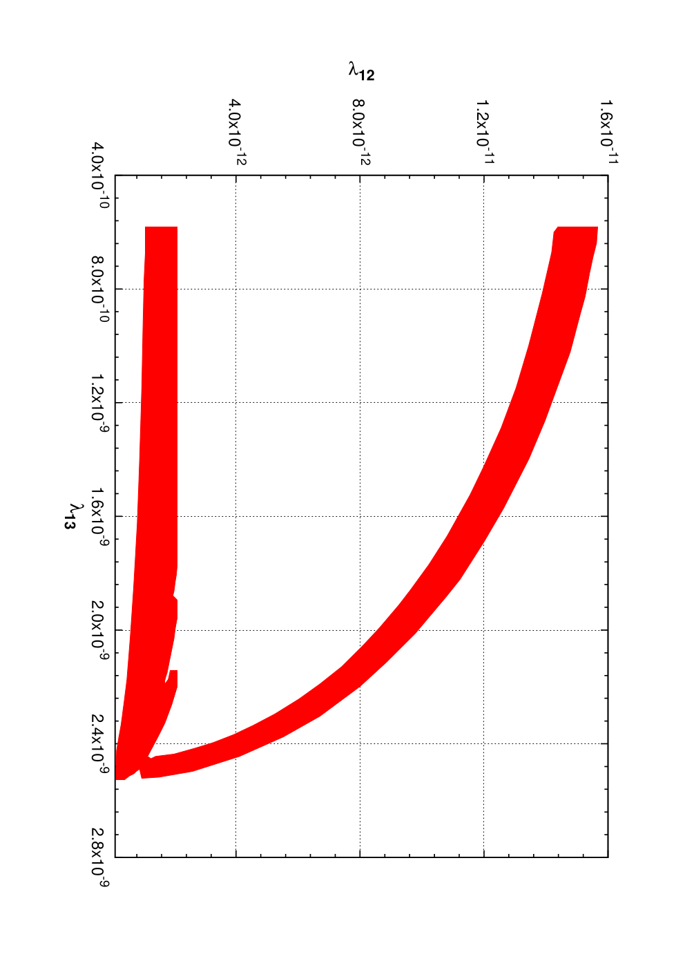
In the three plots (a$-$c) of Fig. 4, we show the allowed regions in the parameter space $\lambda_{12}$-$\lambda_{13}$, $\theta_{12}$-$\theta_{13}$ and $\theta_{12}$-$\theta_{23}$ respectively. These plots (a$-$c of Fig. 4) are drawn for $50\,\,{\rm GeV}\leq M_{\chi_{{}_{{}_{2}}}}\leq 80\,\,{\rm GeV}$, $M_{\chi_{{}_{{}_{3}}}}=7.1$ keV, $2\,\,{\rm MeV}<u\leq 10\,\,{\rm MeV}$, and $10^{-9}\,\,{\rm GeV^{2}}\mathrel{\mathchoice{\vbox{\halign{\hfil$\displaystyle#$\hfil\cr<\cr\sim\cr}}}{\vbox{\halign{\hfil$\textstyle#$\hfil\cr<\cr\sim\cr}}}{\vbox{\halign{\hfil$\scriptstyle#$\hfil\cr<\cr\sim\cr}}}{\vbox{\halign{\hfil$\scriptscriptstyle#$\hfil\cr<\cr\sim\cr}}}}\alpha\mathrel{\mathchoice{\vbox{\halign{\hfil$\displaystyle#$\hfil\cr<\cr\sim\cr}}}{\vbox{\halign{\hfil$\textstyle#$\hfil\cr<\cr\sim\cr}}}{\vbox{\halign{\hfil$\scriptstyle#$\hfil\cr<\cr\sim\cr}}}{\vbox{\halign{\hfil$\scriptscriptstyle#$\hfil\cr<\cr\sim\cr}}}}10^{-7}\,\,{\rm GeV^{2}}$. The choice of the numerical ranges of these parameters will be justified in Sections 4, 6 and 7. In order to avoid the late time decay of the heavier dark matter particle $\chi_{{}_{{}_{2}}}$ into two lighter DM component $\chi_{{}_{{}_{3}}}$, we adopt the value of the parameter $\lambda_{23}\leq 10^{-6}$. The constraint for all the plots of Fig. 4 is that the calculations of relic densities with the allowed values of the parameters must satisfy the PLANCK result for the total relic density of dark matter in the Universe. It is also to be noted that, for plot (a) in Fig. 4, we obtain two allowed regions in the parameter space $\lambda_{12}$-$\lambda_{13}$. The nonthermal production of the present dark matter candidates proceeds through two processes, namely the decay of the SM Higgs and pair annihilation of SM particles. But, if the mass of the heavier dark matter is higher than $M_{\chi_{{}_{{}_{1}}}}/2$, then it will not be produced through the decay of the SM Higgs boson. In this case the heavier dark matter can only be produced by the pair annihilation of SM particles. The lower allowed region in plot (a) between $\lambda_{12}$ and $\lambda_{13}$ is for the case when the mass of the heavier dark matter is less than $M_{\chi_{{}_{{}_{1}}}}/2$ while the other region is for the case when the nonthermal production of the same is through the pair annihilation of SM particles. Needless to mention here that the lighter component can always be produced from the decay of the SM Higgs boson.

References

- [1] G. Bertone, D. Hooper and J. Silk, Phys. Rept. 405, 279 (2005) [hep-ph/0404175].
- [2] P. A. R. Ade et al. [Planck Collaboration], Astron. Astrophys. 571, A16 (2014) [arXiv:1303.5076 [astro-ph.CO]].
- [3] E. Bulbul, M. Markevitch, A. Foster, R. K. Smith, M. Loewenstein and S. W. Randall, Astrophys. J. 789, 13 (2014) [arXiv:1402.2301 [astro-ph.CO]].
- [4] A. Boyarsky, O. Ruchayskiy, D. Iakubovskyi and J. Franse, Phys. Rev. Lett. 113, 251301 (2014) [arXiv:1402.4119 [astro-ph.CO]].
- [5] L. Goodenough and D. Hooper, arXiv:0910.2998 [hep-ph].
- [6] D. Hooper and L. Goodenough, Phys.Lett. B697 (2011) 412–428, arXiv:1010.2752 [hep-ph].
- [7] A. Boyarsky, D. Malyshev, and O. Ruchayskiy, Phys.Lett. B705 (2011) 165–169, arXiv:1012.5839 [hep-ph].
- [8] D. Hooper and T. Linden, Phys.Rev. D84 (2011) 123005, arXiv:1110.0006 [astro-ph.HE].
- [9] K. N. Abazajian and M. Kaplinghat, Phys.Rev. D86 (2012) 083511, arXiv:1207.6047 [astro-ph.HE].
- [10] D. Hooper and T. R. Slatyer, Phys.Dark Univ. 2 (2013) 118–138, arXiv:1302.6589 [astro-ph.HE].
- [11] K. N. Abazajian, N. Canac, S. Horiuchi, and M. Kaplinghat, Phys.Rev. D90 (2014) 023526, arXiv:1402.4090 [astro-ph.HE].
- [12] T. Daylan, D. P. Finkbeiner, D. Hooper, T. Linden, S. K. N. Portillo, et al., arXiv:1402.6703 [astro-ph.HE].
- [13] P. Agrawal, B. Batell, P. J. Fox and R. Harnik, arXiv:1411.2592 [hep-ph].
- [14] F. Calore, I. Cholis, C. McCabe and C. Weniger, arXiv:1411.4647 [hep-ph].
- [15] T. E. Jeltema and S. Profumo, arXiv:1408.1699 [astro-ph.HE].
- [16] E. Carlson, T. Jeltema and S. Profumo, JCAP 1502, no. 02, 009 (2015) [arXiv:1411.1758 [astro-ph.HE]].
- [17] D. Malyshev, A. Neronov and D. Eckert, Phys. Rev. D 90, no. 10, 103506 (2014) [arXiv:1408.3531 [astro-ph.HE]].
- [18] M. E. Anderson, E. Churazov and J. N. Bregman, arXiv:1408.4115 [astro-ph.HE].
- [19] J. Petrovic, P. D. Serpico and G. Zaharijas, JCAP 1410, no. 10, 052 (2014) [arXiv:1405.7928 [astro-ph.HE]].
- [20] J. Petrović, P. D. Serpico and G. Zaharijas, JCAP 1502, no. 02, 023 (2015) [arXiv:1411.2980 [astro-ph.HE]].
- [21] M. S. Boucenna and S. Profumo, Phys. Rev. D 84, 055011 (2011) [arXiv:1106.3368 [hep-ph]].
- [22] J. D. Ruiz-Alvarez, C. A. de S.Pires, F. S. Queiroz, D. Restrepo and P. S. Rodrigues da Silva, Phys. Rev. D 86, 075011 (2012) [arXiv:1206.5779 [hep-ph]].
- [23] A. Alves, S. Profumo, F. S. Queiroz and W. Shepherd, Phys. Rev. D 90, no. 11, 115003 (2014) [arXiv:1403.5027 [hep-ph]].
- [24] A. Berlin, D. Hooper and S. D. McDermott, Phys. Rev. D 89, 115022 (2014) [arXiv:1404.0022 [hep-ph]].
- [25] P. Agrawal, B. Batell, D. Hooper and T. Lin, Phys. Rev. D 90, 063512 (2014) [arXiv:1404.1373 [hep-ph]].
- [26] E. Izaguirre, G. Krnjaic and B. Shuve, Phys. Rev. D 90, 055002 (2014) [arXiv:1404.2018 [hep-ph]].
- [27] D. G. Cerdeño, M. Peiró and S. Robles, JCAP 1408, 005 (2014) [arXiv:1404.2572 [hep-ph]].
- [28] S. Ipek, D. McKeen and A. E. Nelson, Phys. Rev. D 90, 055021 (2014) [arXiv:1404.3716 [hep-ph]].
- [29] C. Boehm, M. J. Dolan and C. McCabe, Phys. Rev. D 90, 023531 (2014) [arXiv:1404.4977 [hep-ph]].
- [30] P. Ko, W. I. Park and Y. Tang, JCAP 1409, 013 (2014) [arXiv:1404.5257 [hep-ph]].
- [31] M. Abdullah, A. DiFranzo, A. Rajaraman, T. M. P. Tait, P. Tanedo and A. M. Wijangco, Phys. Rev. D 90, no. 3, 035004 (2014) [arXiv:1404.6528 [hep-ph]].
- [32] D. K. Ghosh, S. Mondal and I. Saha, arXiv:1405.0206 [hep-ph].
- [33] A. Martin, J. Shelton and J. Unwin, Phys. Rev. D 90, no. 10, 103513 (2014) [arXiv:1405.0272 [hep-ph]].
- [34] L. Wang, arXiv:1406.3598 [hep-ph].
- [35] T. Basak and T. Mondal, arXiv:1405.4877 [hep-ph].
- [36] W. Detmold, M. McCullough and A. Pochinsky, Phys. Rev. D 90, 115013 (2014) [arXiv:1406.2276 [hep-ph]].
- [37] C. Arina, E. Del Nobile and P. Panci, arXiv:1406.5542 [hep-ph].
- [38] N. Okada and O. Seto, Phys. Rev. D 90, no. 8, 083523 (2014) [arXiv:1408.2583 [hep-ph]].
- [39] K. Ghorbani, arXiv:1408.4929 [hep-ph].
- [40] A. D. Banik and D. Majumdar, arXiv:1408.5795 [hep-ph].
- [41] A. Biswas, arXiv:1412.1663 [hep-ph].
- [42] K. Ghorbani and H. Ghorbani, arXiv:1501.00206 [hep-ph].
- [43] D. G. Cerdeno, M. Peiro and S. Robles, arXiv:1501.01296 [hep-ph].
- [44] R. Krall, M. Reece and T. Roxlo, JCAP 1409, 007 (2014) [arXiv:1403.1240 [hep-ph]].
- [45] J. C. Park, S. C. Park and K. Kong, Phys. Lett. B 733, 217 (2014) [arXiv:1403.1536 [hep-ph]].
- [46] M. T. Frandsen, F. Sannino, I. M. Shoemaker and O. Svendsen, JCAP 1405, 033 (2014) [arXiv:1403.1570 [hep-ph]].
- [47] S. Baek and H. Okada, arXiv:1403.1710 [hep-ph].
- [48] K. Nakayama, F. Takahashi and T. T. Yanagida, Phys. Lett. B 735, 338 (2014) [arXiv:1403.1733 [hep-ph]].
- [49] K. Y. Choi and O. Seto, Phys. Lett. B 735, 92 (2014) [arXiv:1403.1782 [hep-ph]].
- [50] M. Cicoli, J. P. Conlon, M. C. D. Marsh and M. Rummel, Phys. Rev. D 90, no. 2, 023540 (2014) [arXiv:1403.2370 [hep-ph]].
- [51] C. Kolda and J. Unwin, Phys. Rev. D 90, 023535 (2014) [arXiv:1403.5580 [hep-ph]].
- [52] R. Allahverdi, B. Dutta and Y. Gao, Phys. Rev. D 89, 127305 (2014) [arXiv:1403.5717 [hep-ph]].
- [53] N.-E. Bomark and L. Roszkowski, Phys. Rev. D 90, no. 1, 011701 (2014) [arXiv:1403.6503 [hep-ph]].
- [54] S. P. Liew, JCAP 1405, 044 (2014) [arXiv:1403.6621 [hep-ph]].
- [55] K. Nakayama, F. Takahashi and T. T. Yanagida, Phys. Lett. B 734, 178 (2014) [arXiv:1403.7390 [hep-ph]].
- [56] E. Dudas, L. Heurtier and Y. Mambrini, Phys. Rev. D 90, 035002 (2014) [arXiv:1404.1927 [hep-ph]].
- [57] K. S. Babu and R. N. Mohapatra, Phys. Rev. D 89, 115011 (2014) [arXiv:1404.2220 [hep-ph]].
- [58] K. P. Modak, arXiv:1404.3676 [hep-ph].
- [59] S. Baek, P. Ko and W. I. Park, arXiv:1405.3730 [hep-ph].
- [60] S. Chakraborty, D. K. Ghosh and S. Roy, JHEP 1410, 146 (2014) [arXiv:1405.6967 [hep-ph]].
- [61] C. W. Chiang and T. Yamada, JHEP 1409, 006 (2014) [arXiv:1407.0460 [hep-ph]].
- [62] B. Dutta, I. Gogoladze, R. Khalid and Q. Shafi, JHEP 1411, 018 (2014) [arXiv:1407.0863 [hep-ph]].
- [63] N. Haba, H. Ishida and R. Takahashi, arXiv:1407.6827 [hep-ph].
- [64] J. M. Cline and A. R. Frey, JCAP 1410, no. 10, 013 (2014) [arXiv:1408.0233 [hep-ph]].
- [65] Y. Farzan and A. R. Akbarieh, JCAP 1411, no. 11, 015 (2014) [arXiv:1408.2950 [hep-ph]].
- [66] T. Higaki, N. Kitajima and F. Takahashi, arXiv:1408.3936 [hep-ph].
- [67] S. Patra, N. Sahoo and N. Sahu, arXiv:1412.4253 [hep-ph].
- [68] K. S. Babu, S. Chakdar and R. N. Mohapatra, arXiv:1412.7745 [hep-ph].
- [69] K. Cheung, W. C. Huang and Y. L. S. Tsai, arXiv:1411.2619 [hep-ph].
- [70] Q. H. Cao, E. Ma, J. Wudka and C.-P. Yuan, arXiv:0711.3881 [hep-ph].
- [71] D. Feldman, Z. Liu, P. Nath and G. Peim, Phys. Rev. D 81, 095017 (2010) [arXiv:1004.0649 [hep-ph]].
- [72] A. Biswas, D. Majumdar, A. Sil and P. Bhattacharjee, JCAP 1312, 049 (2013) [arXiv:1301.3668 [hep-ph]].
- [73] S. Bhattacharya, A. Drozd, B. Grzadkowski and J. Wudka, JHEP 1310, 158 (2013) [arXiv:1309.2986 [hep-ph]].
- [74] L. Bian, T. Li, J. Shu and X. C. Wang, arXiv:1412.5443 [hep-ph].
- [75] J. F. Navarro, C. S. Frenk and S. D. M. White, Astrophys. J. 490, 493 (1997) [astro-ph/9611107].
- [76] E. Aprile et al. [XENON100 Collaboration], Phys. Rev. Lett. 109, 181301 (2012) [arXiv:1207.5988 [astro-ph.CO]].
- [77] D. S. Akerib et al. [LUX Collaboration], Phys. Rev. Lett. 112, no. 9, 091303 (2014) [arXiv:1310.8214 [astro-ph.CO]].
- [78] K. Kannike, Eur. Phys. J. C 72, 2093 (2012) [arXiv:1205.3781 [hep-ph]].
- [79] J. Edsjo and P. Gondolo, Phys. Rev. D 56, 1879 (1997) [hep-ph/9704361].
- [80] A. Biswas and D. Majumdar, Pramana 80, 539 (2013) [arXiv:1102.3024 [hep-ph]].
- [81] L. Dolan and R. Jackiw, Phys. Rev. D 9, 3320 (1974).
- [82] R. Barbieri, L. J. Hall and V. S. Rychkov, Phys. Rev. D 74, 015007 (2006) [hep-ph/0603188].
- [83] M. Cirelli, G. Corcella, A. Hektor, G. Hutsi, M. Kadastik, P. Panci, M. Raidal and F. Sala et al., JCAP 1103, 051 (2011) [Erratum-ibid. 1210, E01 (2012)] [arXiv:1012.4515 [hep-ph], arXiv:1012.4515 [hep-ph]].