The enzyme cost of given metabolic flux distributions, as a function of logarithmic metabolite levels, is convex
Abstract
Enzyme costs play a major role in the choice of metabolic routes, both in evolution and bioengineering. Given desired fluxes, necessary enzyme levels can be estimated based on known rate laws and on a principle of minimal enzyme cost. With logarithmic metabolite levels as free variables, enzyme cost functions and constraints in optimality and sampling problems can be handled easily. The set of feasible metabolite profiles forms a polytope in log-concentration space, whose points represent all possible steady states of a kinetic model. We show that enzyme cost is a convex function on this polytope. This makes enzyme cost minimization – finding optimal enzyme profiles and corresponding metabolite profiles that realize a desired flux at a minimal cost – a convex optimization problem.
1 Introduction
The metabolic fluxes in cells are driven by enzymes, which come at a cost. Translating a given flux profile into the necessary enzyme profile, and computing the corresponding enzyme cost, is not a trivial task. In kinetic models, a reaction rates is a product of enzyme level and an enzyme-specific rate given by the rate law . If metabolite levels were known, the enzyme demand could be directly computed; the specific enzyme demand is simply obtained by inverting the rate law. However, since metabolite levels are not fixed, the fluxes in a network can be realized by many possible enzyme profiles, each with a corresponding metabolite profile. To select a plausible solution, we employ an optimality principle: we define an enzyme cost function (for instance, total enzyme mass) and choose among all possible enzyme profiles the one with the lowest cost. As a constraint, the corresponding metabolite profile must respect physiological ranges and energetic constraints implied by flux directions. The enzyme demand in a reaction, at a given desired flux, depends on thermodynamic and kinetic factors. To see what each factor contributes, we split the formula for enzyme demands into a product of terms, each with a simple interpretation. The reaction rate depends on enzyme level, forward catalytic constant (i.e., the maximal possible forward rate per mM of enzyme), driving force (which determines the relative backward flux), and kinetic effects (such as substrate saturation or allosteric regulation) that modify the forward flux (see Figure 1).

2 Enzymatic rate laws
Reactions of the form A B can be described by the reversible Michaelis-Menten kinetics. A generalized form for reactions with multiple substrates (concentrations ) and products (concentrations ) reads
| (1) |
The molecularities and represent the (positive) stoichiometric coefficients, but they may be scaled by a reaction-specific factor which effectively acts like a Hill coefficient. Using a stoichiometric coefficient and a molecularity is equivalent to using a Hill coefficient of 2 in the rate law. For reasons of thermodynamic consistency, reaction rates must vanish in chemical equilibrium states; to ensure this, equilibrium constants and rate constants must satisfy the Haldane relationship [1]
| (2) |
where and denote to substrate and product levels, respectively. Since the equilibrium constants depend on the Gibbs energies of formation as , they must satisfy Wegscheider conditions [2]: the vector of equilibrium constants satisfies , with the stoichiometric matrix for all metabolites and the vector of transformed Gibbs free energies of formation. Accordingly, the equilibrium constants must satisfy a Wegscheider condition for any thermodynamic cycle , i.e., any nullspace vector of . The denominator in Eq. (1) depends on the enzyme mechanism. In general, it is a polynomial
| (3) |
of the metabolite concentrations with positive coefficients and exponents . For examples of such denominators, see appendix A. In the underlying enzyme mechanism, each sum term (index ) represents a binding state of the enzyme. The exponents indicate the numbers of reactant molecules bound in one binding state and the prefactors encode the binding energies. The sum term 1 represents the unbound enzyme. The highest-order substrate term reads and the highest-order product term reads . In addition, the denominator may contain additive or multiplicative terms for allosteric activation and inhibition. The exponents are usually positive integer numbers. With allosteric regulation, however, there can also be denominator terms of the form .
3 Separable rate laws and enzyme cost
Following [3], we consider general reversible rate laws and factorize them into
| (4) |
where is the forward catalytic constant. For an example of such a factorization, see appendix B. The energetic efficiency
| (5) |
depends on the mass-action ratio (e.g., for unimolecular reactions) and on the equilibrium constant , or briefly on the driving force . Note that our driving forces are defined via molecularities, not via the stoichiometric coefficients; to allow for a consistent equilibrium state, all reactants within a reaction must show the same Hill coefficient [4]. The relationship links concentrations to driving forces and holds for ideal chemical mixtures with constant activity coefficients. The kinetic efficiency depends on the rate law and can be derived from the rate law’s denominator. For a general reversible rate law, the kinetic efficiency would read
| (6) |
where the substrate-dependent numerator stems from the positive numerator term in the rate law and the denominator is given by the rate law denominator. A factorized formula (4), called separable rate law [3], exists for reactions of arbitrary stoichiometry (for examples, see SI A). The factorization is always possible even for general rate laws, because rate law numerators must have the form for reasons of thermodynamic consistency.
(a) Reversible Michaelis-Menten kinetics (factorized, with driving force ) Rate = Enzyme level Forward catalytic constant Energetic efficiency Kinetic efficiency (b) Enzyme cost function (factorized form)
The terms in the rate law (4) depend on metabolite levels in different ways. The first terms, , represent the maximal velocity (the rate at full substrate-saturation, no backward flux, full allosteric activation), while the following efficiency terms describe how this velocity is reduced in reality: the factor describes a reduction due to backward fluxes, and the factors and describe a further reduction due to incomplete substrate saturation and allosteric regulation. While is an enzyme-specific constant (yet, dependent on conditions such as pH, ionic strength, or molecular crowding in cells; unit 1/s), the efficiency terms are concentration-dependent, unitless, and can vary between 0 and 1. The thermodynamic efficiency depends on the driving force (and thus, indirectly, on metabolite levels) and the equilibrium constant is required for its calculation. The kinetic efficiency depends directly on metabolite levels and contains the values as parameters. Allosteric regulation can be captured by (as additive or multiplicative terms in the denominator), but non-competitive allosteric regulation can also be described by a separate term . If rate law, flux, and metabolite levels are known, a reaction’s enzyme demand follows from Eq. (4) as
| (7) |
By weighting the enzyme demand with an enzyme-specific cost , we obtain the cost function
| (8) |
Dividing Eq. (8) by , we obtain the specific flux cost . Eq. (8) shows which factors shape enzyme cost, and how. The first two terms yield the minimal cost (the cost per flux under ideal conditions); the following terms further increase this value. To keep enzyme cost low, the values, driving forces (i.e. imbalance in substrate and product levels), and substrate saturation (i.e. high substrate concentrations) should be high. For a pathway with desired fluxes and known log-concentrations , the total cost reads
| (9) |
Setting , we obtain the total enzyme demand (as a concentration in mM), and setting (protein mass in Daltons), we obtain the mass concentration (in gram protein per cell dry weight) as a special case.
| (a) |
 |
| (b) | (c) | (d) | (e) |
|---|---|---|---|
 |
 |
 |
 |
 |
 |
 |
 |
4 The metabolite polytope represents the states of a kinetic model
A metabolic network (with given flux directions, equilibrium constants, and metabolite bounds) defines a convex metabolite polytope in the space of log-concentrations (where is measured in units of the standard concentration mM). An example is shown in Figure 3. In general, the polytope arises from two sorts of inequality constraints: (i) Upper and lower bounds for metabolite levels yield a box-shaped metabolite polytope; some metabolite levels may also be constrained to a fixed value. (ii) Reaction fluxes dissipate Gibbs energy (), so the driving forces must be positive in the direction of the flux. The resulting constraints further restrict the metabolite polytope; they define E-faces of the polytope (representing an equilibrium condition), where enzyme costs rise steeply. The metabolite polytope is a convex polytope in log-concentration space, which contains all feasible metabolite profiles. It is bounded by two types of faces: faces that represent an equilibrium in one of the reactions (“E-face”), where enzyme cost goes to infinity; and faces stemming from physiological metabolite bounds (“P-face”). Minimum points of the enzyme cost function can be inside the polytope or on P-faces. The polytope’s precise shape depends on the Enzyme Cost Function (ECF) score chosen (i.e, on the simplifications applied) and on rate laws, rate constants, and specific enzyme costs in the model.
The metabolite polytope plays a central role in enzyme cost minimization: For a given model and flux profile , the points of the polytope parametrize the set of all possible steady states . Feasible metabolite profiles (represented by polytope points) can be uniquely mapped to enzyme profiles, while the mapping from enzyme to metabolite profiles need not be unique. The entirety of metabolic states (or all steady states) of a kinetic model can be parametrized as follows: we consider the (non-convex) flux polytope and construct, for each point, the metabolite polytope. The construction yields all steady states (characterized by concentrations, fluxes, enzyme levels) exactly once (while the same enzyme profile may appear several times). Using this fact, we can parametrize all metabolites states of a kinetic model in a simple and systematic way (for details, see appendix C). However, a restriction to stable steady states is not easily possible.
5 Enzyme cost is a convex function on the metabolite polytope
The enzyme cost functions (8) and (9) are differentiable convex functions on the metabolite polytope (proof in SI D). Convexity means that an interpolated metabolite vector, on a line between two log-concentration vectors and , has a cost that is higher than (or at most equal to) the interpolated cost:
| (10) |
To show that the ECF scores are convex, we consider the most general rate laws with denominator (3) and rewrite it in the form
| (11) |
implying the enzyme cost function
| (12) |
for a pathway. The efficiency terms are given by
| (13) |
with coefficients and . The regulation efficiency can be neglected because it can always be covered by the term . The cost function (12) with efficiency terms (13) is convex on the metabolite polytope. The function stays convex if the investment function is not linear, but convex. Importantly, even though all ECF scores are convex, they may not be strictly convex (in which case there would be a sign, instead of , in Eq. (10)). For instance, simplified ECF scores can be constant in the metabolite polytope. Non-strict convexity can arise when the mapping from enzyme to metabolite profiles is not unique. However, it is possible to enforce a unique optimum by adding a convex regularization term , e.g., a quadratic function favoring metabolite levels in the center of the typical concentration range. Such terms can be justified by biological side objectives: for instance, keeping metabolite levels away from their upper or lower bounds in advance will later allow cells to vary them more flexibly. We can also consider a variant of ECM with an additional metabolite-dependent objective . Instead of minimizing the enzyme cost alone, we then minimize the difference . For instance, an objective would represent a preference for metabolite levels close to “ideal” levels , with cost weights . If is strictly concave, can be used as a regularization term . The resulting effective cost will be strictly convex even if the term is very small.
The convexity proof suggests that enzyme levels can be predicted with relatively little effort. Enzyme cost minimization uses a metabolic network, a given flux profile , and possibly kinetic rate laws (with their thermodynamic or kinetic constants), and specific enzyme costs. The flux profile may be stationary (like flux profiles determined by FBA) or non-stationary (like experimentally measured fluxes, simply inserted into a model). In any case, it must be free of thermodynamically unfeasible cycles, and must agree with the assumed equilibrium constants and external metabolite levels. If the given flux directions are infeasible, the metabolite polytope will be an empty set. To find an optimal state, we choose an ECF score and minimize the total enzyme cost within the polytope. Optimal metabolite profiles, enzyme profiles, and enzyme costs are obtained by solving the Enzyme Cost Minimization (ECM) problem
| (14) |
for log-concentration vectors . The total cost (see Eq. (9)) is a sum of enzyme costs (8) or simplified ECF scores. If there is no unique optimum for (because the cost function is constant along some subspace, and therefore not structly convex), a unique solution can be enforced by adding a convex regularization term to . Since the optimal enzyme levels depend on external metabolite levels, they must be recalculated after changes in external conditions. If non-enzymatic reactions (typically with mass-action rate laws) are included in the optimality problem, they contribute to the energetic constraints, but not to the enzyme cost function.
6 Discussion
In summary, we saw that logarithmic metabolite levels are suitable variables for screening, sampling, and optimizion of metabolic states. Due to the mapping from metabolite profiles to enzyme profiles, all feasible enzyme profiles can be reached, where bounds on driving forces can be formulated as linear constraints. Moreover, using the metabolite log-concentrations as free variables does not only provide a good search space, but also facilitates the optimization problem: under general and reasonable assumptions, the ECF scores are convex functions on the metabolite polytope. Convexity holds for a wide range of rate laws, including rate laws with allosteric regulation. As a consequence, the optimization remains tractable for various rate laws and larger metabolic networks. Strict convexity (required for an isolated optimum point) can be enforced by adding small regularization terms , possibly representing biological side objectives.
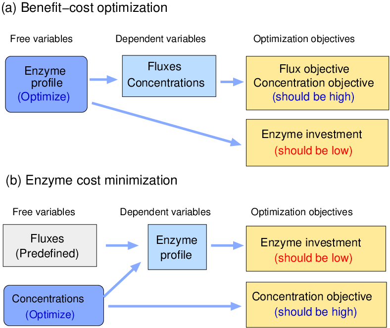
Optimal enzyme allocation in kinetic models can be framed in two main ways. One the one hand, enzyme levels can be treated as control variables which determine the metabolic state, and thus the fluxes (see, e.g., [5, 6]). The aim is to find the enzyme profile that leads to an optimal state (where enzyme cost can come into play as a constraint or as a penalty functions). On the other hand (as in [7, 8] and here), one can predefine the fluxes and search for enzyme levels that realize them in an optimal way (here, minimal cost is used as the optimality criterion). Both approaches address similar problems and lead to equivalent solutions. For instance, if we first maximize a flux at a fixed total enzyme level, as in [6], and then use this flux as a constraint in ECM (with identical specific costs for all enzymes), we recover the metabolite and enzyme profile from the initial calculation. In fact, both optimality problems can be derived from a common general optimality problem by constraining the fluxes or the total enzyme cost. The approaches frame the same problem, but in different ways. Using fluxes as a scaffold for model construction has several advantages. First, it makes the optimality problem convex. Second, we can precisely specify the flux state to be modelled. Third, the flux cost functions can be used in flux analysis. Thus, ECM enables more realistic variants of FBA; the cost function may contain additional side objectives scoring the metabolite levels. If flux profiles are compared at a given flux benefit, it is only the cost scores that count in the optimization, so cost and benefit can be measured in different units. In benefit-cost approaches as in Figure 4 (a), enzyme investment and metabolic objective are directly compared and show the same physical units. In order to make them comparable, a relative weighting would have to be established, which bears the problem of arbitrariness.
Our fundamental assumption – that enzyme levels are cost-optimized in every moment – is of course debatable. Instead, proteins may be expressed to higher amounts to anticipate sudden challenges (example: energy production in muscle cells). Preemptive protein expression can avoid costs for rearranging the proteome and performance losses during adaptation; however, in ECM it would appear futile. Also flexibility in metabolite concentrations can be important, and cells might trade it against enzyme economy. Furthermore, enzyme and metabolite levels in cells are not only shaped by demands in a single pathway, but also by other pathways outside the model in question. Finally, if proteins are used as an amino acid storage, there will be little pressure to keep them at low concentrations. How can our method be useful despite all this? First, an account of simple enzyme economy can be a basis for studying more complicated optimality requirements afterwards. Second, despite all these points of critique, enzyme economy may be the main requirement, e.g., during fast, nitrogen-limited growth. Third, we can study how deviations from the optimal state affect enzyme cost, and thus fitness. Finally, ECM can be extended to include more objectives and constraints into our pathway model, and thus to account for the surrounding cell. The metabolites from our pathway may also be involved in other pathways outside the model. If these other pathways demand higher or lower metabolite levels, we can implement this fact in ECM by constraints (upper and lower concentration bounds) or by concentration-dependent side objectives , which penalize unfavorable metabolite levels. Trade-offs between the pathway in focus and other pathways around it can be handled in this way. Alternatively, we can assume that each metabolite level should be close to the centre of its allowed range (which also provides flexibility, because it will not easily hit a bound). Again, this can be captured by side objectives.
As a possible application, enzyme cost functions allow us to define non-linear flux costs for use in flux balance analysis. ECM is based on a given flux profile. However, since it can be applied to any flux profile, it defines a flux cost function , which can be applied in flux prediction. FBA with minimal fluxes (fmFBA) compares flux profiles at equal benefit (FBA objective) and minimizes their heuristic cost. The flux cost functions used are linear (for a predefined choice of flux directions). Linearity simplifies calculations, but is not very realistic: first, cost scores like the sum of fluxes do not account for kinetics and regulation; second, the costs add linearly when flux distributions are linearly combined. Flux cost functions obtained from ECM, and based on a kinetic model, are more realistic. In an mfFBA based on such cost functions, one would predefine flux directions, flux bounds, and a flux benefit , and assume stationary fluxes; but instead of a linear flux cost, one would minimize the flux cost . Flux costs derived from ECM are concave functions on the flux polytope (with given flux directions). This implies that the solutions of the new fmFBA problems will be elementary flux modes, which confirms findings from other enzyme optimality approaches [9, 10]. In fact, the flux cost function can be expected to be strictly concave (except for specific cases, e.g. models containing two identical reactions with identical rate laws). If this is this case, elementary flux modes are the only solutions. As a consequence, splitting a flux profile into elementary modes that run in different compartments or at different time points can be better, but never worse than the original flux profile in terms of enzyme cost.
Acknowledgements
The authors thank Avi Flamholz, Ron Milo, Frank Bruggeman, Joost Hulshof, and Meike Wortel for inspiring discussions. This work was supported by the German Research Foundation (Ll 1676/2-1).
References
- [1] J.B.S. Haldane. Enzymes. Longmans, Green and Co., London. (republished in 1965 by MIT Press, Cambridge, MA), 1930.
- [2] R. Wegscheider. Über simultane Gleichgewichte und die Beziehungen zwischen Thermodynamik und Reactionskinetik homogener Systeme. Z. Phys. Chem., 39:257–303, 1902.
- [3] E. Noor, A. Flamholz, W. Liebermeister, A. Bar-Even, and R. Milo. A note on the kinetics of enzyme action: a decomposition that highlights thermodynamic effects. FEBS Letters, 587(17):2772–2777, 2013.
- [4] W. Liebermeister, J. Uhlendorf, and E. Klipp. Modular rate laws for enzymatic reactions: thermodynamics, elasticities, and implementation. Bioinformatics, 26(12):1528–1534, 2010.
- [5] J.G. Reich. Zur Ökonomie im Proteinhaushalt der lebenden Zelle. Biomed. Biochim. Acta, 42(7/8):839–848, 1983.
- [6] R. Heinrich and E. Klipp. Control analysis of unbranched enzymatic chains in states of maximal activity. J. Theor. Biol., 182(3):243–252, 1996.
- [7] A. Flamholz, E. Noor, A. Bar-Even, W. Liebermeister, and R. Milo. Glycolytic strategy as a tradeoff between energy yield and protein cost. PNAS, 110(24):10039–10044, 2013.
- [8] N. Tepper, E. Noor, D. Amador-Noguez, H.S. Haraldsdóttir, R. Milo, J. Rabinowitz, W. Liebermeister, and T. Shlomi. Steady-state metabolite concentrations reflect a balance between maximizing enzyme efficiency and minimizing total metabolite load. PLoS ONE, 8(9):e75370, 2013.
- [9] S. Müller, G. Regensburger, and R. Steuer. Enzyme allocation problems in kinetic metabolic networks: Optimal solutions are elementary flux modes. Journal of Theoretical Biology, 347:182–190, 2014.
- [10] M.T. Wortel, H. Peters, J. Hulshof, B. Teusink, and F.J. Bruggeman. Metabolic states with maximal specific rate carry flux through an elementary flux mode. FEBS Journal, 281(6):1547–1555, 2014.
- [11] W. Liebermeister and E. Klipp. Bringing metabolic networks to life: convenience rate law and thermodynamic constraints. Theor. Biol. Med. Mod., 3:41, 2006.
| Name | Symbol | Unit |
|---|---|---|
| Flux | mM/s | |
| Metabolite level | mM | |
| Logarithmic metabolite level | mM | |
| Enzyme level | mM | |
| Reaction rate | mM/s | |
| Specific rate | 1/s | |
| Scaled reactant elasticity | 1 | |
| Gibbs free energy of formation | kJ/mol | |
| Reaction Gibbs energy | kJ/mol | |
| Driving force | 1 | |
| Forward/backward catalytic constant | 1/s | |
| Michaelis-Menten constant | mM | |
| Specific enzyme cost | D/mM | |
| Enzyme cost | D | |
| Total enzyme cost | D | |
| Specific flux cost | D/(mM/s) | |
| Enzyme-optimal cost | D |
Appendix A Kinetic rate laws
By considering simple enzyme mechanisms with few binding states, we obtain general rate laws applicable to all reaction stoichiometries. The rate law denominators to be used in Eq. (1) have simple structures (containing only few of the possible sum terms, and with prefactors following from a few Michaelis-Menten constants) [4]. If denominator terms are omitted, the rate will be overestimated, i.e., enzyme demand and costs will be underestimated. First, there are rate laws with denominators
| (15) |
which lead to the energetics-based ECF2 scores. The big product terms are called principal substrate and product terms. As before, and denote substrate and product levels. The first formula assumes that substrate levels are high and product levels are low; the second one assumes that substrate and product levels are both high. Next, there are rate laws with denominators
| (16) |
which lead to the saturation-based ECF3 scores. The denominators contain only three possible terms: the term 1, the principal substrate term, and the principal product term. To justify these rate laws, we assume a strongly cooperative binding between substrates and between products. The first formula assumes low product concentrations; the second formula describes the direct-binding modular rate law [4]. The direct-binding modular rate law is a generalized version of reversible MM kinetics. In the underlying enzyme mechanism, the enzyme exists in three states: fully bound with substrates, fully bound with products, or empty. If enzymes are allosterically regulated, the rate law denominators contain additive or multiplicative terms for regulation [4]. Additive terms can arise from competitive regulation. Multiplicative terms (for non-competitive regulation) can be split from the denominator and treated as prefactors in the rate law. Typical choices are for non-competitive activation and for non-competitive inhibition, with rate constants and and regulator concentration [4]. Accordingly, allosteric effects can either be listed by a separate efficiency term in the factorized ECF formulae, or be included in the kinetic efficiency. For instance, the kinetic efficiency term for MM-kinetics with non-competitive inhibition can be split into
| (17) |
Appendix B Factorization of rate laws
To demonstrate how rate law are factorized, we consider the common modular rate (CM) law [11, 4], a generalized form of reversible MM kinetics with the denominator
| (18) |
In the assumed enzyme mechanism, substrate molecules bind independently, product molecules bind independently, and substrate and product binding exclude each other. For a bimolecular reaction , the rate law
| (19) |
can be rewritten as
| (20) | |||||
where we defined the kinetic efficiency
| (21) |
and used the Haldane relationship and the identity . In the calculation, we first separated the value from the rest of the fraction, and then hid the negative flux term in the energetic efficiency term .
Appendix C Parametrizing all states of a kinetic model
In a kinetic model with given rate laws and external metabolite concentrations, an enzyme profile lead to a steady state with metabolite levels and fluxes . The following proposition shows how the set of such steady states can be easily parametrized.
Proposition: Consider a kinetic model with rate laws , thermodynamically consistent rate constants (satisfying Wegscheider conditions and Haldane relationships), a feasible positive flux profile , and bounds on metabolite levels. Any feasible metabolite profile can be realized by some positive enzyme profile ; given the metabolite levels, the enzyme levels are uniquely determined and given by , which is a differentiable function on the metabolite polytope.
Proof: If a metabolite profile is feasible for the given flux profile , the specific rates obtained from reveresible rate laws (see Eq. (1) in appendix) have the same signs as , so is positive on the entire metabolite polytope. Since is differentiable and does not change its sign on the metabolite polytope, is differentiable on the metabolite polytope.
According to our proposition, any thermodynamically feasible metabolite profile can be realized by some steady state of the kinetic model (with an appropriate choice of enzyme levels), so the set of metabolic states with a given flux profile can be characterized by points of the metabolite polytope. In particular, the set of kinetically realizable metabolite profiles depends on the equilibrium constants, but not on enzyme-specific rate constants.
With simplified rate laws, the same enzyme profile may be realizable by different metabolite profiles. (i) If a metabolite appears in a model but has no impact on any reaction, its concentration can be freely varied, independently of the enzyme levels. (ii) With simplified cost scores in which all efficiencies , , and are taken to be constant, enzyme levels do not depend on metabolite levels. (iii) With simplified scores in which and are taken to be constant, enzyme costs depend on metabolite levels only through the thermodynamic forces. Notably, the vector can be varied along directions in the nullspace of without affecting the driving forces or enzyme cost. Thus, the enzyme cost scores have an invariant subspace on the metabolite polytope (namely the nullspace of ). Under what conditions more complicated enzyme cost scores (without regularisation terms) have unique optima remains an open question.
Finally, to parametrize all steady states of a kinetic model, we can follow a two-step procedure in which we enumerate all possible flux distributions and, for each of them, all possible enzyme and metabolite profiles. The thermodynamically feasible flux distributions form a set , given by , where stands for log-concentration profiles. The reaction Gibbs energies depend on the internal and external metabolite levels and on the equilibrium constants chosen. According to thermodynamic condition, whether a flux distributions is feasible or infeasible depends solely on its sign pattern. By imposing upper and lower bounds and the stationarity condition, we can further limit this set and obtain the set of feasible, stationary fluxes . is a (generally non-convex) polytope in flux spaces. Each flux distribution in this set defines a set of possible states , one can then set .
Appendix D Convexity proof for enzyme cost functions
To prove the convexity of general enzyme cost functions, on the metabolite polytope and at given desired fluxes, we first show the convexity of some simple functions appearing in the formula.
D.1 General lemmata
Lemma 1
The function is convex in the range .
Proof D.1
The second derivative
is positive for .
Lemma 2
The function is convex.
Proof D.2
since from the Cauchy-Schwarz inequality. Therefore, the Hessian is positive semi-definite, which proves that is convex.
Lemma 3
For any number and vector , the function is convex over
Proof D.3
This function is a composition of from Lemma 1 with the affine transformation , an operation which preserves convexity.
Lemma 4
For any matrix and vectors , the following function is convex over :
| (22) |
where is the th row of .
Proof D.4
This function is a composition of from Lemma 2 with the affine transformation , an operation which preserves convexity.
D.2 The convexity of enzyme cost functions
Lemma 5
Assume that all enzyme-catalysed reactions in a model behave according to rate laws of the type
| (23) |
with and given by Eq. (13), with coefficients and . Assume that the enzyme cost function for enzymatic reaction reads
| (24) |
Then the total enzyme cost , as a function of logarithmic metabolite concentrations (), is convex.
Proof D.5
To simplify the efficiency terms, we can use the abbreviations , , and :
| (25) |
If we look at the natural logarithm of ,
| (26) |
we see that each of the three terms in the sum is convex in . The first term is constant with respect to the metabolite concentrations and therefore trivially convex. The energetic term, , is convex according to Lemma 3. The kinetic term, , is convex according to Lemma 4. We conclude that is convex too, since it is a composition of a convex function () with another convex function (). Finally, the total enzyme cost () is convex since it is a sum of convex functions:
| (27) |