Gap formation and stability in non-isothermal protoplanetary discs

In the energy equation, the heating term $\mathcal{H}$ is defined as

where $Q^{+}$ represents viscous heating (from both physical and artificial viscosity) and subscript $i$ denotes evaluation at $t=0$. The cooling term $\mathcal{C}$ is defined as

where $t_{c}=\beta\Omega_{k}^{-1}$ is the cooling time, $\Omega_{k}=\sqrt{GM/r^{3}}$ is the Keplerian frequency and $\beta$ is an input parameter. This cooling prescription allows one to explore the full range of thermodynamic response of the disc in a systematic way: $\beta\ll 1$ is a locally isothermal disc while $\beta\gg 1$ is an adiabatic disc.

Note that the energy source terms have been chosen to be absent at $t=0$, allowing the disc to be initialized close to steady state. The $\mathcal{C}$ function attempts to restore the initial energy density (and therefore temperature) profile. In practice, this is a cooling term at the gap edge because disc-planet interaction leads to heating.

The disc occupies $r\in[r_{\mathrm{in}},r_{\mathrm{out}}]$ and $\phi\in[0,2\pi]$. The initial disc is axisymmetric with surface density profile

where the power-law index $s=2$, $H(r)=c_{\mathrm{iso}}\Omega_{k}$ defines the disc scale-height where $c_{\mathrm{iso}}=\sqrt{p/\Sigma}$ is the isothermal sound-speed. The disc aspect ratio is defined as $h\equiv H/r$ and initially $h=0.05$. For a non-self-gravitating disc, the surface density scale $\Sigma_{\mathrm{ref}}$ is arbitrary.

The initial azimuthal velocity $v_{\phi i}$ is set by centrifugal balance with pressure forces and stellar gravity. For a thin disc, $v_{\phi}\simeq r\Omega_{k}$. The initial radial velocity is $v_{r}=3\nu/r$, where $\nu=\hat{\nu}r_{\mathrm{in}}^{2}\Omega_{k}(r_{\mathrm{in}})$, and we adopt $\hat{\nu}=10^{-9}$, so that $|v_{r}/v_{\phi}|\ll 1$ and the initial flow is effectively only in the azimuthal direction. With this value of physical viscosity, the only source of heating is through compression, shock-heating (via artificial viscosity) and the $\mathcal{C}$ function when $e/\Sigma<e_{i}/\Sigma_{i}$.

The planet potential is given by

where $M_{p}$ is the planet mass and we fix $q\equiv M_{p}/M_{*}=10^{-3}$ throughout this work. This corresponds to a Jupiter-mass planet if $M_{*}=M_{☉}$. The planet’s position in the disc $\bm{r}_{p}=(r_{p},\phi_{p})$ and $\epsilon_{p}=0.5r_{h}$ is a softening length with $r_{h}=(q/3)^{1/3}r_{p}$ being the Hill radius. The planet is held on a fixed circular orbit with $r_{p}=10r_{\mathrm{in}}$ and $\phi_{p}=\Omega_{k}(r_{p})t$. This also defines the time unit $P_{0}\equiv 2\pi/\Omega_{k}(r_{p})$ used to describe results.

In this work we only vary one control parameter: the cooling time. The cooling parameter $\beta$ is chosen indirectly through the parameter $\tilde{\beta}$ such that

where $x_{s}$ is the distance from the planet to its gap edge, and $t_{\mathrm{lib}}$ is the time interval between successive encounters of a fluid element at the gap edge and the planet’s azimuth. That is, we measure the cooling time in units of the time interval between encounters of a fluid element at the gap edge and the planet-induced shock.

Assuming Keplerian orbital frequencies and $x_{s}\ll r_{p}$ gives $t_{\mathrm{lib}}\simeq 4\pi r_{p}/(3\Omega_{kp}x_{s})$, where $\Omega_{kp}=\Omega_{k}(r_{p})$. Therefore

where $x_{s}\ll r_{p}$ was used again. We use $x_{s}=2r_{h}$ in Eq. 9. For a planet mass with $q=10^{-3}$, Eq. 9 then gives $\beta\simeq 23.9\tilde{\beta}$. In terms of planetary orbital periods, this is

We first compare the gap structures formed by planet-disc interaction as a function of the cooling time. The azimuthally-averaged gap profiles are shown in Fig. 1 for different values of $\tilde{\beta}$. Gaps formed with lower $\tilde{\beta}$ (faster cooling) are deeper with steeper gradients at the gap edges. Faster cooling rates also increase (decrease) the surface density maxima (minima). However, a clean gap does not form in this short time period.

Increasing $\tilde{\beta}$ leads to higher disc aspect ratios $h=H/r$, i.e. higher temperatures. Heating mostly occurs at the gap edges due to planet-induced spiral shocks. Increasing the cooling timescale implies that this heat is retained in the disc. In the inviscid limit the gap opening condition is $r_{h}\;\raisebox{-3.44444pt}{$\mathrel{\mathop{\kern 0.0pt\sim}\limits^{\textstyle>}}$}\;H$ or $q\;\raisebox{-3.44444pt}{$\mathrel{\mathop{\kern 0.0pt\sim}\limits^{\textstyle>}}$}\;3h^{3}$ (Crida, Morbidelli & Masset, 2006), which indicates that for hotter discs (higher $h$), it becomes more difficult for a planet of fixed $q$ to open a gap. This explains the shallower gaps in surface density when $\tilde{\beta}$ is increased.

The important consequence of a heated gap edge is that the generalised vortensity profiles, $\tilde{\eta}$, becomes smoother with increasing cooling times, with the extrema becoming less pronounced. Previous locally isothermal disc-planet simulations show the RWI associated with PV minima (Li et al., 2005; Lin & Papaloizou, 2010). We can therefore expect the RWI to be associated with minima in the generalised vortensity (corresponding to local surface density maxima) in the non-isothermal case. Because the extrema are less sharp, the RWI is expected to be weaker and the gap to be more stable with longer cooling times.

However, we remark that the change in the gap structure becomes less significant at long cooling times, as Fig. 1 shows that the profiles with $\tilde{\beta}=1$ and $\tilde{\beta}=10$ are similar. This implies that the effect of cooling timescale on the RWI through the set up of the gap profile, becomes less important for large $\tilde{\beta}$.

The initial planet-disc interaction form bumps and grooves in the gap profiles which can potentially be unstable due to axisymmetric instabilities. The generalised local axisymmetric stability condition is the Solberg-Hoiland criterion,

where

is the square of the Brunt-Väisälä frequency. At the outer gap edge $r=r_{p}+2.5r_{h}$, where the RWI is excited (see below), we find $\kappa^{2}+N^{2}$ reaches local minimum with a value $\sim 0.45\,\Omega^{2}(r_{p})$ for all $\tilde{\beta}$. The Brunt-Väisälä frequency at the outer gap edge is $N\sim 0.1\,\Omega(r_{p})$, decreasing marginally with longer cooling rate. The Solberg-Hoiland criteria is similarly satisfied for the entire 2D disc throughout the simulations. Thus for all values of $\tilde{\beta}$ the planet-induced gaps are stable to axisymmertic perturbations.

We now examine the evolution of the gap for $t>30P_{0}$, with the planet potential switched off, but with an added surface density perturbation. For all three cooling times $\tilde{\beta}=0.1,\,1.0,\,10$, we observe exponential growth of non-axisymmetric structures. An example is shown in Fig. 2 for $\tilde{\beta}=10$. We characterize these modes with an azimuthal wavenumber $m$ and growth rate $\sigma(m)$ as defined by Eq. 12—13. Mode amplitudes were averaged over $r-r_{p}\in[2,5]r_{h}$. Table 1 lists the growth rates measured during linear growth for 5 values of $m$ centred around that with maximum growth rate.

Table 1 show that as $\tilde{\beta}$ is increased from $0.1\rightarrow 10$ the dominant azimuthal Fourier mode decreases from $m=9\rightarrow 3$ and the respective growth rate decreases from $\gamma/\Omega(r_{p})=0.079\rightarrow 0.017$. However, despite two orders of magnitude increase in the cooling time, the instability remains dynamical with characteristic growth time $\;\raisebox{-3.44444pt}{$\mathrel{\mathop{\kern 0.0pt\sim}\limits^{\textstyle<}}$}\;10P_{0}$. Snapshots of the instability in for the different $\tilde{\beta}$ are shown in Fig 3.

These ‘planet-off’ simulations show that gap edges become more stable with longer cooling times. This is expected because larger $\tilde{\beta}$ results in hotter gap profiles at $t=30P_{0}$ with less pronounced generalised vortensity minima. Stabilization with increased cooling time is therefore due to a smoother basic state for the instability, as it is more difficult for the planet to open a gap if the disc is allowed to heat up.

For completeness we also simulated a locally isothermal disc with $h=0.05$ where the sound-speed is kept strictly equal to its initial value. This simulation yield a most unstable growth rate $\sigma/\Omega(r_{p})\simeq 0.05$ at $m=5$, compared with a value of $0.085$ at $m=6$ for a corresponding simulation that includes the energy equation but with rapid cooling $\tilde{\beta}=0.01$. However, the vortex evolution is similar.

We also extended these ‘planet-off’ simulations into the non-linear regime. After the linear growth phase of the vortices, vortex merging takes hold on timescales of up to $150P_{0}$, until there is one vortex left. We find the vortex merging time is dependent on the growth rates of the modes and saturation timescales, with the slowest growing modes in $\tilde{\beta}=10$ taking the longest to merge.

Fig.4 shows evolution of the $m=1$ surface density component, which represents the amplitude of the post-merger single vortex. For completeness we also ran intermediate cases with $\tilde{\beta}=0.5$ and $5.0$. The amplitude of the initially formed vortex was found to decrease with increased cooling rate. The vortices simply decay on a timescale of $O(10^{3})$ orbits with faster decay for stronger vortices (which are obtained with faster cooling rates).

This decay is probably due to numerical viscosity. During the slow decay the vortex elongates (weakens) while its radial width remains $O(H)$, so its surface density decreases. In addition, for $\tilde{\beta}=0.1,\,0.5$ and $1.0$ we also observe the appearance of spiral waves associated with the vortex, which may contribute to its dissipation (see below). We will see in the next section that this decay after linear growth is very different to when the planet potential is kept on.

The linear growth of the RWI and vortex-formation is followed by vortex merging. We now find merging timescales independent of $\tilde{\beta}$, and by $60P_{o}$ only one vortex remains. The evolution of the amplitude of the $m=1$ surface density component, averaged over $r-r_{p}\in[2,10]r_{h}$, is shown in Fig. 5 for different $\tilde{\beta}$. The initial, post-merger vortex amplitude is found to be weaker for longer cooling rates (which have smaller linear growth rates).

In all cases the system remains in a quasi-steady state for $\;\raisebox{-3.44444pt}{$\mathrel{\mathop{\kern 0.0pt\sim}\limits^{\textstyle>}}$}\;800P_{0}$ with a single vortex circulating the outer gap edge at the local Keplerian frequency. Fig. 6 shows a typical plot of the relative surface density perturbation in this state. During this stage, the vortex intensifies. This is better shown in Fig. 7 as the evolution of Rossby numbers measured at the vortex centres. The Rossby number increases in magnitude during quasi-steady state, but the maximum $|Ro|$ is similar for all $\tilde{\beta}$: the vortex reaches a characteristic value of $Ro\approx-0.35$ for $\tilde{\beta}=0.1$ and $Ro\approx-0.45$ for $\tilde{\beta}=10$.

We find the vortices become significantly over-dense. Fig. 8 plots the surface density perturbation measured at the vortex centres, showing $\Delta\Sigma/\Sigma_{0}\;\raisebox{-3.44444pt}{$\mathrel{\mathop{\kern 0.0pt\sim}\limits^{\textstyle>}}$}\;7$ for all cases of $\tilde{\beta}$ in quasi-steady state, and $\mathrm{max}(\Delta\Sigma/\Sigma_{0})\sim 11$ for $\tilde{\beta}=5$. The maximum over-density typically increases with longer cooling times, despite the vortices are initially weaker at formation with increasing $\tilde{\beta}$. The large increase in the surface density is due to vortex growth as there is continuous generation of vorticity by planet-disc interaction. This is supported by the observation that in the previous simulations without the planet, the amplitude of the post-merger vortex does not grow (Fig. 4).

Fig. 5 shows that the duration of the quasi-steady state varies with the cooling rate: for $\tilde{\beta}=0.1$ and $10$, the vortex amplitude begins to decay around $t\sim 800P_{0}$, while for $\tilde{\beta}=1,\,5$ the decay begins at $t\sim 1200P_{0}$. This non-monotonic dependence suggests that there exists an optimal cooling rate to maximise the vortex lifetime. We will discuss this issue further in §5.4. Notice the decay timescale can be long with rapid cooling: for $\tilde{\beta}=0.1$ it takes $\sim 400P_{0}$ whereas for $\tilde{\beta}=10$ it takes $\sim 100P_{0}$ for the $m=1$ amplitude to decay significantly after reaching maximum.

In this subsection we examine the vortex decay observed in our simulations in more detail. Fig. 9 show snapshots of the vortex for the case $\tilde{\beta}=1$. The plots show the surface density perturbation and the surface density gradient during quasi-steady state ($t=700P_{0}$), when the $m=1$ amplitude begins to decrease ($t=1300P_{0}$) and just after the rapid amplitude decay ($t=1510P_{0}$).

In quasi-steady ($t=700P_{0}$) the vortex is elongated with a vortex aspect ratio $\approx 4$ , but becomes more compact approaching a ratio of 2 during its decay ($t=1310P_{0}$). Notice in Fig. 9 the appearance of wakes extending from either side of the vortex at $t=1300P_{0}$. These wakes correlate with large gradients in surface density (bottom panel), and are first seen in the later half of the quasi-steady state. We find the time at which the vortex begins to decay coincides with the emergence of these wakes.

During the quasi-steady state the vortex orbits at $r\sim r_{p}+6r_{h}$. We do not see significant vortex migration at this stage, since the vortex is located at a surface density maximum (Paardekooper, Lesur & Papaloizou, 2010). However, simultaneous with the appearance of the wakes, we observe the vortex begins to migrate inwards to $r\sim r_{p}+5r_{h}$.

During quasi-steady state the average value of the surface density gradient along the wakes is $|w_{s}\nabla\Sigma/\Sigma|\sim 0.4$, where $w_{s}\simeq 0.1$ (code units) is a typical length scale of the surface density variation across the wake. Just before the $m=1$ amplitude begins to decrease, we observe this quantity sharply increases to $\sim 0.6$, and remains around this value until the vortex dies out, at which point the associated Rossby number begins decreasing to zero. After the vortex reaches small amplitudes ($1\;\raisebox{-3.44444pt}{$\mathrel{\mathop{\kern 0.0pt\sim}\limits^{\textstyle<}}$}\;\Delta\Sigma/\Sigma$), it migrates out to $r\sim r_{p}+6.5r_{h}$.

We also measured large increases in the Mach number near the vortex as the $m=1$ surface density amplitude reaches maximum and begins to decay. Fig. 10 plots the Mach number $M=|\bm{v}-\bm{v}_{\mathrm{vor}}|/c_{s}$, where $\bm{v}_{\mathrm{vor}}$ corresponds to the bulk velocity of the vortex around the disc. Values in Fig. 10 have been averaged over a region within $2H$ of the vortex centre. During the quasi-steady state the Mach number increases steadily, and for all cases $M$ maximizes about $\sim 100P_{0}$ after the start the $m=1$ surface density amplitude starts to decay.

Putting the above observations together, we suggest that vortex decay (in the $m=1$ surface density amplitude) is due to shock formation by the vortex. When the vortex reaches large amplitude, it begins to induce shocks in the surrounding fluid, as supported by the increase in Mach number and the appearance of wakes with large surface density gradients. The vortex may lose energy through shock dissipation. In addition, a strong vortex (or shock formation) can smooth out the gap structure that originally gave rise to the RWI, which would oppose vortex growth. We examine this below.

We find vortex decay modifies the gap structure. Fig. 11 shows the gap profile before and after vortex decay for the case $\tilde{\beta}=1$. The vortex resides around the local surface density maximum at the outer gap edge ($r\sim r_{p}+6r_{h}$). We see that after its amplitude has decayed ($t\sim 1500P_{0}$, Fig. 5), this local surface density maximum is also smoothed out.

We characterize the smoothness of the outer gap edge with a dimensionless gap edge gradient parameter

where $\Delta r=r\in[r_{p},r_{p}+6r_{h}]$ is the radial range of averaging, spanning from centre of the gap to the radius of the surface density maximum. A larger $\delta\Sigma$ characterizes a sharper gap edge and larger local surface density maxima.

A plot of the gradient parameter over time for the $\tilde{\beta}=1.0$ case is shown in Fig. 12. During vortex decay, the outer gap edge is drastically smoothed out, changing from a value of $\delta\Sigma=1.2$ during quasi-steady state to $0.4$ after dissipation.

This can be interpreted as the vortex providing a viscosity; and we measure a typical alpha viscosity $\alpha=O(10^{-2})$ associated with the vortex. This acts against gap-opening by the planet, and smooths out the outer surface density bump, so the condition for the RWI becomes less favourable. In order to re-launch the RWI, the surface density bump should reform. However, this is difficult as there is no more material in the planet’s vicinity to clear out (Fig. 11) to form a surface density bump outside the gap. This may explain why vortices do not reform again (at least within the simulation timescale). After full decay the aspect ratio at the outer gap edge is $h\sim 0.05$.

We now examine vortex lifetimes as function of the imposed cooling times. For this study, additional simulations with $\tilde{\beta}=0.01,\,0.25,\,0.75,\,2.5,\,7.5$ were also performed. We define the vortex lifetime, $t_{\mathrm{life}}$, as the time at which the over-density of the vortex returns to $\Delta\Sigma/\Sigma_{0}\sim 1$ after reaching maximum (which is on the order of the initial over-density associated with the gap formation).

We plot $t_{\mathrm{life}}$ with respect to cooling times in Fig. 13. We also plot $t_{\mathrm{diss}}$: the time elapsed before the vortex to begins to dissipate (when the $m=1$ surface density amplitude begins to decay); and $t_{\mathrm{Mach}}$: the time taken for the average Mach number around the vortex to maximise.

For fast cooling rates ($\tilde{\beta}\;\raisebox{-3.44444pt}{$\mathrel{\mathop{\kern 0.0pt\sim}\limits^{\textstyle<}}$}\;1$), the vortex lifetime is maximized for $\tilde{\beta}\to 0$: we find $t_{\mathrm{life}}\approx 2100P_{0}$ for $\tilde{\beta}=0.01$ and decreases to $t_{\mathrm{life}}\approx 950P_{0}$ for $\tilde{\beta}=0.25$. Note that for very small $\tilde{\beta}$, there is significant contribution to the overall vortex lifetime due to a long decay timescale. For longer cooling times ($\tilde{\beta}\;\raisebox{-3.44444pt}{$\mathrel{\mathop{\kern 0.0pt\sim}\limits^{\textstyle>}}$}\;1$) the vortex lifetimes maximizes at $\tilde{\beta}=2.5$ with $t_{\mathrm{life}}\approx 1650P_{0}$.

We comment here that a locally isothermal simulation, where the disc sound-speed is kept constant in time, was also performed for comparison. In this case we did not observe significant vortex decay within the simulation timescale (implying $t_{\mathrm{diss}}\;\raisebox{-3.44444pt}{$\mathrel{\mathop{\kern 0.0pt\sim}\limits^{\textstyle>}}$}\;2000P_{0}$). We expect the corresponding vortex lifetime to exceed that for $\tilde{\beta}=0.01$. Including an energy equation with rapid cooling (or setting $\gamma$ close to unity), could still lead to discrepancies with a locally isothermal disc. This is due to the advection-creation of specific entropy within the planet’s horseshoe region with the former case, thereby affecting the generalized vortensity and therefore the instability (§4.3) and subsequent vortex evolution. Nevertheless, a longer vortex lifetime in a locally isothermal disc would be consistent with the above trend of increasing vortex lifetimes as $\tilde{\beta}\to 0$.

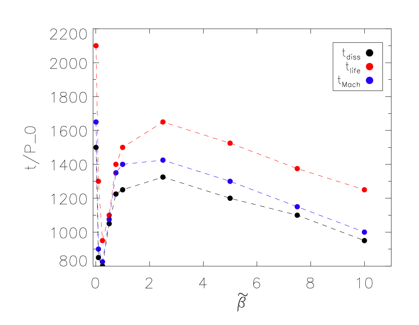
In the previous section, we observed that vortices began to decay when it starts to induce shocks. We thus suggest that the time needed for the vortex to grow to sufficient amplitude to induce shocks in the surrounding fluid, which may be considered as the duration of the quasi-steady state or $t_{\mathrm{diss}}$, is an important contribution to the overall vortex lifetime. We discuss below some competing factors that may result in a non-monotonic dependence of $t_{\mathrm{diss}}$ on the cooling rate.

There are several outstanding issues that needs to be addressed in future work:

Convergence. Although lower resolution simulations performed in the early stages of this project gave similar results (most importantly, the non-monotonic dependence of vortex lifetimes on the cooling timescale), we did find the lower resolution typically yield longer vortex lifetimes than that reported in this paper. This could be due to weaker RWI with low resolution. It will be necessary to perform even higher resolution simulations in order to obtain quantitatively converged vortex lifetimes.

Orbital migration. We have held the planet fixed on a circular orbit. However, gap-edge vortices are known to exert significant, oscillatory torques on the planet (Li et al., 2009) which can lead to complex orbital migration. This will likely affect vortex lifetimes as it may alter the planet-vortex separation, as well as leading to direct vortex-planet interactions (Lin & Papaloizou, 2010; Ataiee et al., 2014). Thus, future simulations should allow the planet to freely migrate. Similarly, the role of vortex migration on its lifetime should be clarified.

Cooling model. Our prescription for the disc heating/cooling is convenient to probe the full range of thermodynamic response of the disc. However, in order to calculate vortex lifetimes in actual protoplanetary discs, an improved thermodynamics treatment, e.g. radiative cooling based on realistic disc temperature, density, opacity models etc., should be used in future work.

Self-gravity. We have ignored disc self-gravity in this study. Based on linear calculations, Lovelace & Hohlfeld (2013) concluded self-gravity to be important for the RWI when the Toomre parameter $Q<O(1/h)$, or $Q\;\raisebox{-3.44444pt}{$\mathrel{\mathop{\kern 0.0pt\sim}\limits^{\textstyle<}}$}\;20$ for $h\sim 0.05$, as was typically considered in this work. This suggests that self-gravity may affect vortex lifetimes even when $Q$ is not small. In particular, given that we observe vortices can reach significant over-densities (up to almost an order of magnitude), it will be important to include disc self-gravity in the future.

Three-dimensional (3D) effects. A vortex in a 3D disc may be subject to secondary instabilities that destroy them (Lesur & Papaloizou, 2009; Railton & Papaloizou, 2014). This may be an important factor in determining gap-edge vortex lifetimes in realistic discs. For example, if these secondary instabilities sets in before the vortex grows to sufficient amplitude to shock, then the dependence of the vortex lifetime on the cooling timescale will be its effect through the 3D instability (as opposed to the effect on the RWI itself, which is a 2D instability). This problem needs to be clarified with full 3D disc-planet simulations.

References

- Ataiee et al. (2014) Ataiee S., Dullemond C. P., Kley W., Regály Z., Meheut H., 2014, A&A, 572, A61
- Barge & Sommeria (1995) Barge P., Sommeria J., 1995, A&A, 295, L1
- Baruteau & Masset (2008a) Baruteau C., Masset F., 2008a, ApJ, 672, 1054
- Baruteau & Masset (2008b) Baruteau C., Masset F., 2008b, ApJ, 678, 483
- Baruteau & Masset (2013) Baruteau C., Masset F., 2013, in Lecture Notes in Physics, Berlin Springer Verlag, Vol. 861, Lecture Notes in Physics, Berlin Springer Verlag, Souchay J., Mathis S., Tokieda T., eds., p. 201
- Bryden et al. (1999) Bryden G., Chen X., Lin D. N. C., Nelson R. P., Papaloizou J. C. B., 1999, ApJ, 514, 344
- Casassus et al. (2013) Casassus S. et al., 2013, Nature, , 493, 191
- Crida, Morbidelli & Masset (2006) Crida A., Morbidelli A., Masset F., 2006, Icarus, 181, 587
- de Val-Borro et al. (2007) de Val-Borro M., Artymowicz P., D’Angelo G., Peplinski A., 2007, A&A, 471, 1043
- Debes et al. (2013) Debes J. H., Jang-Condell H., Weinberger A. J., Roberge A., Schneider G., 2013, ApJ, 771, 45
- Dong, Rafikov & Stone (2011) Dong R., Rafikov R. R., Stone J. M., 2011, ApJ, 741, 57
- Duffell & MacFadyen (2013) Duffell P. C., MacFadyen A. I., 2013, ArXiv e-prints
- Fu et al. (2014) Fu W., Li H., Lubow S., Li S., 2014, ApJL, 788, L41
- Fukagawa et al. (2013) Fukagawa M. et al., 2013, PASJ, 65, L14
- Fung, Shi & Chiang (2014) Fung J., Shi J.-M., Chiang E., 2014, ApJ, 782, 88
- Inaba & Barge (2006) Inaba S., Barge P., 2006, ApJ, 649, 415
- Isella et al. (2013) Isella A., Pérez L. M., Carpenter J. M., Ricci L., Andrews S., Rosenfeld K., 2013, ApJ, 775, 30
- Koller, Li & Lin (2003) Koller J., Li H., Lin D. N. C., 2003, ApJL, 596, L91
- Lesur & Papaloizou (2009) Lesur G., Papaloizou J. C. B., 2009, ArXiv e-prints
- Li et al. (2001) Li H., Colgate S. A., Wendroff B., Liska R., 2001, ApJ, 551, 874
- Li et al. (2000) Li H., Finn J. M., Lovelace R. V. E., Colgate S. A., 2000, ApJ, 533, 1023
- Li et al. (2005) Li H., Li S., Koller J., Wendroff B. B., Liska R., Orban C. M., Liang E. P. T., Lin D. N. C., 2005, ApJ, 624, 1003
- Li et al. (2009) Li H., Lubow S. H., Li S., Lin D. N. C., 2009, ApJL, 690, L52
- Lin (2012) Lin M.-K., 2012, ApJ, 754, 21
- Lin (2013) Lin M.-K., 2013, ApJ, 765, 84
- Lin & Papaloizou (2010) Lin M.-K., Papaloizou J. C. B., 2010, MNRAS, 405, 1473
- Lin & Papaloizou (2011) Lin M.-K., Papaloizou J. C. B., 2011, MNRAS, 415, 1426
- Lovelace & Hohlfeld (2013) Lovelace R. V. E., Hohlfeld R. G., 2013, MNRAS, 429, 529
- Lovelace et al. (1999) Lovelace R. V. E., Li H., Colgate S. A., Nelson A. F., 1999, ApJ, 513, 805
- Lyra et al. (2009) Lyra W., Johansen A., Klahr H., Piskunov N., 2009, A&A, 493, 1125
- Lyra & Lin (2013) Lyra W., Lin M.-K., 2013, ApJ, 775, 17
- Masset (2000) Masset F., 2000, A&AS, , 141, 165
- Meheut, Lovelace & Lai (2013) Meheut H., Lovelace R. V. E., Lai D., 2013, MNRAS, 430, 1988
- Osorio et al. (2014) Osorio M. et al., 2014, ApJL, 791, L36
- Ou et al. (2007) Ou S., Ji J., Liu L., Peng X., 2007, ApJ, 667, 1220
- Paardekooper, Lesur & Papaloizou (2010) Paardekooper S., Lesur G., Papaloizou J. C. B., 2010, ApJ, 725, 146
- Papaloizou & Lin (1984) Papaloizou J., Lin D. N. C., 1984, ApJ, 285, 818
- Pérez et al. (2014) Pérez L. M., Isella A., Carpenter J. M., Chandler C. J., 2014, ApJL, 783, L13
- Pinilla et al. (2015) Pinilla P., de Juan Ovelar M., Ataiee S., Benisty M., Birnstiel T., van Dishoeck E. F., Min M., 2015, A&A, 573, A9
- Quanz et al. (2013a) Quanz S. P., Amara A., Meyer M. R., Kenworthy M. A., Kasper M., Girard J. H., 2013a, ApJL, 766, L1
- Quanz et al. (2013b) Quanz S. P., Avenhaus H., Buenzli E., Garufi A., Schmid H. M., Wolf S., 2013b, ApJL, 766, L2
- Railton & Papaloizou (2014) Railton A. D., Papaloizou J. C. B., 2014, ArXiv e-prints
- Reggiani et al. (2014) Reggiani M. et al., 2014, ApJL, 792, L23
- Stone & Norman (1992) Stone J. M., Norman M. L., 1992, ApJS, , 80, 753
- van der Marel et al. (2013) van der Marel N. et al., 2013, Science, 340, 1199
- Yu et al. (2010) Yu C., Li H., Li S., Lubow S. H., Lin D. N. C., 2010, ApJ, 712, 198
- Zhu et al. (2014) Zhu Z., Stone J. M., Rafikov R. R., Bai X.-n., 2014, ApJ, 785, 122