WIMP and SIMP Dark Matter from the Spontaneous Breaking of a Global Group

We postulate a dark sector with a global $U(1)_{\text{DM}}$ which is spontaneously broken into a ${\mathbb{Z}_{3}}$ symmetry. This is achieved by considering, in addition to the usual scalar doublet $H$, two complex scalar fields $\phi_{X}$ and $X$ which are singlets under the SM group. While the SM particles do not transform under the $U(1)_{\text{DM}}$, the new scalars $\phi_{X}$ and $X$ have charges equal to $3$ and $1$ respectively. This choice leads naturally to a ${\mathbb{Z}_{3}}$ symmetry after the spontaneous breaking of the continuous group [29]. In fact, if we assume that in the vacuum state $\langle X\rangle=0$ and $\langle\phi_{X}\rangle\equiv v_{\phi}\neq 0$, then the breaking $SU(2)_{L}\otimes U(1)_{Y}\otimes U(1)_{\text{DM}}\to U(1)_{\text{EM}}\otimes{\mathbb{Z}_{3}}$ occurs. To see this explicitly, let us consider the most general renormalizable scalar potential

After symmetry breaking we can write the fields in the unitary gauge as

where $v_{H}=246$ GeV is the vacuum expectation value of $H$, which gives mass to the SM particles via the Brout-Englert-Higgs mechanism [31]. Therefore the part of the potential involving $X$ becomes

where

The potential in Eq. (3) is manifestly invariant under the remnant ${\mathbb{Z}_{3}}\subset U(1)_{\text{DM}}$ that acts non-trivially only on the field $X$ in the following way: $X\to~e^{\frac{2\pi}{3}i}X$. It is precisely because of this reason that the particle associated to $X$ can not decay and is thus identified with the DM. In other words, the ${\mathbb{Z}_{3}}$ group ensures the stability of the DM in the present model. Notice also that while $X$ and $\bar{X}$ belong to different representations of ${\mathbb{Z}_{3}}$, they have the same mass and therefore they both contribute to the total amount of DM.

Due to the $\lambda_{\phi H}$ coupling there is a mixing between the $\tilde{h}$ and $\tilde{\rho}$ fields, which determines the masses for the physical states $h$ and $\rho$

where we identify $h$ with the SM Higgs boson with mass $m_{h}\sim 125$ GeV and the mixing angle $\theta$ is defined by

From this it follows that the masses and $v_{\phi}$ are related by

On the other hand, the field $\eta$ remains massless and it is hence the GB associated to the symmetry breaking of the global $U(1)_{\text{DM}}$.

Consequently, the physical spectrum of this model consists of the real scalars $h$, $\rho$ and the GB $\eta$, along with the complex scalar $X$. There are ten free parameters in the potential. Fixing $m_{h}$ and $v_{H}$ to their physical values reduces the number of independent parameters to eight. We will use the following parameters to characterize the model: two masses ($m_{\rho}$ and $m_{X}$), the mixing angle $\theta$ and five quartic couplings $\lambda_{\phi}$, $\lambda_{X}$, $\lambda_{3}$, $\lambda_{\phi X}$ and $\lambda_{HX}$. According to the potential (1), these couplings are real with the exception of $\lambda_{3}$, whose phase can be absorbed by a field redefinition, and therefore the dark sector does not introduce any $CP$-violation.

Let us point out that, with the exception of the term involving $\lambda_{3}$, all the terms of Eq. (3) contain pairs of DM fields. Hence, the $\lambda_{3}$ coupling characterizes the ${\mathbb{Z}_{3}}$ DM phenomenology. On the other hand, $\lambda_{HX}$ controls the so-called Higgs portal because it connects the SM with the DM particles via the Higgs boson. Likewise, $\lambda_{\phi X}$ connects the $\rho$ and $\eta$ bosons with the DM, and we therefore call it the GB portal.

Some comments are now in order. Stability of the potential requires that it should be bounded from below for large values of the fields. One could also require perturbativity of scattering amplitudes up to high energy scales, such as the Planck scale, which typically imply that the coupling constants should not be too large at the electroweak scale. Some of these issues were discussed in [28]. For the purposes of this phenomenological analysis, we just assume that these conditions are met; however, we do require our couplings to be in the perturbative regime, $|\lambda|<4\pi$ at the electroweak scale.

The model was implemented in FeynRules [32, 33] and the output was used both in CalcHEP [34] and MicrOMEGAs [35, 36] in the phenomenological studies discussed in the following sections.

Due to the ${\mathbb{Z}_{3}}$ symmetry, in addition to the usual self-annihilation of $X$ and $\bar{X}$, there are other processes that change the number of DM particles, and hence contribute to the thermal abundance of DM. For instance, two $X$ particles can semi-annihilate into a $\bar{X}$ and a ${\mathbb{Z}_{3}}$ singlet state, or three $X$ particles can annihilate into a $X\bar{X}$ pair. All these processes can be divided in three classes: self-annihilation [37], semi-annihilation [15, 16] and $3\to 2$ annihilations [25]. The first category corresponds to the usual processes where two DM particles annihilate into non-DM particles. In addition, semi-annihilation occurs when two DM particles produce a single DM particle in the final state. Finally, $3\to 2$ processes involve only DM particles both in the initial and final states.

If we assume no asymmetry between $X$ and $\bar{X}$, the total DM number density $n$ associated to both particles satisfies the Boltzmann equation [38, 25]

where $H$ is the Hubble parameter and $n_{\text{eq}}$ is the equilibrium number density for a given DM temperature $T$. The thermally-averaged interaction rates $\gamma$ are defined in Appendix A, and are given in terms of the cross-sections by

The three terms on the right-hand-side of Eq. (9) correspond to the self-annihilation, the semi-annihilation, and the $3\to 2$ annihilation processes, respectively. Here $\langle\sigma v\rangle$ is the standard thermally-averaged velocity-weighted cross-section for $2\to n$ reactions and $\langle\sigma v^{2}\rangle$ is the equivalent quantity for $3\to n$ processes, as discussed in Appendix A. Let us note that the Boltzmann equation should contain other terms corresponding to three DM particles annihilating into a two-body final state with none or one DM particle. However these interactions are subdominant (c.f. Appendix B) and will be neglected in the following analysis. Notice that $\langle\sigma v\rangle_{2\to 3}=n_{\text{eq}}\,\langle\sigma v^{2}\rangle_{3\to 2}$ as shown in Appendix A using $CP$ conservation and the principle of the detailed balance [39].

In this work we solve the Boltzmann equation (9) in order to estimate the DM relic density abundance today, which is given by

where $s$ is the entropy density of the photon plasma. That value must agree with the one measured by the Planck collaboration [40]:

For the sake of illustration, Fig. 1 shows the evolution of the comoving number densities of the DM as a function of $x\equiv m_{X}/T$ obtained by solving the Boltzmann equation for the different thermal production modes considered separately: self-annihilation (red), semi-annihilation (blue) and the $3\to 2$ process (orange). We take $m_{X}=1$ GeV with constant $\langle\sigma v\rangle_{\text{self}}$, $\langle\sigma v\rangle_{\text{semi}}$ and $\langle\sigma v^{2}\rangle_{3\to 2}$ chosen so that the final abundance equals the measured one. Since this plot is only for illustration, we assume that all the relativistic particles have the same temperature (this might not always be the case, as shown in section 3.1). The corresponding equilibrium density is also depicted in black. As shown in the figure, although the $3\to 2$ process freezes out at larger $x$ compared to the self- and semi-annihilations, the former reaches its final DM abundance much faster.

In sections 4 and 5, we analyze further the different regions of parameter space where the self-annihilation, semi-annihilation and $3\to 2$ processes are dominant and study the phenomenological consequences, taking into account the constraints discussed in the following section.

Being massless particles, GBs can fake the effects of neutrinos in the Cosmic Microwave Background (CMB). The existence of these new relativistic degrees of freedom, the so-called Dark Radiation, is characterized by the effective number of neutrino species $N_{\text{eff}}$ (for a recent discussion see, e.g. [41]). Measurements of the anisotropies in the CMB performed by the Planck collaboration in 2013 indicate that $N_{\text{eff}}=3.30\pm 0.27$ [40], consistent with the SM prediction ³³ 3 After the completion of this work, new preliminary results form the Planck collaboration indicate an even better agreement with the SM prediction $N_{\text{eff}}=3.13\pm 0.32$ [42]. These results are consistent with BBN [43].. In this model, the contribution to the value of $N_{\text{eff}}$ from the GB is determined by the moment in which it goes out of equilibrium with the thermal plasma ⁴⁴ 4 The equilibrium between the SM and the dark sector is achieved in the Early Universe by a number of processes. For instance by $hh\to h\rho$, which is only suppressed by the mixing angle $\theta$, and which could establish the equilibrium at temperatures above the TeV scale. We corroborate this for the scenarios considered in this work.. If $T^{d}_{\eta}$ and $T^{d}_{\nu}$ are respectively the decoupling temperatures of the GBs and neutrinos from the plasma and if the GBs are not reheated after their decoupling from the SM, then

where $g(T)$ is the number of relativistic degrees of freedom at a given temperature. We plot the resulting contribution as function of the decoupling temperature on the left panel of Fig. 2. From this it is clear that when the decoupling temperature is greater than the muon mass, $N_{\text{eff}}$ is reasonably close to the SM prediction. Consequently, we have to make sure that the interaction rates keeping the equilibrium between the GB and the SM become smaller than the Hubble expansion rate at temperatures greater than the muon mass. In fact, assuming $m_{\rho}$ greater than a few GeV is enough to have a diluted GB contribution to $N_{\text{eff}}$.

In order to show this, we consider the case $T^{d}_{\eta}\approx m_{\mu}$ (For a detailed analysis, see e.g., [44, 45]). Then the equilibrium takes place via reactions such as $\eta\,f\leftrightarrow\eta\,f$ and $f\,\bar{f}\leftrightarrow\eta\,\eta$, where $f$ denotes a SM fermion, as shown in Fig. 3. Since the corresponding amplitudes are proportional to the fermion mass, processes involving muons are dominant. Then, the departure of equilibrium occurs when the Hubble expansion becomes comparable to the interaction rate with muons. Exploiting the fact that the latter depends only on the three parameters $m_{\rho}$, $\lambda_{\phi}$ and $\theta$ (as well as on $T^{d}_{\eta}$), in Fig. 2 we show the values of the mixing angle for which the interaction rate equals the Hubble parameter for different values of $\lambda_{\phi}$. The regions below the solid lines correspond to decoupling temperatures higher than the mass of the muon and thus to a diluted contribution to $N_{\text{eff}}$. From Fig. 2 we conclude that such contribution is small when the $\rho$ scalar is heavier than about 5 GeV or when the mixing angle is smaller than about $10^{-5}$.

The enlarged scalar sector increases the number of Higgs decay channels. The new decay modes are into pairs of $\rho$, $\eta$ and DM particles, when kinematically allowed. The last two channels ($h\to\eta\,\eta$ and $h\to X\,\bar{X}$) contribute to the invisible decay of the Higgs, whereas the first one ($h\to\rho\,\rho$) only does it partially when the $\rho$ pair itself decays into a couple of $\eta$ or DM particles. The corresponding decay rates are:

Notice that three DM particles form a ${\mathbb{Z}_{3}}$-singlet and as a consequence the decays $h~\rightarrow~XXX$ and $h~\rightarrow\bar{X}\bar{X}\bar{X}$ are allowed. The corresponding Feynman diagrams are shown in Fig. 4, where one can see that its rate is proportional to $\lambda_{3}^{2}$. Nevertheless, this channel is phase-space suppressed and therefore subdominant compared to the two-body decay modes.

Correspondingly, the decay channels for the $\rho$ boson are

In addition, due to the $\tilde{h}-\tilde{\rho}$ mixing, the $\rho$ boson can also decay into SM particles, with a rate give by $\Gamma(\rho\to\text{SM SM})=\Gamma(h_{\text{SM}}\to\text{SM SM})\times\sin^{2}\theta$, taking $m_{h_{\text{SM}}}\to m_{\rho}$ in the right-hand-side of the expression. Because of the same reason, all the decay widths of the $h$ boson into SM particles decrease compared to the SM ones by a factor $\cos^{2}\theta$.

With these decay rates, we calculate the invisible Higgs branching ratio and apply the bound reported in [46]. That analysis considers simultaneously a universal modification of the Higgs boson couplings to SM particles as well as the possibility of an invisible Higgs decay, concluding that

where $\kappa$ is the universal modification for the Higgs coupling. In our case we identify $\kappa=\cos\theta$ and the invisible Higgs decay branching ratio with

Although this is the most stringent constraint, we also require that the total decay width never exceeds the experimental bound [47]

Direct searches for a light neutral scalar produced in association with a $Z$ in the OPAL detector [48] at LEP also apply. By identifying such a particle with the $\rho$ scalar, it is possible to set an upper bound on the mixing angle.

We apply these limits for all the scenarios considered in this work. In the right panel of Fig. 2 we show them in the particular case when the scalars can not decay into DM particles. The dashed lines represent the upper bounds arising from the Higgs invisible decay of Eq. (19), whereas the upper hatched region is excluded because of direct searches of the $\rho$ scalar in OPAL.

The scattering of DM particles off nuclei in direct detection experiments takes place via the $t$-channel exchange of $h$ and $\rho$ bosons as depicted in Fig. 5.

Such process only generates a spin-independent signal with a DM-nucleon cross-section given by

where $m_{N}$ denotes the nucleon mass and $f_{N}\approx 0.27$ is a constant that depends on the nucleon matrix element [36]. For GeV Dark Matter, the resulting expression is constrained by comparing it to the upper bound obtained by the LUX collaboration [49].

If the self-annihilation of DM dominates over the other two processes, that is if $\gamma_{\text{self}}$ is much greater than $\gamma_{\text{semi}}$ and $\gamma_{3\to 2}$, the DM production proceeds via the familiar Lee-Weinberg scenario [37]. In this case, as shown in Fig. 6, the DM abundance is obtained by self-annihilation into $\eta\,\eta$, $\rho\,\rho$, $h\,\rho$ and pairs of SM particles, until the reactions freeze-out at $x\sim 25$. DM annihilates into SM fermions and vector bosons via the $s$-channel exchange of a $h$ or a $\rho$ boson. For the other annihilation channels the contact term and the $t$-channel exchange of a $X$ are also present. The only exception is the reaction $X\bar{X}\to\eta\eta$ where the $t$-channel exchange does not exist. All these diagrams are proportional to $\lambda_{HX}$ and $\lambda_{\phi X}$ as opposed to the ones corresponding to the semi-annihilation and the $3\to 2$ mechanisms which are proportional to $\lambda_{3}$. As a result, self-annihilation dominates whenever $\lambda_{3}$ is much smaller than $\lambda_{HX}$ and $\lambda_{\phi X}$.

If we neglect the mixing angle, there are two regimes depending on the relative size of the Higgs and GB portals $\lambda_{HX}$ and $\lambda_{\phi X}$. On the one hand, when the latter dominates, DM annihilates into the dark sector, that is, into GB and $\rho$ pairs. The two channels are democratically distributed provided that $m_{X}\gg m_{\rho}$. On the other hand, when $\lambda_{HX}\gg\lambda_{\phi X}$, the annihilation produces SM particles pairs. Due to the $s$-channel Higgs exchange, the heaviest kinematically allowed pair tend to be produced. These two regimes are illustrated in the upper panel of Fig. 7, where we show the parameter space giving rise to the measured DM relic abundance, for different combinations of $m_{X}$, $\lambda_{HX}$ and $\lambda_{\phi X}$. There we take $m_{\rho}=5$ GeV, $\sin\theta=10^{-5}$, $\lambda_{\phi}=0.1$ as well as $\lambda_{3}=0$ in order to avoid semi-annihilations and $3\to 2$ annihilations. We calculate the relic abundance using MicrOMEGAs-3. From the figure it is possible to see that large masses in general require large couplings. We can also see that when $\lambda_{HX}$ dominates, due to the existence of the Higgs resonance and kinematic thresholds, the dependence on the mass is more complicated than in the other case. This is exemplified in the lower panels of Fig. 7, where the dependence on the DM mass is shown explicitly. The Higgs boson funnel appears as well as the kinematic openings of the annihilations into $W^{+}\,W^{-}$, $Z\,Z$ and $h\,h$. The LUX experiment rules out parts of the parameter space corresponding to DM masses $\mathcal{O}\left(10\right)$ GeV and sizable $\lambda_{HX}$ couplings. This corresponds to the hatched regions in Fig. 7.

Similarly, the left (right) panel of Fig. 8 shows in blue the regions of the parameter space that could give rise to the measures DM relic abundance in the plane $[m_{X},\,\lambda_{HX}]$ ($[m_{X},\,\lambda_{\phi X}]$) after marginalizing with respect to $\lambda_{\phi X}$ ($\lambda_{HX}$); that is, each plot includes all the possible values of the corresponding quartic coupling. The empty regions, corresponding to high values for the couplings, always generate a DM underabundance. In addition, both the LUX and the Higgs invisible decay exclusions are shown in the figure as hatched regions. Again, those areas correspond to the points that could be excluded for some combinations of the parameters. The unhatched regions are always allowed.

In the previous section we assumed that $\lambda_{3}$ was negligible with respect to $\lambda_{HX}$ and $\lambda_{\phi X}$. In general this may not be the case and therefore the semi-annihilation and the $3\to 2$ process have to be taken into account. Although the latter process can still dominate, here we simply assume that it is subdominant and work under that hypothesis. In section 5.2 we will address the general case and discuss under which circumstances the $3\to 2$ reaction can be safely ignored. Under these conditions, the generation of relic abundance occurs not only via the self-annihilation of DM particles but also via the semi-annihilation processes DM DM $\to$ DM $S$, where $S$ could be $h$, $\rho$ or $\eta$. The corresponding Feynman diagrams at tree-level are shown in Fig. 9. Notice that the semi-annihilation into GBs is always possible and can only be suppressed by taking $\lambda_{3}$ very small.

When $\lambda_{3}$ is much greater than $\lambda_{\phi X}$ and $\lambda_{HX}$, self-annihilations can be neglected as well as the second and third diagrams of the semi-annihilation process in Fig. 9; in other words, only the contact interaction diagram contributes. Hence, the relic abundance scales like $\Omega_{\text{DM}}h^{2}\sim 1/\langle\sigma v\rangle_{\text{semi}}\sim\left(m_{X}/\lambda_{3}\right)^{2}$. This behavior is illustrated in Fig. 10, where we depict the regions of the parameter space $[m_{X},\,\lambda_{3}]$ giving rise to the observed relic density when $\lambda_{\phi X}=\lambda_{HX}=0$. There we also show the equivalent regions when we relax this assumption, while still keeping $\lambda_{\phi X}=\lambda_{HX}$ for the sake of simplicity. In this plot we choose $m_{\rho}=5$ GeV, $\sin\theta=10^{-5}$ and $\lambda_{\phi}=0.1$. In the case where $\lambda_{\phi X}=\lambda_{HX}$ are sizable, both the Higgs boson funnel and the kinematic openings of the annihilations into $W^{+}W^{-}$, $ZZ$ and $hh$ are visible. Similarly, the LUX experiment rules out parts of the parameter space corresponding to DM masses ${\cal O}(10)$ GeV. These parts are shown in the Fig. 10 as hatched regions.

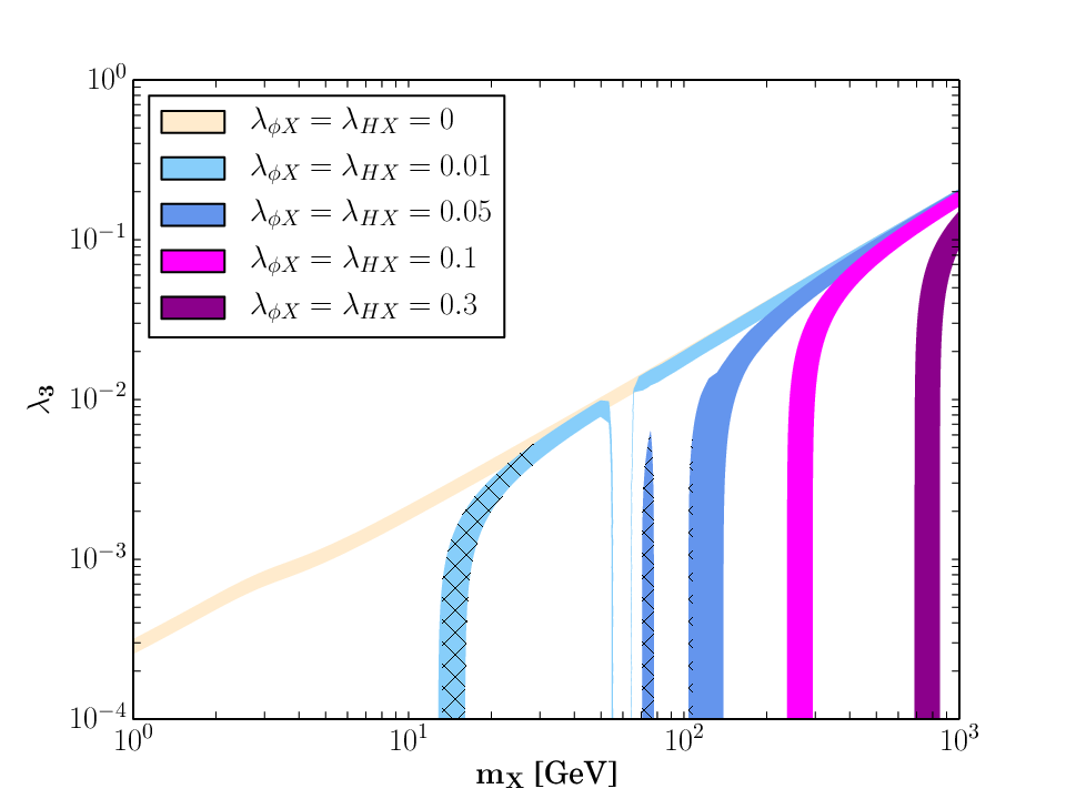
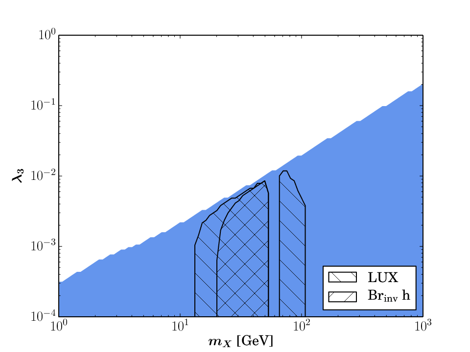
As we did for the self-annihilation case, in Fig. 11 we show the region of the parameter space that could give rise to the measures DM relic abundance in the plane $[m_{X},\,\lambda_{3}]$ after marginalizing with respect to $\lambda_{HX}$ and $\lambda_{\phi X}$. The white region, corresponding to large values for $\lambda_{3}$, always generates a DM underabundance. Moreover, assuming that the cross-section for the semi-annihilation into a GB is never greater than about $\langle\sigma v\rangle_{\text{semi}}\sim 3\cdot 10^{-26}$ cm³/s, this translates into the upper bound

which can be seen in Fig. 11. In addition, we also show both the LUX and the Higgs invisible decay exclusion limits.

In spite of the great success of the $\Lambda$CDM scenario in explaining the formation and evolution of cosmic structures, there are some problems at small scales (see, e.g. [50]). Simulations of this scenario result in cuspy density profile of halos towards its center and a large number of small satellite halos. These results are challenged by observations. Although the inclusion of baryonic effects can ameliorate the discrepancies, it is still unclear whether it is necessary to change the physics of the DM sector. For instance, self-interacting DM with a strength [51, 52, 53, 54, 55, 56, 57, 58]:

can help in solving the observed discrepancies. Yet, the Bullet Cluster [59, 60, 61] and recent analysis of the constraints from halo shapes [54, 56, 55], favor the following upper bound on the DM self-interacting cross section (at velocities greater than 300 km/s)

The corresponding elastic scattering processes in our model are shown in Fig. 12.

From the diagrams it is possible to see that the exchange of a $\rho$ or a $h$ boson lighter than the DM can possibly lead to non-perturbative effects such as long range interactions. In this section we limit ourselves to the perturbative scenario and we therefore assume $m_{\rho}$, $m_{h}\gg m_{X}$. A posteriori we will find that this is also necessary for the DM production to take place via the $3\to 2$ annihilation process (see section 5.2). Under this assumption the elastic scattering cross-section in the non-relativistic limit reads

where ${\cal Z}\equiv\lambda_{3}\,v_{\phi}/m_{X}$. The ${\cal Z}$ parameter can not be arbitrarily large. In fact, perturbative unitarity requires the $s$-wave amplitude of the process $X\bar{X}\to X\bar{X}$ to be bounded from above [62]. Considering $m_{\rho}$ and $m_{h}\gg m_{X}$, this translate into

which implies the following weaker bounds

The process $XX\to XX$ also sets an upper bound on the same parameters, however it is never as stringent as the one of Eq. (27).

Fig. 13 shows the regions of the plane $[\lambda_{X},\,{\cal Z}]$ fulfilling Eq. (24) for different values of the DM mass. In addition, we depict the areas disfavored by the Bullet Cluster for those masses (i.e. Eq. (25)) and we also hatch the regions where perturbative unitarity is lost.

In this figure a limit on the DM mass is manifest, corresponding to

which is the mass that saturates the perturbative unitary bound of (28) and that is still in agreement with the astrophysical lower bound of Eq. (24).

Instead of the usual $2\to 2$ annihilation scenarios described in previous sections, another mechanism for the reduction of the comoving DM number density is the annihilation via $3\to 2$ processes. Here we discuss this case, assuming that it is the dominant process for the relic density computation, or equivalently that $\gamma_{\text{self}}$, $\gamma_{\text{semi}}\ll\gamma_{3\to 2}$ at the epoch of the freeze-out.

As explained in the Appendix A, it is necessary for the DM to release the kinetic energy produced in the $3\to 2$ reactions. This can be fulfilled if DM is in kinetic equilibrium with either SM particles or the GBs. The first possibility is realized by means of DM scattering off electrons. However, it requires a large Higgs portal. This can be understood from the effective Lagrangian between electrons and DM. Assuming $m_{h},\,m_{\rho}\gg m_{X}$ and $\theta\ll 1$, we have

and one can write

where $m_{e}$ is the electron mass. In order to keep the kinetic equilibrium between the DM and the electrons from this interaction, it is necessary that $\epsilon\gtrsim 5\times 10^{-9}$ [25], or equivalently, that $\lambda_{HX}\gtrsim 1.5\times 10^{3}\,(m_{e}/m_{X})$, which is too large if Eq. (29) holds.

As a result, the only possibility is to have kinetic equilibrium between the DM with the GBs. The corresponding rate depends on $\lambda_{\phi X}$ and for $m_{h},\,m_{\rho}\gg m_{X}$ is mostly driven by a contact interaction (see Fig 6). Because of this, it is not suppressed by a heavy scale in contrast to the previous case. Moreover, although this scattering rate should be greater than the Hubble parameter at the epoch of the freeze-out, we must insure that the rate for the self-annihilation process into GBs -which is obtained by crossing symmetry- is negligible. This is possible because $\Gamma_{\text{kin}}/\Gamma_{\text{ann}}\sim n_{\eta}/n_{\text{DM}}\gg 1$ at the freeze-out, due to the sub-dominance of $n_{\text{DM}}$ during the radiation-dominated epoch. We conclude that $\lambda_{\phi X}$ must be sizable but not too large in order to avoid self-annihilations into GBs.

In section 3.1, it was implicitly assumed that the GB did not heat up after its decoupling from the SM plasma. In fact, this is not the case here because DM is not in kinetic equilibrium with the SM and transfers all its entropy exclusively to the GBs when it annihilates via the $3\to 2$ mechanism. As a result, Eq. (13) must be modified accordingly in order to account for this effect and thus $T^{d}_{\eta}$ must be larger than the muon mass so that the contribution to $N_{\text{eff}}$ is negligeable. This always takes place here because we consider $m_{h},\,m_{\rho}\gg m_{X}\sim 100$ MeV, which implies that the processes establishing the equilibrium are very suppressed for temperatures around the muon mass.

With this in mind, we can consider the $3\to 2$ reactions in this model. All of them are equivalent, up to $CP$ conjugation, to either $\bar{X}\,\bar{X}\,X\to X\,X$ or $X\,X\,X\to X\,\bar{X}$. In Figs. 14 and 15 we show the corresponding diagrams at tree-level. The corresponding cross-sections can be calculated analytically if we work in the non-relativistic approximation (see Appendix B). In fact, the resulting expressions can be further simplified in the case $\gamma_{\text{self}}\ll\gamma_{3\to 2}$ because of the following reason. As for self-annihilation, some of the $3\to 2$ diagrams are proportional to $\lambda_{HX}$ and $\lambda_{\phi X}$. In fact, this happens for those in the first and second rows of Figs. 14 and 15 simply because they involve exchange of $\rho$ or $h$ particles. In contrast, the diagrams of the third and fourth lines depend uniquely on different couplings, namely $\lambda_{3}$ and $\lambda_{X}$. Consequently, the contribution of the first set of diagrams is presumably negligible, if self-annihilations are subdominant. The fact that $m_{\rho}$ and $m_{h}\gg m_{X}$ reinforces this argument. However, notice that for this to be true it is not necessary that $\lambda_{\phi X}$ vanishes. Under these assumptions we find

where ${\cal Z}=\lambda_{3}\,v_{\phi}/m_{X}$ was already introduced. Because self- and semi-annihilations into GBs are always kinematically allowed, Eq. (32) must be compared with the cross-sections associated to these processes

We already discussed the first process. Regarding the second one, although $\langle\sigma v\rangle_{\text{semi}}$ and $\langle\sigma v^{2}\rangle_{3\to 2}$ have different mass dimensions and can not be compared directly, it is clear that the semi-annihilations are suppressed for small $\lambda_{3}$, and that the $3\to 2$ is important when ${\cal Z}$ is large. Moreover, a suppression in the $3\to 2$ process due to $\lambda_{3}$ can be compensated with a large $v_{\phi}$ with respect to the DM mass. Under these circumstances we can make sure that $\gamma_{\text{self}}$, $\gamma_{\text{semi}}\ll\gamma_{3\to 2}$, while still having kinetic equilibrium between the GBs and the DM. We remark that the DM mass is not required to be in the GeV range because we assume no equilibrium between the GBs and SM plasma and consequently there is no significant contribution to $N_{\text{eff}}$.

In order to study the regions of the parameter space where the $3\to 2$ reproduces the observed relic abundance, instead of solving numerically the Boltzmann equations directly we work in the freeze-out approximation.

When the temperature of the plasma is much greater than the DM mass, the Boltzmann Eq. (9) has the solution $n=n_{\text{eq}}$, which corresponds to the chemical equilibrium. However, once the temperature drops below the DM mass, the rate for the process $2\to 3$ is kinematically suppressed compared to the $3\to 2$ reaction. As a result the DM number density deviates from its equilibrium value. In fact, it eventually becomes much greater than its equilibrium value $n\gg n_{\text{eq}}$. Hence, for these temperatures and when there are no self- and semi-annihilations, Eq. (9) can be approximated by

When the DM particles are non-relativistic, the cross-section $\langle\sigma v^{2}\rangle$ is independent of the temperature. In that case, using standard methods, Eq. (34) admits the following solution

where FO stands for the freeze-out, $g$ are the number of relativistic degrees of freedom and $x=m_{X}/T$. Here $T$ is the DM temperature which equals that of the GB plasma. It is remarkable that, in contrast to the standard self-annihilation scenario, here the cross-section that matches the observed relic density depends on the DM mass. In order to estimate $x_{\text{FO}}$, it is necessary to establish when the annihilation rate per particle $n_{\text{eq}}^{2}\langle\sigma v\rangle_{3\to 2}$ drops below the expansion rate of the Universe. Using Eq. (35) it is found that this happens when freeze-out temperature satisfies

Because the second term of this equation depends logarithmically on the DM mass, it is a very good approximation to take $x_{\text{FO}}\approx 20$.

It is somewhat interesting to calculate the value of $\langle\sigma v\rangle_{2\to 3}$ associated to Eq. (35). To that end, notice that at the freeze-out the expansion rate is $H=n_{\text{eq}}\,\langle\sigma v\rangle_{2\to 3}=n_{\text{eq}}^{2}\langle\sigma v^{2}\rangle_{3\to 2}$ and as a result $n_{\text{eq}}=\sqrt{H/\langle\sigma v^{2}\rangle_{3\to 2}}$. According to Eq. (49) we obtain

In contrast to Eq. (35), notice that this equation is independent of the DM mass and is similar to the usual condition for the WIMP scenario.

We use this formalism in order to calculate the relic density. In Fig. 16 we show the regions of the plane $[\lambda_{X},\,{\cal Z}]$ in agreement with the observed relic density for different values of the DM mass when the $3\to 2$ process dominates the DM production. They are obtained using Eqs. (32) and (35), taking into account an uncertainty of $25\%$ in order to account for the error in the freeze-out and the non-relativistic approximations. As apparent from the figure, there are two regimes. On the one hand, for small values of $\lambda_{X}$ the DM abundance is set by ${\cal Z}$. On the other hand, when $\lambda_{X}$ is of order one both variables are relevant for the DM dynamics. In particular notice that ${\cal Z}$ can not vanish. Fig. 16 also includes the region where perturbative unitarity is lost, which implies an upper limit on the DM mass as shown in the figure:

Let us note that this limit, obtained from the relic density, is comparable to the one in Eq. (29) coming from demanding significant DM self-interactions.

It is interesting that the variables that control DM self-interactions also determine the $3\to 2$ process, as shown in Eqs. (26) and (32). This suggests that both phenomena have a common origin, which we attribute to the fact that DM is strongly interacting. Fig. 17 illustrates this by showing the regions of the parameter space where the relic abundance is generated via the $3\to 2$ mechanism and where the self-interaction cross-section simultaneously fulfills the astrophysical hints from small scale structures, as in Eq. (24). In addition, we show the areas disfavored by the Bullet Cluster (i.e. Eq. (25)). All this has been done under the assumption that perturbative unitarity is valid.

The figure conclusively shows that the DM mass is bounded both from above and below

which is in agreement with the findings of [25]. Similarly, for the ${\cal Z}$ parameter we find

We illustrate this scenario with three benchmark points which are defined in Table 1 and shown in Fig. 17. They correspond to different masses in the MeV range, which reproduce simultaneously the observed relic abundance via the $3\to 2$ mechanism and the hints on the self-interaction cross-section. Whereas points B and C give rise to a $\sigma_{\text{scatter}}/m_{X}$ in agreement with the Bullet Cluster observations, point A is disfavored due to its small mass. In every case $\lambda_{3}$, $\lambda_{HX}$ and $\lambda_{\phi X}$ are chosen small enough in order to ensure that semi-annihilations and self-annihilations are subdominant (see Table 1). Nevertheless, we require that DM is in kinetic equilibrium with the GBs via the $\lambda_{\phi X}$ coupling, as argued before. We again find that the scale at which the $U(1)_{\text{DM}}$ symmetry breaks down has to be at least in the TeV range so that ${\cal Z}$ is of order one. We would like to remark that all these points are in agreement with collider constraints because the $\rho$ boson is very heavy and the invisible decay width of the Higgs is very small. In fact, the most important contribution to the latter comes from the process $h\to X\bar{X}$ with a branching ratio of approximately $1.5\cdot 10^{-5}$. The other channels ($\rho\rho$, $\eta\eta$, $XXX$ and $\bar{X}\bar{X}\bar{X}$) contribute less than $\sim 10^{-12}$.

References

- (1) G. Jungman, M. Kamionkowski, and K. Griest, Supersymmetric dark matter, Phys.Rept. 267 (1996) 195–373, [hep-ph/9506380].
- (2) L. Bergström, Nonbaryonic dark matter: Observational evidence and detection methods, Rept.Prog.Phys. 63 (2000) 793, [hep-ph/0002126].
- (3) C. Muñoz, Dark matter detection in the light of recent experimental results, Int.J.Mod.Phys. A19 (2004) 3093–3170, [hep-ph/0309346].
- (4) G. Bertone, D. Hooper, and J. Silk, Particle dark matter: Evidence, candidates and constraints, Phys.Rept. 405 (2005) 279–390, [hep-ph/0404175].
- (5) L. Bergström, Dark matter evidence, particle physics candidates and detection methods, Annalen der Physik 524 (2012) 479–496, [arXiv:1205.4882].
- (6) G. F. Giudice, Naturalness after LHC8, PoS EPS-HEP2013 (2013) 163, [arXiv:1307.7879].
- (7) M. Bento, O. Bertolami, R. Rosenfeld, and L. Teodoro, Selfinteracting dark matter and invisibly decaying Higgs, Phys.Rev. D62 (2000) 041302, [astro-ph/0003350].
- (8) M. Bento, O. Bertolami, and R. Rosenfeld, Cosmological constraints on an invisibly decaying Higgs boson, Phys.Lett. B518 (2001) 276–281, [hep-ph/0103340].
- (9) M. Gonderinger, Y. Li, H. Patel, and M. J. Ramsey-Musolf, Vacuum Stability, Perturbativity, and Scalar Singlet Dark Matter, JHEP 1001 (2010) 053, [arXiv:0910.3167].
- (10) V. Silveira and A. Zee, Scalar phantoms, Phys.Lett. B161 (1985) 136.
- (11) J. McDonald, Gauge singlet scalars as cold dark matter, Phys.Rev. D50 (1994) 3637–3649, [hep-ph/0702143].
- (12) C. Burgess, M. Pospelov, and T. ter Veldhuis, The Minimal model of nonbaryonic dark matter: A Singlet scalar, Nucl.Phys. B619 (2001) 709–728, [hep-ph/0011335].
- (13) J. M. Cline, K. Kainulainen, P. Scott, and C. Weniger, Update on scalar singlet dark matter, Phys.Rev. D88 (2013) 055025, [arXiv:1306.4710].
- (14) L. Feng, S. Profumo, and L. Ubaldi, Closing in on singlet scalar dark matter: LUX, invisible Higgs decays and gamma-ray lines, JHEP 1503 (2015) 045, [arXiv:1412.1105].
- (15) T. Hambye, Hidden vector dark matter, JHEP 0901 (2009) 028, [arXiv:0811.0172].
- (16) F. D’Eramo and J. Thaler, Semi-annihilation of Dark Matter, JHEP 1006 (2010) 109, [arXiv:1003.5912].
- (17) G. Bélanger, K. Kannike, A. Pukhov, and M. Raidal, Impact of semi-annihilations on dark matter phenomenology - an example of symmetric scalar dark matter, JCAP 1204 (2012) 010, [arXiv:1202.2962].
- (18) G. Bélanger, K. Kannike, A. Pukhov, and M. Raidal, Minimal semi-annihilating scalar dark matter, JCAP 1406 (2014) 021, [arXiv:1403.4960].
- (19) B. Moore, Evidence against dissipationless dark matter from observations of galaxy haloes, Nature 370 (1994) 629.
- (20) R. A. Flores and J. R. Primack, Observational and theoretical constraints on singular dark matter halos, Astrophys.J. 427 (1994) L1–4, [astro-ph/9402004].
- (21) S.-H. Oh, C. Brook, F. Governato, E. Brinks, L. Mayer, et al., The central slope of dark matter cores in dwarf galaxies: Simulations vs. THINGS, Astron.J. 142 (2011) 24, [arXiv:1011.2777].
- (22) M. G. Walker and J. Peñarrubia, A Method for Measuring (Slopes of) the Mass Profiles of Dwarf Spheroidal Galaxies, Astrophys.J. 742 (2011) 20, [arXiv:1108.2404].
- (23) M. Boylan-Kolchin, J. S. Bullock, and M. Kaplinghat, Too big to fail? The puzzling darkness of massive Milky Way subhaloes, Mon.Not.Roy.Astron.Soc. 415 (2011) L40, [arXiv:1103.0007].
- (24) S. Garrison-Kimmel, M. Boylan-Kolchin, J. S. Bullock, and E. N. Kirby, Too Big to Fail in the Local Group, Mon.Not.Roy.Astron.Soc. 444 (2014) 222, [arXiv:1404.5313].
- (25) Y. Hochberg, E. Kuflik, T. Volansky, and J. G. Wacker, Mechanism for Thermal Relic Dark Matter of Strongly Interacting Massive Particles, Phys.Rev.Lett. 113 (2014) 171301, [arXiv:1402.5143].
- (26) Y. Hochberg, E. Kuflik, H. Murayama, T. Volansky, and J. G. Wacker, The SIMPlest Miracle, arXiv:1411.3727.
- (27) G. Bélanger, K. Kannike, A. Pukhov, and M. Raidal, Scalar Singlet Dark Matter, JCAP 1301 (2013) 022, [arXiv:1211.1014].
- (28) P. Ko and Y. Tang, Self-interacting scalar dark matter with local symmetry, JCAP 1405 (2014) 047, [arXiv:1402.6449].
- (29) L. M. Krauss and F. Wilczek, Discrete Gauge Symmetry in Continuum Theories, Phys.Rev.Lett. 62 (1989) 1221.
- (30) D. Aristizábal Sierra, M. Dhen, C. S. Fong, and A. Vicente, Dynamical flavor origin of symmetries, arXiv:1412.5600.
- (31) A. Djouadi, The Anatomy of electro-weak symmetry breaking. I: The Higgs boson in the standard model, Phys.Rept. 457 (2008) 1–216, [hep-ph/0503172].
- (32) N. D. Christensen and C. Duhr, FeynRules - Feynman rules made easy, Comput.Phys.Commun. 180 (2009) 1614–1641, [arXiv:0806.4194].
- (33) N. D. Christensen, P. de Aquino, C. Degrande, C. Duhr, B. Fuks, et al., A Comprehensive approach to new physics simulations, Eur.Phys.J. C71 (2011) 1541, [arXiv:0906.2474].
- (34) A. Belyaev, N. D. Christensen, and A. Pukhov, CalcHEP 3.4 for collider physics within and beyond the Standard Model, Comput.Phys.Commun. 184 (2013) 1729–1769, [arXiv:1207.6082].
- (35) G. Bélanger, F. Boudjema, A. Pukhov, and A. Semenov, MicrOMEGAs 2.0: A Program to calculate the relic density of dark matter in a generic model, Comput.Phys.Commun. 176 (2007) 367–382, [hep-ph/0607059].
- (36) G. Bélanger, F. Boudjema, A. Pukhov, and A. Semenov, micrOMEGAs_3: A program for calculating dark matter observables, Comput.Phys.Commun. 185 (2014) 960–985, [arXiv:1305.0237].
- (37) B. W. Lee and S. Weinberg, Cosmological Lower Bound on Heavy Neutrino Masses, Phys.Rev.Lett. 39 (1977) 165–168.
- (38) T. Hambye and M. H. Tytgat, Confined hidden vector dark matter, Phys.Lett. B683 (2010) 39–41, [arXiv:0907.1007].
- (39) P. Gondolo and G. Gelmini, Cosmic abundances of stable particles: Improved analysis, Nucl.Phys. B360 (1991) 145–179.
- (40) Planck Collaboration, P. Ade et al., Planck 2013 results. XVI. Cosmological parameters, Astron.Astrophys. (2014) [arXiv:1303.5076].
- (41) G. Steigman, Equivalent Neutrinos, Light WIMPs, and the Chimera of Dark Radiation, Phys.Rev. D87 (2013), no. 10 103517, [arXiv:1303.0049].
- (42) Planck Collaboration, P. Ade et al., Planck 2015 results. XIII. Cosmological parameters, arXiv:1502.0158.
- (43) G. Steigman, private communication.
- (44) S. Weinberg, Goldstone Bosons as Fractional Cosmic Neutrinos, Phys.Rev.Lett. 110 (2013), no. 24 241301, [arXiv:1305.1971].
- (45) C. Garcia-Cely, A. Ibarra, and E. Molinaro, Dark matter production from Goldstone boson interactions and implications for direct searches and dark radiation, JCAP 1311 (2013) 061, [arXiv:1310.6256].
- (46) P. Bechtle, S. Heinemeyer, O. Stål, T. Stefaniak, and G. Weiglein, Probing the Standard Model with Higgs signal rates from the Tevatron, the LHC and a future ILC, JHEP 1411 (2014) 039, [arXiv:1403.1582].
- (47) CMS Collaboration, V. Khachatryan et al., Constraints on the Higgs boson width from off-shell production and decay to Z-boson pairs, Phys.Lett. B736 (2014) 64, [arXiv:1405.3455].
- (48) OPAL Collaboration, G. Abbiendi et al., Decay mode independent searches for new scalar bosons with the OPAL detector at LEP, Eur.Phys.J. C27 (2003) 311–329, [hep-ex/0206022].
- (49) LUX Collaboration, D. Akerib et al., First results from the LUX dark matter experiment at the Sanford Underground Research Facility, Phys.Rev.Lett. 112 (2014) 091303, [arXiv:1310.8214].
- (50) D. H. Weinberg, J. S. Bullock, F. Governato, R. K. de Naray, and A. H. G. Peter, Cold dark matter: controversies on small scales, arXiv:1306.0913.
- (51) D. N. Spergel and P. J. Steinhardt, Observational evidence for self-interacting cold dark matter, Phys.Rev.Lett. 84 (2000) 3760–3763, [astro-ph/9909386].
- (52) B. D. Wandelt, R. Dave, G. R. Farrar, P. C. McGuire, D. N. Spergel, et al., Self-interacting dark matter, astro-ph/0006344.
- (53) M. Vogelsberger, J. Zavala, and A. Loeb, Subhaloes in Self-Interacting Galactic Dark Matter Haloes, Mon.Not.Roy.Astron.Soc. 423 (2012) 3740, [arXiv:1201.5892].
- (54) M. Rocha, A. H. Peter, J. S. Bullock, M. Kaplinghat, S. Garrison-Kimmel, et al., Cosmological Simulations with Self-Interacting Dark Matter I: Constant Density Cores and Substructure, Mon.Not.Roy.Astron.Soc. 430 (2013) 81–104, [arXiv:1208.3025].
- (55) A. H. Peter, M. Rocha, J. S. Bullock, and M. Kaplinghat, Cosmological Simulations with Self-Interacting Dark Matter II: Halo Shapes vs. Observations, Mon.Not.Roy.Astron.Soc. 430 (2012) 105–120, [arXiv:1208.3026].
- (56) J. Zavala, M. Vogelsberger, and M. G. Walker, Constraining Self-Interacting Dark Matter with the Milky Way’s dwarf spheroidals, Mon.Not.Roy.Astron.Soc.: Letters 431 (2013) L20–L24, [arXiv:1211.6426].
- (57) M. Vogelsberger, J. Zavala, C. Simpson, and A. Jenkins, Dwarf galaxies in CDM and SIDM with baryons: observational probes of the nature of dark matter, Mon.Not.Roy.Astron.Soc. 444 (2014) 3684, [arXiv:1405.5216].
- (58) O. D. Elbert, J. S. Bullock, S. Garrison-Kimmel, M. Rocha, J. Oñorbe, et al., Core Formation in Dwarf Halos with Self Interacting Dark Matter: No Fine-Tuning Necessary, arXiv:1412.1477.
- (59) D. Clowe, A. Gonzalez, and M. Markevitch, Weak lensing mass reconstruction of the interacting cluster 1E0657-558: Direct evidence for the existence of dark matter, Astrophys.J. 604 (2004) 596–603, [astro-ph/0312273].
- (60) M. Markevitch, A. Gonzalez, D. Clowe, A. Vikhlinin, L. David, et al., Direct constraints on the dark matter self-interaction cross-section from the merging galaxy cluster 1E0657-56, Astrophys.J. 606 (2004) 819–824, [astro-ph/0309303].
- (61) S. W. Randall, M. Markevitch, D. Clowe, A. H. Gonzalez, and M. Bradač, Constraints on the Self-Interaction Cross-Section of Dark Matter from Numerical Simulations of the Merging Galaxy Cluster 1E 0657-56, Astrophys.J. 679 (2008) 1173–1180, [arXiv:0704.0261].
- (62) W. Kilian, Dynamical electroweak symmetry breaking, hep-ph/0303015.
- (63) J. Bernstein, L. S. Brown, and G. Feinberg, The Cosmological Heavy Neutrino Problem Revisited, Phys.Rev. D32 (1985) 3261.
- (64) E. D. Carlson, M. E. Machacek, and L. J. Hall, Self-interacting dark matter, Astrophys.J. 398 (1992) 43–52.
- (65) M. Machacek, Growth of adiabatic perturbations in selfinteracting dark matter, Astrophys.J. 431 (1994) 41–51.
- (66) A. A. de Laix, R. J. Scherrer, and R. K. Schaefer, Constraints of selfinteracting dark matter, Astrophys.J. 452 (1995) 495, [astro-ph/9502087].
- (67) N. Yamanaka, S. Fujibayashi, S. Gongyo, and H. Iida, Dark matter in the hidden gauge theory, arXiv:1411.2172.